The OH line contamination of 21 cm intensity fluctuation measurements for $z=1\sim 4$

Abstract

The large-scale structure of the Universe can be mapped with unresolved intensity fluctuations of the 21 cm line. The power spectrum of the intensity fluctuations has been proposed as a probe of the baryon acoustic oscillations at low to moderate redshifts with interferometric experiments now under consideration. We discuss the contamination to the low-redshift 21 cm intensity power spectrum generated by the 18 cm OH line since the intensity fluctuations of the OH line generated at a slightly higher redshift contribute to the intensity fluctuations observed in an experiment. We assume the OH megamaser luminosity is correlated with the star formation rate, and use the simulation to estimate the OH signal and the spatial anisotropies. We also use a semi-analytic simulation to predict the 21 cm power spectrum. At $z=1$ to 3, we find that the OH contamination could reach 0.1 to 1% of the 21 cm rms fluctuations at the scale of the first peak of the baryon acoustic oscillation. When $z>3$ the OH signal declines quickly, so that the contamination on the 21-cm becomes negligible at high redshifts.

1. Introduction

The large-scale structure of the Universe can be observed efficiently with the intensity mapping technique, where the distribution of the radiation intensity of a particular line emission from large volume cells is observed without attempting to resolve the individual emitters, galaxies, within the volume. This technique is particularly suitable for radio observations, where the angular resolution is relatively low. By observing the radiation at different wavelengths, the emissivity from different redshifts are obtained, thus revealing the three dimensional matter distribution on large scales. It was first recognized that this method can be applied to the 21cm line of the neutral hydrogen (Chang et al., 2008; Peterson et al., 2009; Chang et al., 2010), and provides a very powerful tool for precise determination of the equation of state of dark energy by using the baryon acoustic oscillation (BAO) peak of large-scale structure as a standard ruler (Chang et al., 2008; Ansari et al., 2008; Seo et al., 2010). More recently, it has also been proposed that the intensity mapping method be used for molecular and fine-structure lines, such as CO (Gong et al., 2011; Carilli, 2011; Lidz et al., 2011; Visbal & Loeb, 2010) and CII (Gong et al., 2011b).

A possible problem with the intensity mapping technique is the contamination by other lines. Unlike the observation of individual sources, where different lines from two different sources overlapping along the line of sight can be separated through high-resolution imaging, in intensity mapping the contamination from a different line at a different redshift cannot be easily separated. For optical (e.g. the Lyman $\alpha$ line) and for many of the important radio lines, there are many spectral lines with wavelengths longer than the line being observed, thus emitters at lower redshifts could become contaminants and these could be obstacles in the application of this method. An advantage of the 21cm line for intensity mapping is that due to its low frequency (1420 MHz), there are few strong lines at a lower redshift which could contaminate the observations.

Nevertheless, the hydroxyl radical (OH) lines of 18 cm wavelength at slightly higher redshifts can potentially contaminate HI 21 cm observations at lower redshifts . The $\lambda=$ 18 cm lines of OH correspond to four possible transitions, with frequencies at 1612, 1665, 1667, and 1720 MHz. Strong OH emission are produced by masers, originating typically in high density ($n(H_{2})>10^{7}{\rm cm}^{-3})$ gas near an excitation source, though the exact environment for the masers to happen is still not clear (Lo, 2005). The 1665MHz and 1667MHz are usually much stronger than the other two lines, hence are named “main lines”. In masers, the 1667MHz line is the strongest, whose flux is typically about 2 to 20 times greater than the 1665MHz line (Randell et al., 1995).

In an intensity mapping observation, the 21 cm auto-correlation power spectrum at a redshift $z$ is observed. However, the OH emission at $1+z^{\prime}=(1+z)\frac{\lambda_{\rm HI}}{\lambda_{\rm OH}}$ would also give raise to brightness temperature fluctuations which can not be distinguished from the redshifted 21cm fluctuations in such observations. Thus, for example, the HI 21-cm signal at $z_{\rm HI}=1,2$ and 3 would be contaminated by the OH 18cm emission at $z_{\rm OH}=1.35,2.52,$ and 3.70 respectively. Since the OH fluctuations at redshift $z^{\prime}$ are uncorrelated with the 21 cm fluctuations at redshift $z$, the two power spectra would simply add. Although the OH line emission is produced with a different mechanism and depends on the star formation activity, on large scales, we still expect the OH intensity fluctuations to trace the total matter densities. Its power spectrum should be proportional to the matter power spectrum at $z^{\prime}$, with a different bias factor. If not properly accounted for, this may introduce a distortion to the total intensity power spectrum extracted from the 21 cm observations resulting in a shift to the BAO peaks. Given the low-redshift 21 cm BAO experiments are now being developed (e.g. the proposal to conduct wider area surveys with GBT by building a multi-beam receiver, the Tianlai project in China, and the CHIME project in Canada) it is important to estimate the magnitude of the potential contamination.

For this purpose, we make use of simulations to predict both the 21 cm and OH intensity power spectrum from $z=1$ to 4. We find that the contamination is generally small and below 1% of the rms fluctuations at $z=1$ to 3 with a large uncertainty related to the overall predictions on the OH signal. The paper is organized as follows: In the next section we present the method of the intensity calculation and in Section 3 we present our results and discuss the contamination. We will assume WMAP 7-year flat $\Lambda$CDM cosmological model (Komatsu et al., 2011).

2. Calculation

In order to estimate the 21 cm emission at low redshifts, we make use of the semi-analytic simulations by Obreschkow et al. (2009), which are available as part of the SKA Simulated Skies , and based on the galaxy catalog derived from the Millennium simulation (De Lucia et al., 2007; Springel et al., 2005). These are the same simulations we have used in Gong et al. (2011). As the HI mass of each galaxy is assigned using the galaxy properties provided by the semi-analytical modeling of galaxy formation, we will use those neutral hydrogen masses to calculate the 21 cm line intensities.

The calculation of the 21 cm power spectrum is similar to what we have done in Gong et al. (2011). The 21 cm temperature from galaxies, assuming the signal is seen in emission is (Santos et al., 2008)

$$\bar{T}^{\rm G}_{\rm b}=c(z)\frac{\rho_{\rm HI}}{X_{\rm H}\rho_{\rm b}}\,(\rm mK),$$ (1)

where $X_{\rm H}=0.74$ is the mean hydrogen mass fraction in the Universe, $\rho_{\rm b}=\Omega_{\rm b}\rho_{\rm c}$ is the baryon density and $\rho_{\rm c}$ is the critical density. The $c(z)$ takes the form as

$$c(z)\approx 23\bigg{(}\frac{0.7}{h}\bigg{)}\bigg{(}\frac{\Omega_{\rm b}h^{2}}{0.02}\bigg{)}\bigg{(}\frac{0.15}{\Omega_{\rm m}h^{2}}\frac{1+z}{10}\bigg{)}^{1/2}({\rm mK}).$$ (2)

The parameter $c(z)\bar{x}_{\rm H}$ gives the mean brightness temperature of the 21-cm emission, where $\bar{x}_{\rm H}$ is the mean neutral fraction. We assume that the neutral hydrogen are mostly contained within the galaxies after reionization, the mass density $\rho_{\rm HI}$ is then given by

$$\rho_{\rm HI}=\int_{M_{\rm min}}^{M_{\rm max}}dM\frac{dn}{dM}M_{\rm HI}(M),$$ (3)

where $dn/dM$ is the mass function, we take $M_{\rm min}=10^{8}\ \rm M_{\odot}/h$ to be the minimum mass for a halo to retain neutral hydrogen (Loeb & Barkana, 2001), and $M_{\rm max}=10^{13}\ \rm M_{\odot}/h$ is the maximum mass for which the gas have sufficient time to cool and form galaxies (the result is insensitive to this number).

In above the $M_{\rm HI}$ is the neutral hydrogen mass in a halo with mass $M$. The HI mass is correlated with the halo mass, though with some scatter. Inspired by the shape of the distribution seen in the semi-analytic simulation generated from Obreschkow et al. (2009), we fit a relation of the form

$$M_{\rm HI}(M)=A\times\left(1+\frac{M}{c_{1}}\right)^{b}\left(1+\frac{M}{c_{2}}\right)^{d}\,.$$ (4)

The best-fit values of the parameters $A$, $c_{1}$, $c_{2}$, $b$ and $d$ are given in Table 1.

Due to the mass resolution limit of the Millennium simulation, for $M<10^{10}\ M_{\odot}$, we cannot use the same fitting formula. Instead we assume $M_{\rm HI}=X_{\rm HI}^{\rm gal}(\Omega_{b}/\Omega_{m})M$ to estimate the neutral hydrogen mass in halos, where $X_{\rm HI}^{\rm gal}$ is the neutral hydrogen mass fraction in the galaxy. We set $X_{\rm HI}^{\rm gal}=0.15$ which is estimated at $M=10^{10}\ M_{\odot}$ in the simulation, and assume it does not change when $M<10^{10}\ M_{\odot}$. The simulation result and the best fitting curves at $z=1$, $z=2$ and $z=3$ are shown in the upper panel of Fig. 1, which are consistent with the other results (e.g. Marin et al. (2010); Duffy et al. (2011)).

We find the HI energy density parameter $\Omega_{\rm HI}=\rho_{\rm HI}/\rho_{c}$ is about $10^{-3}$ and insensitive to the redshift (for $z\lesssim 3$) in our calculation, which is consistent with the observational results (e.g. Rao et al. (2006); Lah et al. (2007); Noterdaeme et al. (2009)). Finally, we find the 21-cm mean brightness temperature are 481, 573 and 544 $\mu$K at z=1, 2 and 3 respectively. These values are also consistent with an observation at $z=0.94$ (Chang et al., 2010) and previous predictions in the literature (Chang et al., 2008).

Assuming that the 21 cm flux from galaxies is proportional to the neutral hydrogen mass $M_{\rm HI}$, then the 21 cm signal will follow the underlying dark matter distribution with a bias

$$b_{\rm HI}(z)=\frac{\int_{M_{\rm min}}^{M_{\rm max}}dM\frac{dn}{dM}M_{\rm HI}b(z,M)}{\rho_{\rm HI}}.$$ (5)

where $b(z,M)$ is the halo bias (Sheth & Tormen, 1999). The 21-cm temperature from galaxies is then $T^{\rm G}_{\rm b}({\bf x})=\bar{T}^{\rm G}_{\rm b}[1+b_{\rm HI}\delta({\bf x})]$, and the clustering power spectrum is given by $P^{\rm G}_{\rm HI}(z,k)=\left(\bar{T}^{\rm G}_{\rm b}\right)^{2}b^{2}_{\rm HI}P(k,z).$ We use the $\tt Halofit$ code (Smith et al., 2003) to calculate the non-linear matter power spectrum $P(k,z)$. Additionally, there is a shot noise contribution to the power spectrum due to the discreteness of galaxies,

$$P^{\rm shot}_{\rm HI}(z)=\int_{M_{\rm min}}^{M_{\rm max}}dM\frac{dn}{dM}\left[c(z)\frac{M_{\rm HI}}{X_{\rm H}\rho_{\rm b}}\right]^{2}.$$ (6)

Table 1The best-fit values of the parameters in the $M_{\rm HI}$-$M$ relation.

	$z=1$	$z=2$	$z=3$
$A$	$2.1\times 10^{8}$	$2.1\times 10^{8}$	$1.7\times 10^{8}$
$c_{1}$	$1.0\times 10^{11}$	$1.0\times 10^{11}$	$1.0\times 10^{11}$
$c_{2}$	$4.55\times 10^{11}$	$5.60\times 10^{11}$	$5.0\times 10^{11}$
$b$	$2.65$	$2.4$	$2.4$
$d$	$-2.64$	$-2.40$	$-2.25$

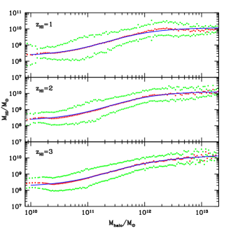
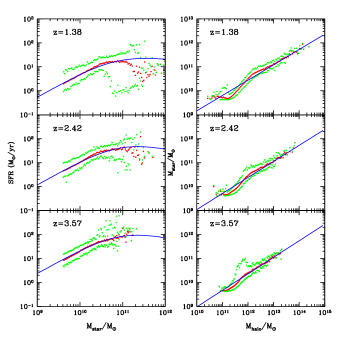
Figure 1.— Upper panel: the $M_{\rm HI}$-$M$ relation from the simulation at $z=1$, $z=2$ and $z=3$. Lower panel: the SFR vs. the stellar mass $M_{\star}$ and the stellar mass vs. the halo mass at different redshifts as derived from the galaxy catalog in De Lucia et al. (2007). The red dots are the mean value and the green dots show the 1$\sigma$ error from the simulation. The best fits are shown in blue solid line.

While the OH molecule is not as abundant as neutral hydrogen, the OH maser is brighter than the 21 cm line intensity for the same number density of baryons. It is believed that OH masers are associated with star formation activity. OH megamasers (OHMs) are $10^{6}$ times brighter than typical OH maser sources within the Milky Way and are found in the luminous infrared galaxies (LIRGs with $L_{\rm IR}>10^{11}\ L_{\odot}$) and ultra-luminous infrared galaxies (ULIRGs with $L_{\rm IR}>10^{12}\ L_{\odot}$) (Darling & Giovanelli, 2002). The luminosity of the isotropic OHM luminosity $L_{\rm OH}$ is correlated with the IR luminosity $L_{\rm IR}$.

Previous studies found several relations that take the form as $L_{\rm OH}\propto L_{\rm IR}^{\beta}$, where the power index $\beta$ is between 1 and 2. For example, Bann (1989) found a relation $L_{\rm OH}\propto L_{\rm IR}^{2}$ using a sample of 18 OHM galaxies. However, a flatter relation of $L_{\rm OH}\propto L_{\rm IR}^{1.38}$ was obtained by Kandalian (1996) using a sample of 49 OHM galaxies, after correcting for the Malmquist bias. A nearly linear relation between $L_{\rm OH}$ and $L_{\rm IR}$ was derived from the Arecibo Observatory OH megamaser survey (Darling & Giovanelli, 2002):

$${\rm log}L_{\rm OH}=(1.2\pm 0.1){\rm log}L_{\rm IR}-(11.7\pm 1.2).$$ (7)

This relation has also been corrected for the Malmquist bias, and about one hundred OHM galaxies are used in this calibration. We will use this relation in our model.

The $L_{\rm IR}$ is tightly correlated with the star formation rate (SFR) and we adopt a relation of the form (Magnelli et al., 2011; Tekola et al., 2011)

$$L_{\rm IR}\ [L_{\odot}]=5.8\times 10^{9}\ {\rm SFR}\ [\rm M_{\odot}yr^{-1}].$$ (8)

This relation is consistent with other works (e.g. Evans et al. (2006)), and have about $30\%\sim 40\%$ uncertainty (Kennicutt, 1998; Aretxaga et al., 2007).

The SFR is on a statistical sense linearly correlated with the halo mass (Loeb et al., 2005; Shimasaku et al., 2008), with a nearly Gaussian distribution whose central value and variance changes as a function of redshift (Conroy & Wechsler, 2009). For the purpose of statistical calculation of OH emissivity, it is sufficient to relate the star formation rate to the halo mass. We use the galaxy catalog in De Lucia et al. (2007) to derive the SFR and stellar mass relation SFR-$M_{\star}$ and the star mass and halo mass relation $M_{\star}$-$M$ as shown in the lower panel of Fig. 1. The simulation has outputs at $z=1.38$, $2.42$ and $3.57$, which are fairly close to the redshifts $z_{\rm OH}=1.35$, $z_{\rm OH}=2.52$ and $z_{\rm OH}=3.70$, which could contaminate the 21cm at $z_{\rm HI}=1$, $z_{\rm HI}=2$ and $z_{\rm HI}=3$ respectively.

We fit the SFR-$M_{\star}$ and $M_{\star}$-$M$ relations using the form as ${\rm SFR}=A\times M_{\star}(1+M_{\star}/c)^{d}$ and $M_{\star}=B\times M^{e}$ respectively, and the best fit values for the parameters are listed in Table 2. For $M<10^{12}M_{\odot}$, analysis from the simulation indicates SFR$/M\sim 10^{-11}$-$10^{-10}\ \rm yr^{-1}$ at $1<z<4$, which matches well with previous results(Loeb et al., 2005; Shimasaku et al., 2008; Conroy & Wechsler, 2009) in their applicable redshift ranges.

Table 2The best-fit values of the parameters in the SFR-$M_{\star}$ and $M_{\star}$-$M$ relation.

	$z=1.38$	$z=2.42$	$z=3.57$
$A$	$5.5\times 10^{-10}$	$1.2\times 10^{-9}$	$2.4\times 10^{-9}$
$c$	$7\times 10^{10}$	$9\times 10^{10}$	$9\times 10^{10}$
$d$	$-1.2$	$-1.4$	$-1.4$
$B$	$5.8\times 10^{2}$	$2.2\times 10^{2}$	$1.2\times 10^{2}$
$e$	$0.64$	$0.67$	$0.69$

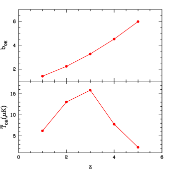
Figure 2.— The OHM clustering bias and the mean Rayleigh-Jeans temperature at z=1, 2, 3, 4 and 5. We find the OHM signal declines quickly when $z>3$.

We can now calculate the mean intensity of the OH emission:

$$\bar{I}_{\rm OH}(z)=f_{\rm OH}\int_{M_{\rm min}}^{M_{\rm max}}dM\frac{dn}{dM}f_{\rm IR}(M)\frac{L_{\rm OH}(M,z)}{4\pi D_{L}^{2}}y(z)D_{A}^{2},$$ (9)

where the $dn/dM$ is the halo mass function (Sheth & Tormen, 1999), $D_{L}$ and $D_{A}$ are the luminosity distance and comoving angular diameter distance respectively, and $y(z)=d\chi/d\nu=\lambda_{\rm OH}(1+z)^{2}/H(z)$, where $\chi$ is the comoving distance, $\nu$ is the observed frequency, $\lambda_{\rm OH}=18\ \rm cm$ is the rest-frame OH wavelength. The $f_{\rm OH}$ is the fraction of the LIRGs together with ULIRGs that host the OHMs. We set $f_{\rm OH}=0.2$ which is estimated using the sample in Darling & Giovanelli (2002). This takes account of the fact that the OHMs are caused by the far-IR pumping ($53\ \rm\mu m$) in the warm dust ($T>45\ \rm K$) which is produced and supported by the star formation in LIRGs or ULIRGs (Lockett & Elitzur, 2008). Note that the duty cycle does not appear in our formula, since it is already included in our SFR-$M$ relation.

Here we assume that the megamasers would dominate the contribution, so we can take $M_{\rm min}=10^{11}\ \rm M_{\odot}/h$, as the OHMs are hosted in galaxies with molecular gas $M_{\rm H_{2}}\gtrsim 4\times 10^{9}\ \rm M_{\odot}$ (Burdyuzha & Vikulov, 1990; Lagos et al., 2011; Duffy et al., 2011). The $f_{\rm IR}(M)$ is the fraction of the LIRGs and ULIRGs for galaxies hosted by the halos with $M>10^{11}\ \rm M_{\odot}/h$, which is estimated from the catalog in De Lucia et al. (2007). We find $f_{\rm IR}\sim 1$ when $M>1.2\times 10^{12}\ \rm M_{\odot}$, and quickly decreases for lower halo masses. After getting the OHM intensity, we can convert it into a mean Rayleigh-Jeans temperature $\bar{T}_{\rm OH}$.

The OHM clustering bias can be calculated in the same way as the HI bias (c.f. Eq. 5), except for the weight by $L_{\rm OH}$ instead of $M_{\rm HI}$. The OHM bias $b_{\rm OH}$ and $\bar{T}_{\rm OH}$ at z=1, 2, 3, 4 and 5 are shown in Fig. 2. We find that the OHM signal declines quickly when $z>3$.

The OHM power spectrum is given by $P_{\rm OH}(k,z)=\bar{I}_{\rm OH}^{2}b_{\rm OH}^{2}P(k,z)$, and similar to the HI case, the shot-noise power spectrum is given by

$$P_{\rm OH}^{\rm shot}(z) = f_{\rm OH}\int_{M_{\rm min}}^{M_{\rm max}}dM\frac{dn}{dM}$$ (10)

$$\times f_{\rm IR}(M)\left[\frac{L_{\rm OH}(M,z)}{4\pi D_{L}^{2}}y(z)D_{A}^{2}\right]^{2}.$$

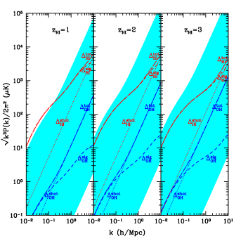
Figure 3.— The rms intensity fluctuations using the power spectrum of the OHM and 21-cm emission. The blue dashed, dotted and dash-dotted lines are the OHM signal, shot-noise and total power spectrum. The uncertainty of the OHM emission is also shown in cyan region, which is estimated using the errors in Eq.7 only. The red lines are 21-cm power spectrum. Because the shot-noise power spectrum is too small compared to the signal power spectrum for 21-cm, the total and the signal power spectrum are almost overlapped together.

3. Results and Discussion

In Fig. 3, we plot the rms fluctuations associated with the power spectrum of the OH and 21-cm emission at different redshifts for comparison. The 21-cm signal is plotted in red color, while the OH in blue. In the case of 21 cm power spectrum, the shot noise power is relativity insignificant, as the number of HI galaxies is large.

In the case of the OH power spectrum, the signal power spectrum evolves slowly in this redshift range, because the SFR is higher at high redshifts, so it counteracts the decrease in the matter power spectrum at high redshifts. The contribution of the shot noise is however very significant, especially at small scales (larger $k$), as the emission is mostly from the rare LIRG and ULIRG populations.

Comparing the 21cm power to the OH power, we find that on the scale of the first peak of the BAO (about $k=0.075h/{\rm Mpc}$), the OH rms fluctuations are about $0.03\%$, $0.07\%$ and $0.11\%$ of the 21 cm rms fluctuations at $z_{\rm HI}=1$, 2 and 3 respectively. At higher redshifts, while we do not show it here, we found that the 21cm signal become stronger as we approach the epoch of reionization, while the OH power become smaller and insignificant compared with the HI signal.

We note that this result depends on the modeling of the HI and OH emission, which still has a lot of uncertainty. The exact conditions for the occurrence of OH megamasers are not completely understood (Lo, 2005), and the actual OH emission from a source of a certain star formation rate may be quite different from our model prediction. Moreover, the OH emissivity may not even be strongly correlated with the halo mass, though on very large scales we still expect that the OH intensity power spectrum to be proportional to the underlying matter power spectrum. The 21 cm power depends on the HI content of the low mass halos, which is also largely uncertain.

Considering variations to our model predictions, we do find that in an extreme case, as shown the upper limit of the cyan region in Fig. 3, the OH could even supersede the 21cm power spectrum, and become the major contribution to the observed temperature fluctuations. Note that we just consider the errors in the $L_{\rm OH}$-$L_{\rm IR}$ relation (Eq. 7) to get the uncertainty (cyan region), which can be greater if including the error in $L_{\rm IR}$-SFR relation (Eq. 8). Also, we note that the two relations above are calibrated at low redshift and tightly related to the redshift-dependent properties of galaxies, such as the galaxy metallicity. So the OH intensity may also increase if considering the redshift evolution effect. Of course, in that case, it would be more advantageous to use the OH emission as the tracer instead, though at present this does not seem to be very likely.

As a lot of the OH power comes from shot noise, it may be possible to find a way to remove some of its contribution. For example, we may consider to conduct a targeted maser survey on the ULIRGs and LIRGs with sensitive telescopes which have small fields of view, and subtract their contributions to the temperature fluctuation. This could significantly reduce the noise power due to these sources.

One way to identify and estimate the amount of possible contamination is to cross correlate the temperature fluctuation at the redshift pair $(z_{1},z_{2})$. We expect the temperature fluctuations should be uncorrelated, while contamination by OH would give raise a correlation given by $\langle\delta T(k,z_{1})\delta T(k,z_{2})\rangle=b_{\rm HI}(z_{2})b_{\rm OH}(z_{2})P(k,z_{2})$.

Finally, it may also be possible to make use of the multiple lines of OH (including the four lines at 18cm and the lines with shorter wavelengths) to check for the contamination. If observations for individual OHM sources show that most of them have similar line ratios, then one may construct a template of OHM spectrum, and apply it as a matched filter on the observed spectrum to check for possible OH contamination. However, this would not be possible if observations show that the line ratios vary a lot.

We thank Prof. Xingwu Zheng for helpful discussion. This work was supported by NSF CAREER AST-0645427 at UCI, by the 973 program No. 2007CB815401, the NSFC grant No.11073024, and the John Templeton Foundation at NAOC; and MGS and MBS acknowledges support from FCT Portugal under grant PTDC/FIS/100170/2008.

References

- Ansari et al. (2008) Ansari, R. et al., 2008, arxiv:0807.3614
- Aretxaga et al. (2007) Aretxaga, I. et al., 2007, MNRAS, 379, 1571
- Bann (1989) Baan, W. A. 1989, ApJ, 338, 804
- Burdyuzha & Vikulov (1990) Burdyuzha, V.V. & Vikulov, K.A. 1990, MNRAS, 244, 86
- Carilli (2011) Carilli, C., 2011, ApJ, 730, 30.
- Chang et al. (2008) Chang, T., Pen, U., Peterson, J. B., McDonald, P., 2008, Phys. Rev. Lett., 100, 091303.
- Chang et al. (2010) Chang, T., Pen, U., Bandura, K., Peterson, J. B., 2010, Nature, 466, 463.
- Conroy & Wechsler (2009) Conroy, C. & Wechsler, R. H. 2009, ApJ, 696, 620
- Darling & Giovanelli (2002) Darling, J. & Giovanelli, R. 2002, AJ, 124, 100
- De Lucia et al. (2007) De Lucia, G. et al., 2007, MNRAS, 375, 2
- Duffy et al. (2011) Duffy, A. R., Kay, S. T., Battye, R. A., Booth, C. M.,Vecchia, C. D. & Schaye, J. 2011, arXiv:1107.3720
- Evans et al. (2006) Evans, A. S., Solomon, P. M., Tacconi, L. J. & Downes, D. 2006, ApJ, 132, 2398
- Gong et al. (2011) Gong, Y., et al. 2011, ApJ, 728, L46
- Gong et al. (2011b) Gong, Y., et al. 2011b, arXiv:1107.3553
- Kandalian (1996) Kandalian, R. A. 1996, 39, 237
- Kennicutt (1998) Kennicutt, R. C. 1998, ARAA, 36,189
- Klckner (2004) Klckner, H.-R. 2004, PhD Thesis, University of Groningen
- Komatsu et al. (2011) Komatsu, E., et al. 2011, ApJS, 192,18
- Lagos et al. (2011) Lagos, C. P., Baugh, C. M., Lacey, C. G., Benson, A. J. Kim, H. & Power, C. 2011, arXiv:1105.2294
- Lah et al. (2007) Lah, P., et al. 2007, MNRAS, 376, 1357
- Lidz et al. (2011) Lidz, A., et al. 2011, arXiv:1104:4800
- Lo (2005) Lo, K. Y., 2005, ARA&A, 43, 625.
- Lockett & Elitzur (2008) Lockett, P. & Elitzur, M. 2008, ApJ, 677, 985
- Loeb & Barkana (2001) Loeb, A., & Barkana, R. 2001, ARA&A, 39, 19
- Loeb et al. (2005) Loeb, A., Barkana, R. & Hernquist, L. 2005, ApJ, 620, 553
- Magnelli et al. (2011) Magnelli, B., et al. 2011, arXiv:1101.2467
- Marin et al. (2010) Marin, F. A., Gnedin, N. Y., Seo, H. & Vallinotto, A. 2010, ApJ, 718, 972
- Noterdaeme et al. (2009) Noterdaeme, P., Petitjean, P., Ledoux, C. & Srianand, R. 2009, A&A, 505, 1087
- Obreschkow et al. (2009) Obreschkow D., et al. 2009, ApJ, 703, 1890
- Peterson et al. (2009) Peterson, J. B. et al., 2009, arxiv:0902.3091
- Randell et al. (1995) Randell, J., Field, D., Jones, K. N., Yates, J. A. & Gray, M. D. 1995, A&A, 300, 659
- Rao et al. (2006) Rao, S. M., Turnshek, D. A. & Nestor, D. B. 2006, ApJ, 636, 610
- Santos et al. (2008) Santos, M. G. et al., 2008, ApJ, 689, 1
- Seo et al. (2010) Seo, H. J. et al., 2010, ApJ, 721, 164.
- Sheth & Tormen (1999) Sheth, R. K., & Tormen, G. 1999, MNRAS, 308, 119
- Shimasaku et al. (2008) Shimasaku, K., Hayashi, M., Motohara, K., et al. 2008, ASP Conf. Ser., 399, 75
- Smith et al. (2003) Smith, R. E., et al. 2003, MNRAS, 341, 1311
- Springel et al. (2005) Springel, V., et al. 2005, Nature, 435, 629
- Tekola et al. (2011) Tekola, A. G., Vaisanen, P., & Berlind, A. 2011, arXiv:1101.3495
- Thompson, Moran & Swenson (2001) Thompson, A. R., Moran, J. M., Swenson, G. W. Jr., 2001, Interferometry and Synthesis in Radio Astronomy, John Wiley & Sons Inc., New York.
- Visbal & Loeb (2010) Visbal, E. & Loeb, A. 2010, JCAP, 11, 016