Structure and Turbulence in Simulated Galaxy Clusters and the Implications for the Formation of Radio Halos

Abstract

We track the histories of massive clusters of galaxies formed within a cosmological hydrodynamic simulation. Specifically, we track the time evolution of the energy in random bulk motions of the intracluster medium and X-ray measures of cluster structure and their relationship to cluster mergers. We aim to assess the viability of the turbulent re-acceleration model for the generation of giant radio halos by comparing the level of turbulent kinetic energy in simulated clusters with the observed properties of radio halo clusters, giving particular attention to the association of radio halos to clusters with disturbed X-ray structures. The evolution of X-ray cluster structure and turbulence kinetic energy, $k$, in simulations can then inform us about the expected lifetime of radio halos and the fraction of clusters as a function of redshift expected to host them. We find strong statistical correlation of disturbed structure measures and the presence of enhancements in $k$. Specifically, quantitatively “disturbed”, radio halo-like X-ray morphology in our sample indicates a 92% chance of the cluster in question having $k$ elevated to more than twice its minimum value over the cluster’s life. The typical lifetime of episodes of elevated turbulence is on the order of 1 Gyr, though these periods can last 5 Gyrs or more. This variation reflects the wide range of cluster histories; while some clusters undergo complex and repeated mergers spending a majority of their time in elevated $k$ states, other clusters are relaxed over nearly their entire history. We do not find a bimodal relationship between cluster X-ray luminosity and the total energy in turbulence that might account directly for a bimodal $L_{X}-P_{1.4GHz}$ relation. However, our result may be consistent with the observed bimodality, as here we are not including a full treatment of cosmic rays sources and magnetic fields.

1 INTRODUCTION

Galaxy clusters have long been known as radio synchrotron sources. Given that observations show that the intracluster medium is typically magnetized at the $\sim$$\mu G$ level (see Carilli & Taylor, 2002; Govoni & Feretti, 2004), what is required for the radio emission is a nonthermal population of accelerated electrons. Arguments for various scenarios responsible for cluster radio emission therefore hinge on the method of particle acceleration, using the observed radio and X-ray properties of galaxy clusters as discriminatory evidence. Radio properties of the sources in galaxy clusters vary, though in general the types of sources can be separated into two basic categories, sources associated with individual galaxies and those associated with the diffuse intracluster medium (ICM). Those associated to individual galaxies include the jet and lobe sources connected to active galactic nuclei (AGN) (e.g., Hardcastle et al., 2003; Nulsen et al., 2005). The diffuse sources can be further divided into two broad classes, radio relics and radio halos. Radio relics include both steep spectrum re-energized AGN jet lobes, as well as polarized sources likely associated with recently accelerated cosmic-ray (CR) electrons at merger shocks (e.g., Clarke & Ensslin, 2006; van Weeren et al., 2010). These extended, elongated features are steep spectrum sources with curved shapes, spatially distinct and strongly argued as coincident with shocks from both observations and numerical simulations (Roettiger et al., 1999; Kassim et al., 2001; Bagchi et al., 2006; Skillman et al., 2010). Radio halos (RHs), by contrast, are Mpc-scale, diffuse, unpolarized, steep spectrum radio emitting regions typically centered on the X-ray center of the ICM, with a spatial distribution similar to the X-ray emission (Liang et al., 2000; Feretti et al., 2001; Giacintucci et al., 2009; Macario et al., 2010).

The origin of RHs is less certain than the radio relics, though it was recognized a decade ago (e.g. Buote, 2001), and observational evidence now continues to suggest that they are associated with merging clusters (Sarazin, 2004; Govoni et al., 2004; Brunetti et al., 2009; Cassano et al., 2010). For example, the recent work of Cassano et al. (2010) uses radio observations (with GMRT) and Chandra observations of an X-ray selected sample of galaxy clusters to make a strong case for a division in the observed X-ray morphological properties of RH and non-RH galaxy clusters. In brief, clusters that are more disturbed in the X-ray power ratios, centroid shift measures and have lower concentration parameters are those that tend to host radio halos. Those with relaxed structure measures and higher concentrations tend to not have detectable large-scale radio emission.

Recent observational and simulation work argues that RHs are created through merger-induced turbulent re-acceleration of an existing population of CRs in the ICM. The argument for turbulent re-acceleration of a pre-existing CR electron population as the cause of RHs appeals to a combination of observational properties. First, the radio emission is broadly distributed over a relatively large volume, roughly centered on the X-ray centroid of the cluster, and more or less spatially uniform (for a recent review, see Ferrari et al., 2008). Given the short synchrotron lifetimes of the CR electrons responsible for the emission, they must be accelerated in situ, ruling out acceleration from large individual shock structures on morphological grounds (Brunetti et al., 2001). Turbulence provides a source of energy that is distributed relatively evenly over the cluster volume. Second, this model naturally explains the connection of the presence of RHs to cluster mergers. Though second order Fermi processes are usually invoked (Petrosian, 2001), there are legitimate questions about the exact method by which the turbulent energy can be converted into accelerated particles. In addition, a key prediction of the turbulent re-acceleration model is the expected presence of very steep spectrum RHs ($\alpha>1.6$) (Cassano, 2009). Two recent RHs have been found to host so called ultra steep spectrum radio halos, A521 (Brunetti et al., 2008) and A697 (Macario et al., 2010). These discoveries, though small in number so far, fit the turbulent re-acceleration model.

Another explanation proposed for the origin of RHs is hadronic production. This model invokes the production of secondary relativistic electrons generated by the collisions of relativistic protons and the thermal population of atomic nuclei in the ICM. In the hadronic scenario, the secondary electrons are responsible for the observed radio emission (e.g., Pfrommer et al., 2008; Keshet & Loeb, 2010; Keshet, 2010), and the proponents argue that the hadronic model more naturally explains the correlation of the radio emission with the X-ray emitting ICM (i.e. the target population for p-p collisions) and the presence of both RHs and radio relics in clusters. Merger induced enhancement of cluster magnetic fields is invoked to explain the RH-merger connection (Kushnir et al., 2009; Keshet & Loeb, 2010). However, recent $\gamma$-ray upper limits from Fermi observations of galaxy clusters are beginning to constrain the capability of hadronic models to account for RHs (see Jeltema & Profumo, 2011), as the hadronic processes should also generate $\gamma$-rays from neutral pion decay. The recent discovery of ultra steep spectrum radio sources described above is also not predicted in the hadronic scenario given the energetic considerations required by the $\gamma$-ray upper limits. These and other constraints suggested by observations of RHs, such as the spectral and spatial properties of the radio emission (see Brunetti, 2004), argue against the hadronic model.

One more piece of observational evidence in the case of radio halos is the relationship between the bulk X-ray and radio properties of massive galaxy clusters. The radio luminosity at 1.4$GHz$ and the X-ray luminosity of massive radio halo galaxy clusters exhibit a strong correlation for many objects. However, there apparently exists a bimodal distribution in the $L_{x}-P_{1.4GHz}$ plane, where many clusters have no radio detections, only upper limits in $P_{1.4GHz}$ that lie well below the scaling relation. These objects are of similar mass and X-ray luminosity to those that clearly host radio halos and are on the scaling relation. There is a significant gap between the measured radio luminosity of the RHs and the upper limits of the non-RH objects, which suggests that the transition between the two phases (radio halo versus non-RH) must be relatively quick (Brunetti et al., 2009). While there were initial concerns that the bimodality of the $L_{x}-P_{1.4GHz}$ relation might be an artifact of selection effects (e.g., Rudnick & Lemmerman, 2009), the depth of the radio data for the current samples appears to address that issue. The presence of a strong correlation of radio power with X-ray luminosity for RH clusters, the bimodality of the relation, and the inferred lifetime and transition times for RHs have been used to argue for or against models of radio halo production (e.g. Kushnir et al., 2009; Brunetti et al., 2009). In this case, numerical simulations provide a window into the evolution of the relevant physical properties of the ICM.

In this paper, we study the evolution over time of massive clusters formed within a cosmological volume simulation, which allows us to track cluster mergers, the evolution of cluster structure, and the presence and evolution of turbulence. Using simulations, we can investigate the frequency and timescale over which clusters exhibit elevated levels of turbulence and X-ray structures similar to those observed for RH clusters. The use of cosmological simulations turns out to be critical to accurately capture cluster merger histories. In particular, we attempt to understand the connection between the X-ray morphology of galaxy clusters and the putative energy source for CR acceleration in the ICM: turbulence. We do not attempt to determine the method of particle acceleration, we merely discuss the probability of the turbulent re-acceleration model of RHs given the correlations between the physical properties of the simulated clusters and their observed morphological characteristics. We study both the “snapshot” correlations for our clusters between the X-ray structure measures (power ratios and centroid shifts) and the turbulence kinetic energy and the time evolution of these properties.

Section 2 of this paper describes the methodology of the analysis we undertake, including the details of the numerical simulations and analysis and the method of calculating the X-ray structure measures from the synthetic observations. Section 3 describes the distribution of simulated galaxy cluster structures compared to observations, the time evolution of both the structure measures and turbulence kinetic energy, and compares how the turbulence kinetic energy correlates with the observed properties of radio halo clusters. Section 4 gives estimates for lifetimes and duty cycles for radio halos based on the typical duration of episodes of elevated turbulence kinetic energy and the fraction of clusters in these states. Section 5 summarizes and discusses the implications of our results.

2 METHODOLOGY

2.1 Simulations

For this study we use a numerical cosmological hydrodynamic/N-body simulation generated using the Enzo code, a publicly available adaptive mesh refinement (AMR) cosmology code developed by Greg Bryan and colleagues (Bryan & Norman, 1997a, b; Norman & Bryan, 1999; O’Shea et al., 2004, 2005). The specifics of the Enzo code are described in detail in these papers (and references therein).

This simulation is set up as follows. We initialize our calculation at $z=99$ assuming a cosmological model with $\Omega_{m}=0.27$, $\Omega_{b}=0.04$, $\Omega_{\Lambda}=0.73$, $h=0.7$ (in units of 100 km/s/Mpc), $\sigma_{8}=0.9$, and using an Eisenstein & Hu (1999) power spectrum with a spectral index of $n_{s}=0.97$. The simulation is of a volume of the universe 128 h^-1 Mpc (comoving) on a side with a $256^{3}$ root grid. The dark matter particle mass is $9.1\times 10^{9}$ h^-1 M_⊙. The simulation was then evolved to $z=0$ with a maximum of $5$ levels of adaptive mesh refinement (a maximum spatial resolution of $15.6$ h^-1 comoving kpc), refining on dark matter and baryon overdensities of $8.0$.

This simulation includes a prescription for radiative cooling of the gas using non-equilibrium cooling and chemistry for H and He, and a spatially uniform but time-varying Haardt-Madau ultraviolet radiation background. In this case, we have not included metal line cooling as has been done in previous calculations, since in this study we are interested in the morphological properties of the clusters. Many investigators have documented the over-cooling problems associated with including metal cooling in cosmological simulations, and in previous work we have shown that this over-cooling leads to a severe mismatch of structure measures between the observed and simulated cluster images.

We perform all our post-processing analysis for this work using the YT analysis toolkit (Turk et al., 2011). For each of 132 simulation outputs equally spaced in time ($\delta t$ = 0.055 Gyr) in the redshift interval 0 $\leq z\leq$0.9, we ran the HOP halo-finding algorithm (Eisenstein & Hut, 1998) on the dark matter particle distribution to produce a dark matter halo catalog. For each halo catalog in each time interval, we create spherically averaged radial profiles of a set of physical properties (including density and mass) to calculate the value of $r_{200}$ and $M_{200}$ for the identified halos. $M_{200}$ refers to the total mass inside a radius of $r_{200}$, the radius at which the overdensity average inside the sphere centered on the cluster is 200 times the critical density. We then took all the halos at $z$=0 with $M_{200}\geq 3\times 10^{14}M_{\odot}$ (a relatively arbitrary cutoff) as our sample. We choose the high mass objects so that we can make a reasonable comparison to the very high mass objects of Cassano et al. (2010), and to limit our sample to the best resolved objects in the simulation. This cut results in a sample at $z$=0 of 16 galaxy clusters.

Following the identification of the sample, we generated a set of synthetic 0.3-8.0 keV X-ray images of each cluster generated from the Cloudy software (Ferland et al., 1998). We then make a corresponding image of each of these clusters from each of the 132 time outputs described above. Each initial image represents a projected area of 8 by 8 Mpc around each cluster in order to study both the cluster and the surrounding structures. The X-ray images are output in FITS format with the correct angular scale for their redshift, and with the flux modified by the distance. Therefore, we are left with a series of synthetic X-ray surface brightness images that we can analyze in a similar way to observed images of galaxy clusters. Each series represents a time history of each of our 16 clusters. Additionally, we have calculated the bulk properties of each cluster and its most massive predecessors throughout this time history.

2.2 Structure Measures and Turbulence

2.2.1 Structure Measures

The association of radio halos with clusters undergoing mergers, known visually for quite some time, has been established quantitatively through the presence of significant substructure or disturbed cluster structure in the X-ray surface brightness distribution (e.g. Buote, 2001; Cassano et al., 2010). In particular, Cassano et al. (2010) use three structure measures based on X-ray images of the clusters in their sample: the centroid shift $w$, the third order power ratio $P_{3}/P_{0}$, and the concentration $c$. Cassano et al. (2010) show that giant radio halo clusters can be efficiently separated from non-radio halo clusters and radio mini-halos in the plane defined by any two of these structure measures (i.e. $w$ vs. $P_{3}/P_{0}$, $c$ vs. $w$, or $c$ vs. $P_{3}/P_{0}$).

Here we will employ the former two statistics, the centroid shift and $P_{3}/P_{0}$, the calculations of which have been discussed in detail in previous papers (Jeltema et al., 2005, 2008; Hallman et al., 2010). In brief, the centroid shift measures the variation (here standard deviation) of the position of the centroid of the X-ray surface brightness of a cluster relative to the X-ray peak in apertures of increasing radius, and w is normalized relative to the largest aperture considered. The power ratios are based on the multipole moments of the X-ray surface brightness in an aperture of a given size; specifically they are proportional to the sum of the squares of the moments divided by the total cluster flux (Buote & Tsai, 1995). $P_{3}/P_{0}$ is the third order power ratio and is sensitive to deviations from mirror symmetry. For consistency with Cassano et al. (2010), we employ the same overall aperture size of 500 kpc for both $w$ and $P_{3}/P_{0}$ as well as the same aperture spacing of 25 kpc for the centroid shift (see for example equations 1-5 in Cassano et al. (2010)). In the case of the centroid shift, we remove the central 50 kpc surrounding the X-ray peak from consideration. The centroid shift $w$ and the power ratios within an aperture of 500 kpc are calculated for every time output over the history of our 16 simulated clusters.

We do not use the concentration parameter, which is defined by Cassano et al. (2010) as the ratio of the X-ray surface brightness within the central 100 kpc to the surface brightness within 500 kpc. With this definition, the typical cluster concentration evolves significantly with redshift as a fixed 100 kpc aperture encloses more or less of the cluster volume. This evolution makes a fixed cut for relaxed or disturbed clusters impossible. A different definition of concentration based on overdensity radii would provide a better criterion for clusters spanning a large redshift range but would not allow a direct comparison to the observed radio halo sample of Cassano et al. (2010). We note, however, that in the redshift range spanned by the Cassano et al. (2010) sample, we find a similar median concentration for our simulated clusters to that of the observed clusters once the X-ray peak is removed (as was done for the centroid shifts).

2.2.2 Turbulence Kinetic Energy

To evaluate the connection between the morphological structure measures and the physical state of the cluster, we have made a calculation of the mass-averaged turbulence kinetic energy (TKE) for each cluster inside the same radius (500 kpc) that we have calculated the structure measures. Here we use a common definition of the turbulence kinetic energy density (see e.g., Choudhuri, 1998)

$$k=0.5(\overline{u_{x}^{2}}+\overline{u_{y}^{2}}+\overline{u_{z}^{2}}),$$ (1)

where $u_{x},u_{y},u_{z}$ are the orthogonal components of the peculiar velocity of the gas in each grid zone (subtracting the bulk halo velocity), and $k$ is the specific kinetic energy. The bulk halo velocity is calculated as the mass-weighted average velocity of all dark matter particles identified by the halo finding algorithm as halo members. For our analysis we calculate a mass-averaged value of $k$ in a sphere with $r$=500 kpc around each cluster center. We note that we are not truly calculating the energy of the full turbulent cascade. We can calculate a physical Reynolds number for flows of characteristic length scale equal to the minimum grid scale (for grid elements at the peak spatial resolution) of the simulation. Our grid size at peak spatial resolution and the characteristic parameters of the ICM flows can be combined into a dimensionless Reynolds number

$$Re=vL/\nu,$$ (2)

where $v$ is the fluid velocity, $L$ is a characteristic length, and $\nu$ is the kinematic viscosity of the fluid. We can estimate the values for $v$ and $L$ to be roughly the sound speed $c_{s}$ and minimum grid scale. Estimates of the viscosity are trickier, but the viscosity for a fully ionized unmagnetized thermal plasma (Braginskii, 1958; Spitzer, 1962) can be written as

$$\mu_{um}=2.2\times 10^{-15}\frac{T^{5/2}}{ln\Lambda}gcm^{-1}s^{-1}.$$ (3)

For typical values of the ICM temperature ($kT\approx$10 keV) and density and assuming a sound speed of $c_{s}$=1000 km/s, the Reynolds number at our peak grid resolution is roughly $Re\approx 250$. Flows with these Reynolds numbers are below the expected threshold for transition from laminar to turbulent flow in an ideal gas. Additionally, for our simulations, the details of turbulent flow (should it exist) are not captured at our smallest grid scale or below. However, $Re$ scales linearly with the characteristic length of the flow, and large scale eddies should be captured. We expect that turbulence injection in the ICM happens at scales well above our grid size ($L\approx 100-400kpc$) (Brunetti & Lazarian, 2011). What we do capture in this calculation is the kinetic energy associated with bulk random motions of the ICM gas at and above the grid scale of the simulation. This motion would be converted to thermal energy through the turbulent cascade (and through shock dissipation) in the real ICM. So this calculation is made to simply characterize the available energy in random bulk motion of the ICM, which we assume will eventually be dissipated into heat (and possibly CRs) through the turbulent cascade. Indeed, recent work by Paul et al. (2011) indicates that our metric $k$ should be relatively insensitive to the spatial resolution of the simulation grid.

The quantity $k$ is tracked with time in the history of each cluster to determine the change in the TKE. If the paradigm that cluster radio halos are powered by turbulent re-acceleration of CRs is correct, increases in the TKE should lead to an increase in the radio brightness. Therefore, we can make estimates of the lifetime of radio halos by tracking the TKE evolution. We also study the correlation of the X-ray structure measures with the TKE; since the presence of a radio halo is observed to be linked to X-ray structure, the TKE should likewise be correlated to cluster structure if indeed turbulence is connected to the production of radio halos.

3 CONNECTION OF CLUSTER MERGERS, STRUCTURE, AND TURBULENCE

3.1 Distribution of Cluster Structures

Cassano et al. (2010) show that radio halo clusters can be distinguished from non-radio halo clusters based on their observed X-ray structure. In particular, in terms of the two structure measures we consider, Cassano et al. (2010) find that clusters hosting radio halos tend to lie in the upper-right quadrant of the $w-P_{3}/P_{0}$ plane with high centroid shifts and high $P_{3}/P_{0}$. Below, we compare the distribution of clusters structures for our simulated clusters to observed clusters from the Cassano et al. (2010) sample and show that they are similar.

In Figure 1, we show the distribution of structures of our simulated clusters in the $w-P_{3}/P_{0}$ plane for all time outputs with $0.2\leq z\leq 0.4$, the redshift range spanned by the Cassano et al. (2010) sample. Cassano et al. (2010) make cuts for radio halo versus non-halo clusters based on the median of each structure measure, which for their sample gives $w=0.012$ and $P_{3}/P_{0}=1.2\times 10^{-7}$. Most of the radio halo clusters in their sample do in fact have $w>0.012$ and $P_{3}/P_{0}>1.2\times 10^{-7}$. For our simulated sample in a similar redshift range ($0.2\leq z\leq 0.4$), we find median values of $w=0.010$ and $P_{3}/P_{0}=4.6\times 10^{-8}$, similar particularly for the centroid shift to the Cassano et al. (2010) values. Both the Cassano et al. (2010) structure cuts (red lines) and the median values in the simulations (black lines) are shown in Figure 1. We find that in the $0.2\leq z\leq 0.4$ redshift range, $24\%$ of the simulated cluster images have structures above the Cassano et al. (2010) cuts ($w>0.012$ and $P_{3}/P_{0}>1.2\times 10^{-7}$) while $36\%$ have structures above the median values for the simulated sample.

Overall there is a good match between the structure of clusters in our simulations and observed clusters in terms of both the typical cluster structure and range of structure measures. Comparing Figure 1 to Figure 1 in Cassano et al. (2010) gives the visual impression that a larger fraction of simulated clusters lie in the off-diagonal (lower-right and upper-left) regions of the structure plane implying a less strong correlation of $w$ and $P_{3}/P_{0}$. In Figure 1, a total of $26-28\%$ (depending on the cuts used) of the simulated cluster images lie in the two off-diagonal quadrants compared to 5 out of 32 in the Cassano et al. (2010) sample, not a significant difference given the sample size.

The fraction of simulated clusters in the upper-right quadrant of the $w-P_{3}/P_{0}$ plane, which have X-ray structures similar to those observed for radio halo clusters, is a good match to the $29\pm 9\%$ of X-ray luminous clusters found to host radio halos in the survey of a complete cluster sample with the Giant Meterwave Radio Telescope (GMRT) (Venturi et al., 2008) (from which the Cassano et al. (2010) sample is drawn) and to the 12 out of 32 clusters hosting giant radio halos in the Cassano et al. (2010) sample.

If we consider instead the full redshift range of the simulations ($0.0\leq z\leq 0.9$), we find that clusters have radio halo like structures $19\%$ ($31\%$) of the time given the Cassano et al. (2010) (simulated) structure cuts. As we will show in later sections, some clusters spend most of their time in disturbed states while other clusters are relaxed over nearly all of their history.

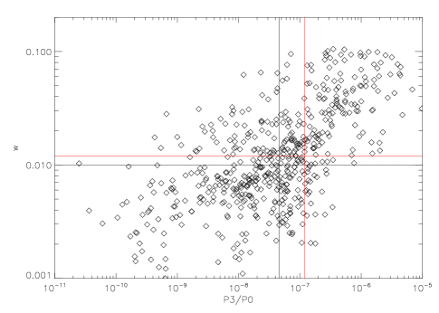
Figure 1: The centroid shift $w$ versus $P_{3}/P_{0}$ plane for all the simulated cluster images in the redshift range $0.2\leq z\leq 0.4$ (the range in Cassano et al. (2010)). Red lines indicate the structure cuts from Cassano et al. (2010), black are the median values for our simulated clusters.

3.2 Cluster Histories

We follow the evolution of both the structure measures and the TKE for individual simulated clusters through time. This reveals a wide range of cluster histories. We investigate the effect of mergers on measured cluster structure (i.e. the observable effects of mergers) and on the TKE. We can then ask when clusters have structure measures similar to those observed for radio halos and how this relates to the TKE and merger history.

The time histories of the TKE in 6 of the simulated clusters in our sample are shown in Figure 2. The clusters are chosen to represent a wide range of time histories. We use the kinetic energy density as defined earlier to remove the effect of increasing mass on the result. In each case, for the purposes of comparison with the structure measures, we only examine the value of $k$ inside a radius of 500 kpc. It is clear from these histories that the value of $k$ undergoes major variations as a function of time in each cluster. These variations can change the value by factors of 5 or more over time intervals of 0.5-1 Gyr. The strong increases in the TKE will be shown in later sections to correspond directly to the incidence of merging events. These merging events, as has been shown in previous investigations, also correspond to changes in the X-ray structure measures.

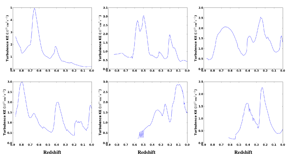
Figure 2: A sample of the turbulence kinetic energy (TKE) density histories for 6 of the simulated clusters. These show the wide range of features exhibited by the time evolution of the TKE. Note the vertical scale differs across the plots.

However, for the structure measures, the variations with time for individual clusters are not as smooth as those for the TKE. Figure 3 shows the variation in the $P_{3}/P_{0}$ power ratio as a function of redshift for the same 6 simulated clusters shown in Figure 2. While the TKE rises and falls smoothly during merger events, the value of the X-ray $P_{3}/P_{0}$ power ratio jumps up and down significantly during the whole life of the cluster. From previous studies, we were aware that the power ratios can vary significantly on short time scales. Merger phase can have a strong effect on the structure measures. Strong dips in $P_{3}/P_{0}$ are often seen, for example, at the moment of core passage in major mergers. The X-ray structure measures tend to be highest in the pre-merger and post-core passage re-expansion phases when subclusters are well-separated and/or asymmetric features are most prominent. Statistically, X-ray structure measures like $w$ and $P_{3}/P_{0}$ correlate strongly with cluster dynamical state, but significant scatter is present for individual cluster measurements (projection effects also contribute to the scatter) (Jeltema et al., 2008). Therefore, though a correlation between the turbulence kinetic energy and the X-ray structure measures is expected, it is not immediately obvious from individual cluster time histories that this is the case.

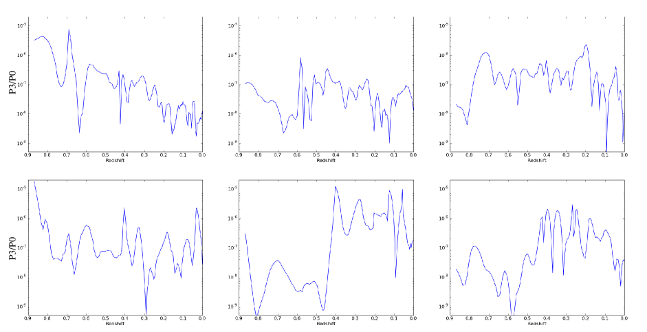
Figure 3: A sample of the X-ray $P_{3}/P_{0}$ histories for the same 6 simulated clusters for which we plotted TKE histories in Figure 2. Note the wide variation of $P_{3}/P_{0}$ on short time scales compared to the smooth variation of the TKE.

To further illuminate the effects of cluster mergers, in Figures 4, 5, and 6 we show three example mergers from our simulated cluster sample which exhibit quite varied merger progessions. During the mergers, we have measured the value of both $\langle w\rangle$ and $P_{3}/P_{0}$, as well as the turbulence kinetic energy $k$. In each figure, the images from left to right in both the upper and second row are a time series of X-ray surface brightness (upper) and X-ray weighted temperature (second). The two plots in the second row from the bottom show the progression in time of the TKE (left) and the position in the $P_{3}/P_{0}$-$\langle w\rangle$ plane. The bottom panels show the evolution of the individual structure measures as a function of redshift. Letters indicate the position in the time series. In Figure 4, we see in panel A a subhalo approaching the main cluster; in panel B, this subcluster is driving an obvious large shock into the gas. Point B in the TKE time series is associated with the peak of the enhancement, and also the structure measures have moved into the disturbed area of the $P_{3}/P_{0}$-$\langle w\rangle$ plane. As the subcluster passes through the main cluster, the TKE declines gradually, and the structure measures move back into the “relaxed” regions of the structure plot. Between points B and C, the structure measures show the typical progression seen in cluster mergers: both $P_{3}/P_{0}$ and $\langle w\rangle$ show a peak near point B when the subcluster enters the 500 kpc aperture; as the cluster undergoes core passage between points B and C, the structure measures both dip; $P_{3}/P_{0}$ and $\langle w\rangle$ then show a second peak following core passage in the re-expansion phase before declining again. Point C is near the end of re-expansion and outgoing shocks can be seen in the temperature map. Compared to the structure measures, the TKE evolves smoothly throughout the merger. At point D, the small remaining core of the subcluster can been seen re-entering the cluster, but this more minor event does not lead to as large a rise in the structure measures or the TKE.

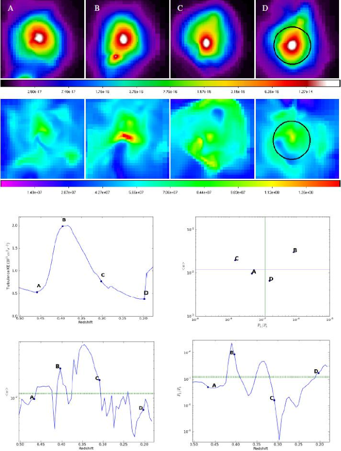
Figure 4: Merger snapshots for a simulated galaxy cluster in our sample. Upper panels show images of the synthetic 0.3-8.0 keV X-ray surface brightness while the panels immediately below show the projected X-ray weighted temperature. Image panels are roughly 1 kpc across. The black circle overlaid on the final time step indicates the fiducial 500 kpc radius used in our analysis for that timestep. The panels in the third row show the time evolution of the turbulence kinetic energy (left) and the location of the cluster in the $P_{3}/P_{0}-\langle w\rangle$ plane for the four time snapshots as indicated by letter. Bottom panels show the time evolution of $P_{3}/P_{0}$ and $\langle w\rangle$ with redshift; green dashed lines indicate the structure cuts used by Cassano et al. (2010) to select radio halo clusters. The mass of the main cluster ranges from 4.0$\times 10^{14}M_{\odot}$ at (A) to 5.0$\times 10^{14}M_{\odot}$ at (D).

Figure 5 shows a slightly more complicated merger. First, we have two approaching subclusters (seen in the upper center and upper right of panel A). The first merger drives a large shock, seen in the temperature image of panel B. This again leads to a spike in the TKE and a movement of the structure measures in to the disturbed regime. Before the cluster can relax, the second, apparently smaller subcluster plunges in, enhancing the TKE again and again boosting the structure measures toward the disturbed regime (point C). After an extended period, the TKE declines and the structure measures move in to the relaxed quadrant of the $P_{3}/P_{0}-\langle w\rangle$ plane (point D).

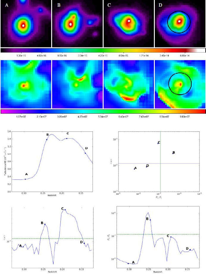
Figure 5: Merger snapshots for a simulated galaxy cluster in our sample. Upper panels show images of the synthetic 0.3-8.0 keV X-ray surface brightness while the panels immediately below show the projected X-ray weighted temperature. Image panels are roughly 1 kpc across. The black circle overlaid on the final time step indicates the fiducial 500 kpc radius used in our analysis for that timestep. The panels in the third row show the time evolution of the turbulence kinetic energy (left) and the location of the cluster in the $P_{3}/P_{0}-\langle w\rangle$ plane for the four time snapshots as indicated by letter. Bottom panels show the time evolution of $P_{3}/P_{0}$ and $\langle w\rangle$ with redshift; green dashed lines indicate the structure cuts used by Cassano et al. (2010) to select radio halo clusters. The mass of the main cluster ranges from 2.8$\times 10^{14}M_{\odot}$ at (A) to 3.5$\times 10^{14}M_{\odot}$ at (D).

Figure 6 shows a very complex scenario. In panel A we see two subhalos in the center left of the image which are in the process of merging. In panel B, the subhalos have merged with each other and are in a re-expansion phase (note the merger shock in the temperature image of panel A, and the outgoing shocks in B). They then pass by the main cluster on either side, with the leading shock sweeping over the main cluster. Meanwhile, in panel C, note another approaching subcluster to the upper right, which by panel D has plunged into the main cluster. This multiple merger, as seen in the context of the TKE and structure measures, has an increase in $k$ during both merger events, while the structure measures remain high throughout. This is a very dynamic environment, where multiple mergers take place throughout the cluster lifetime, leading to long periods of elevated TKE and disturbed structure measures.

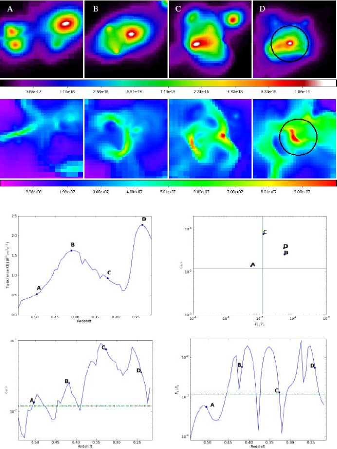
Figure 6: Merger snapshots for a simulated galaxy cluster in our sample. Upper panels show images of the synthetic 0.3-8.0 keV X-ray surface brightness while the panels immediately below show the projected X-ray weighted temperature. Image panels are roughly 1 kpc across. The black circle overlaid on the final time step indicates the fiducial 500 kpc radius used in our analysis for that timestep. The panels in the third row show the time evolution of the turbulence kinetic energy (left) and the location of the cluster in the $P_{3}/P_{0}-\langle w\rangle$ plane for the four time snapshots as indicated by letter. Bottom panels show the time evolution of $P_{3}/P_{0}$ and $\langle w\rangle$ with redshift; green dashed lines indicate the structure cuts used by Cassano et al. (2010) to select radio halo clusters. The mass of the main cluster ranges from a very small 1.6$\times 10^{14}M_{\odot}$ at (A) to more than double its original mass, 3.5$\times 10^{14}M_{\odot}$ at (D).

In general, we find that there is no ”typical” cluster history. Some clusters undergo complex mergers or progressions of successive mergers leading them to be disturbed over most of their history, while other clusters are nearly always relaxed, experiencing only one or two minor mergers from $z=0.9$ to the present. This diversity highlights the importance of using cosmological scale simulations, since idealized mergers would not capture the full complexity of cluster evolution.

3.3 Assessing the Turbulent Re-Acceleration Model

It is clear from the cluster histories that the TKE can increase drastically during cluster mergers (as you would expect) and that clusters can display quite different TKE evolutionary histories. In this section, we consider how the TKE correlates with the observed properties of radio halo clusters and if this is consistent with the turbulent re-acceleration model of radio halo production. Specifically, we examine the TKE in clusters with and without X-ray structures consistent with those observed for radio halo clusters, and we look at the correlation between total TKE and cluster X-ray luminosity.

3.3.1 Correlation of Cluster Structure and Turbulence

One of the main relevant questions of our investigation is whether the presence of enhanced TKE correlates with the value of the structure measures for the X-ray images. We show in Figure 7 the $P_{3}/P_{0}$-$\langle w\rangle$ plane for each of the clusters shown in Figure 2. Each data point in these images represents one time interval from the simulated data for the cluster in question. The data points are colored by their relative TKE, to indicate the level of turbulence at the time the structures are measured. The colors go from red ($k<2k_{min}$) to yellow ($2k_{min}<k<3k_{min}$), to green ($3k_{min}<k<4k_{min}$), to blue ($k>4k_{min}$). In each case, $k_{min}$ represents the minimum value of $k$ over the full time interval for which the cluster and its predecessors have $M>10^{14}M_{\odot}$. Using $k_{min}$ may lead to scatter in the results, however, it is not clear from any of the histories what the base value for $k$ should be. In many objects, increases in $k$ due to a new merger occur before $k$ has finished decreasing from prior mergers. Certainly, by eye the visual effect of mergers lasts longer than the time between mergers for many of the objects.

The resulting correlations vary from cluster to cluster, but in general, Figure 7 shows an obvious trend for more disturbed power ratios and centroid shifts to be accompanied by a higher TKE state. We can quantify this result further by examining the correlation of cluster structure with the TKE in a global sense across all the clusters. One key measurement is the amount of time spent in both an elevated TKE state and in the upper right quadrant of the $P_{3}/P_{0}$ - $\langle w\rangle$ plane. Conversely, we can also check that the lower left quadrant of this plot is more likely to be populated by clusters with lower TKE.

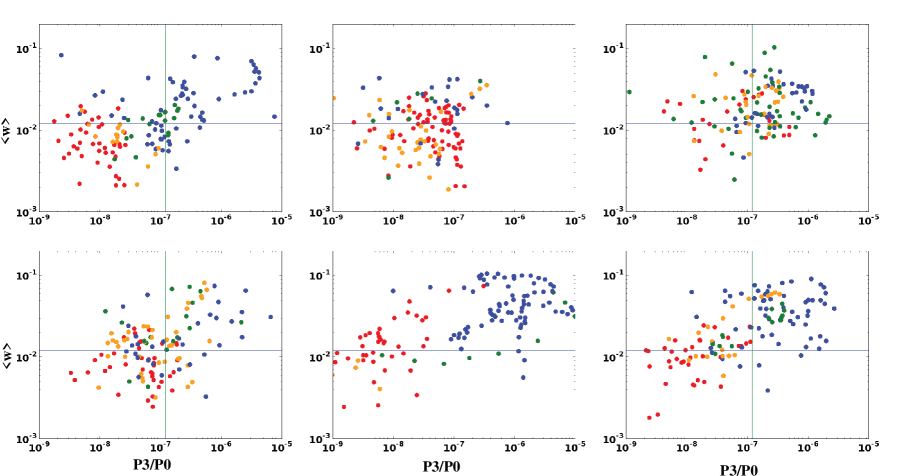
Figure 7: The $P_{3}/P_{0}$-$\langle w\rangle$ plane for projections of all time intervals where $M_{200}>10^{14}M_{\odot}$ for the six $z$=0 clusters whose TKE time histories are shown in Figure 2. In this plot, $\langle w\rangle$ is the centroid shift with the core excluded. Lines indicate the fiducial cut lines in $P_{3}/P_{0}$ and $\langle w\rangle$ in Cassano et al. (2010). Points are colored to indicate the relative level of turbulence kinetic energy for each time interval. Red indicates intervals where $k<2k_{min}$, where $k_{min}$ is the minimum value of the TKE over the full time range for a given cluster. Yellow indicates $2k_{min}<k<3k_{min}$, green is $3k_{min}<k<4k_{min}$, and blue is for $k>4k_{min}$.

Figures 8 and 9 show the correlation between the turbulence kinetic energy and the location of the cluster’s projected structure measures. These plots show the fraction of time for each cluster that it spends in an elevated TKE state (either twice or three times the minimum of $k$) versus the time spent in the upper right quadrant or lower left quadrant of the $P_{3}/P_{0}$-$\langle w\rangle$ plane. It is clear that these two measures are correlated, though there is significant scatter. To first order, the clusters that spend more time in the elevated $k$ states spend more time with disturbed structure measures. It is also evident that the converse is true, those that spend more time in elevated $k$ states spend less time in the lower left of the structure plane. It is also obvious from these Figures that the range of values for fractions of time spent in various regimes are large. Some clusters spend a large fraction of time with elevated TKE and disturbed morphology, while others spend almost no time in these states. It is important to note that clusters do not follow some standard evolutionary path, where they each spend a typical fraction of time in elevated TKE states, but that each evolutionary track is unique. There is a wide range of evolutionary histories, even in a sample this small.

Table 1 shows, for the whole sample of clusters and time outputs, the fraction of time that the structure measures lie in both the relevant quadrants of the $P_{3}/P_{0}$-$\langle w\rangle$ plane and in elevated TKE states. The table shows clearly that clusters that have disturbed structure measures are much more likely to have elevated TKE. While this correlation is not perfect, if a cluster has disturbed structure measures, it has a 92% chance of having its TKE at least double the minimum over the interval in question. Likewise, only a small fraction of clusters with structure measures indicating that they are relaxed have very elevated TKE. Though relaxed structure measures can not perfectly predict low TKE, a number of factors contribute to this problem. First, the use of $k_{min}$ as the base level for TKE almost certainly adds scatter to the correlation. Also, as we have shown in earlier sections, there are moments (particularly at merger core passage) where structure measures look relaxed, yet the TKE is elevated.

In Cassano et al. (2010), a strong case is made that there is a real correlation between incidence of radio halos and location in the planes described by combinations of the concentration parameter, $\langle w\rangle$ and $P_{3}/P_{0}$. The correlation found found here between cluster structure and elevated TKE lends credence to the claims of Cassano et al. (2010) and others that turbulence could indeed be the energy source for the CRs that create the radio halo emission.

Table 1: Fraction of Time with Elevated TKE for Location in Structure Plane

$P_{3}/P_{0}$-$\langle w\rangle$ Quad	2x TKE	3x TKE	4x TKE
Upper Right	0.92	0.77	0.58
Lower Left	0.44	0.19	0.13

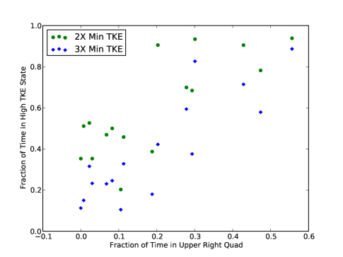
Figure 8: Correlation of the time spent by our simulated clusters in elevated turbulence kinetic energy states with the fraction of time spent in the upper right (disturbed) quadrant of the $P_{3}/P_{0}$-$\langle w\rangle$ plane (as defined by Cassano et al. (2010). Green points represent a value of $k>2k_{min}$, blue indicates $k>3k_{min}$. Note that some clusters spend almost the entire interval we studied in a high TKE state, while others spend almost no time at all in that state.

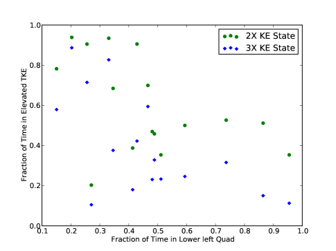
Figure 9: Correlation of the time spent by our simulated clusters in elevated turbulence kinetic energy states with the amount of time spent in the lower left (relaxed) quadrant of the $P_{3}/P_{0}$-$\langle w\rangle$ plane (as defined by Cassano et al. (2010). Green points represent a value of $k>2k_{min}$, blue indicates $k>3k_{min}$.

3.3.2 X-ray Luminosity versus Turbulence Kinetic Energy

Under the assumption that turbulent bulk motions provide the energy source for the CR electrons radiating as radio halos, we plot the total (not specific) turbulence kinetic energy $K_{t}=M_{gas}k$ against the synthetic X-ray luminosity of our simulated clusters in Figure 10. The X-ray luminosity is extracted from the projected maps used for the structure measures, and the turbulence kinetic energy is integrated in each cluster volume (radius of 500kpc). The relation is shown in Figure 10 for a randomly selected 10% of the timesteps in each cluster history (to avoid the appearance of evolutionary tracks). We can not expect identical behavior to the $L_{x}-P_{1.4GHz}$ relation for observed clusters due to the complicating factors of the magnetic field strength and distribution, and the aging of the accelerated particles. However, it is interesting to check whether the “switch” for on/off states of radio halos results directly from a quick transition in turbulence state. Previous work (e.g., Paul et al., 2011) suggests that turbulent pressure is long-lived in the ICM after mergers. Our relation shows no obvious evidence for bimodality in the relation between X-ray luminosity and turbulence kinetic energy. Indeed, our result suggests that the transition from turbulent to relaxed is gradual, as indicated by our earlier time histories. Our analysis shows that there is an order of magnitude spread in the value of $K_{t}$ for a given X-ray luminosity. This result is consistent with Rudnick & Lemmerman (2009), which indicates that the value of $P_{1.4}$ can take on a range of values for a given $L_{x}$, under some upper envelope. It is possible that once a large population of radio halos can be detected at longer wavelengths (given their steep radio spectra) any clear bimodality in the $L_{x}$-$P_{R}$ relations will be washed out. Also, though the $L_{x}-K_{t}$ relation presented here is not bimodal, there are other relevant physical effects on the radio emission (magnetic field strength and variation, presence and spectrum of a pre-existing electron population) which are not included here that could induce strong effects on the resulting $L_{x}-P_{R}$ ratio. For example, Brunetti et al. (2009) suggest that as the turbulent kinetic energy decays following a merger, the the suppression of the synchrotron emissivity in a fixed radio band will be strong. This also suggests that a factor of two difference in the value of $k$ will lead to a factor of 10 suppression in the synchrotron luminosity at 1.4 GHz. In that case, a continuous distribution in $K_{t}$ for a given $L_{x}$, as appears in our figure, will still show a sharp boundary, leading to the observed bimodality.

Figure 10: Synthetic 0.3-8.0 keV X-ray luminosity versus the total turbulence kinetic energy ($M_{gas}k$) for a randomly selected 10% of the time outputs for all clusters and their progenitors in our sample. $L_{x}$ is determined from the projected mock images, $K_{t}$ is extracted from the three-dimensional simulation data.

4 DISTRIBUTION AND DURATION OF TURBULENCE IN SIMULATED CLUSTERS

If in fact turbulent re-acceleration is responsible for generating the relativistic electrons powering radio halos, then the evolution of the TKE in our simulated clusters can tell us about the possible lifetime of radio halos and the frequency with which clusters are expected to host radio halos. In this section, we examine the typical duration of episodes of elevated turbulence (i.e. the merger relaxation time) and the fraction of clusters at a given time that are in elevated TKE states.

4.1 Lifetime of Merging Events

We have run an analysis to determine the typical timescale for clusters in our sample to be in elevated TKE states. We take every cluster’s time history and identify all time intervals over which the TKE is continuously elevated to at least 2$k_{min}$. The histogram of those intervals is shown in Figure 11. The median length of time that a cluster spends in a continuously elevated TKE state by this definition is $t_{ele}=1.13$ Gyr. If we redefine the intervals by elevation to 3$k_{min}$ or above, then $t_{ele}=0.77$ Gyr. For $k>4k_{min}$, $t_{ele}=0.77$ Gyr. While it may not be obvious why the median interval for the highest two $k$ bins should be the same, the rough shape of the distribution is preserved at these ranges, though the normalization has declined. So it is safe to say from our sample that the median time interval over which the TKE is elevated inside r =500 kpc is around 1 Gyr, or slightly less depending on the threshold used. However, Figure 11 also shows a tail to very long intervals of elevated TKE with some clusters having time periods of 5 or more Gyrs with continuously elevated TKE. This result again shows the diversity of cluster histories: in the turbulent re-acceleration model some clusters would be expected to host radio halos over most of their lifetime while other clusters never would.

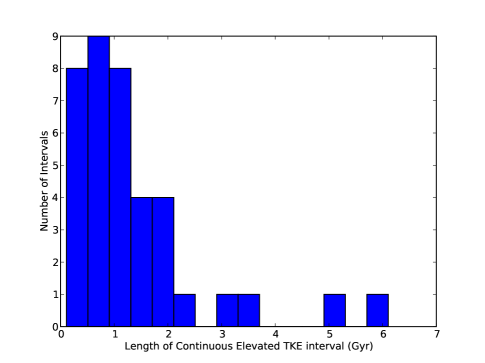
Figure 11: Histogram of all continuous time intervals for clusters in our sample where the turbulence kinetic energy inside r=500 $kpc$ is elevated to $k>2k_{min}$. The median interval length is 1.12 $Gyr$.

Continuous time intervals for elevated structure measures show a different result. The median value for intervals of $P_{3}/P_{0}$ elevated above the Cassano et al. (2010) limit is much shorter than the elevated $k$ intervals at $t_{ele}=0.33Gyr$. For the centroid shift we see a similar result of $t_{ele}=0.39Gyr$. This result is not particularly surprising given the time histories shown in Figures 4, 5 and 6. The values of the structure measures are more highly variable over short time scales than the value of $k$, and can show strong variations at core passage for instance. If we identify by eye time periods with low structure measures associated to core passage events and interpolate over them, a longer typical timescale for elevated structure measure of around $0.5Gyr$ is found, though this procedure is subjective.

4.2 Fraction of Clusters with Elevated Turbulence Kinetic Energy

If the energy source for giant radio halos is turbulent re-acceleration, an interesting measure is the fraction of objects with elevated turbulence kinetic energy. In Figure 12, we show the fraction of massive clusters (M$\geq 5\times 10^{14}M_{\odot})$ as a function of redshift that have $k$ elevated by an integer factor above the minimum over their history. The fraction is a noisy, but gradually declining function of time depending on what threshold of $k$ is used. For $k>3k_{min}$ as shown in Figure 12, the fraction of clusters with elevated TKE at high redshift ($z>0.4$) is noisy, but high (50-100%), and declines to roughly 20% at $z=0$. The trend for values of $k>2k_{min}$ and $k>4k_{min}$ is similar, but the normalization changes. For $k>2k_{min}$ the typical fraction of clusters declines from 60-100% at the higher redshifts to 35-50% at $z$=0. For $k>4k_{min}$ the fraction is 50-100% at high $z$, with a drop to around 8% at $z$=0. Our results imply that the fraction of massive clusters that are energetically favorable for producing CRs through turbulent re-acceleration is declining with redshift.

Observational searches find a fraction of roughly 30% of clusters at moderate redshifts ($0.2<z<0.4$) hosting radio halos (Venturi et al., 2008). This result will obviously depend on the survey depth and should also depend strongly on the frequency of observation, as steep spectrum radio sources are much brighter at longer wavelengths. In addition, we should point out that radiative losses to relativistic particles due to inverse Compton (IC) interactions with the CMB scale as (1+$z)^{4}$, strongly limiting the possibility of radio halos at the higher redshifts (Cassano & Brunetti, 2005; Cassano et al., 2006). Given the uncertainty in the energetic threshold for TKE to produce a radio halo, our range for the fraction of clusters with elevated TKE in the redshift range of most observed radio halos ($0.2<z<0.4$) of 20-50% is broadly consistent with the observed ratio.

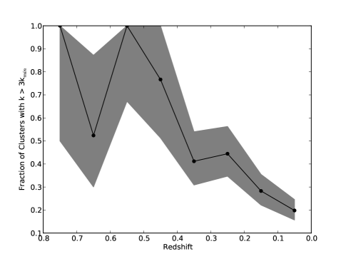
Figure 12: The fraction of simulated massive ($M>5\times 10^{14}M_{\odot}$) clusters as $f(z)$ that have $k>3k_{min}$. Shaded region shows Poisson error bars due to the finite sample of simulated clusters at each redshift.

5 DISCUSSION

Observations show a connection between the detection of diffuse, large-scale radio halo emission and the presence of merging activity in clusters (e.g. Buote, 2001; Cassano et al., 2010). In particular, these studies show a correlation between observed X-ray cluster structure, quantified based on the centroid shift and the power ratios, and the presence of radio halo emission. While the origin of radio halos is still a matter of debate, it has been suggested that merger generated turbulence could accelerate a pre-existing relativistic electron population (from supernovae, AGN, previous merger/shock activity) to energies sufficient to produce the radio emission.

In this paper, we study the evolution with time of massive clusters formed within a numerical hydrodynamic, cosmological simulation and investigate whether a subset of the X-ray and radio observational evidence from clusters is consistent with the turbulent re-acceleration model for radio halos. In particular, we track the evolution of random bulk ICM motions, the kinetic energy of which is dissipated through shocks and the turbulent cascade. We study the relationship between turbulence kinetic energy and X-ray structure measures, how these evolve during mergers, and whether the level of turbulence in simulated clusters with radio halo-like cluster structures supports the turbulent re-acceleration model.

We show that the distribution of the X-ray structure measures (centroid shift $w$ and third order power ratio $P_{3}/P_{0}$) used by Cassano et al. (2010) to separate radio halo and non-radio halo clusters are reproduced fairly well in our simulated cluster sample and that a similar fraction of simulated clusters have ”disturbed” X-ray structures compared to observations. We also find that clusters in the disturbed regimes of the structure plane are highly likely to have elevated turbulence kinetic energy (at the scales we resolve). For some clusters, we have shown this graphically (Figure 7). Quantitatively, clusters with structure measures in the “disturbed” part of the structure plane have a 92% chance of having an elevated $k$ at least two times above the minimum over the cluster lifetime. Though individually, there is a significant amount of variation in the structure measures for a given value of $k$, as a group they correlate strongly. Cassano et al. (2010) suggest that the fact that radio halo clusters are more disturbed in terms of their structure measures results from a difference in the amount of turbulence in disturbed versus relaxed clusters and that turbulent re-acceleration of CR electrons is the source of radio halos in galaxy clusters. The strong correlation between cluster structure and elevated turbulence in simulated clusters supports this theory.

The value of the turbulence kinetic energy $k$ undergoes large variations during mergers of factors of a few to several. Mergers are typically well-defined in $k(z)$, with $k$ smoothly increasing and then decreasing through the merger, though additional mergers can (not infrequently) occur before the system can fully relax. The time evolution of the structure measures during mergers are not as well defined and are a strong function of merger phase. Both $P_{3}/P_{0}$ and $\langle w\rangle$ are noisier than $k$ as a function of time in our simulated clusters. A classic example in many of our simulated clusters is the sharp reduction in the values of the structure measures as a merger proceeds through the core passage of a subcluster. Though the turbulence kinetic energy is high at this stage, the object could be called “relaxed” using the structure measures and significant substructure is not visible in the X-ray image. The result of this difference is that the time scales for continuously elevated $k$ are of order 2-3 times longer than those for elevated structure measures. The median interval for enhanced $k$ to twice the minimum for a given cluster is approximately $\tau$=1 Gyr. For $P_{3}/P_{0}$ and $\langle w\rangle$, this number is closer to $\tau$= 0.33 Gyr. For these reasons, translating from the observed structure measures to the dynamical state, or more specifically to the energetics of the bulk motion of the gas, has significant scatter for individual clusters. However, statistically these properties correlate well.

Though prior studies suggest turbulent kinetic energy is very long-lived in clusters (e.g., Paul et al., 2011), we show that $k$ drops significantly in cluster volumes over much shorter timescales ($\sim 0.5$ Gyr). However, these results may be consistent, given that the Paul et al. (2011) result uses a different criterion (turbulent pressure $>5$% of the total pressure) than we do for elevated turbulence. The relatively quick drop in TKE, coupled to short synchrotron cooling times, may account for the sharp difference in X-ray structure for RH versus non-RH clusters.

An interesting result of this work is that we find that many clusters spend a large fraction ($\sim$80+%) of their time in disturbed states, while others spend very little time ($\sim$10%) in such states. Thus, it may be the case that some galaxy clusters are rarely, if ever radio halo clusters during their lifetime, while others almost always host radio halos. While the typical timescale for the turbulence kinetic energy to be elevated is $\sim 1$ Gyr, these periods can be as long as 5 or more Gyrs in cluster which experience complex or repeated mergers.

Finally, we find no obvious evidence for bimodality of the $L_{x}$-$K$ relation (where $K$ could be a proxy for radio power) in our simulated sample of clusters. However, this is not necessarily surprising given that there are a number of reasons why such a gap may exist in the observed $L_{x}$-$P_{1.4}$ relation that are unrelated to the dynamical state of the gas. For example, we have not modeled magnetic field variations, and the turbulent re-acceleration mechanism requires a pre-existing population of CRs on which to operate, both of which may vary from cluster to cluster. Brunetti et al. (2009) have shown that the relationship between the kinetic energy in turbulence and the fixed band radio luminosity is not linear. Their work suggests that a relatively small drop in TKE results in a large change in the synchrotron luminosity, which could easily account for the observed bimodality, yet still be consistent with our result here. To fully understand this issue, it is necessary to follow the magnetic fields and CR particles explicitly in the simulation to see the true evolution of the radio emission. A full treatment of simulating a large sample of galaxy clusters and their radio emission must handle the injection of CRs into the ICM from reasonable sources like AGN, SNe, and large-scale accretion shocks. This work we defer to upcoming simulations using a new MHD+CR code.

References

- Bagchi et al. (2006) Bagchi, J., Durret, F., Neto, G. B. L., & Paul, S. 2006, Science, 314, 791
- Braginskii (1958) Braginskii, S. I. 1958, Soviet Journal of Experimental and Theoretical Physics, 6, 494
- Brunetti (2004) Brunetti, G. 2004, Journal of Korean Astronomical Society, 37, 493
- Brunetti et al. (2009) Brunetti, G., Cassano, R., Dolag, K., & Setti, G. 2009, A&A, 507, 661
- Brunetti et al. (2008) Brunetti, G., Giacintucci, S., Cassano, R., Lane, W., Dallacasa, D., Venturi, T., Kassim, N. E., Setti, G., Cotton, W. D., & Markevitch, M. 2008, Nature, 455, 944
- Brunetti & Lazarian (2011) Brunetti, G. & Lazarian, A. 2011, MNRAS, 410, 127
- Brunetti et al. (2001) Brunetti, G., Setti, G., Feretti, L., & Giovannini, G. 2001, MNRAS, 320, 365
- Bryan & Norman (1997a) Bryan, G. & Norman, M. 1997a, 12th Kingston Meeting on Theoretical Astrophysics, proceedings of meeting held in Halifax; Nova Scotia; Canada October 17-19; 1996 (ASP Conference Series # 123), ed. D. Clarke. & M. Fall
- Bryan & Norman (1997b) —. 1997b, Workshop on Structured Adaptive Mesh Refinement Grid Methods, ed. N. Chrisochoides (IMA Volumes in Mathematics No. 117)
- Buote (2001) Buote, D. A. 2001, ApJL, 553, L15
- Buote & Tsai (1995) Buote, D. A. & Tsai, J. C. 1995, ApJ, 452, 522
- Carilli & Taylor (2002) Carilli, C. L. & Taylor, G. B. 2002, ARA&A, 40, 319
- Cassano (2009) Cassano, R. 2009, in Astronomical Society of the Pacific Conference Series, Vol. 407, The Low-Frequency Radio Universe, ed. D. J. Saikia, D. A. Green, Y. Gupta, & T. Venturi, 223–+
- Cassano & Brunetti (2005) Cassano, R. & Brunetti, G. 2005, MNRAS, 357, 1313
- Cassano et al. (2006) Cassano, R., Brunetti, G., & Setti, G. 2006, MNRAS, 369, 1577
- Cassano et al. (2010) Cassano, R., Ettori, S., Giacintucci, S., Brunetti, G., Markevitch, M., Venturi, T., & Gitti, M. 2010, ApJL, 721, L82
- Choudhuri (1998) Choudhuri, A. R. 1998, The physics of fluids and plasmas : an introduction for astrophysicists /, ed. Choudhuri, A. R.
- Clarke & Ensslin (2006) Clarke, T. E. & Ensslin, T. A. 2006, AJ, 131, 2900
- Eisenstein & Hu (1999) Eisenstein, D. J. & Hu, W. 1999, ApJ, 511, 5
- Eisenstein & Hut (1998) Eisenstein, D. J. & Hut, P. 1998, ApJ, 498, 137
- Feretti et al. (2001) Feretti, L., Fusco-Femiano, R., Giovannini, G., & Govoni, F. 2001, A&A, 373, 106
- Ferland et al. (1998) Ferland, G. J., Korista, K. T., Verner, D. A., Ferguson, J. W., Kingdon, J. B., & Verner, E. M. 1998, PASP, 110, 761
- Ferrari et al. (2008) Ferrari, C., Govoni, F., Schindler, S., Bykov, A. M., & Rephaeli, Y. 2008, SSR, 134, 93
- Giacintucci et al. (2009) Giacintucci, S., Venturi, T., Cassano, R., Dallacasa, D., & Brunetti, G. 2009, ApJL, 704, L54
- Govoni & Feretti (2004) Govoni, F. & Feretti, L. 2004, International Journal of Modern Physics D, 13, 1549
- Govoni et al. (2004) Govoni, F., Markevitch, M., Vikhlinin, A., van Speybroeck, L., Feretti, L., & Giovannini, G. 2004, ApJ, 605, 695
- Hallman et al. (2010) Hallman, E. J., Skillman, S. W., Jeltema, T. E., Smith, B. D., O’Shea, B. W., Burns, J. O., & Norman, M. L. 2010, ApJ, 725, 1053
- Hardcastle et al. (2003) Hardcastle, M. J., Worrall, D. M., Kraft, R. P., Forman, W. R., Jones, C., & Murray, S. S. 2003, ApJ, 593, 169
- Jeltema et al. (2005) Jeltema, T. E., Canizares, C. R., Bautz, M. W., & Buote, D. A. 2005, ApJ, 624, 606
- Jeltema et al. (2008) Jeltema, T. E., Hallman, E. J., Burns, J. O., & Motl, P. M. 2008, ApJ, 681, 167
- Jeltema & Profumo (2011) Jeltema, T. E. & Profumo, S. 2011, The Astrophysical Journal, 728, 53
- Kassim et al. (2001) Kassim, N. E., Clarke, T. E., Enßlin, T. A., Cohen, A. S., & Neumann, D. M. 2001, ApJ, 559, 785
- Keshet (2010) Keshet, U. 2010, ArXiv e-prints
- Keshet & Loeb (2010) Keshet, U. & Loeb, A. 2010, ApJ, 722, 737
- Kushnir et al. (2009) Kushnir, D., Katz, B., & Waxman, E. 2009, JCAP, 9, 24
- Liang et al. (2000) Liang, H., Hunstead, R. W., Birkinshaw, M., & Andreani, P. 2000, ApJ, 544, 686
- Macario et al. (2010) Macario, G., Venturi, T., Brunetti, G., Dallacasa, D., Giacintucci, S., Cassano, R., Bardelli, S., & Athreya, R. 2010, A&A, 517, A43+
- Norman & Bryan (1999) Norman, M. & Bryan, G. 1999, Numerical Astrophysics : Proceedings of the International Conference on Numerical Astrophysics 1998 (NAP98), held at the National Olympic Memorial Youth Center, Tokyo, Japan, March 10-13, 1998., ed. K. T. S. M. Miyama & T. Hanawa (Kluwer Academic)
- Nulsen et al. (2005) Nulsen, P. E. J., McNamara, B. R., Wise, M. W., & David, L. P. 2005, ApJ, 628, 629
- O’Shea et al. (2004) O’Shea, B., Bryan, G., Bordner, J., Norman, M., Abel, T., & Harkness, R. amd Kritsuk, A. 2004, Adaptive Mesh Refinement - Theory and Applications, ed. T. Plewa, T. Linde, & G. Weirs (Springer-Verlag)
- O’Shea et al. (2005) O’Shea, B. W., Nagamine, K., Springel, V., Hernquist, L., & Norman, M. L. 2005, ApJS, 160, 1
- Paul et al. (2011) Paul, S., Iapichino, L., Miniati, F., Bagchi, J., & Mannheim, K. 2011, ApJ, 726, 17
- Petrosian (2001) Petrosian, V. 2001, ApJ, 557, 560
- Pfrommer et al. (2008) Pfrommer, C., Enßlin, T. A., & Springel, V. 2008, MNRAS, 385, 1211
- Roettiger et al. (1999) Roettiger, K., Burns, J. O., & Stone, J. M. 1999, ApJ, 518, 603
- Rudnick & Lemmerman (2009) Rudnick, L. & Lemmerman, J. A. 2009, ApJ, 697, 1341
- Sarazin (2004) Sarazin, C. L. 2004, Journal of Korean Astronomical Society, 37, 433
- Skillman et al. (2010) Skillman, S. W., Hallman, E. J., O’Shea, B. W., Burns, J. O., Smith, B. D., & Turk, M. J. 2010, ArXiv 1006.3559
- Spitzer (1962) Spitzer, L. 1962, Physics of Fully Ionized Gases, ed. Spitzer, L.
- Turk et al. (2011) Turk, M. J., Smith, B. D., Oishi, J. S., Skory, S., Skillman, S. W., Abel, T., & Norman, M. L. 2011, ApJS, 192, 9
- van Weeren et al. (2010) van Weeren, R. J., Röttgering, H. J. A., Brüggen, M., & Hoeft, M. 2010, Science, 330, 347
- Venturi et al. (2008) Venturi, T., Giacintucci, S., Dallacasa, D., Cassano, R., Brunetti, G., Bardelli, S., & Setti, G. 2008, A&A, 484, 327