The ultimate limits of precision pulsar timing

Abstract

We demonstrate that the sensitivity of high-precision pulsar timing experiments will be ultimately limited by the broadband intensity modulation that is intrinsic to the pulsar’s stochastic radio signal. That is, as the peak flux of the pulsar approaches that of the system equivalent flux density, neither greater antenna gain nor increased instrumental bandwidth will improve timing precision. These conclusions proceed from an analysis of the covariance matrix used to characterise residual pulse profile fluctuations following the template matching procedure for arrival time estimation. We perform such an analysis on 25 hours of high-precision timing observations of the closest and brightest millisecond pulsar, PSR J0437$-$4715. In these data, the standard deviation of the post-fit arrival time residuals is approximately four times greater than that predicted by considering the system equivalent flux density, mean pulsar flux and the effective width of the pulsed emission. We develop a technique based on principal component analysis to mitigate the effects of shape variations on arrival time estimation and demonstrate its validity using a number of illustrative simulations. When applied to our observations, the method reduces arrival time residual noise by approximately 20%. We conclude that, owing primarily to the intrinsic variability of the radio emission from PSR J0437$-$4715 at 20 cm, timing precision in this observing band better than 30 - 40 ns in one hour is highly unlikely, regardless of future improvements in antenna gain or instrumental bandwidth. We describe the intrinsic variability of the pulsar signal as stochastic wideband impulse modulated self-noise (SWIMS) and argue that SWIMS will likely limit the timing precision of every millisecond pulsar currently observed by Pulsar Timing Array projects as larger and more sensitive antennas are built in the coming decades.

1 Introduction

The most fundamental property of radio pulsars is their periodic series of radio pulses that enable their discovery and a myriad of timing applications. A sub-class of pulsars, known as the millisecond and recycled pulsars, have spin periods between 1.4 and a few tens of ms and typical spin-down rates of $\dot{P}\sim 10^{-20}$. Their short periods and low braking torques make them especially good clocks, and these pulsars exhibit the highest timing precision (Matsakis et al., 1997). For most of these pulsars a simple model of the pulsar spin-down, astrometric and orbital parameters can be determined, enabling the mean time-of-arrival (ToA) of pulses to be predicted accurately and precisely. These can be used for several applications, such as testing the general theory of relativity (e.g. Taylor & Weisberg, 1982; Kramer et al., 2006b), detecting irregularities in terestrial time standards (Petit & Tavella, 1996; Rodin, 2008; Hobbs et al., 2010) and to attempt the first direct detection of a stochastic background of gravitational waves (see, e.g. Hellings & Downs, 1983; Foster & Backer, 1990; Demorest, 2007; Yardley et al., 2010; van Haasteren et al., 2011). The wealth of information already derived from the precision timing of millisecond radio pulsars has led many authors to predict the kind of pulsar timing science possible with the Square Kilometre Array (SKA) by linearly extrapolating current telescope sensitivities to that of the SKA.

The closest and brightest millisecond pulsar known, PSR J0437$-$4715 (Johnston et al., 1993) has been studied by numerous authors with steadily improving instrumentation. Sandhu et al. (1997) observed the pulsar using an autocorrelation spectrometer with 128 MHz of bandwidth, and could model pulse arrival times over two years with a post-fit residual (the difference between observed and predicted arrival times after fitting for the pulsar spin, astrometric and binary parameters, etc.; Taylor, 1992) standard deviation of $500$ ns. Noting that the formal uncertainty of arrival time estimates was typically around 50 ns, the authors concluded that their results were limited by polarimetric calibration errors. Britton (2000) first proposed the use of the Stokes invariant interval to mitigate the problems caused by polarisation calibration. This was later implemented by van Straten et al. (2001), who used a combination of 16 MHz and 20 MHz baseband recording systems, typical integrations of 1 hour duration, and coherent dedispersion to obtain a root-mean-square (rms) timing residual of 130 ns over 3.4 yr. Using new and improved calibration methods developed by van Straten (2004, 2006) and a new baseband recording and processing system (CPSR2; Bailes, 2003; Hotan, 2006) with 128 MHz of bandwidth, Verbiest et al. (2008) achieved $199$ ns over 10 years.

None of the above studies achieve the timing precision predicted by the formal uncertainty in arrival time estimates. When observing PSR J0437$-$4715 in the 20 cm band at the Parkes $64$m observatory, the expected rms timing residual from a 256 MHz band with $21$ K system temperature is about 10 and 80 ns in one hour and one minute of integration, respectively. These uncertainties are derived from the template-matching method used for pulsar timing, in which each observation of the average pulse profile $O(t)$ is modelled as a scaled (A) and offset (B) template $S(t)$, rotated by some phase shift $\phi$, with additional white noise $N(t)$ (Taylor, 1992; Bailes, 2010).

$$O(t)=AS(t-\phi)+B+N(t).$$ (1)

It is generally assumed that the summation of many hundreds or thousands of pulses leads to a stable pulse profile that is characteristic of the pulsar (Helfand et al., 1975). Consideration of only additional white noise, $N(t)$, in the above equation is equivalent to assuming that the system equivalent flux density is the only significant source of noise. However for bright sources and/or high gain antenna, this assumption is no longer tenable in at least two circumstances. Firstly, when the flux density of the pulsar approaches the system equivalent flux density (SEFD) of the receiver additional noise proportional to the pulsar’s flux density becomes significant (e.g. Kulkarni, 1989; Gwinn, 2001, 2004, 2006; van Straten, 2009; Gwinn & Johnson, 2011; Gwinn et al., 2011). Secondly, it is known that each single pulse can have very different morphology and can occur at different pulse phase (Drake & Craft, 1968; Helfand et al., 1975; Jenet et al., 1998). Even after integrating over many pulse periods, this subpulse modulation can introduce detectable fluctuations in the average profile shape and thereby contribute additional noise to timing data. We discuss the noise balance in more detail in §2, and argue that these two contributions should be considered together as they are related and are described by the same statistical model.

We note that the presence and importance of pulse profile variability have been discussed in many different contexts. Some “classical” pulsars have been observed to change between two or more stable profiles – a phenomenon known as mode changing – on time-scales of minutes to hours (e.g. Backer, 1970; Bartel et al., 1982). On longer time scales, pulsars have been discovered whose emission completely switches off for many days, weeks or even months (e.g. Durdin et al., 1979; Kramer et al., 2006a). Recently, Lyne et al. (2010) have shown that the pulse profiles for many pulsars switch between two unique states on time-scales of months to years. Karastergiou et al. (2011) recently detected a transient component in PSR J0738$-$4042, varying on time-scale of years or decades.

The connection between the pulse shape changes and timing noise was made soon after the discovery of timing noise in the pulsar observations by Boynton et al. (1972). They studied optical timing observations of the Crab pulsar and discovered a noise component in the timing residuals which was well modelled as a random walk in the pulsar spin frequency. The authors also considered a random walk in the pulse phase and spin frequency derivative, but found no evidence of such noise in their data. This analysis was extended in a series of papers (Groth, 1975a, b, c). The author presented an analysis method suitable for studies of data with inherent timing noise. This improved methodology led to the conclusion that noise in the Crab pulsar timing is dominated by a random walk in the spin frequency but a random walk in pulsar phase might also be present. In the meantime, Manchester & Taylor (1974) described timing noise for two slow pulsars from radio observations. A few years later, another series of papers (Helfand et al., 1980; Cordes, 1980; Cordes & Helfand, 1980) presented statistics of timing noise for 37 bright pulsars and concluded that it is a ubiquitous phenomenon. These authors presented a careful analytical description of random walks in pulsar phase, spin frequency and its derivative and the uncertainties in the estimation of their parameters. The last paper in the series pointed out that the random walk in the pulsar phase can be due to the random pulse shape changes but concluded that it was unlikely to be the dominant source of timing noise in the available data. A different dataset was analysed in a similar manner by Cordes & Downs (1985) who stated that either excessive jitter or pulse shape changes are important for a significant fraction of their sample. They also pointed out that the pulse shape changes are likely to be universal but their importance varies from object to object. Later, Cordes (1993) detected pulse shape variability in 11 out of 14 studied objects. These variations were consistent with being caused by summation of a finite number of pulses. A year later Kaspi et al. (1994) studied two millisecond radio pulsars and discovered timing noise in one of them. The general continuity of properties between classical and millisecond pulsars suggests that pulse shape changes may be common in millisecond pulsars as well.

The profile variability of millisecond pulsars (MSPs) has been studied in relatively few cases. The single pulses from PSR J1939$+$2134 show no subpulse structure over selected ranges of pulse longitude (Jenet et al., 2001) but emit giant pulses as much as 300 times brighter than the average pulse, that are narrower and systematically delayed with respect to the main and interpulse components (Cognard et al., 1996; Kinkhabwala & Thorsett, 2000). Several other groups have argued that MSPs exhibit profile shape changes. Some are associated with different viewing geometries or with gravitational spin-orbit coupling; e.g. PSR B1913$+$16 (Weisberg et al., 1989; Kramer, 1998) and PSR B1534$+$12 (Arzoumanian, 1995; Stairs et al., 2000). Backer & Sallmen (1997) claimed erratic emission modes from PSR B1821$-$24 but at only one observing frequency. In another work, Kramer et al. (1999) studied PSRs J1022$+$1001 and J1730$-$2304. In both cases, they detected profile variations over time-scales of the order of $10$ to $15$ minutes; however the data quality for the latter did not allow a rigourous statistical analysis. On the other hand, Hotan et al. (2004a) detected no significant variations in the pulse profile of PSR J1022$+$1001 and demonstrated that the reported profile shape variations could be explained by polarisation calibration errors.

Small profile changes in PSR J0437$-$4715 were described by Vivekanand et al. (1998) using observations performed at a very low frequency with only a single polarisation. This result was contested by Sandhu et al. (1997), who argued that calibration errors were the origin. Vivekanand (2001) later argued that the variations are intrinsic to the pulsar and correlated with spiky emission in the varying component. Variations in the central region of the profile were also reported by Navarro et al. (1997) with $24$ minute integrations at $428$ MHz but they were not investigated in detail. Liu et al. (2011) developed a sharpness statistic but found it insesitive to profile changes in PSR J0437$-$4715.

As described in more detail in §2, this work focuses on the stochastic fluctuations in total intensity that arise from the subpulse structure observed in single pulses and their effect on the timing precision attainable for PSR J0437$-$4715. In §3 our observations are described along with the applied data processing followed by results of timing our observations. In §4 we describe a statistical method useful for detecting profile shape variations, then apply it to simulated data as a demonstration of how it can be used to correct ToA residuals. The results of the statistical analysis are presented in §5. We summarise our findings and discuss their consequences in §6, which also contains a discussion of other possible problems that prevent us from reaching the theoretical timing accuracy. Finally we draw our conclusions in §7.

2 Stochastic Wideband Impulse Modulated Self-Noise

The noise $N(t)$ in equation 1 is normally assumed to be dominated by the white radiometer noise. In practice, for bright sources and/or high gain antennas, two additional effects may contribute significantly. In this section we discuss the noise balance for pulsars and demonstrate that the different contributions are well described by a single statistical model.

Firstly, the noise balance has to include the source itself when the flux density of the pulsar approaches the SEFD. This noise is intrinsic to the source and is accordingly called “self-noise”. In the case of PSR J0437$-$4715, the mean flux at the peak of the pulse profile is of the order of 5 Jy; this contributes only $\sim 2\%$ to the standard deviation of the total intensity, which is dominated by the SEFD $\sim 27$ Jy of the 20 cm multibeam receiver (Manchester et al., 2001) commonly used for pulsar timing observations at Parkes. Any source that can be described as noise (e.g. thermal emission) will contribute to the variance of the observed total intensity of the source. When the signal-to-noise ratio ($S/N$) is low, this contribution is negligible. We note that throughout the paper we use $S/N$ values calculated using the noise measured in the off-pulse baseline.

Secondly, dramatic subpulse amplitude modulation is a ubiquitous feature of radio pulsar emission (Rickett, 1975) that spans orders of magnitude in intensity and duration and is a broadband phenomenon (e.g. Staelin & Reifenstein, 1968; Taylor et al., 1975; Manchester et al., 1975; Hankins et al., 1993; Hankins & Eilek, 2007; Wang et al., 2007). The subpulse emission from PSR J0437$-$4715 is well studied; Jenet et al. (1998) observe an exponential distribution of peak subpulse intensities with a mean flux density of 16.6 Jy, which is comparable to the SEFD. More importantly, the mean subpulse width of $65$ $\mu$s (Jenet et al., 1998) is about an order of magnitude larger than the interval required to sample the mean pulse profile of PSR J0437$-$4715. Consequently, subpulse intensity fluctuations introduce detectable variations in the average pulse profile. Given the stochastic nature of subpulse structure, these fluctuations in mean pulse profile shape can be expected to introduce significant additional noise in derived arrival time estimates.

In one minute, PSR J0437$-$4715 turns $\sim 10^{4}$ times and emits at least $\sim 2\times 10^{3}$ subpulses (Jenet et al., 1998). After integrating over such a large number of emission events, it is no longer practical to consider the impact of an individual subpulse. Rather, it becomes necessary to describe the effects of subpulse modulation in purely statistical terms using the fourth moments of the electric field (Rickett, 1975). From this perspective, the subpulse modulation phenomenon is a noise process that contributes to the autocorrelation of the total intensity (Rickett, 1975). For a given source flux density, amplitude modulation increases the variance of the total intensity and, depending on the time-scale of the modulations and the sampling interval of the instrument, introduces power at non-zero delays in the autocorrelation of the total intensity.

Measured statistical distributions of subpulse intensities vary between sources and as a function of pulse longitude (e.g. power law, log normal, etc.; for an excellent review, see Cairns, 2004). Regardless of the original distribution, after a large number of pulses have been integrated, the central limit theorem applies and profile shape variations are well described by a multivariate normal distribution. The covariance matrix that quantifies this distribution contains phase-resolved information about the mean autocorrelation of the total intensity.

To summarise, depending on the pulsar’s flux density, its emission properties and the used instrument, we can distinguish three noise regimes:

1. First regime: The pulsar’s flux density is much smaller than the SEFD of the instrument. This is the classic regime, in which the noise is temporally uncorrelated between the phase bins and homoscedastic (i.e., the variance of noise is the same in each phase bin). In this regime the covariance matrix of the pulse profiles is well approximated by a diagonal matrix with all the elements on the diagonal equal to the variance of SEFD.

2. Second regime: The pulsar’s flux density approaches or exceeds the SEFD of the received used. In this regime the self-noise cannot be neglected. The noise is still temporally uncorrelated between the phase bins, but it is heteroscedastic; that is the variance of the noise is different in each bin and proportional to the sum of squares of the pulsar’s flux density and the SEFD. The covariance matrix of the data is still diagonal, but the non-zero elements are no longer equal. In this regime, the on-pulse noise is no longer measured by the off-pulse noise and using the latter to calculate the $S/N$ can lead to overestimating the achievable timing precision.

3. Third regime: The pulsar is heavily amplitude modulated with the modulated flux approaching or exceeding the SEFD of the instrument. Even though the self-noise contribution may be negligible, the modulated subpulses can approach the SEFD of the receiver, thus contributing significant ‘noise’ to the averaged pulse profile. If the sampling rate is high enough to resolve the subpulse structure, the noise in different phase bins will be heteroscedastic and temporally correlated. The off-diagonal elements of the covariance matrix will be non-zero in this regime. If the subpulses are not resolved, amplitude modulation may still be evident in the variation of the modulation index as a function of pulse phase. The broadband nature of the impulses will also lead to spectral correlation of the noise, which can be detected by measuring the covariance of intensity fluctuations in different frequency channels. Therefore, when analysing only the covariance matrix SWIMS might be confused with self-noise.

In this paper, we investigate the effects of the third regime, which we call stochastic wideband impulse modulated self-noise (SWIMS), on pulse arrival time estimation. This pulsar-intrinsic noise has also been called pulse-phase jitter (or jitter noise), “intermittent emission” (Gwinn et al., 2011) or simply self-noise. We will demonstrate that the timing precision of PSR J0437$-$4715 is currently limited by SWIMS and that its effect on the mean pulse profile is readily detectable.

As a function of integration length $T$, the covariance matrix scales as $T^{-1}$; that is, the effects of SWIMS are reduced by integration, regardless of the dominating source of noise. The fact that the covariance matrix scales as $T^{-1}$ allows us to study the statistics of single pulses with longer integrations. If any pulse-to-pulse correlation were present in data, such as arising from drifting subpulses, nulling, mode changing, scattering or polarisation calibration errors, the scaling of the covariance matrix with integration length would deviate from the above proportionality. We note that the relative contribution of source-intrinsic noise to the covariance matrix will vary as the flux density of the pulsar varies, primarily owing to interstellar scintillation. However, after averaging over many scintillation time scales, the relative contribution of SWIMS compared to the SEFD is constant (Kulkarni, 1989); therefore, the relative importance of SWIMS is independent of integration length. We note that in the first or second regime, noise can be reduced by increasing the bandwidth. However, because the intensity fluctuations are typically correlated over wide bandwidths, the noise due to subpulse modulation is not reduced by increasing the bandwidth and only longer integration times and active mitigation can improve timing precision in the third regime.

Gwinn et al. (2011) recently performed a detailed analysis of impulse-modulated self-noise in the context of interstellar scintillation observations and concluded that self-noise may limit pulsar timing precision. In this paper, we explore the impact of both temporal and spectral correlations of intensity fluctuations on pulsar timing and consider active mitigation of SWIMS.

3 Observations and data processing

Observations of PSR J0437$-$4715 were recorded during one week of February 2010 using the Parkes 64 m radio telescope and the central beam of the 20 cm multibeam receiver (Staveley-Smith et al., 1996). The third generation of the Pulsar Digital Filterbank (PDFB3) digitised the voltage data from two orthogonally polarised 256 MHz bands and formed 1024 frequency channels using a polyphase filterbank. After full polarisation detection (following the definitions described by van Straten et al., 2010), the data were folded at the topocentric period of the pulsar into 1024 phase bins. The mean polarisation profile was output every minute and a total of 25 hours of data were recorded. The multibeam receiver is equipped with a noise diode that is coupled to the receptors and driven with a square wave to inject a pulsed polarised reference signal into the feed horn. This signal was recorded for three minutes before and after every 64 minute observation of the pulsar. These data are archived in, and can be obtained through, the Australia Telescope Online Archive and CSIRO Data Access Portal (Hobbs et al., 2011).

The data are stored in the PSRFITS format and all processing was done with the PSRCHIVE data processing software suite (Hotan et al., 2004b). First we ensured that a recent model for the pulsar spin, astrometric and orbital parameters (Verbiest et al., 2008) was used throughout for our data processing. To remove narrow band radio frequency interference (RFI), median filtering was applied by comparing the total flux in each frequency channel with that of its 49 neighbouring channels. To avoid distortions at the edge of the observing band, we rejected five per cent of the frequency channels on each side of the band. A search for impulsive RFI was performed with the “lawn mower” method. Pulsar observations were calibrated for polarisation as in van Straten (2004). The flux density was calibrated by observing the Hydra A radio galaxy which is assumed to have a flux of $43.1$ Jy at $1400$ MHz and a spectral index of $-0.91$.

A high $S/N$ template for each frequency channel was created by integrating the observations obtained during the first day of data and then used to identify and remove data affected by broadband impulsive RFI as follows. First, for each frequency channel, the best-fit scale, baseline offset and phase shift (Taylor, 1992) between the profile and template were applied to compute the difference between the template and the data. Second, the rms flux of this difference was computed after integrating over frequency at the dispersion measure (DM) value of the pulsar and at zero DM. RFI will induce a high rms flux at zero DM while, at the pulsar’s DM, impulsive interference will be smeared across multiple phase bins. Hence, if the difference has an rms flux value at zero DM that is higher than at the pulsar’s DM the profile is potentially polluted by RFI. A few hundred profiles were examined by eye. The rms ratio at both DMs for the RFI polluted difference profiles allowed the determination of a threshold ratio above which the remaining profiles were automatically tagged as being affected by RFI and rejected from further analysis. After all the RFI removal stages we were left with $1145$ one minute integrations that are considered RFI free. From the $5.5$ hours of observations taken during the first day of observing, we created a final, frequency integrated total intensity template shown in Figure 1 with a $S/N$ of 15,000.

Figure 1: The high $S/N$ ($15,000$) template for PSR J0437$-$4715, created from $5.5$ hours of observations. The solid black line represents the total intensity.

The ToA of each observation not affected by RFI in the remaining six days was determined by cross-correlation with the template (Taylor, 1992). Timing residuals were formed from these ToAs and the pulsar model using the tempo2 software package (Hobbs et al., 2006). The ToA residuals for these data are shown in Figure 2 as a function of ToA number. Note that they are not evenly spaced throughout each day. The mean ToA estimation error is only 72 ns and the mean $S/N$ is $770$. The weighted rms of the timing residuals however is $\sigma=372\;{\rm ns}$ and the reduced chi squared of the fit, $\chi^{2}/dof$, where $dof$ denotes the number of degrees of freedom, is $33.8$. The unweighted rms timing residual is similar: $389$ ns.

Figure 2: Timing residuals for 6 days of data timed against the standard from Figure 1. The mean ToA estimation error is of the order of $72$ ns, whereas the weighted rms of the residuals $\sigma_{ToA}$ is 372 ns. The fit has $\chi/dof^{2}$ of 33.8. For clarity we have plotted the residuals as a function of ToA number. The vertical lines are plotted between observations taken on different days.

The high $\chi^{2}/dof$ value could be caused by underestimation of the ToA uncertainty or because the pulsar model does not accurately predict the observed ToAs. To verify the estimated arrival time uncertainties, we carried out a Monte-Carlo simulation in which each observed profile is replaced by an exact copy of the template with a suitable amount of white noise added to yield a $S/N$ equal to that of each observation when averaged over many realisations. The $\chi^{2}/dof$ of the timing residuals is always very close to unity in these simulations, implying that the ToA uncertainties are calculated correctly under the assumption of equation 1.

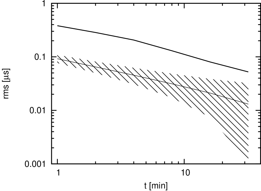
Figure 3: Comparison of achieved timing precision with the theoretically attainable precision as a function of integration time. The line in the dashed region plots the theoretical rms, equal to the mean rms obtained from $10^{5}$ different realisations of white, homoscedastic noise. This values agree with expectations based on the width of the mean pulse profile and the $S/N$. In 95% of the simulations, the rms falls within the dashed region. The confidence interval is much broader at long integration lengths because a fixed number of initial pulse profiles is used; hence, at large t, fewer independent instances remain, thus biasing the estimate.

In the above simulation, the white noise added to each simulated pulse profile is statistically independent of the noise in every other profile; in this case, as profiles of roughly equal $S/N$ are integrated together, the rms of arrival times derived from the integrated totals will be roughly proportial to $T^{-1/2}$, where T is the integration length. Consequently, the statistical independence of errors in arrival time estimates is commonly verified using a plot of residual rms as a function of integration length, as shown in Figure 3. Here, the thick line indicates the mean theoretical expectation based on $10^{5}$ simulations of $64$ ToAs derived from template with white noise added. The shaded region shows the $95\%$ confidence levels derived from the same simulations. The deviation of solid lines from $1/\sqrt{t}$ behaviour is solely due to the small number of points at longer integrations, e.g. only 2 points are available at 32 minute integration length. The fact that the observed rms follows the expected behaviour suggests that no pulse-to-pulse correlations or anti-correlations are important in our dataset. We note that the precision measured is far worse than the theoretical expectation. For example, with 32 minute integrations, we expect an rms timing residual of $\sim 13$ ns but we observe a typical value of $52$ ns. This factor of $\sim 4$ worse than the theoretical prediction implies that, if this problem was understood and fully corrected, then the same observing precision could be achieved with integrations 16 times shorter than currently required.

The above simulation does not include any self-noise or subpulse modulation; therefore, the predictions in Figure 3 are those expected from the radiometer equation (e.g. Dewey et al., 1985). However, in the real data the variance of the noise in the off-pulse region understimates the variance and completely neglects the temporal correlation of the noise in the on-pulse region; that is, the actual noise is heteroscedastic and correlated. Increasing the gain of the antenna will amplify SWIMS and while the $S/N$ calculated using only the off-pulse noise will increase the rms timing residual will not decrease. Therefore, longer integrations will be necessary to achieve a lower rms timing residual. More importantly, the SWIMS in the total intensity from subpulse modulation is spectrally correlated. Figure 4 shows a greyscale image of a single pulse from PSR J0437$-$4715 as function of pulse phase and radio frequency taken with the ATNF Parkes Swinburne Recorder (APSR; van Straten & Bailes, 2011). The emission clearly extends across the entire observed band, producing a high degree of spectral correlation of subpulse intensity fluctuations. To see if ToAs from independent bands are correlated we divided our template and each one minute observation into two independent frequency channels and determined the timing residuals for each channel separately. Figure 5 shows the timing residuals plotted against each other for one hour of data processed in this way and shows that the ToAs are highly correlated between the two channels (the average Pearson product moment correlation coefficient between the two sub-bands is $0.91$). If the subpulse modulation contribution to SWIMS had no impact on the timing residual, no such correlation would be present. In addition, the rms timing residual of each of the two sub-bands, as well as the combined rms timing residual is similar to the value obtained for the combined data. Under the assumption that the broadband subpulse properties of PSR J0437$-$4715 are responsible for the scatter in the timing residuals, increasing the observing bandwidth will not reduce the SWIMS component due to subpulse modulation.

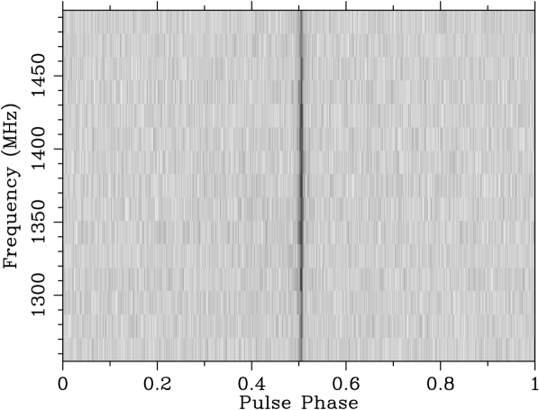
Figure 4: Greyscale image of a single pulse from PSR J0437$-$4715 as a function of pulse phase and frequency taken with the APSR instrument. We stress that (a) the subpulse persists across the whole available band, and (b) that each subpulse is very different from the average profile.

Figure 5: Timing residuals derived from two independent sub-bands every 60 seconds plotted against each other to demonstrate their remarkable degree of correlation.

The heteroscedastic and both temporally and spectrally correlated properties of SWIMS can lead to significant statistical bias in arrival time estimates derived from sources with amplified flux densities comparable to the system equivalent flux density. The following sections report on an investigation of one possible method of correcting these biases.

4 Method

As explained in the previous section, failure to account for the statistical characteristics of SWIMS leads to measurment bias and underestimation of arrival time uncertainty. In this section, we explore the use of principal component analysis (PCA) to correct the statistical bias through a series of simplified simulations. These simulations do not model the large number of impulsive intensity fluctuations; rather, the simulations demonstrate that the PCA model corrects only the arrival time bias due to profile shape variations and that no other sources of phase noise are incorrectly mitigated. An overview of PCA is given in Hyvarinen et al. (2001). We extend the analysis introduced by Demorest (2007) and then present a number of illustrative simulations that demonstrate the validity of our method and its implementation. A very similar methodology has been under development by Cordes and his collaborators since the 1990s (private communication, Cordes, 1993).

The PCA method provides a rigourous and unbiased statistical method for analysing temporally correlated variations in total intensity. For each one-minute observation of PSR J0437$-$4715  $\sim 15\times 10^{6}$ samples are integrated in each of the $N_{\rm bin}$ pulse phase bins; therefore, by the central limit theorem, the fluctuations in total intensity are well described by a multivariate normal distribution. If the distribution of these fluctuations was strongly non-normal, better performance might be achieved by a similar method using independent component analysis (Hyvarinen et al., 2001). We note that the number of pulses integrated in each minute is approximately an order of magnitude larger than the number of pulses considered in previous studies of profile stability (Helfand et al., 1975; Rathnasree & Rankin, 1995).

Assume that $N$ such observations have been made of a given pulsar. We describe the profile for the $i$’th observation as a column vector $\textbf{{p}}^{i}$. The $j$’th element, $p_{j}^{i}$, is the amplitude of the $j$’th bin in the $i$’th profile. The covariance matrix is typically computed after subtracting the mean of all observations from each observation. Here, we assume that the template, s , is a good estimate of the mean profile and, before subtraction, each observation is first adjusted to match the template using the best-fit phase shift, scale and offset as derived from the template-matching procedure used for pulsar timing (see §3). We then form the covariance matrix of the dataset by computing the outer product of template matched profiles:

$$\textbf{{C}}=\frac{\displaystyle\sum_{i=1}^{N}w_{i}\left(\textbf{{p}}^{\prime i}-\textbf{{s}}\right)\left(\textbf{{p}}^{\prime i}-\textbf{{s}}\right)^{T}}{\displaystyle\sum_{i=1}^{N}w_{i}}\;{\rm,}$$ (2)

where $w_{i}$ is the $S/N$ of the $i$’th profile, the T superscript denotes transposition and the prime superscript signifies that the profiles have been matched to the template. The resulting covariance matrix, C, is a symmetric matrix with the number of rows and columns equal to the number of bins, $N_{\rm bin}$, in each profile. We note that at least $N_{\rm bin}$ observations are necessary for C to have full rank. Furthermore, the data set should be large enough so that all potential modes of profile variation are represented.

Template matching before subtracting the standard profile removes three degrees of freedom from the shape fluctuations that are intrinsic to the pulsar signal. For example, to first order, the best-fit phase shift removes all variations that correlate with the derivative of the standard profile with respect to pulse phase. Removing variations with a certain profile shape is equivalent to projecting the $N_{\rm bin}$-dimensional vector space of the total intensity fluctuations onto the $N_{\rm bin}-$1-dimensional subspace that is orthogonal to the axis defined by that profile shape. A significant amount of the fluctuation information may be lost by this projection. However, if the best-fit phase shift were not first removed, any actual phase shifts would be misinterpreted as shape variations; therefore, this dimension must be excluded from the analysis. Similarly, the best-fit scale and offset remove variations in pulsar flux and system temperature, respectively; these fluctuations are not the focus of this work. In practice, all the data are fit for phase shift, flux scale and baseline offset and these three dimensions are always projected out of the available vector space in which the pulse profiles are described. The eigenvectors corresponding to these three dimensions all have the same eigenvalue (zero) and hence together form an eigenspace; we refer to the template matching eigenspace as the fit-space throughout the remainder of the paper.

To characterise the remaining fluctuations of the total intensity, we solve the eigenproblem of the covariance matrix. The eigenvectors $\textbf{{e}}^{j}$ define the principal axes in the $N_{\rm bin}$-dimensional vector space of profile shape variations along which the intensity fluctuations are correlated as a function of pulse phase. Sorting the eigenvectors in order of decreasing eigenvalue, $\lambda$, allows us to determine the most significant variations. The variance corresponding to each eigenvector is equal to the corresponding eigenvalue.

The eigenvectors form an orthonormal basis onto which each residual difference profile can be projected. The projection coefficient, $\alpha_{ij}$, of the $i$’th difference profile onto $j$’th eigenvector is

$$\alpha_{ij}=\left(\textbf{{p}}^{i}-\textbf{{s}}\right)^{T}\textbf{{e}}^{j}\;{\rm.}$$ (3)

These coefficients can be thought of as the residual of the $i$’th pulse profile in the basis spanned by the eigenvectors e and are often referred to as the principal components.

After the subspace projection that removes the phase shift, scale, and offset dimensions, the remaining projection coefficients for each residual profile are uncorrelated; i.e.,

$$\sum_{i=1}^{N}\alpha_{ij}\alpha_{ik}\propto\delta_{jk},$$ (4)

where $\delta_{jk}$ is the Kronecker delta. However, these coefficients may possibly be correlated with unobservable variations in the three dof that have been removed. These correlations are exploited by the technique developed in §4.1, where we introduce a new method for using these projection coefficients to correct the timing residuals for the statistical bias introduced by pulse shape variability. Simulations to confirm our algorithm are presented in §4.2.

4.1 Correcting the timing residuals: multiple regression

Demorest (2007) measured the correlation between the first projection coefficient (corresponding to the largest variance in the data) and the arrival time residuals. This was subsequently used to detect corrupted data and he has shown that it could be used to remove their deleterious effect on the timing residuals. However, his method only used the information stored in the first projection coefficient. Here we apply a multi-variate statistics method of multiple regression to simultaneously remove the effects of multiple varying components.

To predict the statistical bias in ToA estimate, $I_{i}$, caused by SWIMS we assume that there is a linear function relating this bias to the projection coefficients. We use the observed timing residuals, $R_{i}$, to determine the best-fit parameters for this function.

We wish to predict $I_{i}$ using the linear predictor

$$I_{i}=a+\textbf{{A}}^{\mn@boldsymbol{\alpha}}_{i}$$ (5)

where $a$ and A are the regression coefficients of the linear predictor. These are determined from the observed residuals by minimising the mean squared error between the predicted and observed residuals: $\sum_{i}\left(R_{i}-I_{i}\right)^{2}$. The analytic solution is given by (Johnson, 1998):

$$\textbf{{A}}=\textbf{{D}}^{-1}{\bm{\gamma}}\;{\rm,}$$ (6)

and

$$a=\nu+\textbf{{A}}^{T}{\mn@boldsymbol{\mu}}\;{\rm,}$$ (7)

where

$$\textbf{{D}}=\frac{\displaystyle\sum_{i=1}^{N}\left(\mn@boldsymbol{\alpha}_{i}-<\mn@boldsymbol{\alpha}>_{i}\right)\left(\mn@boldsymbol{\alpha}_{i}-<\mn@boldsymbol{\alpha}>_{i}\right)^{T}}{N}\;{\rm,}$$ (8)

is the covariance matrix of the projection coefficients, $\mn@boldsymbol{\gamma}$ is the vector of covariances between the residuals and the projection coefficients

$$\mn@boldsymbol{\gamma}_{j}=\left(\left(\mn@boldsymbol{\alpha}^{T}\right)_{j}-<\left(\mn@boldsymbol{\alpha}^{T}\right)_{j}>\right)\left(\textbf{{R}}-\mn@boldsymbol{\nu}\right)\;{\rm,}$$ (9)

and $\mn@boldsymbol{\nu}$ is a vector with each element equal to the mean of the observed residuals. The elements $\mu_{i}$ are the mean values of $\mn@boldsymbol{\alpha}_{i}$ and $<.>$ denotes average of vectors. The values of A and $a$ allow us to predict the bias in ToA estimation induced by pulse shape variations. This predictor has minimum mean squared error and maximum correlation with the $R_{i}$. Subtracting the predicted bias from the estimated arrival times has the potential to reduce the post-fit arrival time residual rms.

The expected improvement in timing residuals can be calculated from the projection coefficients and the observed residuals as

$$\frac{\sigma^{\prime}}{\sigma}=\sqrt{1-\rho^{2}}\;{\rm,}$$ (10)

where

$$\rho=\sqrt{\frac{{\mn@boldsymbol{\gamma}}^{T}\textbf{{D}}^{-1}{\mn@boldsymbol{\gamma}}}{\sigma^{2}}}.$$ (11)

Here $\sigma^{\prime}$ is the rms timing residual for ToAs with the bias removed and $\rho$ is called the population multiple correlation coefficient.

It is necessary to restrict the number of eigenvectors to model only pulse variability. Many approaches have been put forward in the literature for determining the number of significant principal axes (Johnson, 1998). We introduce a new parameter, $\xi_{j}$, which is the Pearson’s product moment correlation coefficient between the the timing residuals, R, and the projection coefficients onto the $j$’th eigenvector, that is the $j$’th row of $\mn@boldsymbol{\alpha}$. The standard deviation of non-significant $\xi$ values is determined. Significant values are identified using a Tukey’s bi-weighting scheme starting with an initial guess of the standard deviation obtained from the median absolute deviation. The resulting standard deviation of the $\xi$ values is a robust and resistant estimator. For more details see Andrews (1972) and Hoaglin et al. (1983). Starting from the last correlation coefficient we search for three consecutive $\xi$ values that are more than three times this measured standard deviation. The number of the eigenvectors used in all subsequent processing is equal to the index of last of these three values, when counting from one. For cases in which fewer than three $\xi$ values are significant, we compare the results of using only one eigenvector with those of using the first five.

An implementation of this method is publicly available as a part of the PSRCHIVE suite. The relevant application is called “psrpca” and it requires the GNU Scientific Library to work.

4.2 Simulations

To confirm that our method correctly detects pulse shape variations that can be used to correct statistical bias in ToA estimation, we carry out three simulations of data with noise in the third regime (i.e., SWIMS). In every simulation, each observed profile is replaced by a copy of the template profile plus white noise and additional varying components. The amount of white noise is set such that in many random realisations of the simulated observation the mean $S/N$ of the simulated profile would match that of the given observation. Although there can be several subpulses per pulse period, we illustrate the technique using a simple model in which only a single subpulse is added per minute of observation. Note that this procedure does not affect the observing parameters (such as frequency, observation time etc.) which are held fixed at the values in the actual observations. The resulting simulated observations are cross-correlated with the template to form ToAs (and hence residuals) in exactly the same manner as the actual observations.

We initially tested the trivial cases of simulated data with white radiometer noise only with or without arbitrary phase shifts applied to the data. As expected, no significant eigenvectors were detected in either case. Attempting to correct the residuals regardless of that yields no significant improvement in the rms timing residual. These two cases demonstrate that our method will not artificially decrease the arrival time residual arising from white noise or arbitrary phase shifts. The latter could arise from any phase shift such as that due to a gravitational wave and it is important that such signal is not removed by the PCA.

4.2.1 Simulation 1: Single, fixed component

Figure 6: First eigenvector for simulation with white noise, arbitrary shifts and a von Misses component on top of the template profile. Notice that this eigenvector does not look purely like von Mises distribution as it has to be orthogonal to the fit-space.

Pulsar emission is often modelled as consisting of multiple Gaussian components (e.g. Kramer et al., 1999). Many pulsars show mode changing where one or more components are active for only a finite amount of time (Wang et al., 2007). To verify that the bias introduced by a single “mode changing” component can be detected and corrected, we now include an extra component in the profile that varies in amplitude. This component is created from a von Mises function (which is a periodic analog to a Gaussian distribution) with a normally distributed amplitude that has a mean value of zero and an rms of 3% of the peak template flux. This component is centred at pulse phase $0.504$ and has a concentration parameter equal $0.113{\rm bins}^{-2}$. The resulting weighted rms timing residual was $255$ ns and $\chi^{2}/dof=14.4$, while without the additional component the same realisation of white noise leads to an rms of $59$ ns and a $\chi^{2}/dof$ of $1.0$. We emphasise that this increased rms residual and high $\chi^{2}/dof$ is due solely to the pulse shape variations and therefore should be detected and corrected using our method.

We obtain a significant first eigenvalue. The automatic determination of useful eigenvectors fails, as there is only one significant eigenvector, associated with the introduced profile variation. Figure 6 shows the first eigenvector, which is different from the introduced component as it is projected onto the $N_{\rm bin}-3$ dimensional space, in which the three dimensions corresponding to the fit-space are removed. Although these degrees of freedom have been removed, the residual shape variation is still highly correlated with the ToA residual, as discussed above. Correcting the residuals using the one significant eigenvector reduces the rms residual to $67$ ns and the $\chi^{2}/dof$ to $1.0$. We note that this improvement agrees very well with prediction from equation 10. We calculate reference residuals by simulating and timing data without any additional components but with the same realisation of white noise as in the simulation with the varying component. As expected the corrected residuals are highly correlated with the reference residuals (correlation coefficient of $0.93$). This indicates that we have recovered most of the signal in the original residuals and have removed the effect of the pulse variability.

We note that after removing the bias in ToA residuals the weighted rms timing residual is almost the same as in the case of reference residuals; however, the $\chi^{2}/dof$ can be smaller than that of the reference residuals because the ToA uncertainties have increased. The total intensity fluctuations decrease the cross-correlation between the observation and the template, thereby increasing the estimated uncertainty (see equation A10 from Taylor, 1992).

In order to check the effect of using a different number of eigenvectors to correct the timing residuals, we re-analysed the data using five eigenvectors. In this case the rms residual and $\chi^{2}/dof$ were $64$ ns and $0.92$ respectively. The corrected residuals are still pleasingly highly correlated with the reference residuals. We therefore conclude that our result is not highly sensitive to the number of eigenvectors used, but care needs to be taken when choosing that number.

In addition, we also tested an extended version of this simulation, where arbitrary phase shifts were included to simulate, e.g., the effect of gravitational waves. As expected, only the bias in the timing residuals due to the introduced profile variation is removed and the arbitrary phase shifts remain unaffected. Again, the residuals are highly correlated with reference residuals where the same realisations of white noise and arbitrary shifts were introduced.

4.2.2 Simulation 2: Multiple, fixed components

Table 1: Parameters of the multi-component simulation.

	1	2	3	4	5	6
centre	$0.504$	$0.496$	$0.512$	$0.524$	$0.509$	$0.520$
amplitude	$0.74\%$	$0.36\%$	$0.86\%$	$1.4\%$	$0.7\%$	$0.4\%$
$\kappa$	$0.452$	$0.164$	$0.098$	$0.050$	$0.577$	$0.104$

The previous simulation dealt with only a single varying component while many pulsars can emit radiation simultaneously from several components. Even if only one of the multiple components was present in each rotation of the pulsar, several components would be present after integration over multiple pulse periods. To demonstrate again that PCA and multiple regression do not remove phase shifts that are not caused by pulse shape variations, we now introduce six von Mises functions whose amplitudes are allowed to vary independently. The parameters of these components are presented in Table 1, where centre is the central phase of a von Mises component in pulsar turns; amplitude is the rms of the amplitude distribution of given component, in units of the template’s peak flux; and $\kappa$ is the concentration parameter of the von Mises distribution in units of ${\rm bin}^{-2}$. We also apply arbitrary phase shifts after adding the varying components. This leads to a weighted rms residual of $372$ ns and $\chi^{2}/dof$ of $32.1$. Note that the reference residuals obtained from a simulation with the same realisation of white noise and arbitrary phase shifts, but no additional components, have an rms of $206$ ns and $\chi^{2}/dof$ of $12.2$ due to the arbitrary phase shifts; i.e., we do not expect the rms to be of the same order as the ToA measurement error after bias removal.

Our method gives corrected residuals with weighted rms residual of $216$ ns ($\chi^{2}/dof=10.8$) and they are highly correlated with the reference residuals. With multiple components the bias is not completely removed because more than one projection coefficient correlates with the arrival time residual and these projection coefficients may not be statistically independent of each other. Nevertheless, significant improvement in the rms residual and in the $\chi^{2}/dof$ is apparent and much of bias is removed. The additional shifts, corresponding to unmodelled timing noise processes are still unaffected; i.e., the post-correction residuals are highly correlated (correlation coefficient of $0.87$) with the reference residuals.

4.2.3 Simulation 3: Single, random component

We now consider a possibly more realistic case of the pulsar emission being erratic and distributed in phase over the whole region in which the average profile is visible; this case corresponds to the stochastic nature (Cordes & Downs, 1985; Cordes, 1993) of modulated pulses. In this simulation we allow a single von Mises component per simulated profile to be centred anywhere in within the central peak (central phase uniformly distributed between $0.479$ and $0.518$). The concentration parameter of the component is uniformly distributed between $0.055$ and $1.386$ ${\rm bin}^{-2}$. The amplitude of this component is normally distributed with an rms equal to $2.3\%$ of the intensity of the template at the centre phase of the component. This value is chosen in order that the resulting rms timing residual is $380$ ns and $\chi^{2}/dof$ value of $35.1$, both very close to the observed values for PSR J0437$-$4715.

Multiple significant eigenvectors are detected, with the number varying between different realisations from 10 to 50. Correcting the residuals reduces the rms to $266$ ns and $\chi^{2}/dof$ to $17.2$. We note that in this simulation no arbitrary shifts were included and therefore we conclude that the PCA method has failed to completely remove the bias in ToAs (and hence in residuals) induced by this kind of erratic shape variation. As explained in §4 some fraction of the fluctuation power is lost during the vector subspace projection effected by removing the best-fit shift, scale, and offset. As before, for data integrated over multiple pulse periods, more than one varying component per pulse profile would be present and this could make it even more difficult to remove the bias in ToAs.

5 Results

Figure 7: Distribution of correlation coefficients between the residuals and projection onto eigenvectors for the actual observations, shown by open circles. Several correlation coefficients are more than 3 standard deviations (denoted by the dashed lines) above the background noise level. Only the first 150 correlation coefficients are shown, the rest of the correlation coefficients looking very similar as the last shown. The crosses are showing the corresponding eingenvalues normalised by their sum, multiplied by a factor of 10 and offset by $-0.45$ for clarity of the figure.

Applying our method to the observed dataset of 1145 profiles leads to:

• the detection of significant pulse shape variations with at least ten significant eigenvectors,

• a reduction in rms timing residual from $372$ ns to $294$ ns and a reduction in $\chi^{2}/dof$ from 33.8 to 21.1.

Figure 8: First three eigenvectors for the observed data. We show only the central part of the profile for clarity. The vertical thick lines separate the eigenvectors. The dashed line represents the scaled template added for reference.

The first 150 values of $\xi$ are plotted in Figure 7 which indicates that around 10 eigenvectors significantly correlate with the observed residuals while the rest are consistent with being white noise. The choice of exact number of eigenvectors would be difficult to make without the rigourous criteria described before. In Figure 8, we present the three most significant eigenvectors overlaid on the pulsar template profile. The detection of significant eigenvalue-eigenvector pairs is a direct consequence of temporally correlated fluctuations in total intensity; i.e., significant shape variations are detected. As discussed in §1, §2, and §3, it is likely that such variations originate from the pulse-to-pulse variations of the pulsar emission. The most significant variation occurs at phase $0.497$, in the main peak of the pulse profile. The majority of other significant eigenvectors peak around the main and second highest peak in the mean profile. One exception is the 10th eigenvector that peaks at phase $0.385$, that is in the local peak on the left hand side of the main peak.

Using the 10 most significant eigenvectors to correct the bias in arrival time estimates, the rms timing residual was reduced by $20\%$ and $\chi^{2}/dof$ was reduced by $36\%$. Only $3\%$ of the variance in the timing residuals can be attributed to the most significant eigenvector; therefore, multiple regression is required to provide the best estimate of statistical bias. The third simulation has demonstrated that pulse profile variability can introduce bias in ToAs that cannot be removed completely using our method and the timing residuals after bias correction are still biased. Therefore, even though only $20\%$ of the rms timing residual is corrected, there need not be another explanation for the remaining timing noise. For completeness, other effects that might contribute to the rms of timing residuals are discussed in the next section.

To investigate if the intensity fluctuations arise from a stationary stochastic process, at least in the wide sense, we used five hours of observations of PSR J0437$-$4715 during July 2009 obtained using the same observing system as described in §3. These additional data were processed to form pulse profiles, arrival times and timing residuals in exactly the same way as our main data set. We used the eigenvectors and regression coefficients obtained above to correct these July 2009 timing residuals. We again achieved a 22% decrease in the rms timing residual from $380$ ns to $296$ ns and the $\chi^{2}/dof$ was reduced by $36$% from $39.1$ to $24.9$. The fractional improvement is similar to before, implying that the covariance matrix and hence profile variability is stationary in time and that after the regression coefficients and eigenvectors have been determined for one dataset they can subsequently be applied to other observations of the same pulsar obtained with the same instrumentation and observing parameters.

6 Discussion

We first discuss the method that we have introduced to search for and correct pulse shape variability. Second, we discuss the astrophysical implications of broad-band profile shape variations intrinsic to the pulsar.

6.1 Discussion of the method

It is clear from the simulations that our method successfully detects significant pulse shape variations and partially corrects the bias induced in timing residuals due to such variations in many cases. The method has certain limitations. First, in order for the covariance matrix, C, to have full rank, the method requires at least $N_{\rm bin}$ observations. With fewer observations than phase bins, it may be necessary to average adjacent phase bins, or, if prior knowledge suggests that the pulse variability occurs in only a restricted region then only these bins could be included in the analysis. If full phase resolution is required then the covariance matrix can be determined, but not all of the eigenvectors can be calculated. Alternatively, following Demorest (2007), the PCA method can be developed in the frequency domain using only the significant harmonics thus reducing the number of required observations.

A large number of observations is desirable for two reasons. Firstly, dividing a fixed observing time into smaller intervals provides a greater number of estimates of the pulse profile, thereby increasing the $S/N$ of the covariance matrix estimate. Secondly, even for $N>N_{\rm bin}$ our method is limited by the SEFD present in all observations. Such noise will reduce the precision with which the eigenvectors may be determined, reducing their ability to fully describe the shape variations. For instance, in the timing residuals of simulations with only white radiometer noise added, even though no significant eigenvalues were measured, the rms timing residual is reduced by a negligible amount when using just a few eigenvectors. When all of the eigenvectors are included in the bias removal, the effects of white noise are artificially reduced. This occurs because the white radiometer noise affects the regression coefficients $a$ and A in equation 5. Since the eigenvectors are measured using the data that are being “corrected’, the noise in the eigenvectors correlates with the noise in the data. This is similar to the “self-standarding” effect that arises when the mean of a set of observed profiles is used as the template to derive arrival times from the same data, as described in Appendix A of Hotan et al. (2005). Applying the eigenvectors to a completely independent data set leads to no significant change to the timing residuals as the noise in the data no longer correlates with noise in the eigenvectors. The degree of correlation between individual residual profiles and the white-noise eigenvectors may also be reduced by increasing the number of observations from which the covariance matrix C is estimated. If the eigenvectors are obtained from the data to be corrected, then it is essential to apply the rigourous criteria described in §4.1 to choose only the significant eigenvectors.

Many pulsar observations are affected by radio frequency interference (RFI) and the measured eigenvectors are extremely sensitive to the presence of RFI in the data. As pointed out by Demorest (2007), PCA is also a sensitive and robust method for detecting RFI and other types of data corruption and distortions. It is therefore essential that the data used in forming the eigenvectors are unaffected by RFI. In our case nearly $32\%$ of the pulse profiles had to be rejected. RFI might also be mitigated through the use of a robust estimator of the covariance matrix, such as the minimum covariance determinant estimator (Hubert & Debruyne, 2010).

In contrast to more traditional applications of the PCA method, our method relies on first aligning each pulse profile to the template using the best-fit phase shift, scale, and baseline offset. As a result of this fit, the last three eigenvalues are several orders of magnitude smaller (i.e., close to zero) and the corresponding eigenvectors spanning the fit-space are highly correlated with the template profile, its phase derivative, and the baseline offset or their linear combinations. In other words, the profiles are originally described in an $N_{\rm bin}$ dimensional vector space and the fit projects the data onto $N_{\rm bin}-3$ dimensional vector space in which the fit-space has been removed. This removes three degrees of freedom from the remaining eigenvectors and limits the efficacy of the correction scheme presented in this paper because the fit-space component of the intrinsic shape fluctuations has been removed. Consequently, the bias due to any intrinsic shape fluctuations that correlate with these eigenvectors cannot be fully corrected. This is especially important in the case of profile variations correlated with the template derivative as such variations will introduce most bias in the ToAs. Only the total intensity fluctuations that are orthogonal to the fit-space contribute to the predictor computed in equation 5. The degree to which such fluctuations are correctable depends on how strongly they correlate with these three eigenvectors and the degree of correlation between the remaining projection coefficients and the arrival time residual.

We note that our work has implications for any relevant template matching algorithms. Such algorithms normally assume that the errors in the measurements of intensity are homoscedastic and uncorrelated. Our detection of profile variations implies that the errors are, in fact, heteroscedastic and correlated. We note that including the covariance matrix, which carries the information about the correlation and heteroscedasticity of the noise, into the template matching algorithms will yield better estimates of ToA uncertainty. It may also remove the necessity of correcting the residuals by the means described in this paper because any statistical biases caused by the intensity fluctuations might be removed at the time of ToA determination. This is similar to the Cholesky decomposition which can remove bias in estimation of various parameters, such as parallax, when estimating from residuals with red noise present (Coles et al., 2011). Examples of template matching algorithms are the standard ToA derivation algorithm presented by Taylor (1992) and the matrix template matching algorithm that allows all Stokes parameters to be used in the ToA estimation (van Straten, 2006). An unbiased generalisation of template matching would be a logical extension of this work.

6.2 Application to PSR J0437$-$4715

Using one-minute integrations of PSR J0437$-$4715, we have detected shape fluctuations that we attribute to the stochastic subpulse structure of the pulsar emission. However, for many timing applications, the exact cause of the pulse shape variations is irrelevant. This technique can be used to correct bias and improve sensitivity to any phenomena that do not induce shape variations. For instance, in order to place a limit on the existence of a gravitational wave background (e.g. Jenet et al., 2006) some methods compare the amount of power in the timing residuals with the power predicted to be induced by gravitational waves. Such waves will not affect the pulse profile shape. Therefore, reducing the rms timing residuals by accounting for pulse shape variations allows an improved limit on the existence of a gravitational wave signature to be obtained. We note that our correction method does not remove any of the signal induced by gravitational waves or any other phase shift of the pulsar profile, as verified by the simulations.

The long term timing of PSR J0437$-$4715 shows significant low frequency structure present in the residuals (e.g. Verbiest et al., 2008). Such red timing noise is a common type of non-Gaussianity (in general any asymmetric distribution will have a similar effect) in the timing residuals. It is important to determine the best predictor for correcting the residuals based on a short data span, as it will be less affected by any non-Gaussian noise. In the presence of non-Gaussian components, the best predictor will be affected as the correlation coefficients $\xi$ between the residuals and projection coefficients will be biased toward zero. Presence of Gaussian noise (or any other symmetrically distributed noise) will increase the uncertainty in the estimate of $\xi$ values but will not bias them.

The timing residuals for our Parkes observations are only partially corrected by our new method. We have demonstrated that partial correction does not necessarily imply the existence of other sources of scatter in ToA residuals that do not affect the pulse shape. At the same time it is not possible to completely exclude the existence of other effects such as hardware or software errors that are affecting the timing residuals at a lower level. Other possible effects that can increase the rms timing residual are described in detail by Cordes & Shannon (2010); Liu et al. (2011). Such issues are beyond the scope of this paper, which concentrates solely on the pulse shape variability. We note that if any other non-white process affecting the residuals could be corrected, the residuals induced by profile shape variations could be removed more completely as the estimates of $\xi$ are affected by the presence of phase noise.

We stress that the intrinsic shape variations lead to the heteroscedastic and correlated component of the SWIMS. The uncorrelated component, originating from the standard radiometer noise in the weak source limit and the self-noise, is described by the diagonal of the covariance matrix C while the temporally correlated part is described by the off diagonal elements. However, whatever phenomena contribute to the correlated component will naturally also contribute to the diagonal of the covariance matrix. As the self-noise and subpulse modulation are all measured and described simultaneously by the covariance matrix, it is natural to consider them all as one phenomenon, which we called SWIMS throughout this paper. Two details of covariance matrix we would like to stress are that: a) it does not contain any information about the spectral correlation of the noise and b) the measured covariance matrix also contains a contribution from the SEFD which can be subtracted if necessary. Extrinsic sources can also introduce a heteroscedastic and correlated component of noise, such as lightning strikes, other types of RFI or some instrumental effects, such as non-linearity of the backends. The effects of impulsive interference should be present across the whole pulse profile as they occur randomly in pulse phase. After careful removal of RFI, the measured eigenvectors are consistent with white noise outside the mean profile (see §5).

As shown in Figure 6, interpretation of the eigen-vectors derived from the covariance matrix is complicated by the fact that the fit-space has been projected out of the $N_{\rm bin}$-dimensional space of the shape variations. To investigate the structure of the shape variations prior to this projection, one can make the assumption that the pulsar timing model accurately predicts pulse phase (at least over the time-scale of the observations) and compute the covariance matrix of observed profile residuals after template matching by varying only the scale and offset (i.e. no phase shift). In this case, the covariance matrix contains the cyclic, phase-resolved autocorrelation [autocorrelation function (ACF)] of the intensity fluctuations. The mean ACF computed by summing elements along the diagonals of this matrix is plotted in Figure 9. The characteristic width of ACF, as determined by fitting a Laplace function, is equal to 67 $\mu$s, which is consistent with the average width of microstructure events reported by Jenet et al. (1998). For comparison, the mean ACF formed from the covariance matrix used for bias removal (i.e. best-fit phase shift removed) is also plotted with a dashed line. A large fraction of the fluctuation power is removed by fitting for the phase shift during template matching. The phase shift fit removes variations that correlate with the template derivative, and the autocorrelation of the template derivative reaches its first minimum (below zero) at roughly the width of the pulse profile (around 140 $\mu\rm{s}$). This corresponds with the first dip seen in the ACF formed from data in which no phase shift has been removed; no dip is present in the ACF formed after fitting for phase shift. The measured ACF may be affected by other non-intrinsic effects, especially those related to propagation through interstellar medium (ISM; Smits et al., 2003). We argue below that the ISM is not an important factor in considerations of PSR J0437$-$4715. The ACF shows a periodic ripple (most apparent at large phase lags), which is believed to be an instrumental artefact; it has a period of roughly $100\;\mu\rm{s}$. Its origin is currently unknown. Preliminary analysis of data from another instrument (Caltech Parkes Swinburne Recorder 2, CPSR2; Bailes, 2003; Hotan, 2006) confirms that this effect is intrinsic to PDFB3 as the ACF calculated from CPSR2 has no periodic ripple present. The pulse profile variations are still detected thus confirming their origin as intrinsic to the pulsar.

Figure 9: The ACF calculated with the assumption of the timing model accurately predicting the pulse phase over the course of observations (solid line) and without this assumption, i.e., when performing a full template matching (dashed line). The width of the ACF is determined by the characteristic width of single pulses (Rickett, 1975). The SEFD contributes an unresolved spike at zero lag, which is scaled to unit height for the solid line and the dashed line uses the same scaling factor.

The interstellar medium can also introduce shape variations, such as broadening of the pulse profile, which increases quadratically with DM and decreases quartically with frequency. Given the very low ${\rm DM}=2.64$ cm^-3pc and the observing wavelength $\sim 20$ cm used in this work, the expected variations in the pulse width for PSR J0437$-$4715 due to broadening are of the order of $1$ ns (Bhat et al., 2004; Gwinn et al., 2006). Interstellar scintillation combined with frequency dependence of the pulse profile can also lead to fluctuations of ToAs. As shown in Figure 5 the residuals are highly correlated when estimating the ToAs from two separate frequency channels. This high correlation implies that diffractive narrow-band interstellar scintillation is not responsible for the additional scatter. As we observe variations on a time-scale of minutes it is unlikely that broadband refractive scintillation is a contributing factor to the observed pulse shape changes as the time-scale for such variations is of the order of $1000$ s (Gwinn et al., 2006). Based on the high degree of correlation between arrival times measured in separate bands (Figure 5) and the observed broadband nature of single pulses (Figure 4), we conclude that the intensity fluctuations are correlated over wide bandwidths. Consequently, increasing the bandwidth does not increase the timing precision. Only active mitigation or longer integrations can reduce the timing rms if the fluctuations of total intensity are indeed the main cause of the arrival time variations that greatly exceed the predicted uncertainty. Simultaneous multifrequency observations of PSR J0437$-$4715 would help to determine if the shape variations are persistent over very wide bands. Some observations to date have shown that the giant pulses from Crab extend over GHz bandwidths (Sallmen et al., 1999; Hankins et al., 2003; Hankins & Eilek, 2007). Another group has shown that the single pulses in PSR B0329$+$54 persist across $1.3$ GHz (Karastergiou et al., 2001) but this may not be true for all subpulse structure in the general population of pulsars.

It is also worth considering the impact of polarization variations on arrival time estimates. Emission from PSR J0437$-$4715 is highly polarised and a sudden change in the position angle of the linear polarisation occurs near the peak in the total intensity profile (as noted by Navarro et al., 1997). This implies that poor polarisation calibration will lead to significant profile changes, as quantified by van Straten (2006). For a single dish that is not equatorially mounted, these variations occur on time-scale of hours. Pulse profile shape changes detected by Vivekanand et al. (1998) were argued to be caused by calibration errors (Sandhu et al., 1997). Even though we detect fluctuations of the total intensity pulse profile on much shorter time-scales, we investigated if this was the case in our data as well. We studied the bias in timing residuals induced by the measured pulse shape variation as a function of parallactic angle. We found that there was no dependence between these two quantities. We also applied the PCA to uncalibrated data and a correlation between the induced bias $I$ and the parallactic angle was readily apparent.

We conclude that the shape variations are more likely to originate at the pulsar rather than in the observing hardware or from interference. The polarisation calibration has been performed sufficiently to alleviate at least minute-time-scale fluctuations and does not introduce detectable pulse shape variations. The interstellar medium is also unlikely to cause such variations. Even if the detected variability is not intrinsic, the presented methodology remains valid. The intrinsic variation is expected from the stochastic subpulse structure and will be detectable if the pulsar is bright enough.

Since the detected variations are likely to be intrinsic to the pulsar, a question arises whether the profile variations in PSR J0437$-$4715 are related only to SWIMS or if they are due to mode changing. We searched for clustering in the space spanned by the projection coefficients onto the ten significant eigenvectors by applying a friends-of-friends algorithm known from n-body simulations to identify dark matter haloes (Davis et al., 1985). We did not find any evidence of clustering in this space and hence conclude that the pulse profile variations are not due to mode changing.

We would like to stress the importance of our work for the next generation telescopes, which are likely to provide more sensitivity than currently available. With its huge collecting area of 1 ${\rm km}^{2}$, the Square Kilometre Array (SKA) is expected to revolutionise pulsar astronomy. One of the Key Science Projects of the SKA requires pulsar observations with the highest possible timing precision (Kramer et al., 2004). It is assumed that the SKA will observe of the order of $100$ millisecond pulsars with an rms timing precision better than $100$ ns. With the SKA’s phenomenal sensitivity, the $S/N$ of a pulse profile should be $>$1000 on a time-scale of only minutes for many pulsars (compared with many hours with the Parkes telescope). The short observing times required to achieve such high $S/N$ ratios would allow the SKA to observe multiple pulsars in a short time. However, the increased sensitivity of next-generation telescopes will also increase the relative importance of SWIMS as the radiometer noise is decreased. If the intrinsic pulse shape variations that we have detected for PSR J0437$-$4715 are typical of many MSPs at the observing frequency being used, they will induce a floor on timing precision that can be ameliorated only with longer integration times and active mitigation using methods such as the one presented in this work. Cordes & Downs (1985) demonstrated that, for the majority of their sample of 24 pulsars, timing precision is likely to be limited by phase jitter. No millisecond pulsars were included in this sample. Shannon & Cordes (2010) later argue that the timing noise of millisecond pulsars is similar to that of classical pulsars, only much smaller. Although SWIMS has not yet been detected in most pulsars, it is likely to be revealed with better instrumentation, more sensitive telescopes or longer data spans. Since the detected pulse shape variations are likely to be very broadband, increasing bandwidth will not reduce the bias introduced by SWIMS. This must be considered when predicting the potential science of current and future pulsar timing array projects and the observing time and strategy necessary to achieve the stated goals. For example, with an SKA-like telescope, if many pulsars in a timing campaign are limited by SWIMS, then it is better to observe multiple pulsars simultaneously with fraction of the array for longer time rather than using full sensitivity to observe pulsars one by one for a short time. Some proposed astrophysical experiments demand extremely accurate ToAs over short intervals of the order of minutes, such as when a pulsar passes behind black hole in a close binary. SWIMS will make such experiments difficult or impossible.

The relative importance of the correlated component of SWIMS is also expected to vary between pulsars as it depends on intrinsic subpulse emission properties and the shape of the average pulse profile. The fractional improvement in rms timing residual is expected to vary from case to case and it can be hoped that for pulsars with simpler and/or narrower profiles, variability in the subpulse structure will be less severe. As demonstrated by our first simulation, in simple cases our method works very well and can completely remove the statistical bias in ToAs for some pulsars. Our method can be used to identify pulse profile modes which can lead to improved timing.

We note that, for current telescopes, equation 1 is a good approximation for the vast majority of MSPs, which have time averaged mean flux densities an order of magnitude smaller than PSR J0437$-$4715. For example, in the Parkes Pulsar Timing Array sample, fluxes vary between $1.3$ and $13.8$ mJy (see Table 2 of Yan et al., 2011) with a median value of $2.4$ mJy, compared to the mean value of $150$ mJy for PSR J0437$-$4715. Consequently, the profile variability arising from SWIMS has been neglected to date. We note that future telescopes like the SKA are likely to perform timing array experiments at higher frequencies to avoid some of the problems caused by the interstellar medium. Whether SWIMS will be a crucial limitation to precision timing for the majority of pulsars at all observing frequencies remains to be seen.

7 Conclusion

We have developed an extended principal component analysis method that is applicable to searching for pulse shape variations in pulse profiles. Applying this method to PSR J0437$-$4715 shows the presence of pulse profile variability that is likely to be intrinsic to the pulsar. The statistics of this variability are consistent over many months. The detection of significant intensity fluctuations implies that self-noise may be a limiting factor for timing precision of PSR J0437$-$4715 for current generation of telescopes. Future technological developments including construction of larger antenna and increased instrumental bandwidth will not improve timing precision as the subpulse structure is a source-intrinsic broadband phenomenon. However, the effects of SWIMS can be partially corrected by the method presented in this work and the proposed generalised template matching.

References

- Andrews (1972) Andrews D., 1972, Robust Estimates of Location: Survey and Advances. Princeton University Press, Princeton
- Arzoumanian (1995) Arzoumanian Z., 1995, PhD thesis, Princeton University
- Backer (1970) Backer D. C., 1970, Nature, 228, 1297
- Backer & Sallmen (1997) Backer D. C., Sallmen S. T., 1997, AJ, 114, 1539
- Bailes (2003) Bailes M., 2003, in Astronomical Society of the Pacific Conference Series, Vol. 302, Radio Pulsars, M. Bailes, D. J. Nice, & S. E. Thorsett, ed., p. 57
- Bailes (2010) —, 2010, in IAU Symposium, Vol. 261, IAU Symposium, S. A. Klioner, P. K. Seidelmann, & M. H. Soffel, ed., Cambridge Univ. Press, Cambridge, UK, pp. 212–217
- Bartel et al. (1982) Bartel N., Morris D., Sieber W., Hankins T. H., 1982, ApJ, 258, 776
- Bhat et al. (2004) Bhat N. D. R., Cordes J. M., Camilo F., Nice D. J., Lorimer D. R., 2004, ApJ, 605, 759
- Boynton et al. (1972) Boynton P. E., Groth E. J., Hutchinson D. P., Nanos Jr. G. P., Partridge R. B., Wilkinson D. T., 1972, ApJ, 175, 217
- Britton (2000) Britton M. C., 2000, ApJ, 532, 1240
- Cairns (2004) Cairns I. H., 2004, ApJ, 610, 948
- Cognard et al. (1996) Cognard I., Shrauner J. A., Taylor J. H., Thorsett S. E., 1996, ApJ Lett, 457, L81
- Coles et al. (2011) Coles W., Hobbs G., Champion D. J., Manchester R. N., Verbiest J. P. W., 2011, MNRAS, in press
- Cordes (1980) Cordes J. M., 1980, ApJ, 237, 216
- Cordes (1993) —, 1993, in Astronomical Society of the Pacific Conference Series, Vol. 36, Planets Around Pulsars, J. A. Phillips, S. E. Thorsett, & S. R. Kulkarni, ed., pp. 43–60
- Cordes & Downs (1985) Cordes J. M., Downs G. S., 1985, ApJS, 59, 343
- Cordes & Helfand (1980) Cordes J. M., Helfand D. J., 1980, ApJ, 239, 640
- Cordes & Shannon (2010) Cordes J. M., Shannon R. M., 2010, ArXiv e-prints
- Davis et al. (1985) Davis M., Efstathiou G., Frenk C. S., White S. D. M., 1985, ApJ, 292, 371
- Demorest (2007) Demorest P. B., 2007, PhD thesis, University of California, Berkeley
- Dewey et al. (1985) Dewey R. J., Taylor J. H., Weisberg J. M., Stokes G. H., 1985, ApJ Lett, 294, L25
- Drake & Craft (1968) Drake F. D., Craft Jr. H. D., 1968, Science, 160, 758
- Durdin et al. (1979) Durdin J. M., Large M. I., Little A. G., Manchester R. N., Lyne A. G., Taylor J. H., 1979, MNRAS, 186, 39P
- Foster & Backer (1990) Foster R. S., Backer D. C., 1990, ApJ, 361, 300
- Groth (1975a) Groth E. J., 1975a, ApJS, 29, 443
- Groth (1975b) —, 1975b, ApJS, 29, 453
- Groth (1975c) —, 1975c, ApJS, 29, 431
- Gwinn (2004) Gwinn C., 2004, PASP, 116, 84
- Gwinn (2001) Gwinn C. R., 2001, ApJ, 554, 1197
- Gwinn (2006) —, 2006, PASP, 118, 461
- Gwinn et al. (2006) Gwinn C. R., Hirano C., Boldyrev S., 2006, A&A, 453, 595
- Gwinn & Johnson (2011) Gwinn C. R., Johnson M. D., 2011, ApJ, 733, 51
- Gwinn et al. (2011) Gwinn C. R., Johnson M. D., Smirnova T. V., Stinebring D. R., 2011, ApJ, 733, 52
- Hankins & Eilek (2007) Hankins T. H., Eilek J. A., 2007, ApJ, 670, 693
- Hankins et al. (2003) Hankins T. H., Kern J. S., Weatherall J. C., Eilek J. A., 2003, Nature, 422, 141
- Hankins et al. (1993) Hankins T. H., Moffett D. A., Novikov A., Popov M., 1993, ApJ, 417, 735
- Helfand et al. (1975) Helfand D. J., Manchester R. N., Taylor J. H., 1975, ApJ, 198, 661
- Helfand et al. (1980) Helfand D. J., Taylor J. H., Backus P. R., Cordes J. M., 1980, ApJ, 237, 206
- Hellings & Downs (1983) Hellings R. W., Downs G. S., 1983, ApJ Lett, 265, L39
- Hoaglin et al. (1983) Hoaglin D. C., Mosteller F., Tukey J. W., eds., 1983, Understanding robust and exploratory data analysis, Wiley series in probability and mathematical statistics. Wiley-Interscience
- Hobbs et al. (2010) Hobbs G., Coles W., Manchester R., Chen D., 2010, ArXiv e-prints
- Hobbs et al. (2011) Hobbs G., Miller D., Manchester R. N., Dempsey J., Chapman J. M., Khoo J., Applegate J., Bailes M., Bhat N. D. R., Bridle R., Borg A., Brown A., Burnett C., Camilo F., Cattalini C., Chaudhary A., Chen R., D’Amico N., Kedziora-Chudczer L., Cornwell T., George R., Hampson G., Hepburn M., Jameson A., Keith M., Kelly T., Kosmynin A., Lenc E., Lorimer D., Love C., Lyne A., McIntyre V., Morrissey J., Pienaar M., Reynolds J., Ryder G., Sarkissian J., Stevenson A., Treloar A., van Straten W., Whiting M., Wilson G., 2011, PASA, in press
- Hobbs et al. (2006) Hobbs G. B., Edwards R. T., Manchester R. N., 2006, MNRAS, 369, 655
- Hotan (2006) Hotan A. W., 2006, PhD thesis, Centre for Astrophysics and Supercomputation, Swinburne University of Technology
- Hotan et al. (2004a) Hotan A. W., Bailes M., Ord S. M., 2004a, MNRAS, 355, 941
- Hotan et al. (2005) —, 2005, MNRAS, 362, 1267
- Hotan et al. (2004b) Hotan A. W., van Straten W., Manchester R. N., 2004b, Publ. Astron. Soc. Aust., 21, 302
- Hubert & Debruyne (2010) Hubert M., Debruyne M., 2010, Wiley Interdisciplinary Reviews: Computational Statistics, 2, 36
- Hyvarinen et al. (2001) Hyvarinen A., Karhunen J., Oja E., 2001, Independent Component Analysis. John Wiley and Sons, New York
- Jenet et al. (1998) Jenet F. A., Anderson S. B., Kaspi V. M., Prince T. A., Unwin S. C., 1998, ApJ, 498, 365
- Jenet et al. (2001) Jenet F. A., Anderson S. B., Prince T. A., 2001, ApJ, 546, 394
- Jenet et al. (2006) Jenet F. A., Hobbs G. B., van Straten W., Manchester R. N., Bailes M., Verbiest J. P. W., Edwards R. T., Hotan A. W., Sarkissian J. M., Ord S. M., 2006, ApJ, 653, 1571
- Johnson (1998) Johnson R., 1998, Applied multivariate statistical analysis, 4th edn. Prentice Hall, Upper Saddle River, NJ [u.a.]
- Johnston et al. (1993) Johnston S., Lorimer D. R., Harrison P. A., Bailes M., Lyne A. G., Bell J. F., Kaspi V. M., Manchester R. N., D’Amico N., Nicastro L., 1993, Nature, 361, 613
- Karastergiou et al. (2011) Karastergiou A., Roberts S. J., Johnston S., Lee H., Weltevrede P., Kramer M., 2011, MNRAS, 415, 251
- Karastergiou et al. (2001) Karastergiou A., von Hoensbroech A., Kramer M., Lorimer D. R., Lyne A. G., Doroshenko O., Jessner A., Jordan C., Wielebinski R., 2001, A&A, 379, 270
- Kaspi et al. (1994) Kaspi V. M., Taylor J. H., Ryba M. F., 1994, ApJ, 428, 713
- Kinkhabwala & Thorsett (2000) Kinkhabwala A., Thorsett S. E., 2000, ApJ, 535, 365
- Kramer (1998) Kramer M., 1998, ApJ, 509, 856
- Kramer et al. (2004) Kramer M., Backer D. C., Cordes J. M., Lazio T. J. W., Stappers B. W., Johnston S., 2004, New Astronomy Reviews, 48, 993
- Kramer et al. (2006a) Kramer M., Lyne A. G., O’Brien J. T., Jordan C. A., Lorimer D. R., 2006a, Science, 312, 549
- Kramer et al. (2006b) Kramer M., Stairs I. H., Manchester R. N., McLaughlin M. A., Lyne A. G., Ferdman R. D., Burgay M., Lorimer D. R., Possenti A., D’Amico N., Sarkissian J. M., Hobbs G. B., Reynolds J. E., Freire P. C. C., Camilo F., 2006b, Science, 314, 97
- Kramer et al. (1999) Kramer M., Xilouris K. M., Camilo F., Nice D. J., Backer D. C., Lange C., Lorimer D. R., Doroshenko O., Sallmen S., 1999, ApJ, 520, 324
- Kulkarni (1989) Kulkarni S. R., 1989, AJ, 98, 1112
- Liu et al. (2011) Liu K., Verbiest J. P. W., Kramer M., Stappers B. W., van Straten W., Cordes J. M., 2011, MNRAS, 1442
- Lyne et al. (2010) Lyne A., Hobbs G., Kramer M., Stairs I., Stappers B., 2010, Science, 329, 408
- Manchester et al. (2001) Manchester R. N., Lyne A. G., Camilo F., Bell J. F., Kaspi V. M., D’Amico N., McKay N. P. F., Crawford F., Stairs I. H., Possenti A., Kramer M., Sheppard D. C., 2001, MNRAS, 328, 17
- Manchester & Taylor (1974) Manchester R. N., Taylor J. H., 1974, ApJ Lett, 191, L63+
- Manchester et al. (1975) Manchester R. N., Taylor J. H., Huguenin G. R., 1975, ApJ, 196, 83
- Matsakis et al. (1997) Matsakis D. N., Taylor J. H., Eubanks T. M., 1997, A&A, 326, 924
- Navarro et al. (1997) Navarro J., Manchester R. N., Sandhu J. S., Kulkarni S. R., Bailes M., 1997, ApJ, 486, 1019
- Petit & Tavella (1996) Petit G., Tavella P., 1996, A&A, 308, 290
- Rathnasree & Rankin (1995) Rathnasree N., Rankin J. M., 1995, ApJ, 452, 814
- Rickett (1975) Rickett B. J., 1975, ApJ, 197, 185
- Rodin (2008) Rodin A. E., 2008, MNRAS, 387, 1583
- Sallmen et al. (1999) Sallmen S., Backer D. C., Hankins T. H., Moffett D., Lundgren S., 1999, ApJ, 517, 460
- Sandhu et al. (1997) Sandhu J. S., Bailes M., Manchester R. N., Navarro J., Kulkarni S. R., Anderson S. B., 1997, ApJ Lett, 478, L95
- Shannon & Cordes (2010) Shannon R. M., Cordes J. M., 2010, ApJ, 725, 1607
- Smits et al. (2003) Smits J. M., Stappers B. W., Macquart J.-P., Ramachandran R., Kuijpers J., 2003, A&A, 405, 795
- Staelin & Reifenstein (1968) Staelin D. H., Reifenstein III E. C., 1968, Science, 162, 1481
- Stairs et al. (2000) Stairs I. H., Thorsett S. E., Taylor J. H., Arzoumanian Z., 2000, in Astronomical Society of the Pacific Conference Series, Vol. 202, IAU Colloq. 177: Pulsar Astronomy - 2000 and Beyond, M. Kramer, N. Wex, & R. Wielebinski, ed., p. 121
- Staveley-Smith et al. (1996) Staveley-Smith L., Wilson W. E., Bird T. S., Disney M. J., Ekers R. D., Freeman K. C., Haynes R. F., Sinclair M. W., Vaile R. A., Webster R. L., Wright A. E., 1996, Publ. Astron. Soc. Aust., 13, 243
- Taylor (1992) Taylor J. H., 1992, Royal Society of London Philosophical Transactions Series A, 341, 117
- Taylor et al. (1975) Taylor J. H., Manchester R. N., Huguenin G. R., 1975, ApJ, 195, 513
- Taylor & Weisberg (1982) Taylor J. H., Weisberg J. M., 1982, ApJ, 253, 908
- van Haasteren et al. (2011) van Haasteren R., Levin Y., Janssen G. H., Lazaridis K., Kramer M., Stappers B. W., Desvignes G., Purver M. B., Lyne A. G., Ferdman R. D., Jessner A., Cognard I., Theureau G., D’Amico N., Possenti A., Burgay M., Corongiu A., Hessels J. W. T., Smits R., Verbiest J. P. W., 2011, MNRAS, 414, 3117
- van Straten (2004) van Straten W., 2004, ApJS, 152, 129
- van Straten (2006) —, 2006, ApJ, 642, 1004
- van Straten (2009) —, 2009, ApJ, 694, 1413
- van Straten & Bailes (2011) van Straten W., Bailes M., 2011, Publ. Astron. Soc. Aust., 28, 1
- van Straten et al. (2001) van Straten W., Bailes M., Britton M., Kulkarni S. R., Anderson S. B., Manchester R. N., Sarkissian J., 2001, Nature, 412, 158
- van Straten et al. (2010) van Straten W., Manchester R. N., Johnston S., Reynolds J. E., 2010, Publ. Astron. Soc. Aust., 27, 104
- Verbiest et al. (2008) Verbiest J. P. W., Bailes M., van Straten W., Hobbs G. B., Edwards R. T., Manchester R. N., Bhat N. D. R., Sarkissian J. M., Jacoby B. A., Kulkarni S. R., 2008, ApJ, 679, 675
- Vivekanand (2001) Vivekanand M., 2001, MNRAS, 326, L33
- Vivekanand et al. (1998) Vivekanand M., Ables J. G., McConnell D., 1998, ApJ, 501, 823
- Wang et al. (2007) Wang N., Manchester R. N., Johnston S., 2007, MNRAS, 377, 1383
- Weisberg et al. (1989) Weisberg J. M., Romani R. W., Taylor J. H., 1989, ApJ, 347, 1030
- Yan et al. (2011) Yan W. M., Manchester R. N., van Straten W., Reynolds J. E., Hobbs G., Wang N., Bailes M., Bhat N. D. R., Burke-Spolaor S., Champion D. J., Coles W. A., Hotan A. W., Khoo J., Oslowski S., Sarkissian J. M., Verbiest J. P. W., Yardley D. R. B., 2011, MNRAS, 414, 2087
- Yardley et al. (2010) Yardley D. R. B., Hobbs G. B., Jenet F. A., Verbiest J. P. W., Wen Z. L., Manchester R. N., Coles W. A., van Straten W., Bailes M., Bhat N. D. R., Burke-Spolaor S., Champion D. J., Hotan A. W., Sarkissian J. M., 2010, MNRAS, 407, 669