TRANSVERSE-MOMENTUM-DEPENDENT
PARTON DISTRIBUTIONS AT THE EDGE OF THE LIGHTCONE

Abstract

We present a completely gauge-invariant operator definition of transverse-momentum-dependent parton densities (TMD), supplied with longitudinal lightlike gauge links as well as transverse gauge links at lightcone infinity. Within this framework, we consider the consistent treatment of specific divergences, emerging in the “unsubtracted” TMD beyond the tree approximation, and construct the soft factors to cancel unphysical singularities. We confront this approach with factorization schemes, which make use of covariant gauges with off-the-lightcone gauge links, and discuss their mutual connection.

1 Introduction

Different operator definitions of the transverse-momentum-dependent parton distribution functions (PDF)—TMD for short in what follows[1, 2, 3, 4, 5, 6]—are actively discussed in the literature, see, e.g., Refs. BJY03,BMP03,Hau07,CM04,CKS10,Lat_TMD,Col03,BR05,CRS07,Col08,AR11,Col11 and references therein. Among the principal issues to be addressed in any consistent operator definition of the TMD, there are their gauge invariance, the cancelation of undesirable divergences, renormalization-group properties, and ultraviolet (UV) and rapidity evolution equations. Moreover, properly defined TMDs have to be incorporated into the QCD factorization formula for the structure functions of semi-inclusive processes that can be schematically written as

$$F_{\rm semi-incl.}\sim{H}\otimes{{\cal F}_{D}}\otimes{{\cal F}_{F}}\otimes{S}\ ,$$ (1)

where $H$ is the hard (perturbatively calculable) part, ${\cal F}_{D,F}$ are the TMD distribution and/or fragmentation functions, and $S$ is the soft factor—a specific ingredient in the semi-inclusive factorization approach. Nonperturbative distribution functions of partons (in what follows we consider only quark distributions), depending on the longitudinal components $x$, as well as on the transverse components $\mbox{\boldmath$k$}_{\perp}$, of their momenta accumulate information about the intrinsic motion of the hadron’s constituents. Initially, the TMDs have been considered as a direct generalization of the collinear PDFs:

$${F}_{\rm[coll.]}(x,\mu)\ \to\ {\cal F}_{\rm[tmd]}(x,\mathbf{k}_{\perp},\mu,\eta)\ ,\ \int\!d^{2}k_{\perp}\ {\cal F}_{\rm[tmd]}(x,\mathbf{k}_{\perp},\mu,\eta)\to{{F}_{\rm[coll.]}(x,\mu)}\ .$$ (2)

However, such a straightforward relationship between TMDs and integrated PDFs can only be proved in the tree approximation because rapidity divergences jeopardize this procedure, or even entail its breakdown. Note that in the collinear case the only scale is the UV renormalization parameter $\mu$, while in the TMD case, an additional dependence from the rapidity cutoff $\zeta$ arises[1, 4, 5].

In this work, we present and discuss an operator definition of the quark TMD that embodies gauge invariance in terms of lightlike longitudinal and transverse gauge links with the appropriate behavior at lightcone infinity[11, 19].

2 Gauge links in the lightcone gauge

We start with the “unsubtracted” definition (i.e., without the explicit isolation of the soft factor) of the “quark in a quark” TMD (where the subscript on $[{\rm A}]_{\rm n}$ denotes the axial lightcone gauge for lightlike longitudinal gauge links along the vector $n$, employing the notations in Ref. CheISMD):

$${\cal F}_{\rm unsubtr.}^{[{\rm A}_{\rm n}]}\left(x,{\mathbf{k}}_{\perp};\mu,\eta\right)=\frac{1}{2}\int\frac{d\xi^{-}d^{2}\bm{\xi}_{\perp}}{2\pi(2\pi)^{2}}{\rm e}^{-ik\cdot\xi}\left\langle p|\bar{\psi}_{i}(\xi^{-},\bm{\xi}_{\perp})[\xi^{-},\bm{\xi}_{\perp};\infty^{-},\bm{\xi}_{\perp}]_{n}^{\dagger}\right.$$

$$\left.\times[\infty^{-},\bm{\xi}_{\perp};\infty^{-},\bm{\infty}_{\perp}]_{\mbox{\boldmath$l$}}^{\dagger}\gamma^{+}[\infty^{-},\bm{\infty}_{\perp};\infty^{-},\mathbf{0}_{\perp}]_{\mbox{\boldmath$l$}}[\infty^{-},\mathbf{0}_{\perp};0^{-},\mathbf{0}_{\perp}]_{n}\psi_{i}(0^{-},\mathbf{0}_{\perp})|p\right\rangle\$$ (3)

with ${\xi^{+}=0}$. The path-ordered longitudinal (lightlike, $n^{2}=0$) $[...]_{n}$ and transverse $[...]_{\mbox{\boldmath$l$}}$ gauge links

$$\begin{split}&[\infty^{-},\mbox{\boldmath$\xi_{\perp}$};\xi^{-},\mbox{\boldmath$\xi_{\perp}$}]_{n}\equiv{}{\cal P}\exp\left[-ig\int_{0}^{\infty}d\tau\ n_{\mu}^{-}\ A_{a}^{\mu}t^{a}(\xi+n^{-}\tau)\right]\,,\\ &[\infty^{-},\mbox{\boldmath$\infty_{\perp}$};\infty^{-},\mbox{\boldmath$\xi_{\perp}$}]_{\mbox{\boldmath$l$}}\equiv{}{\cal P}\exp\left[-ig\int_{0}^{\infty}d\tau\ \mbox{\boldmath$l$}\cdot\mbox{\boldmath$A$}_{a}t^{a}(\mbox{\boldmath$\xi_{\perp}$}+\mbox{\boldmath$l$}\tau)\right]\,\end{split}$$ (4)

ensure the formal gauge invariance of this TMD. The TMD can be normalized as follows:

$${\cal F}_{\rm unsubtr.}^{[{\rm A}_{\rm n}](0)}(x,{\mathbf{k}}_{\perp})=\frac{1}{2}\int\frac{d\xi^{-}d^{2}\bm{\xi}_{\perp}}{2\pi(2\pi)^{2}}{\rm e}^{-ik^{+}\xi^{-}+i\bm{k}_{\perp}\cdot\bm{\xi}_{\perp}}$$

$$\times{\langle p|}\bar{\psi}(\xi^{-},\bm{\xi}_{\perp})\gamma^{+}\psi(0^{-},0_{\perp}){|p\rangle}=\delta(1-x)\delta^{(2)}(\mbox{\boldmath$k$}_{\perp})\ .$$ (5)

In the tree approximation (which we distinguish from ${\cal F}_{\rm unsubtr.}^{[{\rm A}_{\rm n}](0)}$ by keeping “classical” gauge links in the former) straightforward integration over the transverse momentum $\mbox{\boldmath$k$}_{\perp}$ immediately yields the collinear gauge-invariant PDF

$$\int\!d^{2}k_{\perp}\ {\cal F}_{\rm unsubtr.}^{[{\rm A}_{\rm n}],\rm tree}(x,{\mathbf{k}}_{\perp})={F}_{\rm[coll.]}^{\rm tree}(x)\ ,$$

$${F}_{\rm[coll.]}^{\rm tree}(x)=\frac{1}{2}\int\frac{d\xi^{-}}{2\pi}{\rm e}^{-ik^{+}\xi^{-}}\left\langle p|\bar{\psi}_{i}(\xi^{-},\mbox{\boldmath$0_{\perp}$})[\xi^{-},0^{-}]_{n}\gamma^{+}\psi_{i}(0^{-},\mbox{\boldmath$0_{\perp}$})|p\right\rangle\ .$$ (6)

Let us emphasize that the off-the-light-cone operator definitions (A_v-, C_v-TMD given in Ref. CheISMD) do not satisfy this relation—even in the tree approximation. Instead, they can be shown to obey a factorized formula in terms of collinear PDFs at small $\mbox{\boldmath$b$}_{\perp}$ in the impact-parameter representation[18]. The use of one of these approaches is a matter of convenience, provided that the corresponding operator definition of the TMD is consistent with the factorization scheme, cf. Eq. (1). However, one has to be careful when comparing different classes of definitions, like A_v-, C_v-TMD vs. A_n-, C_n-TMD, since these are, in principle, different objects even at the tree level. In contrast, the comparison of the definitions A_n vs. C_n is justified, since they represent the same quantities in different gauges.

Beyond the tree level, the quark fields in the operator definition of the TMD (3) have to be considered as Heisenberg field operators, i.e.,

$$\psi_{i}(\xi)={\rm e}^{-ig\left[\int\!d\eta\ \bar{\psi}\hat{\cal A}\psi\right]}\ \psi_{i}^{\rm free}(\xi)\ ,\ \left[\int\!d\eta\ \bar{\psi}\hat{\cal A}\psi\right]\ \equiv\int\!d^{4}\eta\ \bar{\psi}(\eta)\gamma_{\mu}\psi(\eta){\cal A}^{\mu}(\eta)\ .$$ (7)

Therefore, the $\mathcal{O}(g)$ contributions from the gauge links are contracted with the quark-gluon interaction terms $\left[\int\!d\eta\ \bar{\psi}\hat{\cal A}\psi\right]$, originating from the Heisenberg fields (7), and give rise to the set of the $\mathcal{O}(g^{2})$ one-gluon exchange graphs shown in Fig. 1 (more details are given in Ref. SCK10).

In the light-cone gauge, some of these diagrams disappear. Let us show that the contributions of the longitudinal (lightlike) gauge links (which are shown in Fig. 1 by horizontal double lines, whereas the transverse gauge links are denoted by vertical double-lines) cancel in the lightcone gauge $A^{+}=0$ when combined with $\eta$-dependent pole prescriptions for the gluon propagator. Formally, the “classical” exponential $\exp[-ig\int\!dz^{-}A^{+}]$ equals unity in the lightcone gauge, irrespective of the applied pole prescription, but this is worth being proven for the prescriptions we use in our analysis.

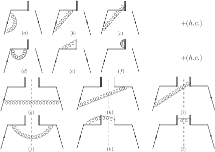
Figure 1: Complete set of the one-loop diagrams corresponding to the gauge-invariant quark TMD PDF without soft-term contributions.

Next, we evaluate the gauge field, the source of which is a charged pointlike particle (a struck quark) moving with the quasi-constant four-velocity $v_{\mu}$ along the straight line $v_{\mu}\tau$. The corresponding “classical” current then is

$$J_{\mu}(y)=g\int\!dy^{\prime}_{\mu}\ \delta^{(4)}(y-y^{\prime})\ ,\quad y^{\prime}_{\mu}=v_{\mu}\ \tau\ .$$ (8)

The velocity changes its direction only at the origin, where the collision with the hard photon takes place and the quark deviates from its initial “trajectory”. The gauge field defined by such a current then reads

$$A_{\rm LC}^{\mu}(\xi)=\int\!d^{4}y\ {\cal D}^{\mu\nu}_{\rm LC}(\xi-y)J_{\nu}(y)\ \ ,$$ (9)

where ${\cal D}^{\mu\nu}_{\rm LC}$ is the free gluon propagator in the lightcone gauge. This gauge field is exactly what forms the longitudinal gauge link[7]. We assume that the velocity of the struck quark is parallel to the “plus”- and the “minus”- lightcone vectors $n^{\pm}$ before and after the hard collision, respectively:

$$J_{\mu}(y) = g\left[n^{+}_{\mu}\int_{-\infty}^{0}\!d\tau\ \delta^{(4)}(y-n^{+}\tau)+n^{-}_{\mu}\int_{0}^{\infty}\!d\tau\ \delta^{(4)}(y-n^{+}\tau)\right]$$ (10)

$$= g\ \delta^{(2)}(\mbox{\boldmath$y$}_{\perp})\left[n^{+}_{\mu}\delta(y^{-})\int\!\frac{dq^{-}}{2\pi}\frac{{\rm e}^{-iq^{-}y^{+}}}{q^{-}+i0}-n^{-}_{\mu}\delta(y^{+})\int\!\frac{dq^{+}}{2\pi}\frac{{\rm e}^{-iq^{+}y^{-}}}{q^{+}-i0}\right]\ .$$

Then, one has

$$A_{\rm LC}^{\mu}(\xi)=-g\ n_{\nu}^{+}\int\!\frac{d^{4}q}{2(2\pi)^{4}}\ {{\rm e}^{-iq\cdot\xi}}\ \tilde{\cal D}^{\mu\nu}_{\rm LC}(q)\int\!dy^{+}dy^{-}d^{2}y_{\perp}{{\rm e}^{iq\cdot y}}\delta(y^{-})\delta^{(2)}(\mbox{\boldmath$y$}_{\perp})\ ,$$ (11)

where the free gluon propagator in the lightcone gauge $A^{+}=(A\cdot n^{-})=0$ reads

$${\cal D}^{\mu\nu}_{\rm LC}(z)=\!\int\!\frac{d^{4}q}{(2\pi)^{4}}\ {{\rm e}^{-iq\cdot z}}\tilde{\cal D}^{\mu\nu}(q)=-\!\int\!\frac{d^{4}q}{(2\pi)^{4}}\ \frac{{\rm e}^{-iq\cdot z}}{q^{2}+i0}\left(g^{\mu\nu}-\frac{q^{\mu}(n^{-})^{\nu}+q^{\nu}(n^{-})^{\mu}}{[q^{+}]_{\eta}}\right)$$ (12)

and the pole prescription $[q^{+}]_{\eta}$ has yet to be defined. We neglect the quark and gluon masses, since we are mainly interested in the UV and rapidity singularities.

After the integration over the variable $y$, we get

$$A_{\rm LC}^{\mu}(\xi)=-g\ n_{\nu}^{+}\int\!\frac{d^{4}q}{2(2\pi)^{4}}\ {{\rm e}^{-iq\cdot\xi}}\ \frac{\delta(q^{-})}{q^{2}+i0}\ \left(g^{\mu\nu}-\frac{q^{\mu}(n^{-})^{\nu}+q^{\nu}(n^{-})^{\mu}}{[q^{+}]_{\eta}}\right)\ .$$ (13)

Now we are able to calculate the plus-component of the gauge field (13) $A^{+}=(A\cdot n^{-})$:

$$A_{\rm LC}^{\mu}=-\frac{1}{2}g\ \int\!\frac{d^{4}q}{(2\pi)^{4}}\ {{\rm e}^{-iq\cdot\xi}}\ \frac{\delta(q^{-})}{q^{2}+i0}\left[n^{+\mu}-\frac{q^{\mu}}{[q^{+}]_{\eta}}\right]\ .$$ (14)

The first integral is trivial and yields (using dimensional regularization $\omega=4-2\epsilon$ for the integration over transverse degrees of freedom)

$$\int\!\frac{d^{\omega}q}{(2\pi)^{\omega}}\ {{\rm e}^{-iq\cdot\xi}}\frac{\delta(q^{-})}{q^{2}+i0}=\frac{1}{2\pi}\delta(\xi^{-})\ \int\!\frac{d^{\omega-2}q}{(2\pi)^{\omega-2}}\ \frac{{\rm e}^{i\bm{q}_{\perp}\cdot\bm{\xi}_{\perp}}}{-\mbox{\boldmath$q$}_{\perp}^{2}+i0}\ .$$ (15)

To perform the $\eta$-dependent integral, we observe that

$$\int\!\frac{d^{\omega}q}{(2\pi)^{\omega}}\ \frac{{\rm e}^{-iq\cdot\xi}}{q^{2}+i0}\ \frac{q^{+}}{[q^{+}]_{\eta}}\ \delta(q^{-})=i\frac{\partial}{\partial\xi^{-}}\ \int\!\frac{d^{\omega}q}{(2\pi)^{\omega}}\ \frac{{\rm e}^{-iq\cdot\xi}}{q^{2}+i0}\frac{\delta(q^{-})}{[q^{+}]_{\eta}}\ \ .$$ (16)

Making use of $\delta(q^{-})$ in Eq. (16), we separate out the transverse part

$$\int\!\frac{d^{\omega}q}{(2\pi)^{\omega}}\ \frac{{\rm e}^{-iq\cdot\xi}}{q^{2}+i0}\ \frac{1}{[q^{+}]_{\eta}}\ \delta(q^{-})=\frac{1}{2\pi}\ \int\!\frac{dq^{+}}{2\pi}\ \frac{{\rm e}^{-iq^{+}\xi^{-}}}{[q^{+}]_{\eta}}\ \int\!\frac{d^{\omega-2}q}{(2\pi)^{\omega-2}}\ \frac{{\rm e}^{i\bm{q}_{\perp}\cdot\bm{\xi}_{\perp}}}{-\mbox{\boldmath$q$}_{\perp}^{2}+i0}\ .$$ (17)

Consider now the longitudinal integral which we define as

$$\int\!\frac{dq^{+}}{2\pi}\ \frac{{\rm e}^{-iq^{+}\xi^{-}}}{[q^{+}]_{\eta}}=\lim_{\eta\to 0}\ \int\!\frac{dq^{+}}{2\pi}\ \frac{{\rm e}^{-iq^{+}\xi^{-}}}{q^{+}\pm i\eta}\ ,$$ (18)

where $\pm$ corresponds, respectively, to the retarded and advanced prescription, while the principal-value prescription can be obtained by symmetrization. Integral (18) can be evaluated using the residue theorem to read

$$\int\!\frac{dq^{+}}{2\pi}\ \frac{{\rm e}^{-iq^{+}\xi^{-}}}{q^{+}\pm i\eta}=\mp i\theta(\pm\xi^{-}){\rm e}^{\mp\xi^{-}\eta}\ ,\quad\theta(z)=\left\{{1\ ,\ z>0\atop 0\ ,\ z<0}\right.\ .$$ (19)

Taking the derivative with respect to $\xi^{-}$ and employing Eq. (16), we find in the limit $\eta\to 0$ the expression

$$\lim_{\eta\to 0}i\frac{\partial}{\partial\xi^{-}}\ \int\!\frac{d^{\omega}q}{(2\pi)^{\omega}}\ \frac{{\rm e}^{-iq\xi}}{q^{2}+i0}\frac{\delta(q^{-})}{[q^{+}]_{\eta}}=\frac{1}{2\pi}\ \delta(\xi^{-})\int\!\frac{d^{\omega-2}q}{(2\pi)^{\omega-2}}\ \frac{{\rm e}^{i\bm{q}_{\perp}\cdot\bm{\xi}_{\perp}}}{-\mbox{\boldmath$q$}_{\perp}^{2}+i0}\ .$$ (20)

Reversing the sign and adding this result to Eq. (15), we get, according to Eq. (14),

$$A^{+}=(A\cdot n^{-})=0\ .$$ (21)

The “minus”-component of the gauge field

$$A^{-}=(A^{\mu}\cdot n^{+}_{\mu})\sim n^{+}_{\mu}\left((n^{+})^{\mu}-\frac{q^{\mu}+q^{-}(n^{-})^{\mu}}{[q^{+}]}\right)=0-\frac{2q^{-}}{[q^{+}]}$$ (22)

vanishes as well after carrying out the integration over $q^{-}$ in Eq. (13) by virtue of $\delta(q^{-})$, i.e., $A^{-}=0$.

This suffices to show that the use of the $\eta$-dependent pole prescription in the gluon propagator is consistent with the lightcone gauge $A^{+}=0$, while for a further discussion we refer to Refs. Col11,CDL84. A formal proof of a similar statement concerning the Mandelstam-Leibbrandt pole prescription will be presented separately.

3 Lightcone TMD: One-loop effects

In the previous section, we have shown that in the lightcone gauge with $\eta$-dependent pole prescriptions for the gluon propagator, the longitudinal (lightlike) gauge links are equal to unity: $\exp[-ig\int\!dz^{-}A^{+}]=1$. Therefore, the diagrams Fig. 1 $(b,d,e,f,h,j,k)$ (and their Hermitian conjugate parts—if any) give zero contributions in the lightcone gauge, despite the opposite claims by Collins in Ref. Col11. Moreover, we give below a formal justification of our statements by demonstrating the gauge invariance of our framework.

In the lightcone gauge, the $\eta$-dependent contribution of diagram $1(a)$ is

$${\Sigma}^{(a)}[{\rm A}_{\rm n}]=-\frac{\alpha_{s}}{\pi}C_{\rm F}\ \Gamma(\epsilon)\ \left[4\pi\frac{\mu^{2}}{-p^{2}}\right]^{\epsilon}\ \delta(1-x)\delta^{(2)}(\bm{k}_{\perp})\ \int_{0}^{1}\!dx\frac{(1-x)^{1-\epsilon}}{x^{\epsilon}[x]_{\eta}}\ .$$ (23)

In a covariant gauge (definition ${\rm C}_{\rm n}$), the counterpart of this contribution stems from the vertex diagram $1(b)$ and reads

$$\Sigma^{(c)}[{\rm C}_{\rm n}]=-\frac{\alpha_{s}}{\pi}C_{\rm F}\Gamma(\epsilon)\left[4\pi\frac{\mu^{2}}{-p^{2}}\right]^{\epsilon}\ \delta(1-x)\delta^{(2)}(\bm{k}_{\perp})\ \int_{0}^{1}\!dx\ \frac{x^{1-\epsilon}}{(1-x)^{1+\epsilon}}\ .$$ (24)

By a trivial change of variables and by using the $\eta$-regularization, the singular integral above can be written as

$${\Sigma}^{(c)}[{\rm C}_{\rm n}]=-\frac{\alpha_{s}}{\pi}C_{\rm F}\ \Gamma(\epsilon)\left[4\pi\frac{\mu^{2}}{-p^{2}}\right]^{\epsilon}\delta(1-x)\delta^{(2)}(\bm{k}_{\perp})\int_{0}^{1}\!dx\frac{(1-x)^{1-\epsilon}}{x^{\epsilon}(x\pm i\eta)}={\Sigma}^{(a)}[{\rm A}_{\rm n}]\ .$$ (25)

This is an interesting result and supports the validity of the operator definition of the TMD with the lightlike longitudinal gauge links, justifying its gauge invariance at the one-loop level. Analogous results have been obtained recently within the framework of soft collinear effective theory (SCET)[23, 24, 25]. Similar problems have been addressed and resolved long ago in Ref. Ste83.

Therefore, whatever gauge is adopted, the one-loop corrections to the “unsubtracted” definition (3) give rise to pathological overlapping divergences that comprise UV and rapidity poles simultaneously ${\sim\frac{1}{\varepsilon}\ \ln\eta}$. This jeopardizes the renormalizability of TMDs and calls for a certain generalized renormalization procedure to augment the insufficient dimensional regularization. In our works[19], we worked out such a procedure that enabled us to obtain a well-defined and fully gauge-invariant TMD PDF, free of undesirable divergences. This TMD PDF has calculable renormalization-group properties and obeys an evolution equation with respect to rapidity in the impact parameter space. Moreover, the one-loop analysis of the UV anomalous dimension of the “unsubtracted” TMD PDF in (3) with the $\eta$-dependent pole prescription in the lightcone gauge shows that the overlapping singularities produces a correction to the anomalous dimension that can be identified at this order with the well-known cusp anomalous dimension[27]. The upshot of this discussion is that in order to renormalize the “naive” TMD PDF, given by (3), one has to introduce an additional renormalization factor, which depends on $\bar{\eta}=\eta/p^{+}$ and can be written as the vacuum average of the gauge links evaluated along a special contour with an obstruction (cusp)—see Ref. CKS10,CS_all for more details:

$$Z_{\eta}^{-1}=\left\langle 0\left|{\cal P}\exp\Bigg{[}ig\int_{\chi}d\zeta^{\mu}\ t^{a}A^{a}_{\mu}(\zeta)\Bigg{]}\right|0\right\rangle\ .$$ (26)

However, the overlapping singularities are not the only ones that have to be removed from the proper definition of the TMD. The one-loop corrections to the soft factor itself give rise to another type of unphysical divergences. For instance, in the lightcone gauge, the self-energy contribution of the soft factor still contains an uncanceled singularity of the term

$$\Sigma_{\rm soft}[{\rm A}_{\rm n}]=ig^{2}\mu^{2\epsilon}C_{\rm F}2p^{+}\ \int\!\frac{d^{\omega}q}{(2\pi)^{\omega}}\frac{1}{q^{2}(q^{-}\cdot p^{+}-i0)[q^{+}]_{\eta}}\ ,$$ (27)

which appears to be rapidity-independent[19]. This calls for an additional subtraction of this self-energy part that is presented graphically in Fig. 2. This subtraction does not affect the rapidity evolution equations and does not break the factorization structure (1). In fact, it has an intuitively clear physical interpretation: it serves to remove unobservable contributions due to the self-energy of the infinite lightlike gauge links that are mere artifacts of the unobservable background.

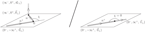
Figure 2: Subtraction of the infinite self-energy contribution of the lightlike gauge links in the soft factor.

The definition of the ${\rm A}_{\rm n}$ TMD PDF, which embodies the above requirements, reads[19]

$${\cal F}_{\rm i/h}^{[{\rm A}_{\rm n}]}\left(x,{\mathbf{k}}_{\perp};\mu,\eta\right)=\frac{1}{2}\int\frac{d\xi^{-}d^{2}\bm{\xi}_{\perp}}{2\pi(2\pi)^{2}}{\rm e}^{-ik^{+}\cdot\xi^{-}+i\bm{k}_{\perp}\bm{\xi}_{\perp}}\cdot$$

$$\times\left\langle h|\bar{\psi}_{i}(\xi^{-},\bm{\xi}_{\perp})[\xi^{-},\bm{\xi}_{\perp};\infty^{-},\bm{\xi}_{\perp}]_{n}^{\dagger}[\infty^{-},\bm{\xi}_{\perp};\infty^{-},\bm{\infty}_{\perp}]_{\mbox{\boldmath$l$}}^{\dagger}\right.\ \gamma^{+}\cdot$$

$$\left.\times[\infty^{-},\bm{\infty}_{\perp};\infty^{-},\mathbf{0}_{\perp}]_{\mbox{\boldmath$l$}}[\infty^{-},\mathbf{0}_{\perp};0^{-},\mathbf{0}_{\perp}]_{n}\psi_{i}(0^{-},\mathbf{0}_{\perp})|h\right\rangle\cdot R^{-1}\ ,$$ (28)

with the soft factor

$$R^{-1}(\mu,\eta)=$$

$$\frac{\langle 0|\ {\cal P}\exp\Big{[}ig\int_{\mathcal{C}_{\rm cusp}}\!d\zeta^{\mu}\ {\cal A}^{\mu}(\zeta)\Big{]}\cdot{\cal P}^{-1}\exp\Big{[}-ig\int_{\mathcal{C^{\prime}}_{\rm cusp}}\!d\zeta^{\mu}\ {\cal A}^{\mu}(\xi+\zeta)\Big{]}{|0\rangle}}{\langle 0|\ {\cal P}\exp\Big{[}ig\int_{\mathcal{C}_{\rm smooth}}\!d\zeta^{\mu}\ {\cal A}^{\mu}(\zeta)\Big{]}\cdot{\cal P}^{-1}\exp\Big{[}-ig\int_{\mathcal{C^{\prime}}_{\rm smooth}}\!d\zeta^{\mu}\ {\cal A}^{\mu}(\xi+\zeta)\Big{]}|0\rangle}\ ,$$

where ${\cal A}\equiv t^{a}A^{a}$ and the contours for the soft factor are displayed in Fig. 2.

4 Light-cone TMD: Evolution equations

After subtracting the soft factor, the operator definition (28) is multiplicatively renormalizable and obeys the following one-loop evolution equation with respect to the UV scale $\mu$:

$$\mu\frac{d}{d\mu}\ {\cal F}^{[{\rm A}_{\rm n}]}\left(x,{\mathbf{k}}_{\perp};\mu,\eta\right)=(\gamma_{\rm LC}+O(\alpha_{s}^{2}))\ {\cal F}^{[{\rm A}_{\rm n}]}\left(x,{\mathbf{k}}_{\perp};\mu,\eta\right)\ ,$$ (29)

where $\gamma_{\rm LC}=\frac{4\alpha_{s}}{3\pi}C_{\rm F}$ is the anomalous dimension of the bilocal quark operator in the lightcone gauge. It is interesting to note that, in the lightcone gauge with the Mandelstam-Leibbrandt prescription, the “unsubtracted” TMD (3) has an anomalous dimension that is free of any undesirable contributions and reads

$$\mu\frac{d}{d\mu}\ \left[{\cal F}_{\rm unsubtr.}^{[{\rm A}_{\rm n}^{\rm ML}]}\cdot R_{n}^{-1}\right]=\mu\frac{d}{d\mu}\ {\cal F}_{\rm unsubtr.}^{[{\rm A}_{\rm n}^{\rm ML}]}$$

$$=(\gamma_{\rm LC}+O(\alpha_{s}^{2}))\ \left[{\cal F}_{\rm unsubtr.}^{[{\rm A}_{\rm n}^{\rm ML}]}\cdot R_{n}^{-1}\right]=(\gamma_{\rm LC}+O(\alpha_{s}^{2}))\ {\cal F}_{\rm unsubtr.}^{[{\rm A}_{\rm n}^{\rm ML}]}\ .$$ (30)

In the one-loop approximation, these results are in agreement with those given in Ref. AR11.

In order to study the rapidity evolution, we have to concentrate on the specific TMD singularities which only depend on the additional rapidity parameter $\eta$, but else do not violate the renormalizability of the TMDs. These singular terms have to be resummed by means of an equation of the Collins–Soper type[4, 5]. Our framework indeed allows the development of such a resummation procedure of the rapidity divergences as we now show.

To this end, recall that the $\eta$-dependent part (23) of the quark self-energy diagram corresponding to Fig. 1$(a)$ has the form

$${\Sigma}^{(a)}[{\rm A}_{\rm n}] = -\frac{\alpha_{s}}{\pi}C_{\rm F}\ \Gamma(\epsilon)\ \left[4\pi\frac{\mu^{2}}{-p^{2}}\right]^{\epsilon}\ \delta(1-x)\delta^{(2)}({\boldmath k_{\perp}})\$$ (31)

$$\times \frac{1}{p^{+}}\left[-1-\ln\frac{\pm i\eta}{p^{+}}-\epsilon\left(2-\frac{\pi^{2}}{3}-\frac{1}{2}\ln^{2}\frac{\pm i\eta}{p^{+}}\right)+O(\epsilon^{2})\right]\ ,$$

where the quadratic term $\sim\ln^{2}\eta$ is responsible for the “rapidity” evolution. The linear terms stem from the remaining virtual and real graphs of the “unsubtracted” TMD and the soft factor.

In order to confront our framework with the Collins-Soper rapidity evolution approach, we make use of the impact representation of the TMD

$${\cal F}\left(x,{\mathbf{b}}_{\perp};\mu,\eta\right)=\int\!d^{2}{\mathbf{k}_{\perp}}\ {\rm e}^{i\bm{b}_{\perp}\cdot\bm{k}_{\perp}}\ {\cal F}\left(x,{\mathbf{k}}_{\perp};\mu,\eta\right)\ .$$ (32)

Then, the Collins-Soper rapidity evolution equation (which holds for the off-the-light-cone A_v-TMD and C_v-TMD) becomes

$$\zeta\frac{\partial}{\partial\zeta}\ {\cal F}_{[{\rm A,C}_{\rm v}]}\left(x,{\mathbf{k}}_{\perp};\mu,\zeta\right)=\left[K_{\rm v}(\mu,b_{\perp})+G_{\rm v}(\mu,\zeta)\right]\ {\cal F}_{[{\rm A,C}_{\rm v}]}\left(x,{\mathbf{k}}_{\perp};\mu,\zeta\right)\ ,$$ (33)

where the functions $K$ and $G$ have the following renormalization-group properties:

$$\mu\frac{d}{d\mu}K_{\rm v}=-\mu\frac{d}{d\mu}G_{\rm v}=\gamma_{\rm cusp}\ .$$ (34)

In our approach, the analogue of the Collins-Soper rapidity cutoff is given by the new variable $\theta\equiv(p\cdot n)/\eta$. Therefore, the corresponding evolution equation takes the form

$$\theta\frac{\partial}{\partial\theta}\ {\cal F}_{[{\rm A}_{\rm n}]}\left(x,{\mathbf{k}}_{\perp};\mu,\theta\right)=\left[K_{\rm n}(\mu,\mbox{\boldmath$b$}_{\perp})+G_{\rm n}(\mu,\theta)\right]\ {\cal F}_{[{\rm A}_{\rm n}]}\left(x,{\mathbf{k}}_{\perp};\mu,\theta\right)\ ,$$ (35)

noting that the limit $\eta\to 0$ corresponds to the limit $\zeta\to\infty$ in the Collins-Soper approach. Here the sum $K_{\rm n}+G_{\rm n}$ for the A_n-TMD can be evaluated perturbatively in the small-$\mbox{\boldmath$b$}_{\perp}$ region. The relation (34) for the A_n-TMD has been verified at the one-loop level in our previous works[19]. Explicit results for the rapidity evolution kernel $\left[K_{\rm n}(\mu,\mbox{\boldmath$b$}_{\perp})+G_{\rm n}(\mu,\theta)\right]$ will be reported in the future.

The bottom line is: the generalized definition of the TMD PDF (28) allows one to derive its renormalization-group evolution with respect to the UV scale $\mu$ and to resum the large rapidity logarithms by means of the evolution equation (35), formally akin to that in the Collins-Soper procedure, designed for off-the-light-cone quantities.

5 Conclusions and discussion

To conclude, we have shown that the completely gauge-invariant operator definition of the transverse-momentum-dependent parton densities, which makes use of longitudinal lightlike gauge links and also of appropriate transverse gauge links at lightcone infinity, can be consistently formulated beyond the tree-level approximation—at least in the one-loop order. The advantages of the presented approach are:

• In the lightcone axial gauge, the longitudinal gauge links cancel, while the transverse gauge links can be eliminated by proper boundary conditions for the gauge fields at lightcone infinity. This provides a natural framework for QCD factorization schemes, where the use of covariant gauges and not purely lightlike gauge links is not convenient.

• A direct relationship between the (unintegrated) TMDs and the (integrated) collinear PDFs can be established by straightforward $\mbox{\boldmath$k$}_{\perp}$-integration. One ultimately gets the well-known collinear and gauge-invariant PDF that fulfills the DGLAP evolution equation (in the one-loop order).

• The transverse gauge links at lightcone infinity (supplemented by appropriate boundary conditions) accumulate information about the initial- and/or final-state interactions in the axial gauges, in which the longitudinal gauge links disappear. The transverse gauge links naturally shrink to harmless constants after performing the $\mbox{\boldmath$k$}_{\perp}$-integration without causing a breakdown of the standard structure of the longitudinal gauge links in the collinear PDF, while in the case of the off-the-light-cone definitions this is, at least, not obvious.

• Moreover, the transverse gauge links are responsible for $T$-odd effects in the lightcone gauge that makes it possible to apply this framework to the study of phenomenologically important quantities, such as the Sivers, Boer-Mulders, Collins functions, etc.

• A complete proof of the QCD factorization within the presented scheme—in particular, the evaluation of the hard part in the lightcone gauge and the explicit demonstration of the independence of the full structure functions of unphysical scales is still lacking and will be treated in the future.

References

• [1] D. E. Soper, Phys. Rev.  D 15, 1141 (1977); Phys. Rev. Lett. 43, 1847 (1979).
• [2] J. C. Collins, Phys. Rev. Lett.  42, 291 (1979).
• [3] J. P. Ralston and D. E. Soper, Nucl. Phys.  B, 109 152 (1979).
• [4] J. C. Collins and D. E. Soper, Nucl. Phys. B 193, 381 (1981); Nucl. Phys. B 213, 545 (1983) Erratum.
• [5] J. C. Collins and D. E. Soper, Nucl. Phys. B 194, 445 (1982).
• [6] J. C. Collins, D. E. Soper and G. F. Sterman, Nucl. Phys.  B 250, 199 (1985).
• [7] A.V. Belitsky, X. Ji and F. Yuan, Nucl. Phys. B 656, 165 (2003).
• [8] D. Boer, P.J. Mulders and F. Pijlman, Nucl. Phys. B 667, 201 (2003).
• [9] F. Hautmann, Phys. Lett. B 655, 26 (2007).
• [10] J. C. Collins and A. Metz, Phys. Rev. Lett.  93, 252001 (2004).
• [11] I. O. Cherednikov, A. I. Karanikas and N. G. Stefanis, Nucl. Phys.  B 840, 379 (2010).
• [12] B. U. Musch, P. Hägler, A. Schäfer, D. B. Renner and J. W. Negele LHPC (Lattice Hadron Physics Collaboration), PoS LC2008, 053 (2008).
• [13] J. C. Collins, Acta Phys. Pol. B 34, 3103 (2003).
• [14] A. V. Belitsky, A. V. Radyushkin, Phys. Rept.  418, 1 (2005).
• [15] J. C. Collins, T. C. Rogers and A. M. Stasto, Phys. Rev. D, 085009 77 (2008).
• [16] J. Collins, PoS LC2008, 028 (2008).
• [17] S. M. Aybat and T. C. Rogers, Phys. Rev.  D 83, 114042 (2011).
• [18] J. Collins, arXiv:1107.4123 [hep-ph].
• [19] I. O. Cherednikov and N. G. Stefanis, Phys. Rev. D 77, 094001 (2008); Nucl. Phys. B 802, 146 (2008); Phys. Rev. D 80, 054008 (2009); N. G. Stefanis and I. O. Cherednikov, Mod. Phys. Lett. A 24, 2913 (2009).
• [20] I. O. Cherednikov, arXiv:1102.0892 [hep-ph].
• [21] N. G. Stefanis, I. O. Cherednikov and A. I. Karanikas, PoS LC2010, 053 (2010).
• [22] D. M. Capper, J. J. Dulwich and M. J. Litvak, Nucl. Phys.  B 241, 463 (1984).
• [23] A. Idilbi and I. Scimemi, Phys. Lett.  B 695, 463 (2011).
• [24] M. García-Echevarría, A. Idilbi and I. Scimemi, Phys. Rev. D 84, 011502(R) (2011).
• [25] Y. Li, S. Mantry and F. Petriello, arXiv:1105.5171 [hep-ph].
• [26] N. G. Stefanis, Nuovo Cim. A 83, 205 (1984).
• [27] G. P. Korchemsky and A. V. Radyushkin, Nucl. Phys. B 283, 342 (1987).