All good things come in threes - Three beads learn to swim with lattice Boltzmann and a rigid body solver

Abstract

We simulate the self-propulsion of devices in a fluid in the regime of low Reynolds numbers. Each device consists of three bodies (spheres or capsules) connected with two damped harmonic springs. Sinusoidal driving forces compress the springs which are resolved within a rigid body physics engine. The latter is consistently coupled to a 3D lattice Boltzmann framework for the fluid dynamics. In simulations of three-sphere devices, we find that the propulsion velocity agrees well with theoretical predictions. In simulations where some or all spheres are replaced by capsules, we find that the asymmetry of the design strongly affects the propelling efficiency.

1 Introduction

Engineered micro-devices, developed in such a way that they are able to move alone through a fluid and, simultaneously, emit a signal, can be of crucial use in various fields of science. A few engineered self-propulsive devices have been developed over the last decade. In one approach, the device consisted of magnetically actuated superparamagnetic particles linked together by DNA double strands [8]. In another approach, miniature semiconductor diodes floating in water were used. When powered by an external alternating electric field, the voltage induced between the diode electrodes changed, which resulted in particle-localized electro-osmotic flow. In the latter case, the devices could respond and emit light, thus providing a signal that could be used as a carrier [5]. A third example is a swimmer based on the creation of a traveling wave along a piezoelectric layered beam divided into several segments with a voltage with the same frequency but different phases and amplitudes applied to each segment [21].

Propulsion through a fluid induces the flow of the surrounding fluid, which in turn affects the propulsion of the device. Most generally the fluid motion is described by the Navier-Stokes equation

$$\frac{\partial\vec{u}}{\partial t}+(\vec{u}\cdot\nabla)\vec{u}=-\frac{1}{\rho}\nabla p+\frac{\mu}{\rho}\nabla^{2}\vec{u}+\vec{f}.$$ (1)

Here $\vec{u}$ is the velocity, $\rho$ is the density, $p$ is the pressure, $\mu$ is the dynamic viscosity of the fluid, and $\vec{f}$ is the applied force in the fluid. The first term on the left hand side describes the acceleration of the fluid, whereas the second term accounts for non-linear inertial effects that may give rise to effects such as turbulence. On the right hand side the first term is the driving pressure gradient, while the second term takes into account the viscous dissipation.

In the case of low Reynolds numbers, the inertia terms on the left side of equation (1) can be dropped and one is left with

$$0=-\frac{1}{\rho}\nabla p+\frac{\mu}{\rho}\nabla^{2}\vec{u}+\vec{f},$$ (2)

which together with the incompressibility equation $\nabla\cdot\vec{u}=0$ describes the so-called Stokes flow. The main characteristics of the Stokes flow emerge from the domination of viscous forces. Consequently, the flow is always laminar (no turbulence or vortex shedding) and characterized by a small momentum. Since the flow is proportional to the forces applied, linear superposition of solutions is valid. Furthermore, the Stokes flow is instantaneous, which means that the time-development is given solely by the effects of the boundaries. Finally, there is no coasting, and the flow is time-reversible, which has important implications for swimming strategies at low Reynolds numbers [36].

The propulsion strategy in this regime must involve a non-time-reversible motion, thus involving more than one degree of freedom [32]. Such a requirement is not limiting if a large number of degrees of freedom is available. However, if one tries to design a self-propelled device (e.g. a swimmer) with only a few degrees of freedom, a balance between simplicity and functionality has to be found.

A number of analytic and numerical studies have been performed to understand the behavior of a single or a couple of swimmers under various conditions [13, 22]. However, most of these types of approaches are limited to simple geometries of swimmers and fail when numerous swimmers are involved leading to a collective behavior. In addition to the effective treatment of many body interactions, the regimes in which inertia starts to play a role, as well as the problem of motion in confined geometry or transport in turbulent flow, are inaccessible. In these circumstances extensive simulations become essential, but difficult to perform efficiently [31, 38].

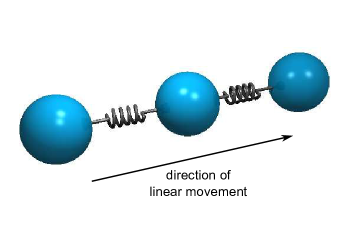
Figure 1: A three-sphere swimming device with two translational degrees of freedom.

In order to meet these challenges, we augmented our already existing massively parallel lattice Boltzmann simulation framework waLBerla, widely applicable Lattice Boltzmann solver from Erlangen [10], with swimmers. The motion of the latter is included into waLBerla by coupling it with the $\mathpzc{pe}$ rigid multibody physics engine, a framework for the simulation of rigid, fully resolved bodies of arbitrary shape [16]. This allows us to resolve both, the driven motion of a swimmer within the fluid, and the induced motion of the fluid in a consistent manner. For the swimming device we choose the simplest possible design, consisting of three rigid bodies connected with two springs (Figure 1). This design has been studied extensively in the three spheres geometry by analytical methods [12].

This paper starts with the elucidation of the background of the numerical methods, which form the basis of our simulation, in Section 2. Here, the lattice Boltzmann method (LBM) of the waLBerla framework, the mechanics of the $\mathpzc{pe}$ framework and, finally, the coupling of both with special focus on the swimmers are briefly explained. In Section 3, our new implementation approach for the integration of the swimmers is considered in detail, including the cycling strategy. Moreover, our design variants are presented. Afterwards, in Section 4, a quantitative validation of the simulation results of the $\mathpzc{pe}$ engine is conducted. In Section 5, validation criteria for the swimmer are defined, and asymmetric and symmetric designs are simulated and analyzed in detail to demonstrate the capability of our extension of the framework. Finally, in Section 6 a conclusion of the achieved results is given, and propositions for future work are made.

2 Numerical methods

2.1 The lattice Boltzmann method

The LBM can be used as an alternative to the classical Navier–Stokes (NS) solvers to simulate fluid flows [6, 35] The fluid is modeled as a set of imaginary, discretized particles positioned on an equidistant grid of lattice cells. Moreover, the particles are only allowed to move in fixed, pre-defined directions given by the finite set of velocity vectors, resulting from the discretization of the velocity space. Unlike other methods, which rely on the automatic generation of a body fitted mesh during the simulation, the waLBerla framework uses the LBM on the same (block-)structured mesh, even when the objects are moving. This eliminates the need for dynamic re-meshing, and hence offers a significant advantage with respect to performance.

In this study we use the common three-dimensional D3Q19 velocity phase discretization model originally developed by Qian, d’Humières and Lallemand [34] with $N=19$ particle distribution functions (PDFs) $f_{\alpha}:\Omega\times T\rightarrow[0,1)$, where $\Omega\subset\mathbb{R}^{3}$ and $T\subset\mathbb{R}^{+}_{0}$ are the spatial and the time domain, respectively.

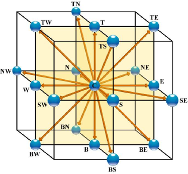
Figure 2: The D3Q19 velocity phase discretization model.

Figure 2 illustrates the 19 directions. The corresponding dimensionless discrete velocity set is denoted by $\{\vec{e}_{\alpha}|\alpha=0,\ldots,N-1\}$. This model has been shown to be both stable and efficient [26]. For the work presented in this paper, we adopt a lattice Boltzmann collision scheme proposed by Bhatnagar, Gross and Krook, called lbgk [3, 34]

$$f_{\alpha}(\vec{x}_{i}+\vec{e}_{\alpha}\Delta t,t+\Delta t)=f_{\alpha}(\vec{x}_{i},t)-\frac{1}{\tau}[f_{\alpha}(\vec{x}_{i},t)-f_{\alpha}^{(\operatorname{eq})}(\vec{x}_{i},t)]\,,$$ (3)

where $\vec{x}_{i}$ is a cell in the discretized simulation domain, $t$ is the current time step, $t+\Delta t$ is the next time step, $\tau$ is the relaxation time in units of time step $\Delta t$ (which is set to be 1 here) and $f_{\alpha}^{(\operatorname{eq})}$ represents the equilibrium distribution.

The time evolution of the distribution function, given by equation (3), is usually solved in two steps, known as the collision step and the streaming step, respectively:

$$\tilde{f}_{\alpha}(\vec{x}_{i},t)=f_{\alpha}(\vec{x}_{i},t)-\frac{1}{\tau}[f_{\alpha}(\vec{x}_{i},t)-f_{\alpha}^{(\operatorname{eq})}(\vec{x}_{i},t)]\,,$$ (4)

$$f_{\alpha}(\vec{x}_{i}+\vec{e}_{\alpha}\Delta t,t+\Delta t)=\tilde{f}_{\alpha}(\vec{x}_{i},t)\,,$$ (5)

where $\tilde{f}_{\alpha}$ denotes the post-collision state of the distribution function. The collision step is a local single-time relaxation towards equilibrium. The streaming step advects all PDFs except for $f_{0}$ to their neighboring lattice site depending on the velocity. Thus, for each time step only the information of the next neighbors is needed.

As a first-order no-slip boundary condition a simple bounce-back scheme is used, where distribution functions pointing to a neighboring wall are just reflected such that both normal and tangential velocities vanish:

$$f_{\bar{\alpha}}(\vec{x}_{f},t)=\tilde{f}_{\alpha}(\vec{x}_{f},t)\,,$$ (6)

with $\bar{\alpha}$ representing the index of the opposite direction of $\alpha$, $\vec{e}_{\bar{\alpha}}=-\vec{e}_{\alpha}$, and $\vec{x}_{f}$ explicitly denoting the fluid cell.

Due to the locality of the cell updates, the LBM can be implemented extremely efficiently (see for instance [30, 37]). For the same reason, the parallelization of LBM is comparatively straightforward [20]. It is based on a subdomain partitioning that is realized in the waLBerla framework by a patch data structure as described in Feichtinger et al. [10].

2.2 The rigid body physics engine $\mathpzc{pe}$

Simulating the dynamics of rigid bodies involves both the treatment of movement by a discretization of Newton’s equations of motion, as well as handling collisions between rigid objects. The forces involved may be external, such as gravity, or between bodies, such as springs. Furthermore, a number of velocity constraints are available through which hinges, sliders, ball joints and the like are implemented [28]. The collisions between rigid bodies are either treated directly by the application of the restitution laws in the form of a linear complementarity problem (LCP) [2] or by applying Hertzian contact mechanics (as for instance in the DEM approach) [7].

In our work, we fully resolve the geometry of the rigid bodies. In contrast to mass-point-based approaches, this for instance enables us to easily exchange the geometries of the swimmers in our simulations (see Subsection 3.2). The rigid body framework used for this is the $\mathpzc{pe}$ rigid multibody physics engine [16]. Due to its highly flexible, modular and massively parallel implementation, the framework allows for a direct selection of the time discretization scheme and collision treatment. By this it can easily be adjusted to various simulation scenarios. For instance, it has already been successfully used to simulate large-scale granular flow scenarios [17] and can be efficiently coupled for simulations of particulate flows [15] (see Subsection 2.3).

The springs of the $\mathpzc{pe}$ are modeled as damped harmonic oscillators in which the bodies are subject to the harmonic and the damping force. The first one is

$$\vec{F}_{\text{spring}}^{S_{n}}=-k\,\Delta\vec{x}^{S_{n}}\hskip 14.22636pt\text{for all springs }n,$$ (7)

where $k$ is the force constant and $\Delta\vec{x}^{S_{n}}=(\vec{x}^{B_{i}}-\vec{x}^{B_{j}})-\vec{l}_{0}$ is the deformation of the spring for $i\neq j$. The deformation is defined as the difference between the rest length $\vec{l}_{0}$ of the spring and its current length, which equals the current distance between the connected bodies $B_{i}$ and $B_{j}$, whose current positions are denoted by $\vec{x}^{B_{i}}$ and $\vec{x}^{B_{j}}$, respectively. In order to account for the dissipation in the spring, a damping force, proportional to the velocity $\Delta\vec{u}^{S_{n}}$ at which the spring is contracting is implemented as in the following

$$\vec{F}_{\text{damp}}^{S_{n}}=-\gamma\,\Delta\vec{u}^{S_{n}}\hskip 14.22636pt\text{for all springs }n.$$ (8)

Here $\gamma$ is the damping coefficient and $\Delta\vec{u}^{S_{n}}=\vec{u}^{B_{i}}-\vec{u}^{B_{j}}$ for $i\neq j$. Here, $\vec{u}^{B_{i}}$ and $\vec{u}^{B_{j}}$ are the velocities of the bodies $B_{i}$ and $B_{j}$. This damping force hence models the internal friction resulting from the deformation of the spring. Consequently, each of the two bodies $B_{i}$ and $B_{j}$ connected by a spring $S_{n}$ feels the force

$$\vec{F}_{\text{osci}}^{B_{i}} =-k\,\Delta\vec{x}^{S_{n}}-\gamma\,\Delta\vec{u}^{S_{n}},$$ (9)

$$\vec{F}_{\text{osci}}^{B_{j}} =\;\;\;k\,\Delta\vec{x}^{S_{n}}+\gamma\,\Delta\vec{u}^{S_{n}},$$ (10)

respectively.

A standard way to classify a damped harmonic oscillator is by its damping ratio

$$D=\frac{\gamma}{2\sqrt{m\,k}}.$$ (11)

If $D>1$ the system is overdamped and upon an excitation the system returns exponentially to equilibrium without oscillating. If $D\ll 1$ the system is underdamped. It will oscillate with a re-normalized frequency decreasing the amplitude to zero until the equilibrium state is reached. We choose the parameters of the springs of the swimmer in such a way that the latter regime is achieved.

Algorithm 1 Rigid Body Time Step

1:  //Collision detection

2:  for each rigid body ${B_{i}}$ do

3:     Detect all contacts k

4:     Add them to set of constraints c

5:  end for

6:  

7:  //Constraint resolution

8:  for each constraint c do

9:     Determine acting constraint forces $\vec{F}^{B_{i}}_{\text{c}}$

10:  end for

11:  

12:  //Time integration

13:  for each rigid body $B_{i}$ do

14:     Apply forces $\vec{F}^{B_{i}}_{\text{tot}}$: update position and velocity

15:  end for

Algorithm 1 gives an overview of the necessary steps within a single time step of the $\mathpzc{pe}$ framework. During each time step, collisions between rigid bodies have to be detected and resolved appropriately in order to keep rigid bodies from interpenetrating. Therefore, initially, all contacts $k$ between pairs of colliding rigid bodies are detected and added to the set of constraints $c$, which already includes the potentially existing velocity constraints. In the subsequent constraint resolution step, the acting constraining forces $\vec{F}^{B_{i}}_{\text{c}}$, including the forces of the harmonic potentials $\vec{F}^{B_{i}}_{\text{osci}}$, are determined. Moreover, the detected collisions are resolved depending on the selected collision response algorithm. It is important to note that interpenetration cannot be completely prevented due to the discrete time stepping, but small penetrations can be corrected in the collision response phase. In the final step all rigid bodies ${B_{i}}$ are moved forward in time according to Newton’s laws of motion, depending on their current velocity and the total forces $\vec{F}^{B_{i}}_{\text{tot}}$ acting at the given instance of time.

In the simulations of swimmers, the size of the time step was chosen such that rigid bodies do not interpenetrate. Another limitation on the size of the time step originates from the force constant of the harmonic oscillators and the frequency of the driving forces. In all cases the time step must be small enough to enable all bodies to respond sufficiently quickly to changes in the acting forces.

2.3 Coupling lattice Boltzmann to the $\mathpzc{pe}$ for swimmers

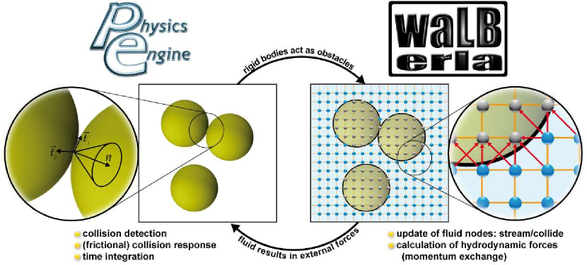
Figure 3: Illustration of the two-way coupling of waLBerla fluid solver and $\mathpzc{pe}$ rigid body dynamics solver.

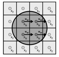
(a) Initial setup: The velocities $\vec{u}$ of the object cells $\vec{x}_{b}$ are set to the velocity $\vec{u}_{w}(\vec{x}_{b})$ of the object. In this example the object only has a translational velocity component. Fluid cells are marked with $\vec{x}_{f}$.

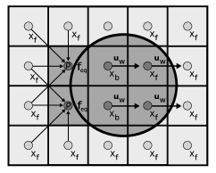
(b) Updated setup: Two fluid cells have to be transformed to object cells, and for two object cells the PDFs have to be reconstructed.

Figure 4: 2D mapping example [14].

The coupling between the lattice Boltzmann flow solver and the rigid body dynamics simulation has to be two-way: rigid bodies have to be represented as (moving) boundaries in the flow simulation, whereas the flow corresponds to hydrodynamic forces acting on the rigid bodies (Figure 3). We use an explicit coupling algorithm, shown in Algorithm 2, which we adopt for the swimmers. The additional steps are highlighted. Here, a driving force acts on the corresponding bodies according to a carefully defined protocol (see Subsection 3.3).

Algorithm 2 Coupled LBM-PE solver for the swimmers

1:  for each swimmer S do

2:     Map S to lattice grid

3:  end for

4:  

5:  for each lattice cell do

6:     Stream and collide

7:  end for

8:  

9:  for each surface cell do

10:     Add forces $\vec{F}^{B_{i}}_{\text{hydro}}$ from fluid to rigid objects ${B_{i}}$

11:  end for

12:  

13:  for each body ${B_{i}}$ of the swimmers do

14:     Add external forces $\vec{F}^{B_{i}}_{\text{dri}}$

15:  end for

16:  

17:  //Time step in the rigid body simulation (see Algorithm 1)

18:  for each rigid body $B_{i}$ do

19:     $\hskip 11.38092pt\vec{F}^{B_{i}}_{\text{tot}}=\vec{F}^{B_{i}}_{\text{hydro}}+\vec{F}^{B_{i}}_{\text{dri}}+\vec{F}^{B_{i}}_{\text{c}}$

20:  end for

The first step in the coupled algorithm is the mapping of all rigid bodies onto the lattice Boltzmann grid (see Figure 4(a) for an example). Objects are thus represented as flag fields for the flow solver. In our implementation, each lattice node with a cell center inside an object is treated as a moving boundary. For these cells, we apply the boundary condition

$$f_{\bar{\alpha}}(\vec{x}_{f},t) = \tilde{f}_{\alpha}(\vec{x}_{f},t)+6w_{\alpha}\rho_{w}(\vec{x}_{f},t)\vec{e}_{\bar{\alpha}}\cdot\vec{u}_{w}(\vec{x}_{f}+\vec{e}_{\alpha},t)\,,$$ (12)

which is a variation of the standard no-slip boundary conditions for moving walls [39]. Here $\rho_{w}(\vec{x}_{f},t)$ is the fluid density close to the wall, $w_{\alpha}$ is the weight in the LBM depending on the stencil and the direction, and the velocity $\vec{u}_{w}(\vec{x}_{f}+\vec{e}_{\alpha},t)$ of each object cell corresponds to the velocity of the object at the cell’s position at time $t$. In this way, the fluid at the surface of an object is given the same velocity as the object’s surface which depends on the rotational and the translational velocities of the object.

The final part of the first step is to account for the flag changes due to the movement of the objects. Here, two cases can occur (see Figure 4(b)): the fluid cells $\vec{x}_{f}$ can turn into object cells, resulting in a conversion of the cell to a moving boundary. In the reverse case, i.e. a boundary cell turns into a fluid cell, the missing PDFs have to be reconstructed. In our implementation, the missing PDFs are set to the equilibrium distributions $f^{(eq)}_{\alpha}(\rho,\vec{u})$, where the macroscopic velocity $\vec{u}$ is given by the velocity $\vec{u}_{w}(\vec{x}_{f})$ of the object cell, and the density $\rho$ is computed as an average of the surrounding fluid cells. Further details of this procedure have been discussed previously by us in Iglberger et al. [18]. There are more formal ways for the initialization of the missing distribution functions. One of them is described in the paper by Mei et al. [25].

During the subsequent stream and collide step, the fluid flow acts through hydrodynamic forces on the rigid objects: Fluid particles stream from their cells to neighboring cells and, in case they enter a cell occupied by a moving object, are reversed, causing a momentum exchange between the fluid and the particles. The total hydrodynamic force $\vec{F}^{B_{i}}_{\text{hydro}}$ on each object ${B_{i}}$ resulting from this momentum exchange [39] can be easily evaluated due to the kinetic origin of the LBM by

$$\vec{F}^{B_{i}}_{\text{hydro}}=\sum_{\vec{x}_{b}}\sum_{\alpha=1}^{19}\vec{e}_{\alpha}\left[2\tilde{f}_{\alpha}(\vec{x}_{f},t)+6w_{\alpha}\rho_{w}(\vec{x}_{f},t)\vec{e}_{\bar{\alpha}}\cdot\vec{u}_{w}(\vec{x}_{f}+\vec{e}_{\alpha},t)\right]\frac{\Delta x}{\Delta t}\,,$$ (13)

where $\vec{x}_{b}$ are all obstacle cells of the object that neighbor at least one fluid cell. A comparison of different approaches for the momentum exchange is given in Lorenz et al. [24].

In the third step, the driving force $\vec{F}^{B_{i}}_{\text{dri}}$, resulting from the cycling strategy, is added to the previously calculated hydrodynamic force on each body ${B_{i}}$. Together with the constraint force $\vec{F}^{B_{i}}_{\text{c}}$, this results in a total force

$$\vec{F}^{B_{i}}_{\text{tot}}=\vec{F}^{B_{i}}_{\text{hydro}}+\vec{F}^{B_{i}}_{\text{dri}}+\vec{F}^{B_{i}}_{\text{c}}$$ (14)

on each object.

The fourth and final step of the coupling algorithm consists of determining the rigid body movements of the objects due to the influence of $\vec{F}^{B_{i}}_{\text{tot}}$ in the rigid body framework. This results in a position change of the objects, which then are mapped again to the LBM grid in the next time step. A validation of this method is described in Binder et al. [4], and Iglberger et al. [18].

3 Integration of the swimming device

The modeling of a three-sphere swimmer always involves a similar physical setup. On the one hand, the connections between the objects need to be modeled. Here, stiff rods [27, 33] or springs [11] are most commonly used. On the other hand, the cycling strategy, responsible for the characteristic movement of the swimmer, needs to be defined.

3.1 Elementary design

Figure 5: A three-sphere swimming device. The three spheres have the same mass $m_{\text{sph}}$ and radius $r_{\text{sph}}$. Similarly, the two damped harmonic oscillators have identical force constant $k$, damping parameter $\gamma$, and rest length $l_{0}$.

Our elementary design (Figure 5), inspired by the analytical modeling in Golestanian and Ajdari [12], and in Felderhof [11], consists of three spheres ($B_{1},B_{2},B_{3}$) with identical radius $r_{\text{sph}}$ and mass $m_{\text{sph}}$. The connections between the three rigid objects of our swimmer are realized by two damped harmonic springs $S_{1}$ and $S_{2}$ with equal force constant $k$ and damping parameter $\gamma$. The forces are applied on the spheres along the main axis of the swimmer, in our case the z-axis, resulting in a translation of the swimmer in this direction.

In accordance with the equations (9) and (10), the different objects feel the force

$$\vec{F}_{\text{osci}}^{B_{2}} =-k\,\Delta\vec{x}^{S_{1}}-\gamma\,\Delta\vec{u}^{S_{1}},$$ (15)

$$\vec{F}_{\text{osci}}^{B_{1}} =\;\;\,k\,\left(\Delta\vec{x}^{S_{1}}+\Delta\vec{x}^{S_{2}}\right)+\gamma\,\left(\Delta\vec{u}^{S_{1}}+\Delta\vec{u}^{S_{2}}\right),$$ (16)

$$\vec{F}_{\text{osci}}^{B_{3}} =-k\,\Delta\vec{x}^{S_{2}}-\gamma\,\Delta\vec{u}^{S_{2}},$$ (17)

respectively.

Since the bodies of the swimmer do not collide with each other, the total force acting on each body $B_{i}$ of the swimmer, given in equation (14), can be rewritten as

$$\vec{F}^{B_{i}}_{\text{tot}}=\vec{F}^{B_{i}}_{\text{hydro}}+\vec{F}^{B_{i}}_{\text{dri}}+\vec{F}^{B_{i}}_{\text{osci}}.$$ (18)

3.2 Alternative designs

Since we want to investigate the effect of different geometries on the swimming behavior of our self-propelled device, we will replace the spheres of the elementary three-sphere swimmer design by capsules. For example, Figure 6 depicts the characteristic parameters of a three-capsule swimming device. The comparably smooth edges of a capsule, and thus its resulting smooth behavior in a fluid, substantiate our choice of this particular geometry. Figure 7 shows our assembly variants.

Figure 6: A three-capsule swimming device. The three capsules have the same mass $m_{\text{cap}}$, length $l_{\text{cap}}$ and radius $r_{\text{cap}}$. Similarly, the two damped harmonic oscillators have identical force constant $k$, damping parameter $\gamma$, and rest length $l_{0}$.

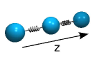
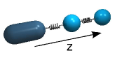
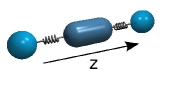
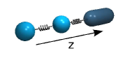
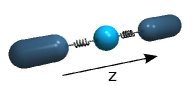
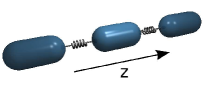
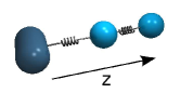
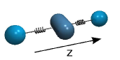
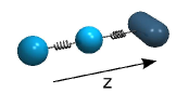
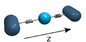
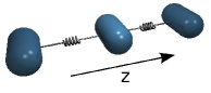
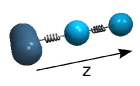
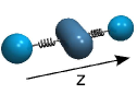
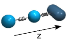
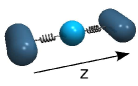
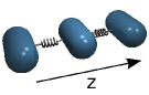
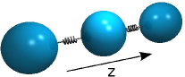
Figure 7: Design options 7–7 of our swimming device. The capsules in the designs 7–7 are rotated by $\pi/2$. Further, the spheres in design 7 have larger radii, equal to the lengths of the capsules in 7 and 7.

3.3 Cycling strategy

Purcell’s Scallop theorem [32] necessitates the motion of a swimmer to be non-time-reversible at low Reynolds numbers. Additionally, the total applied force on a swimmer should vanish over one cycle, which means that the displacement of the center of mass of a swimmer over one cycle should be zero in the absence of a fluid.

In contrast to the common approach of imposing known velocities on the constituent bodies of a swimmer, used, e.g., by Earl et al. [9] and Najafi and Golestanian [27], our driving protocol imposes known forces on the objects. These forces, only applied along the main axis of the swimmer on the center of mass of each body, are given by

$${\left(\vec{F}_{\text{dri}}^{B_{2}}\right)}_{z} =-a\cdot\text{sin}\left(\omega t\right)=-a\cdot\text{sin}\left(\frac{2\pi t}{T}\right),$$ (19)

$${\left(\vec{F}_{\text{dri}}^{B_{3}}\right)}_{z} =\;\;\;a\cdot\text{sin}\left(\frac{2\pi(t+\varphi)}{T}\right),$$ (20)

$${\left(\vec{F}_{\text{dri}}^{B_{1}}\right)}_{z} =-\left({\left(\vec{F}_{\text{dri}}^{B_{2}}\right)}_{z}+{\left(\vec{F}_{\text{dri}}^{B_{3}}\right)}_{z}\right).$$ (21)

Here $a$ is the amplitude, $\omega$ is the driving frequency, $T$ is the oscillation period, and $\varphi$ is the phase shift, kept constant at a value of $\varphi=T/4$. In equation (21), we apply the negative sum of the forces of the two outer bodies $B_{2}$ and $B_{3}$ on the middle body $B_{1}$ in order to ensure that the net driving force acting on the system at each instant of time is zero. Figure 8 illustrates these forces.

Figure 8: Fragments of the z-components of the driving forces on all three bodies.

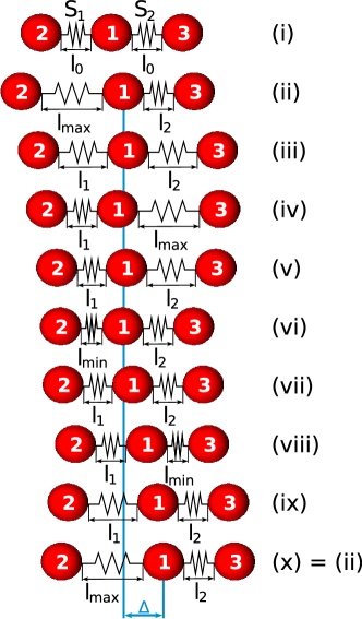
(a) Theoretical positions prescribed by the cycling strategy.

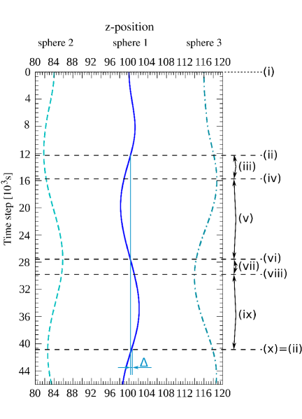
(b) Position plot from the simulation. The z-positions are given in lattice cells.

Figure 9: Cycling strategy of the non-time-reversible motion, exemplified on the three-sphere swimmer. For both damped harmonic potentials, $l_{\text{min}}$ is the minimum length of one arm, $l_{0}$ is the rest length, and $l_{\text{max}}$ is the maximal extended armlength. $\Delta$ is the distance covered by the swimmer after one cycle.

Applying this force protocol to our swimmer, we end up with our cycling strategy illustrated in Figure 9. Starting from the rest position, we have to delay the force on body $B_{3}$ by a fourth of the pulse length. Step (i) depicts the initial position of our swimming device. The two “arms ”, i.e. the connecting harmonic oscillators $S_{1}$ and $S_{2}$, are at their rest length $l_{0}$. In the following, $l_{1}$ and $l_{2}$ denote the current lengths of $S_{1}$ and $S_{2}$, respectively. From step (i) to step (ii), we first apply the driving force $\vec{F}_{\text{dri}}^{B_{2}}$ on body $B_{2}$ and $\vec{F}_{\text{dri}}^{B_{1}}$ on body $B_{1}$. As shown in Figure 8, and also apparent from equation (19), $\vec{F}_{\text{dri}}^{B_{2}}$ starts in the negative direction until it reaches its negative maximum at which point the oscillator $S_{1}$ obtains its maximum length $l_{\text{max}}$. $S_{2}$ is also influenced by the force $\vec{F}_{\text{dri}}^{B_{2}}$ and, therefore, also gets extended to the length $l_{0}<l_{1}<l_{\text{max}}$. From step (ii) onwards, $\vec{F}_{\text{dri}}^{B_{2}}$ increases and we start to exert the positive driving force $\vec{F}_{\text{dri}}^{B_{3}}$ on body $B_{3}$. We reach the intermediate step (iii), where both oscillators $S_{1}$ and $S_{2}$ have the length $l_{0}<l_{1}=l_{2}<l_{\text{max}}$. In the transition from step (iii) to step (iv), $\vec{F}_{\text{dri}}^{B_{2}}$ goes to 0, i.e. $S_{1}$ has decreasing length $l_{0}<l_{1}<l_{\text{max}}$. Moreover, $\vec{F}_{\text{dri}}^{B_{3}}$ reaches its positive maximum, and thus $S_{2}$ obtains its maximum length $l_{\text{max}}$. With $\vec{F}_{\text{dri}}^{B_{2}}$ still increasing and $\vec{F}_{\text{dri}}^{B_{3}}$ starting to decrease, we attain another intermediate state in step (v). Here, the length of $S_{1}$ is $l_{\text{min}}<l_{1}<l_{0}$, and the length of $S_{2}$ is $l_{0}<l_{2}<l_{\text{max}}$. In step (vi), $\vec{F}_{\text{dri}}^{B_{2}}$ reaches its positive maximum. As a result, $S_{1}$ takes its minimum length $l_{\text{min}}$. Furthermore, $\vec{F}_{\text{dri}}^{B_{3}}$ goes to 0. Accordingly, $S_{1}$ relaxes to the length $l_{\text{min}}<l_{1}<l_{0}$. Now, we start to decrease $\vec{F}_{\text{dri}}^{B_{2}}$ and also decrease $\vec{F}_{\text{dri}}^{B_{3}}$ further. Passing by the temporary step (vii), where both oscillators $S_{1}$ and $S_{2}$ are at the length $l_{0}<l_{1}=l_{2}<l_{\text{min}}$, we pass into step (viii). Here, $\vec{F}_{\text{dri}}^{B_{3}}$ reaches its negative maximum, resulting in $S_{2}$ obtaining its minimum length $l_{\text{min}}$. Additionally, $\vec{F}_{\text{dri}}^{B_{2}}$ goes to 0 and therefore $S_{1}$ relaxes to the length $l_{\text{min}}<l_{1}<l_{0}$. While $\vec{F}_{\text{dri}}^{B_{2}}$ continues to grow in the negative direction and $\vec{F}_{\text{dri}}^{B_{3}}$ decreases, our swimmer moves forward to another transitional state (ix), for which the conditions $l_{0}<l_{1}<l_{\text{max}}$ and $l_{\text{min}}<l_{2}<l_{0}$ hold for the oscillators’ lengths. Finally, $\vec{F}_{\text{dri}}^{B_{2}}$ reaches its negative maximum again, and $\vec{F}_{\text{dri}}^{B_{3}}$ becomes 0, resulting in a length of $l_{0}<l_{2}<l_{\text{max}}$ for the oscillator $S_{2}$. On reaching the state (x) (which is equal to state (ii)), one swimming cycle is completed. Subsequently, our swimmer can begin another cycle of motion.

4 Validation of the simulation of swimmers with the $\mathpzc{pe}$

In order to quantitatively validate the application of springs in the $\mathpzc{pe}$ physics engine, we perform simulations of the motion of the three-sphere swimmer (Figure 7) in vacuum, and compare these results with the analogous analytic model. The basis of that model is the Lagrangian of a non-dissipative assembly

$$\begin{split}L=\,m\,\tfrac{\dot{\vec{x}}_{1}^{2}+\dot{\vec{x}}_{2}^{2}+\dot{\vec{x}}_{3}^{2}}{2}&-k\,\tfrac{(\vec{x}_{1}-\vec{x}_{2}-\vec{l}_{0})^{2}+(\vec{x}_{3}-\vec{x}_{1}-\vec{l}_{0})^{2}}{2}+\\ &\;\;\;\;\;\;\;\;\;\;\;+\vec{x}_{1}\cdot\vec{F}_{\text{dri}}^{B_{1}}+\vec{x}_{2}\cdot\vec{F}_{\text{dri}}^{B_{2}}+\vec{x}_{3}\cdot\vec{F}_{\text{dri}}^{B_{3}}.\end{split}$$ (22)

Here, $\dot{\vec{x}}_{i}$ ($i=1,2,3$) refers to the derivative of the positions of the three spheres with respect to time and $\vec{l}_{0}$ denotes the rest length of the springs. The first term in the Lagrangian consists of the kinetic energy of the three spheres, the second gives the energy stored in the two springs due to their deformation, and the remaining terms account for the driving forces (equations (19)–(21)).

As discussed previously (equation (8)), the damping forces in the simulation are proportional to the velocity of the spring deformation, with the factor of proportionality being $\gamma$. Taking the damping into account, the equation of motion for each sphere becomes

$$\frac{d}{dt}\;\;\frac{\partial L}{\partial\dot{\vec{x}}_{i}}=\frac{\partial L}{\partial\vec{x}_{i}}+\vec{F}_{\text{damp}}^{B_{i}}\;\;\;\;\;\;\text{for }i=1,2,3.$$ (23)

This set of three differential equations can be solved analytically assuming appropriate initial conditions.

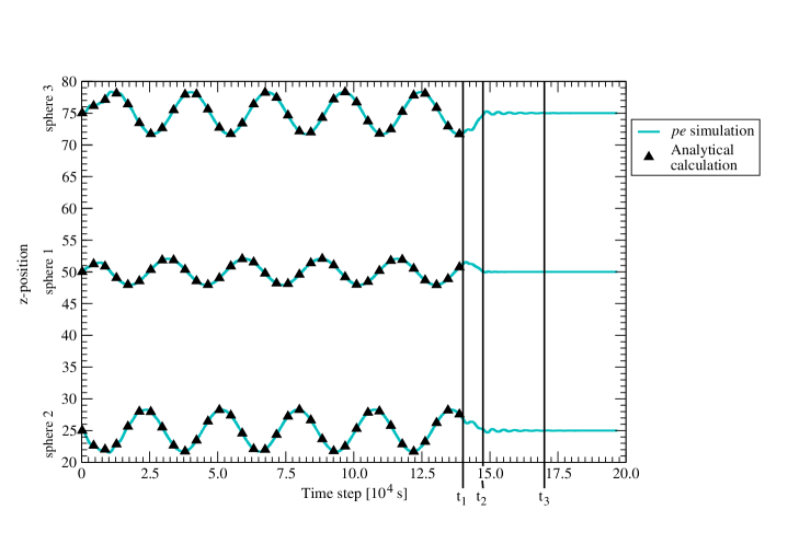
Figure 10: Plot of the z-positions of the three spheres vs. time (weak damping) of one of our simulations. The values of the parameters used are: $m=5.44\times 10^{-13}$ kg, $k=1.72965$ kg/s², $(\vec{l}_{0})_{z}=25$ lattice cells (with discretization $\Delta x=10^{-6}$ m), $\gamma=1.57237\times 10^{-7}$ kg/s, $\omega=296057.86703$ 1/s, $a=1.0\times 10^{-5}$ kg m/s², $\left(\vec{x}_{2}(0)\right)_{z}=25$ lattice cells, $\left(\vec{x}_{1}(0)\right)_{z}=50$ lattice cells, $\left(\vec{x}_{3}(0)\right)_{z}=75$ lattice cells, $\dot{\vec{x}}_{2}(0)=\vec{0}$ m/s, $\dot{\vec{x}}_{1}(0)=\vec{0}$ m/s, $\dot{\vec{x}}_{3}(0)=\vec{0}$ m/s. The simulation is run for 196812 time steps, while the driving force on the left body is switched off at $t_{1}=140580$ time steps, and on the right and hence also on the middle body at $t_{2}=147609$ time steps. The springs obtain their starting configuration at $t_{3}\approx 179000$ time steps.

Figure 10 shows both the simulation and the analytically calculated results for a typical variation of the sphere positions with time in vacuum, in the case of weak damping. The used parameter values are stated in the caption. This particular setup of the damped harmonic oscillators and the driving forces is equal to the setup for the fluid simulation in Section 5. For this number of time steps the lattice Boltzmann algorithm is stable and we also end up in the Stokes regime. As expected, each sphere performs an oscillatory motion in the steady state with its frequency being the same as the driving frequency. Moreover, Figure 10 indicates the force neutrality of our total cycle. After we switch off the driving force on the left body at $t_{1}=140580$ time steps and on the right body and hence also on the middle body at $t_{2}=147609$ time steps (which equal 3/4 of the total time steps), the springs in our swimmer start to revert to their rest lengths, and the swimmer soon obtains its starting configuration at $t_{3}\approx 179000$ time steps, causing the flat ends of the position curves.

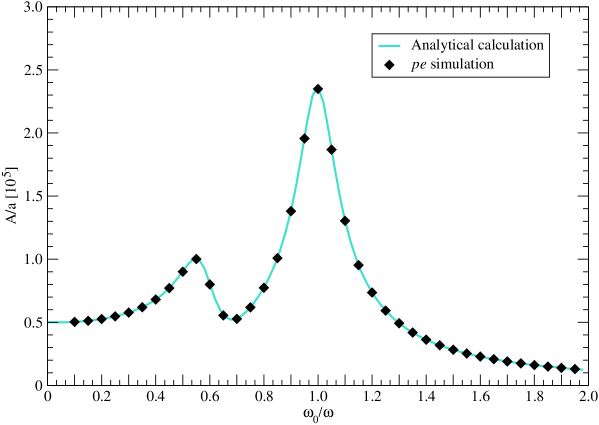
Figure 11: Amplitude of oscillation $A$ scaled by amplitude of the driving forces $a$ (both given on the lattice) on the example of sphere 2 vs. $\omega_{0}/\omega$, with $\omega$ fixed at a value of $296057.86703$ 1/s, for very weak damping ($D=0.07$).

Figure 11 shows the graph of the amplitude of the oscillation $A$ of the sphere 2 (scaled by the amplitude of the driving forces $a$) as a function of the natural spring frequency $\omega_{0}=\sqrt{k/m}$ (scaled by constant $\omega$), with the fixed characteristic damping ratio $D=0.07$ (equation (11)).

For this graph, the mass of each sphere was fixed at $m=5.44\times 10^{-13}$ kg, while the stiffness $k$ of the spring was varied between the values of $4.76813\times 10^{-3}$ kg/s² and $0.181309$ kg/s². Accordingly, the damping $\gamma$ lies within the bounds of $2.27017\times 10^{-9}$ kg/s and $4.414\times 10^{-8}$ kg/s. Both ranges yield a damping ratio of $D=0.07$ in each run. In order to guarantee the achievement of a steady state in all of the simulations, we perform $10^{6}$ time steps.

Both Figure 10 and 11 demonstrate excellent agreement between the simulation results and the analytically obtained results. In Figure 11, the 38 selected simulation scenarios match the analytically obtained curve with the two characteristic maxima at $\omega_{0}\sim\omega$ and $\omega_{0}\sim\omega/\sqrt{3}$ for not less than 10 digits.

5 Simulation of swimmers in a fluid

In the following we perform simulations of swimmers in a highly viscous fluid. Apart from exploring the parameter space in order to achieve simulations in a physically-stable regime, we also show that the shape of a swimmer has a considerable effect on its swimming velocity.

5.1 Parameters of simulations

The setup of the domain for the design parameter study is a cuboidal channel with $(x\times y\times z)=(100\times 100\times 200)$ lattice cells, each of which is a cube with a side length of $10^{-6}$ m. The z-axis corresponds to the axis of movement of the device. The highly viscous fluid has a kinematic viscosity of $\nu=7.36\times 10^{-5}$ m²/s and a density of $\rho=1.36$ kg/m³, these being typical values at room temperature for honey. In order to make the different designs comparable, the mass of all spheres and capsules has been set to $m_{\text{sph}}=m_{\text{cap}}=5.44\times 10^{-13}$ kg. The spheres in the designs (a)-(e), (g)-(j) and (l)-(o) all have the radius $r_{\text{sph}}=4\times 10^{-6}$ m. The capsules used in the designs (b)-(p) all have the radius $r_{\text{cap}}=4\times 10^{-6}$ m and the length $l_{\text{cap}}=8\times 10^{-6}$ m. In order to observe the influence of the distances to the walls of the simulation box, we also consider a three-sphere swimmer (q) with larger radii $r_{\text{sphbig}}=8\times 10^{-6}$ m.

At $t=0$, the swimmer is centered in the channel, with the center of the middle body being at the center of the channel with respect to all three dimensions. As the time-steps increase, the z-positions of the different bodies of the swimmer change, while the x- and the y-positions do not. Also, at $t=0$, the springs are at their rest length of 8 lattice cells ($=8\times 10^{-6}$ m) in the designs (a)-(f) and (l)-(q). In order to make the respective armlengths of the corresponding designs (b)-(f) and (g)-(k) equal, the springs in the designs (g)-(k) have a rest length of 16 lattice cells ($=16\times 10^{-6}$ m) between perpendicular capsules, and those between a sphere and a perpendicular capsule have a rest length of 12 lattice cells ($=12\times 10^{-6}$ m). The other springs in those designs have a rest length of 8 lattice cells ($=8\times 10^{-6}$ m). All springs are characterized by a stiffness of $k=1.72965$ kg/s² and a damping constant of $\gamma=1.57237\times 10^{-7}$ kg/s. This results in a damping ratio of $D=0.07\ll 1$, i.e. our system is in the weak damping regime.

The simulations run for $196812$ time steps, performing five swimming cycles with an oscillation period of $T=28116$ time steps. The sinusoidal driving forces on the left and the middle body are applied at $T=0$, whereas the force on the right body is implemented with a delay of $\varphi=T/4=7029$ time steps. The amplitude of the driving force on the right and the left body is $a=1.0\times 10^{-5}$ kg m/s². The force on the middle body is at each instant the negative of the sum of the forces on the two other bodies, so that the swimmer has no net external driving force at any time step. This means that the amplitude of the driving force on the middle body is $a$ for $t\leq 7029$ and $t\geq 140580$ time steps, and $\sqrt{2}a$ otherwise. All simulations are terminated by switching off the driving at $t_{1}=140580$ time steps for the left body and $t_{2}=147609$ time steps (which equals 3/4 of the total simulation time) for all other bodies and the system is allowed to relax on its own for the remaining time. It should be noted that the same driving forces are applied on the bodies in each simulation, and any differences in their motion are due to their different shapes.

Design		Rest	Total	$Re_{\text{swim}}[10^{-3}]$	$Re^{B_{2}}$	$Re^{B_{1}}$	$Re^{B_{3}}$
		Length	Width
(a)		40	8	6.51	0.066	0.059	0.078
(b)		48	8	6.32	0.128	0.047	0.130
(c)		48	8	5.75	0.053	0.123	0.081
(d)		48	8	6.14	0.074	0.060	0.121
(e)		56	8	5.72	0.143	0.047	0.130
(f)		64	8	5.51	0.119	0.096	0.136
(g)		44	16	5.07	0.064	0.041	0.086
(h)		48	16	4.93	0.047	0.065	0.083
(i)		44	16	4.93	0.077	0.060	0.053
(j)		48	16	3.64	0.074	0.042	0.059
(k)		56	16	3.72	0.056	0.044	0.063
(l)		40	16	4.86	0.062	0.041	0.085
(m)		40	16	4.54	0.045	0.063	0.078
(n)		40	16	4.64	0.078	0.058	0.050
(o)		40	16	3.64	0.074	0.041	0.054
(p)		40	16	3.53	0.051	0.041	0.053
(q)		64	16	2.33	0.080	0.061	0.083

Table 1: Parameters of the different swimmers. $Re^{B_{i}}$ denotes the Reynolds number of the $i$th body in each swimmer, while $Re_{\text{swim}}$ indicates the Reynolds number of the whole swimmer.

5.2 Stability

We show that our choice of parameters results in our swimmers being in the regime of low Reynolds numbers [32]. The latter is given by

$$Re=\frac{u\,l}{\nu}\ll 1,$$ (24)

with the kinematic viscosity of the fluid $\nu$, the characteristic velocity $u$ and the characteristic length-scale $l$.

In order to simulate our swimmer in a stable regime, we define two different Reynolds numbers. The first is the Reynolds number of the whole swimming device (Table 1, fourth column), defined as

$$Re_{\text{swim}}=\frac{u_{\text{swim}}\,l_{\text{swim}}}{\nu}\ll 1$$ (25)

with respect to the characteristic velocity of the swimmer $u_{\text{swim}}$. The latter is calculated from the movement $\Delta$ of the central body in the swimmer during one swimming cycle (here chosen to be the last full cycle), divided by the time-period $T$, i.e. $u_{\text{swim}}=\Delta/T$. The characteristic length-scale $l_{\text{swim}}$ of the different swimming devices is the rest length in the direction of motion for all the different swimmer designs (Table 1, second column).

Additionally, we verify the Reynolds number not only for the whole swimmer but also for each of the bodies (Table 1, third, fourth and fifth column), which may move with considerably higher velocities than the swimming device. Here, the Reynolds number of the body $B_{i}$ is

$$Re^{B_{i}}=\frac{u^{B_{i}}\,l^{B_{i}}}{\nu}\ll 1,$$ (26)

and $u^{B_{i}}$ is the maximum velocity of the body $B_{i}$ and $l^{B_{i}}$ is its length in the direction of motion. As Table 1 confirms, all the Reynolds numbers satisfy the $Re\ll 1$ condition.

5.3 Swimming velocities

In the following, we investigate the performance of each swimmer as a function of its design geometry, as also detailed in Pickl et al. [29]. Specifically, we study the dependence of the amplitudes of the oscillations of the bodies in each swimmer on their shapes, and relate this to the overall swimming velocity.

5.3.1 The three-sphere swimmers

First we look at the two swimmers which consist solely of spheres. Table 2 shows the velocity of each swimmer obtained from the simulations ($u_{\text{swim}}$). We find that the swimmer consisting of smaller spheres moves significantly faster than the one with larger spheres. Figure 12 shows the plot of the simulation trajectories of each body in the two swimmers.

Design		$u_{\text{swim}}[10^{-6}]$	$u_{\text{GA}}[10^{-6}]$	Error	Efficiency $[10^{-4}]$
(q)		2.02	2.45	$<18\%$	0.88
(a)		9.05	8.98	$<1\%$	10.44

Table 2: Comparison of swimming velocities from the simulations ($u_{\text{swim}}$) and from the prediction of Golestanian and Ajdari ($u_{\text{GA}}$), in the case of spheres. All the quantities are given in terms of their values on the lattice.

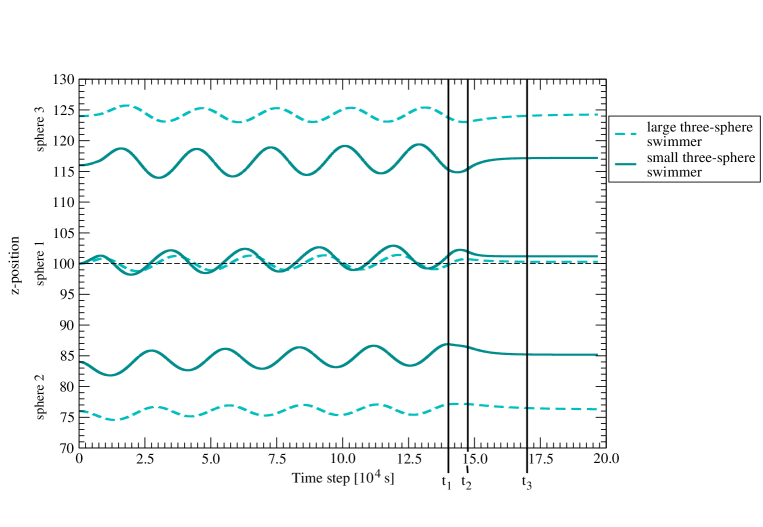
Figure 12: Trajectories of each sphere in the two three-sphere swimmers. The dashed curves and the solid curves show the trajectories of the spheres in the large and the small swimmer, respectively. The simulation is run for 196812 time steps, while the driving force on the left body is switched off at $t_{1}=140580$ time steps, and on the right and hence also on the middle body at $t_{2}=147609$ time steps. The springs obtain their starting configuration at $t_{3}\approx 179000$ time steps.

In previous work, this design has been analytically modeled by Golestanian and Ajdari [12], who predict the velocity of a swimmer (here called $u_{\text{GA}}$, Table 2, third column) if the amplitude of oscillation of its two arms is known. Here, an arm is defined as the distance between the centers of two bodies connected by a spring. In their model, Golestanian and Ajdari assume that the deformation of each arm is given by

$$l_{i}(t)=\bar{l}_{i}+d_{i}\cos(\omega t+\varphi_{i}),\,\,\,\,\,i=1,2$$ (27)

Here $\bar{l}_{i}$ is the average length and $l_{i}(t)$ the instantaneous length of arm $i$, and $d_{i}$, $\omega$ and $\varphi_{i}$ are the amplitude, the frequency and the phase shift of the oscillation of arm $i$. Under these conditions, the formula for the average velocity of a three-sphere swimmer is

$$u_{\text{GA}}=K\,d_{1}\,d_{2}\,\omega\,\sin(\varphi_{1}-\varphi_{2})$$ (28)

where $K$ is a geometrical factor given by

$$K=\frac{3r_{1}r_{2}r_{3}}{2(r_{1}+r_{2}+r_{3})^{2}}\left[\frac{1}{\bar{l}_{1}^{2}}+\frac{1}{\bar{l}_{2}^{2}}-\frac{1}{(\bar{l}_{1}+\bar{l}_{2})^{2}}\right].$$ (29)

Here, $r_{1},r_{2}$ and $r_{3}$ are the radii of the three spheres. It is also assumed that $r_{i}\ll\bar{l}_{j}$ and $d_{i}\ll\bar{l}_{j}$, for all $i$ and $j$.

Since this model assumes a velocity protocol in contrast to our force protocol (i.e., we start off with known forces which are applied on the bodies whereas the model of Golestanian and Ajdari assumes known deformations of the arms, regardless of the forces that cause them), we first extract $\{d_{i}\}$ and $\{\varphi_{i}\}$ from the simulation trajectories (Table 3), and use them with the known values of $\{\bar{l}_{i}\}$, $\{r_{i}\}$ and $\omega$ to find $u_{\text{GA}}$ from equation (28). To extract $\{d_{i}\}$ and $\{\varphi_{i}\}$, we fit the armlength trajectories for the last complete period of motion (from $t=4T$ to $t=5T$) with equation (27).

Design		$K$	$d_{1}$	$d_{2}$	$\sin(\varphi_{1}-\varphi_{2})$
(q)		0.0040	1.59	2.07	0.83
(a)		0.0045	2.53	3.80	0.94

Table 3: Parameters for the three-sphere swimmers. $\omega$ equals 0.00022. All the quantities are given in terms of their values on the lattice.

We define the error in $u_{\text{swim}}$, when compared with the theoretically-expected $u_{\text{GA}}$ value, as

$$\text{Error}=\left|\dfrac{u_{\text{GA}}-u_{\text{swim}}}{u_{\text{GA}}}\right|\times 100.$$ (30)

For the swimmer with large spheres, this error comes out to be 18%. This is possibly explained by the effect of the boundaries of the simulation box on the spheres of the larger swimmer. The theoretical result assumes infinite fluid, whereas the simulations are conducted in a finite box of the dimensions stated above. Another possible reason for the disagreement in the two velocities for the large-spheres swimmer is that the condition $r_{i}\ll\bar{l}_{j}$ is not satisfied very well. For the swimmer with small spheres, the effect of the finiteness of the swimming domain is smaller, and the $r_{i}\ll\bar{l}_{j}$ condition is also satisfied to a greater extent. Consequently, we find that in this case there is excellent agreement between $u_{\text{GA}}$ and $u_{\text{swim}}$, to an error of less than 1% (Table 2). We also observe that for the swimmer with small spheres, the amplitude of oscillation of each arm is larger than that of the corresponding arm for the larger swimmer (Table 3, third column)), and that for each swimmer, the amplitude of oscillation of the leading arm ($d_{2}$) is greater than that of the trailing arm ($d_{1}$).

Table 2 also shows the swimming efficiency of the two swimmers, as defined by Lighthill [23],

$$\text{Efficiency}=\frac{6\,\pi\,\eta\,r_{\text{eff}}\,u_{\text{swim}}^{2}}{\frac{1}{T}\int_{4T}^{5T}\sum_{i}\vec{F}_{\text{dri}}^{B_{i}}(t)\cdot\vec{u}^{B_{i}}(t)\,dt}.$$ (31)

Here $r_{\text{eff}}$ is an effective hydrodynamic radius of the swimmer, and is approximated by the sum of the radii of the three spheres [1]. $\vec{u}^{B_{i}}(t)$ is found from the simulation curves, using the last full swimming cycle (i.e., from $t=4T$ to $t=5T$). The integration is also done over this period, in order to work with the steady-state values. Table 2 shows that the efficiency of the swimmer with small spheres is greater, as expected due to its significantly greater swimming velocity.

5.3.2 Swimmers with capsules

The rest of the swimmers contain capsules, and can be separated into three distinct families. The first family consists of the swimmers labeled (b)-(f) in Table 1. These contain capsules which are parallel to the swimming direction (henceforth referred to as parallel capsules), and have springs of a rest length of 8 lattice cells. The second family consists of the swimmers labeled (g)-(k) in Table 1. These contain capsules which are perpendicular to the swimming direction (henceforth referred to as perpendicular capsules), and have springs of a rest length of 8, 12 or 16 lattice cells. The third family consists of the swimmers labeled (l)-(p) in Table 1. These also contain perpendicular capsules, and their springs all have a rest length of 8, making these swimmers shorter than the swimmers in the second family.

Tables 4, 5 and 6 (second column) show the measured $u_{\text{swim}}$ for the swimmers with parallel capsules, with perpendicular capsules and longer springs, and with perpendicular capsules and shorter springs, respectively. In all the three tables, the swimmers are arranged in the increasing order of $u_{\text{swim}}$, from top-to-bottom. It can be observed that corresponding designs in each family occupy the same position in their respective tables. Here, two designs are said to be corresponding if one needs to replace the same spheres in a three-sphere swimmer to get both the designs, albeit by different kinds of capsules (and, possibly, with springs of different lengths). One also observes that the speed of swimming decreases with an increase in the number of capsules. This can be attributed to the fact that the small spheres have greater amplitudes of oscillation than the capsules, which means that the lengths of arms which contain spheres have greater amplitudes of oscillation than those that do not. A greater amplitude of oscillation of the arms results in a higher swimming velocity.

Design		$u_{\text{swim}}[10^{-6}]$	$u_{\text{GA}}[10^{-6}]$	Error	Efficiency $[10^{-4}]$
(f)		4.78	4.50	$<7\%$	3.69
(e)		5.68	5.48	$<4\%$	5.31
(c)		6.66	6.31	$<6\%$	5.86
(d)		7.11	7.16	$<1\%$	7.37
(b)		7.32	7.21	$<2\%$	7.77

Table 4: Comparison of swimming velocities from the simulations ($u_{\text{swim}}$) and from the prediction of Golestanian and Ajdari ($u_{\text{GA}}$), in the case of the swimmers with parallel capsules. All the quantities are given in terms of their values on the lattice.

Design		$u_{\text{swim}}[10^{-6}]$	$u_{\text{GA}}[10^{-6}]$	Error	Efficiency $[10^{-4}]$
(k)		3.69	3.95	$<7\%$	2.12
(j)		4.21	4.66	$<10\%$	3.08
(h)		5.71	6.50	$<13\%$	4.24
(i)		6.23	6.75	$<8\%$	5.74
(g)		6.40	6.82	$<7\%$	5.97

Table 5: Comparison of swimming velocities from the simulations ($u_{\text{swim}}$) and from the prediction of Golestanian and Ajdari ($u_{\text{GA}}$), in the case of the second family of the swimmers with capsules. All the quantities are given in terms of their values on the lattice.

Design		$u_{\text{swim}}[10^{-6}]$	$u_{\text{GA}}[10^{-6}]$	Error	Efficiency $[10^{-4}]$
(p)		4.90	6.70	$<27\%$	3.63
(o)		5.05	6.63	$<24\%$	4.08
(m)		6.30	8.96	$<30\%$	4.76
(n)		6.44	7.74	$<17\%$	5.93
(l)		6.75	7.66	$<12\%$	6.47

Table 6: Comparison of swimming velocities from the simulations ($u_{\text{swim}}$) and from the prediction of Golestanian and Ajdari ($u_{\text{GA}}$), in the case of the third family of the swimmers with capsules. All the quantities are given in terms of their values on the lattice.

The simulation trajectories of all swimmers with capsules show that irrespective of the number of capsules in the swimmer, each body exhibits a smooth sinusoidal movement in the steady state, and one may attempt to use the formula of Golestanian and Ajdari (equation (28)) for the analysis of the swimming motion. While this formula was developed assuming the bodies to be spherical, one may hypothesize that small deviations from the spherical shapes of the bodies will mostly affect the geometrical pre-factor $K$ in equation (28) and not the general expression. We test this hypothesis by extracting the amplitudes of the body oscillations and their phase shifts by fitting the trajectories with equation (27). The geometric factor is obtained by approximating each capsule by a sphere of diameter 12, as that is the arithmetic mean of the dimensions of each capsule in the direction of movement and in a direction perpendicular to it. The mean armlengths are the same as in the original swimmers. For ease of reference, the values of all of these parameters are given in the appendix (tables 7, 8 and 9). These tables show that as in the case of the three-sphere swimmers, the amplitude of oscillation of the leading arm ($d_{2}$ in the tables) is larger than that of the trailing arm ($d_{1}$ in the tables), for each swimmer.

The second and the third columns of the Tables 4, 5 and 6 show the estimated $u_{\text{GA}}$ and the error in the measured $u_{\text{swim}}$ relative to $u_{\text{GA}}$ for each of the three families. It is interesting to note that the $u_{\text{GA}}$ approximation is still in good agreement with the results of the simulations. Especially in the first two families the error is about 10% or less. For the third family, i.e. for the swimmers with perpendicular capsules and shorter springs, the errors increase, to between 10% and 30%, probably because our approximation causes the spring lengths to become smaller than or equal to the sphere radii. Therefore the conditions necessary for the validity of Golestanian and Ajdari’s formula are compromised. This is similar to the case of the three-sphere swimmer with large spheres, where the calculated and the observed velocities of the swimmer also disagreed due to the $r_{i}\ll\bar{l}_{j}$ condition not being satisfied well.

The tables also show the efficiencies, as defined in equation (31), of the swimmers in each family. Here, the hydrodynamic radius $A$ has been calculated by assuming, as before, that each capsule is replaced by a sphere of diameter 12. The results show that in each family, the order of the efficiencies accords with the order of $u_{\text{swim}}$. This is as expected, since the driving forces for each swimmer in all our simulations are exactly the same, and so a more efficient swimmer would be expected to move faster than a less efficient one.

While this comparison has provided some useful insights, in order to fully understand our simulation results, the theory of Golestanian and Ajdari should be expanded to account for capsules, a task that we hope to undertake in the future.

6 Conclusions and Future Work

In this work we have demonstrated the successful integration of self-propelled micro-devices into the coupled $\mathpzc{pe}$-waLBerla framework. Furthermore, we have shown the validity of this approach by comparing the results of simulations to analytical models. We have taken advantage of the flexibility of our framework to simulate symmetric and asymmetric swimmers combining capsule and sphere geometries, which has not been possible so far.

The establishment of this framework is especially important for the study of systems that are inaccessible via experimental and analytical methods. In the future, we aim to harness its capabilities to address issues such as the problem of the three-body swimmer in regimes beyond those dictated by the approximations of Felderhof [11] and Golestanian and Ajdari [12]. Another interesting application would be to study the behavior of the swimmer in a narrow channel and explore the role of the boundary conditions at the wall.

It would also be interesting to investigate the hydrodynamic interactions amongst many swimmers swimming together [13, 19]. In Figure 13 we show the flow fields averaged over five cycles for the case of a single swimmer and also for three swimmers swimming together. The simulation of the three swimmers took 60.28 hours of total CPU-time on a single Intel Core i5-680 3.60GHz. To exclude the effects of the walls of the channel, one needs to set up even larger flow fields around the swimmers in this case than in the case of a single swimmer. Moreover, our work indicates that a steady state is reached after a significantly longer time in the case of many swimmers swimming together compared to the case of a single swimmer.

These factors suggest that in the current setting, the accurate simulation of many swimmers would take very long. To reduce this simulation time significantly, the large domains of simulation should be processed in a more efficient way by parallelizing the framework. Both waLBerla and $\mathpzc{pe}$ already feature massively parallel simulation algorithms for large scale particulate flow scenarios [15], but the parallelization of the force generators (i.e. springs) and velocity constraints is yet to be implemented. Once this is achieved, massive simulations with a large number of swimmers will be accessible, allowing us, finally, to address the problem of swarming.

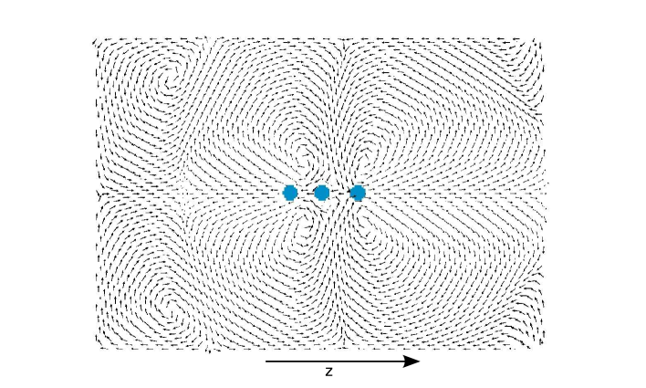
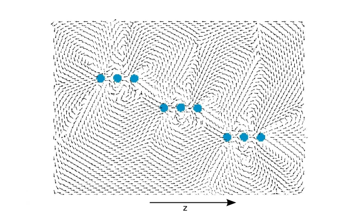
Figure 13: Flow field of one and three three-sphere swimming devices, averaged over five swimming cycles. We used the same parameters for the simulation setup as in Section 5.1, except for the channel, which now is $(x\times y\times z)=(164\times 164\times 240)$ lattice cells.

Appendix A Values of different parameters of the swimmers with capsules

Here we present the values of the different parameters of the swimmers with capsules, found from the simulation curves and used in equation (28).

Design		$K$	$d_{1}$	$d_{2}$	$\sin(\varphi_{1}-\varphi_{2})$
(f)		0.0030	2.24	3.39	0.89
(e)		0.0037	2.21	3.63	0.84
(c)		0.0032	2.59	3.59	0.96
(d)		0.0041	2.47	3.65	0.87
(b)		0.0041	2.26	3.79	0.92

Table 7: The different parameters for the swimmers with parallel capsules. $\omega$ equals 0.00022. All the quantities are given in terms of their values on the lattice.

Design		$K$	$d_{1}$	$d_{2}$	$\sin(\varphi_{1}-\varphi_{2})$
(k)		0.0030	2.14	3.26	0.85
(j)		0.0037	2.11	3.62	0.75
(h)		0.0032	2.66	3.57	0.97
(i)		0.0041	2.43	3.65	0.84
(g)		0.0041	2.17	3.80	0.91

Table 8: The different parameters for the swimmers with perpendicular capsules and long springs. $\omega$ equals 0.00022. All the quantities are given in terms of their values on the lattice.

Design		$K$	$d_{1}$	$d_{2}$	$\sin(\varphi_{1}-\varphi_{2})$
(p)		0.0068	1.92	2.59	0.90
(o)		0.0058	2.07	3.33	0.76
(m)		0.0050	2.56	3.24	0.98
(n)		0.0050	2.54	3.39	0.81
(l)		0.0050	2.00	3.75	0.92

Table 9: The different parameters for the swimmers with perpendicular capsules and short springs. $\omega$ equals 0.00022. All the quantities are given in terms of their values on the lattice.

References

- Alouges et al. [2009] F. Alouges, A. DeSimone, A. Lefebvre, Optimal strokes for axisymmetric microswimmers, The European Physical Journal E: Soft Matter and Biological Physics 28 (2009) 279–284.
- Anitescu and Potra [1997] M. Anitescu, F.A. Potra, Formulating dynamic multi-rigid-body contact problems with friction as solvable linear complementarity problems, Nonlinear Dynamics 14 (1997) 231–247.
- Bhatnagar et al. [1954] P.L. Bhatnagar, E.P. Gross, M. Krook, A model for collision processes in gases. I. Small amplitude processes in charged and neutral one-component systems, Physical Review 94 (1954) 511–525.
- Binder et al. [2006] C. Binder, C. Feichtinger, H. Schmid, N. Thürey, W. Peukert, U. Rüde, Simulation of the hydrodynamic drag of aggregated particles, Journal of Colloid and Interface Science 301 (2006) 155–167.
- Chang et al. [2007] S.T. Chang, V.N. Paunov, D.N. Petsev, O.D. Velev, Remotely powered self-propelling particles and micropumps based on miniature diodes, Nature Materials 6 (2007) 235–240.
- Chen and Doolen [1998] S. Chen, G.D. Doolen, Lattice Boltzmann method for fluid flows, Annual Review of Fluid Mechanics 30 (1998) 329–364.
- Cundall and Strack [1979] P.A. Cundall, O.D.L. Strack, A discrete numerical model for granular assemblies, Geotechnique 29 (1979) 47–65.
- Dreyfus et al. [2005] R. Dreyfus, J. Baudry, M. Roper, M. Fermigier, H.A. Stone, J. Bibette, Microscopic artificial swimmers, Nature 437 (2005) 862–865.
- Earl et al. [2007] D.J. Earl, C.M. Pooley, J.F. Ryder, I. Bredberg, J.M. Yeomans, Modeling microscopic swimmers at low Reynolds number, Journal of Chemical Physics 126 (2007) 064703.
- Feichtinger et al. [2011] C. Feichtinger, S. Donath, H. Köstler, J. Götz, U. Rüde, WaLBerla: HPC software design for computational engineering simulations, Journal of Computational Science In Press, Corrected Proof (2011).
- Felderhof [2006] B.U. Felderhof, The swimming of animalcules, Physics of Fluids 18 (2006) 063101.
- Golestanian and Ajdari [2008] R. Golestanian, A. Ajdari, Analytic results for the three-sphere swimmer at low Reynolds number, Physical Review E 77 (2008) 036308.
- Golestanian et al. [2011] R. Golestanian, J. Yeomans, N. Uchida, Hydrodynamic synchronization at low Reynolds number, Soft Matter 7 (2011) 3074–3082.
- Götz et al. [2010a] J. Götz, K. Iglberger, C. Feichtinger, S. Donath, U. Rüde, Coupling multibody dynamics and computational fluid dynamics on 8192 processor cores, Parallel Computing 36 (2010a) 142–141.
- Götz et al. [2010b] J. Götz, K. Iglberger, M. Stürmer, U. Rüde, Direct numerical simulation of particulate flows on 294912 processor cores, in: 2010 ACM/IEEE International Conference for High Performance Computing, Networking, Storage and Analysis, IEEE, pp. 1–11.
- Iglberger [2010] K. Iglberger, Software Design of a Massively Parallel Rigid Body Framework, Ph.D. thesis, 2010.
- Iglberger and Rüde [2010] K. Iglberger, U. Rüde, Massively parallel granular flow simulations with non-spherical particles, Computer Science - Research and Development 25 (2010) 105–113.
- Iglberger et al. [2008] K. Iglberger, N. Thürey, U. Rüde, Simulation of moving particles in 3D with the lattice Boltzmann method, Computers & Mathematics with Applications 55 (2008) 1461–1468.
- Kanevsky et al. [2010] A. Kanevsky, M.J. Shelley, A.K. Tornberg, Modeling simple locomotors in Stokes flow, Journal of Computational Physics 229 (2010) 958–977.
- Körner et al. [2005] C. Körner, T. Pohl, U. Rüde, N. Thürey, T. Zeiser, Parallel lattice Boltzmann methods for CFD applications, in: A. Bruaset, A. Tveito (Eds.), Numerical Solution of Partial Differential Equations on Parallel Computers, volume 51 of Lecture Notes for Computational Science and Engineering, Springer Verlag, 2005, pp. 439–465.
- Kosa et al. [2007] G. Kosa, M. Shoham, M. Zaaroor, Propulsion method for swimming microrobots, Robotics, IEEE Transactions on 23 (2007) 137 –150.
- Lauga and Powers [2009] E. Lauga, T.R. Powers, The hydrodynamics of swimming microorganisms, Reports on Progress in Physics 72 (2009) 096601.
- Lighthill [1952] M.J. Lighthill, On the squirming motion of nearly spherical deformable bodies through liquids at very small Reynolds numbers, Communications on Pure and Applied Mathematics 5 (1952) 109–118.
- Lorenz et al. [2009] E. Lorenz, A. Caiazzo, A.G. Hoekstra, Corrected momentum exchange method for lattice Boltzmann simulations of suspension flow, Physical Review E 79 (2009) 036705.
- Mei et al. [2006] R. Mei, L.S. Luo, P. Lallemand, D. d’Humières, Consistent initial conditions for lattice Boltzmann simulations, Computers & Fluids 35 (2006) 855 – 862. Proceedings of the First International Conference for Mesoscopic Methods in Engineering and Science.
- Mei et al. [2002] R. Mei, W. Shyy, D. Yu, L.S. Luo, Lattice Boltzmann method for 3-D flows with curved boundary, Journal of Computational Physics 161 (2002) 680–699.
- Najafi and Golestanian [2004] A. Najafi, R. Golestanian, Simple swimmer at low Reynolds number: Three linked spheres, Physical Review E 69 (2004) 062901.
- Pickl [2009] K. Pickl, Rigid Body Dynamics: Links and Joints, Master’s thesis, Computer Science Department 10 (System Simulation), University of Erlangen-Nürnberg, 2009.
- Pickl et al. [2011] K. Pickl, J. Pande, J. Götz, K. Iglberger, U. Rüde, K. Mecke, A. Smith, The effect of shape on the efficiency of self-propelled swimmers, submitted to Physical Review Letters (2011).
- Pohl et al. [2003] T. Pohl, M. Kowarschik, J. Wilke, K. Iglberger, U. Rüde, Optimization and profiling of the cache performance of parallel lattice Boltzmann codes, Parallel Processing Letters 13 (2003) 549–560.
- Pooley and Yeomans [2008] C.M. Pooley, J.M. Yeomans, Lattice Boltzmann simulation techniques for simulating microscopic swimmers, Computer Physics Communications 179 (2008) 159 – 164.
- Purcell [1977] E.M. Purcell, Life at low Reynolds number, American Journal of Physics 45 (1977) 3–11.
- Putz and Yeomans [2009] V. Putz, J.M. Yeomans, Hydrodynamic synchronisation of model microswimmers, Journal of Statistical Physics 137 (2009) 1001–1013.
- Qian et al. [1992] Y.H. Qian, D. d’Humières, P. Lallemand, Lattice BGK models for Navier-Stokes equation, Europhysics Letters (EPL) 17 (1992) 479–484.
- Succi [2001] S. Succi, The Lattice Boltzmann Equation - For Fluid Dynamics and Beyond, Clarendon Press, 2001.
- Taylor [1951] G. Taylor, Analysis of the swimming of microscopic organisms, Proceedings of the Royal Society of London. Series A. Mathematical and Physical Sciences 209 (1951) 447–461.
- Wellein et al. [2005] G. Wellein, T. Zeiser, S. Donath, G. Hager, On the single processor performance of simple lattice Boltzmann kernels, Computer & Fluids 35 (2005) 910–919.
- Yang et al. [2010] Y.Z. Yang, V. Marceau, G. Gompper, Swarm behavior of self-propelled rods and swimming flagella, Physical Review E 82 (2010) 031904.
- Yu et al. [2003] D. Yu, R. Mei, L.S. Luo, W. Shyy, Viscous flow computations with the method of lattice Boltzmann equation, Progress in Aerospace Sciences 39 (2003) 329–367.