The Unequal Twins - Probability Distributions Aren’t Everything

Abstract

It is the common lore to assume that knowing the equation for the probability distribution function (PDF) of a stochastic model as a function of time tells the whole picture defining all other characteristics of the model. We show that this is not the case by comparing two exactly solvable models of anomalous diffusion due to geometric constraints: The comb model and the random walk on a random walk (RWRW). We show that though the two models have exactly the same PDFs, they differ in other respects, like their first passage time (FPT) distributions, their autocorrelation functions and their aging properties.

One often thinks that perfect knowledge of the PDF as a function of time (achieved by better experimental techniques or by data mining) completely determines the underlying stochastic model. In what follows we illustrate that this is not the case by revisiting two exactly solvable models often invoked when explaining anomalous diffusion in labyrinthine structures of percolation type: the comb model introduced in Weiss and Havlin (1986) (which mimics trapping in the dangling ends) and the RWRW introduced in Kehr and Kutner (1982) (which mimics the tortuosity of the chemical path). Both are visualized in Fig. 1. The RWRW model was introduced as a simplified (quenched) version of the single-file diffusion. In polymer physics, the RWRW corresponds to one of the regimes of reptation Doi and Edwards (1988), namely, to the motion of the chain as a whole along its primitive path. These facts make evident its relation to other models of diffusion under time-dependent constraints, which are often described using a fractional Brownian motion approach. Although both models are known for around quarter of a century and were quite carefully investigated, the two were never confronted. Doing so is however quite instructive. Thus in the long time limit both models, the comb (of the CTRW class Weiss and Havlin (1986)) and the RWRW (in a class of itself, but a close relative of the single file diffusion) show exactly the same PDF which can be described by the corresponding fractional diffusion equation Metzler and Klafter (2000). However, the models differ in any other respect: the comb model exhibits aging while the RWRW does not, the distribution of FPTs to a given site are different and also the auto-correlation functions differ.

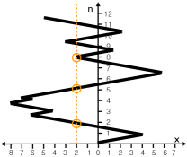
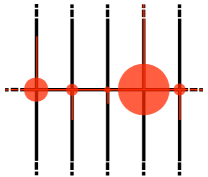
Figure 1: (color online) Left: RWRW model. The trajectory of a random walk (acting as a track on which a RWer may move) is displayed in black. Circles mark the position $x=-2$ at different ’chemical distances’ along the track. Right: A RW on a symmetric comb structure. The RW trajectory is marked in a lighter shade (red). The projection of the trajectory on the $x$-axis, or backbone, leads to waiting times caused by the RW’s sojourn in a tooth (depicted by circles of sizes representing the appropriate waiting time), thus a CTRW.

Note that both the comb and RWRW models stem from Markovian random walk (RW) models on the corresponding geometries, i.e., the probabilities of steps from a site $(i,j)$ on the underlying track depend only on the position $(i,j)$. In both cases the RWs have independent but not identically distributed increments. We are interested in the projection of the RW onto the $x$-axis. The fact that the same value of $x$ may correspond to different values of $y$ in the comb model, or to different positions along the contour length $n$ in the RWRW model (see Fig. 1), and that the further motion depends explicitly on this $y$ or $n$, introduces the memory on the previous positions. Introducing the memory is the cost we pay for neglecting the irrelevant coordinate ($y$ or $n$), the dependence on which however does not disappear. The kind of non-Markovian behavior of the reduced models is strongly different: The diffusion on the comb falls into a semi-Markovian CTRW class, the one on the RW track is an anti-persistent RW, a close relative (but not a member of the class) of fractional Brownian motions.

In the CTRW as represented by the comb model the probability density of being at position $x$ after $n$ time steps is given by the subordination expression

$$p(x,t)=\sum_{n=0}^{\infty}p(x,n)\chi(n,t)\simeq\int_{0}^{\infty}{p(x,n)\chi(n,t)\mathrm{d}n}$$ (1)

where $p(x,n)$ gives the probability of reaching $x$ after $n$ steps and $\chi(n,t)$ is the probability to make $n$ steps within time $t$. Here $t$ is measured in the units of time steps $\tau=1$. Note that for $t\gg\tau$ the typical number of steps $n$ is large and can be considered as a continuous variable, turning the sum in Eq. (1) into an integral over $n$. The waiting time distribution along the comb backbone is given by the return time probability of a RW on a tooth to the backbone, which is approximately $\psi(t)\simeq(2\pi)^{-1/2}t^{-3/2}$ Chandrasekhar (1943). In the Laplace domain, $\chi(n,t)$ and $\psi(t)$ are related via Klafter and Sokolov (2011):

$$\chi(n,s)=s^{-1}[1-\psi(s)]\psi^{n}(s),$$ (2)

where $f(s)$ denotes the Laplace transform of a function $f(t)$. Substituting $\psi(s)\simeq 1-\sqrt{2}s^{1/2}$ into Eq. (2) and performing the inverse Laplace transform results in:

$$\chi(n,t)\simeq\frac{\sqrt{2}}{\sqrt{\pi t}}\exp\left(-\frac{n^{2}}{2t}\right),$$ (3)

a Gaussian distribution restricted to the non-negative half-line. Substituting Eq. (3) and $p(x,n)$ (which tends to a Gaussian for large $n$ for a regular RW on the backbone) into the continuous limit of Eq. (1), we get:

$$p(x,t)=\int_{0}^{\infty}\frac{1}{\sqrt{2\pi n}}\exp\left(-\frac{x^{2}}{2n}\right)\frac{\sqrt{2}}{\sqrt{\pi n}}\exp\left(-\frac{n^{2}}{2t}\right)\mathrm{d}n.$$ (4)

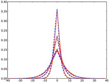
Figure 2: (color online) PDFs of RWRW (smooth red line) vs. RW on a comb (dashed blue line) for a different number of time steps: (a) t=100, (b) t=1000, (c) t=5000, (d) t=6500. It can be clearly seen that the PDFs of the two models coincide.

Let us now calculate the PDF of the particles’ displacement in the RWRW model, pertinent to many realizations of walks and starting points. Let us consider a RW on a RW starting at $x=0$ and consider its position after $t\gg 1$ time steps in a continuous approximation when the displacement $n$ of the RWer along the trajectory of the RW is well-approximated by a Gaussian:

$$\kappa(n,t)\simeq\frac{1}{\sqrt{2\pi t}}\exp\left(-\frac{n^{2}}{2t}\right).$$ (5)

The projection on $x$ of this displacement along the trajectory is again given by a Gaussian depending on the displacement $|n|$:

$$p(x,n)\simeq\frac{1}{\sqrt{2\pi|n|}}\exp\left(-\frac{x^{2}}{2|n|}\right).$$ (6)

The displacement in $x$ as a function of $t$ is expressed by:

$$p(x,t)=\int_{-\infty}^{\infty}p(x,n)\kappa(n,t)\mathrm{d}n.$$ (7)

Substituting Eqs. (5) and (6) into Eq. (7) results in exactly the same expression as Eq. (4). This is numerically verified in Fig. 2. The models are essentially twins!

Let us however stress a fundamental difference between the two models. Eq. (4) implies that the time $t$ is counted from the beginning of the walk starting at $(0,0)$. In the course of time the walker typically enters deeper into the dangling ends. If the observation starts at a later instant $t>0$, the walker will typically need time to return to the $x$-axis to take a step in a relevant direction. Therefore the waiting time PDF for the first step after $t>0$ is different from $\psi(t)$ Klafter and Sokolov (2011), leading to a different $\chi(n,t)$: the diffusion on the comb shows aging typical of CTRW Sokolov et al. (2001a, b). On the contrary, the RWRW model does not age: the same distribution $\kappa(n,t)$ holds, whenever one starts. This property can be inferred from Fig. 3 showing MSDs for both models for observations starting at different times from the beginning of the RW.

Note that the movements in the $x$ and $y$ directions on the comb are correlated: the more steps in the $x$ direction are made, the less time remains for steps in the $y$ direction. The total MSD $\langle r^{2}\rangle=\langle x^{2}\rangle+\langle y^{2}\rangle$ is found to be diffusive, $\langle r^{2}(t)\rangle\sim n$, Sup , which is numerically verified (inset in Fig. 3). It is interesting to note that though the $x$-projection of this RW follows a non-ergodic subdiffusive process, the 2d picture corresponds to ergodic normal diffusion. This emphasizes the importance of vigilance on experimentalists’ side when assuming that a projection onto a lower dimension gives a representative description of the process.

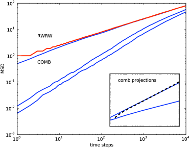
Figure 3: (color online) MSDs in a comb and in a RWRW for different time lags after the beginning of the RW ($\tau=0,1000,3000$). The MSDs for different time lags for the RWRW overlap (upper, red curve). The lower (blue) curves represent the MSDs of the comb model. The larger the time lag the longer it takes the MSD to reach its asymptotic behavior. The inset shows the MSD of the the 2d comb model averaged over time (black dashed line) and over an ensemble (overlapping solid blue), showing the ergodicity of the two-dimensional motion. The behavior of $\langle x^{2}\rangle$ (lower solid blue) is shown for comparison.

Let us now turn to the properties of the process other than the PDF and calculate the FPT distributions for the two models, starting with the comb. As in a general CTRW, the FPT for a comb is given by the subordination formula

$$f(t)=\sum_{n=0}^{\infty}f(n)\psi_{n}(t)$$ (8)

where $f(n)$ is the FPT probability at the $n$-th step in a regular RW and $\psi_{n}(t)$ is the probability density to make the $n$-th step at time instant $t$ (note that the first passage only takes place exactly when the step is taken, so that $\psi_{n}(t)\neq\chi(n,t)$). The FPT of a regular RW is asymptotically given by the Smirnov distribution:

$$f(n)\simeq\frac{|x|}{\sqrt{2\pi}n^{3/2}}\exp\left(-\frac{x^{2}}{2n}\right).$$ (9)

In the continuum limit one may approximate the sum by an integral over $n$. Since in the Laplace domain $\psi_{n}(s)=\psi^{n}(s)$ for $s\to 0$ we have $\psi_{n}(t)\simeq\exp(n(1-\psi(s))$, resulting in $f(s)\sim\int_{0}^{\infty}f(n)e^{-n\sqrt{2s}}dn=e^{-2|x||s|^{1/4}}$, which is the characteristic function of a one-sided Lévy law of index $1/4$. Its behavior for $t\to\infty$ is

$$f(t)\simeq\frac{-2|x|}{\Gamma(-1/4)}t^{-5/4}.$$ (10)

We stress that the same result follows from the solution of the fractional diffusion equation with an absorbing boundary Klafter and Sokolov (2011).

Let us now calculate the FPT distribution for the RWRW model Sup . We fix the starting point $x=0$ and the final point $x_{1}$. The RW track on which the RW then takes place has two strands connecting $x_{0}$ to the two points corresponding to $x_{1}$ (existing due to a recurrence of RWs in 1d). The distances $l_{1}$ and $l_{2}$ along the strands are independent random variables whose distributions $p(l_{1})$ and $p(l_{2})$ follow the Smirnov law, Eq. (22). Therefore the corresponding RW on the track takes place on a finite interval $(-l_{1},l_{2})$ starting at $l=0$. Changing variables we pass to a symmetric interval $(-L/2,L/2)$ of length $L=l_{1}+l_{2}$ with the starting point at $y=(l_{1}-l_{2})/2$ inside it. The survival probability of a particle within this interval with absorbing boundaries (in the diffusion approximation, $D=1/2$) is given by

$$\Phi_{1,2}(t)=\sum_{m=0}^{\infty}(-1)^{m}a_{m}\exp\left(-\frac{\pi^{2}(2m+1)^{2}}{L^{2}}Dt\right)$$ (11)

where $a_{m}=4\cos\left(\frac{\pi(2m+1)y}{L}\right)/\pi(2m+1)$. At long times only the first term ($m=0$) matters, so that

$$\Phi_{1,2}(t)\approx\frac{4}{\pi}\cos\left(\frac{\pi y}{2L}\right)\exp\left(-\frac{\pi^{2}}{L^{2}}Dt\right)$$ (12)

where $Dt=n/2$. Averaging over the position of the starting point $y$ and over the length of the interval gives:

$$\Phi(t)=\iint\limits^{\>\>\>\>\>\>\>\>\infty}_{0}\Phi_{1,2}(t)p(l_{1})p(l_{2})\mathrm{d}l_{1}\mathrm{d}l_{2}.$$ (13)

Substituting Eqs. (25) and (22) into Eq. (26) and changing variables to $\xi=1/(l_{1}+l_{2})$ and $z=l_{2}/l_{1}$ we get

$$\Phi(t)=\frac{x^{2}}{\pi^{2}}\iint\limits^{\>\>\>\>\>\>\>\>\infty}_{0}\frac{1+z}{z^{3/2}}\cos\left(\frac{\pi}{2}\frac{1-z}{1+z}\right)\times$$

$$\exp{\left(-\pi^{2}Dt\xi^{2}-\frac{x^{2}(1+z)^{2}}{4z}\xi\right)}\mathrm{d}\xi\mathrm{d}z.$$ (14)

Evaluating Eq.(14) for $t\rightarrow\infty$ we get Sup : $\Phi(t)\simeq C\frac{x^{2}}{\sqrt{Dt}}$ where $C\approx 0.64$ is a number constant. Thus the survival probability follows the pattern of a simple 1d RW with the FPT density

$$f(t)\simeq\frac{Cx^{2}}{2\sqrt{D}}t^{-3/2},$$ (15)

in agreement with Meroz et al. (2011), and not the slower decay of CTRW of $f(t)\propto t^{-5/4}$. These results are numerically verified and shown in Fig. 4. The anomaly of diffusion however shows up in the $x$-dependence of the characteristic decay time $t_{c}$ (say the median of the survival probability), which scales as $t_{c}\propto x^{4}$, exactly like in the case of the comb, and not as $t_{c}\propto x^{2}$ like for the simple diffusion.

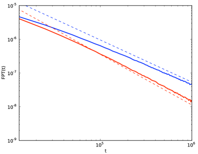
Figure 4: (color online) FPT densities for the comb (upper curve, blue) and for the RWRW (lower curve, red). The dashed lines give the theoretical asympototic behaviours.

Another fundamental intrinsic characteristic is the auto-correlation function. Let $s_{i}$ be the $i$-th step of the walker, so that $x_{n}=\sum_{i=0}^{t}s_{i}$. The MSD is therefore:

$$\left\langle x^{2}_{n}\right\rangle=\left\langle\sum_{i,j=0}^{t}{s_{i}s_{j}}\right\rangle=\sum_{i,j=0}^{t}C_{ij},$$ (16)

where the average is taken over different realizations and $C_{ij}=\langle s_{i}s_{j}\rangle$ is the step-step correlation function.

Here the stationary, ergodic RWRW model differs crucially from the non-stationary CTRW one, since for stationary RWRW processes $C_{ij}$ only depends on the difference of its arguments $C_{ij}=C_{|i-j|}$ and is an oscillating, slowly decaying function (vide infra). On the other hand, for CTRW different steps along the backbone of the comb are uncorrelated, so that $C(i,j)=M(i)\delta_{i,j}$ with $M(i)$ being the probability that the time-step $t=i$ corresponds to a step on the backbone and not on a tooth, i.e. to the rate of relevant steps. This one can be evaluated via $\chi(n,t)$ Klafter and Sokolov (2011) and for large $t$ behaves as $M(t)\simeq(2\pi)^{-1/2}\;t^{-1/2}$. The explicit dependence of $C(i,j)$ on time is a fingerprint of the non-stationarity of CTRW.

To asses $C_{\tau}=\left\langle s_{n}s_{n+\tau}\right\rangle$ for a RWRW we have to look separately at even and odd time lags $\tau=|i-j|$. The first step $s_{n}$ of the RW corresponds to zero delay and is taken to be in a positive direction along the track (to the right). Since the track of the RW is an uncorrelated RW itself, the two steps are correlated only if they correspond to the motion over the same step (bond) of the track, so that $s_{n}s_{n+\tau}=\pm 1$ depending whether the bond is crossed in the same direction (at even lags) or in the opposite directions (at odd lags), and are uncorrelated otherwise. Crossing of the same bond takes place with probability 1/2 and only if the walker was at its starting position (even lags) or at its position after performing the first step (odd lags). For $\tau=2k$ the probability that the RW on a track returns to its starting point is given by the binomial distribution $\mathrm{binom}(k,2k-1,1/2)$ (where $\mathrm{binom}\left(k,n,p\right)=\frac{n!}{k!(n-k)!}p^{k}(1-p)^{n-k}$). For $\tau=2k+1$ the return to the endpoint of the first step takes place with the probability $\mathrm{binom}(k,2k,1/2)$. We therefore have $C_{0}=1$ and $C_{1}=-1/2$, and generally:

$$C_{2k}=(1/2)\mathrm{binom}\left(k,2k-1,1/2\right)$$

$$C_{2k+1}=(-1/2)\mathrm{binom}\left(k,2k,1/2\right).$$ (17)

Thus a RWRW model is a bona fide anti-persistent RW model. Eq. (The Unequal Twins - Probability Distributions Aren’t Everything) has been numerically verified.

Note that both correlation functions, the one for RWRW and the one for the comb, lead to the same MSDs. For RWRW we have: $\left\langle x^{2}_{n}\right\rangle=2\sum_{k=0}^{n}(n-k)C_{k}-C_{0}-C_{n}$. For large $t=n$ the two last contributions $C_{0}=1$ and $C_{n}\to 0$ can be neglected compared to the sum and $C_{k}$ can be approximated via the Stirling formula giving $C_{k}=\pm(2\pi k)^{-1/2}$. Passing from the sum to the integral we get for large $n$ $\left\langle x^{2}_{n}\right\rangle=\sqrt{2\pi^{-1}}n^{1/2}$. For the comb we get $\left\langle x^{2}_{n}\right\rangle=\sum_{k=1}^{n}(2\pi)^{-1/2}\;k^{-1/2}\approx\int_{0}^{n}\sqrt{2/\pi}\;k^{-1/2}dk=\sqrt{2\pi^{-1}}n^{1/2}$, same as above.

Let us summarize our findings. We discussed the behavior of two popular models of geometrically induced subdiffusion: the random walk on a comb (the model of the CTRW class) and the random walk on the random walk’s trajectory, belonging to the class of anti-persistent random walks. Although both models lead to exactly the same PDFs at all times, they are crucially different with any other respect like FPTs or correlation functions, which mirror the fact that the RWRW model is stationary and the CTRW model is not.

The difference in these behaviors leads us to a following conclusion. We say that a model is described by some equation if several relevant properties of the model can be obtained by solving this equation with corresponding initial and boundary conditions. For example, the fractional diffusion equation describes the comb model because not only the Green’s function (PDF $p(x,t)$, the solution for free boundaries), but also the FPT distribution to the point $x_{1}$ follows from the corresponding equation, now with the boundary condition $p(x_{1},t)=0$. This is definitely not the case for the RWRW model, for which we have to admit that the knowledge of the Green’s function (and of the equation for it) is not enough to obtain the FPT, and the model is not fully described by this equation. Any conclusions about the nature of the process based on the PDF (or moments) alone or on the knowledge of the equation for such a PDF may thus stand on a quite shaky basis.

I Supplementary Material

I.1 MSD of the comb model

Let us define the total number of time steps as $n$ and the number of steps taken in the $x$-direction as $n_{x}$. The number of steps taken in the $y$-direction is then $n_{y}=n-n_{x}$. Using CTRW arguments Metzler and Klafter (2000) and given that the distribution of soujourn times in the teeth is given by $\psi(t)\simeq\frac{1}{\sqrt{2\pi}}t^{-3/2}$, the one-dimensional ensemble MSD along the backbone takes the form:

$$\langle x^{2}\rangle_{ens}\sim\langle n_{x}\rangle\sim n^{1/2}.$$ (18)

Similarly, for the $y$-axis we have:

$$\langle y^{2}\rangle_{ens}\sim\langle n_{y}\rangle=\langle n-n_{x}\rangle=n-n^{1/2}.$$ (19)

The two-dimensional MSD is then the sum of the two one-dimensional MSDs, resulting in a linear time dependence:

$$\langle r^{2}\rangle=\langle x^{2}\rangle+\langle y^{2}\rangle=n.$$ (20)

This result is numerically verified, displayed in the inset of Fig. 3 in the main text.

One should note that one commonly treats the motions in the $x$ and $y$ directions as independent Sokolov and Eliazar (2010a); Weiss (1994) which leads to a two-dimensional propagator being the product of the two one-dimensional propagators. This, in turn, leads to a two-dimensional MSD non-linear in time, the one behaving as

$$\langle r^{2}\rangle_{ens}=\langle x^{2}\rangle_{ens}+\langle y^{2}\rangle_{ens}\sim n^{1/2}+n.$$ (21)

Although this is asymptotically linear, the numerics in Fig. 3 from the main text clearly exhibit a completely linear time dependence at all time scales including the shortest ones, thus rejecting this view in favour of the one presented above.

Eq. 20 describes normal diffusion on the comb structure, which, contrary to the diffusion in the projection on the $x$-direction, is a stationary and ergodic random process. We also note that a random walk on a percolation cluster at criticality is subdiffusive, meaning that the comb structure is inherently inadequate to model a percolation cluster.

I.2 The FPT distributions

Let us obtain the FPT distribution of the RWRW model, again by averaging over the initial point and the realizations of the walk. We fix the starting point $x=0$ and the final point $x_{1}$. The RW trajectory on which the random walk than takes place has two strands connecting these two points (since in 1D a RW is certain to reach any given point on a line), and therefore the corresponding random walk takes place on a finite interval. The distances $l_{1}$ and $l_{2}$ along the corresponding strands are independent random variables, both distributed according to the Smirnov law

$$f(l_{1,2}|x)=\frac{x}{2\sqrt{\pi}l_{1,2}^{3/2}}\exp\left(-\frac{x^{2}}{4l_{1,2}}\right).$$ (22)

Therefore the corresponding RW on the RW takes place at an interval $(-l_{1},l_{2})$ starting at $l=0$, or, equivalently, on an interval of length $L=l_{1}+l_{2}$ starting at a point at a distance $l_{1}$ from the left boundary of the interval. It is convenient to change the variables, and to consider a symmetric interval $(-L/2,L/2)$ with the starting point $y=(l_{1}-l_{2})/2$ inside it (being at the distance $l_{1}$ from its left boundary and at the distance $l_{2}$ from the right one). The probability to find a particle at position $l$ within this interval with absorbing boundaries (in the diffusion approximation, $D=1/2$) is given by

$$P(l,t)=\frac{2}{L}\sum_{m=0}^{\infty}\cos\left(b_{m}l\right)\cos\left(b_{m}y\right)\exp{(-b_{m}^{2}Dt)},$$ (23)

where $b_{m}=\pi(2m+1)/L$. Integration over $l$ gives us the survival probability

$$\Phi_{1,2}(t)=\sum_{m=0}^{\infty}(-1)^{m}\frac{4}{Lb_{m}}\cos\left(b_{m}y\right)\exp{(-b_{m}^{2}Dt)}$$ (24)

which has to be averaged over the position of the starting point $y$ and of the length of the interval. The overall explicit evaluation of the mean of this series is tedious, but finding the long time asymptotic behavior is relatively simple. To do this, we note that at long times only the first term ($m=0$) plays a role, so that

$$\Phi_{1,2}(t)\approx\frac{4}{\pi}\cos\left(\frac{\pi y}{2L}\right)\exp{\left(-\frac{\pi^{2}}{L^{2}}Dt\right)},$$ (25)

where $Dt=n/2$. The average over the position of the starting point $y$ and of the length of the interval is given by:

$$\Phi(t)=\iint\limits^{\>\>\>\>\>\>\>\>\infty}_{0}\Phi_{1,2}(t)p(l_{1})p(l_{2})\mathrm{d}l_{1}\mathrm{d}l_{2}.$$ (26)

We substitute Eqs. (25) and (22) in Eq. (26) and make a change of variables, $L=l_{1}+l_{2}$ and $z=l_{2}/l_{1}$ (the Jacobian of this transformation is $\partial(l_{1},l_{2})/\partial(L,z)=L/(1+z)^{2}$). Making a further transformation, $\xi=1/L$, leads to

$$\Phi(t)=\frac{x^{2}}{\pi^{2}}\iint\limits^{\>\>\>\>\>\>\>\>\infty}_{0}\frac{1+z}{z^{3/2}}\cos(\frac{\pi}{2}\frac{1-z}{1+z})e^{(-\pi^{2}Dt\xi^{2}-\frac{x^{2}(1+z)^{2}}{4z}\xi)}\mathrm{d}\xi\mathrm{d}z.$$ (27)

We are interested in the asymptotic behavior of this function for $t\to\infty$. The integral over $\xi$ can be taken in quadratures:

$$I_{1} = \int_{0}^{\infty}\exp\left(-\pi^{2}Dt\xi^{2}-\frac{x^{2}(1+z)^{2}}{4z}\xi\right)d\xi$$

$$= \frac{1}{2\sqrt{\pi Dt}}\exp\left(\frac{x^{4}(1+z)^{4}}{64z^{2}\pi^{2}Dt}\right)\mathrm{erfc}\left(\frac{x^{2}(1+z)^{2}}{8z\pi\sqrt{Dt}}\right)$$

and tends to

$$I_{1}\to\frac{1}{2\sqrt{\pi Dt}}$$ (28)

for $t\to\infty$ (unless $z$ gets extremely large, when it starts to decay as $z^{-1}$). Such large values of $z$ do not play any role, since the integral

$$I_{2}=\int_{0}^{\infty}\cos\left(\frac{\pi}{2}\frac{1-z}{1+z}\right)\frac{1+z}{z^{3/2}}dz$$ (29)

converges: It is equal to $\,{}_{1}F_{2}\left(1,\frac{1}{2},\frac{3}{2},-\frac{\pi^{2}}{16}\right)$ where $\,{}_{1}F_{2}$ is the generalized hypergeometric function (the integral can be transformed to the form (Eq. 2.5.8.1 in Prudnikov et al. (1988)) by the change of variable $y=(1-z)/(1+z)$ ). The numerical evaluation of the integral gives approximately the value $I_{2}=11.2$. This numerical evaluation results in the survival probability whose asymptotical behaviour at $t\rightarrow\infty$ follows:

$$\Phi(t)\simeq C\frac{x^{2}}{\sqrt{Dt}},$$ (30)

where $C=I_{2}/(2\pi^{5/2})\approx 0.64$.

I.3 Marginal distributions for the RWRW

For the sake of completeness we give here the expression for $P(L,z)$, the joint probability density that a point on a track chosen at random falls in the interval of length $L$ between its two crossing points with the $x=const$ line and divides this interval into two parts whose length quotient is $l_{1}/l_{2}=z$. This one is obtained by the variable transformation from $p(l_{1},l_{2})=p(l_{1}|x)p(l_{2}|x)$ with $p(l|x)$ given by Eq. (22) and reads

$$P(L,z)=\frac{x^{2}}{4\pi}\frac{1+z}{z^{3/2}}\frac{1}{L^{2}}\exp\left(-\frac{(1+z)^{2}}{z}\frac{x^{2}}{4L}\right).$$ (31)

The marginal distribution in $z$ follows elementary Sokolov and Eliazar (2010b):

$$p(z)=\int_{0}^{\infty}P(L,z)dL=\frac{1}{\pi}\frac{1}{\sqrt{z}(1+z)}.$$ (32)

This distribution corresponds to a very uneven distribution of the starting point within the interval (the equidistribution would correspond to $p(z)=(1+z)^{-2}$, and doesn’t have a singularity at small $z$). This means, that in our case the particle starts close to one of the ends of the interval (the distributions of $z$ and $1/z$ are the same), and therefore the FPT distribution decays faster than in the case of the equidistribution.

To calculate the marginal distribution in $L$, one first passes to the distribution of the variable $\xi=1/L$:

$$P(\xi,z)=\frac{x^{2}}{4\pi}\frac{1+z}{z^{3/2}}\exp\left(-\frac{(1+z)^{2}}{z}\frac{x^{2}}{4}\xi\right),$$ (33)

takes the Laplace transform in $\xi$ to obtain

$$\tilde{P}(u,z)=\frac{1}{\pi}\frac{x^{2}(1+z)}{\sqrt{z}(4uz+x^{2}(1+z)^{2})},$$ (34)

performs integration in $z$ (which is an elementary but tedious procedure) to obtain

$$\tilde{p}(u)=\int_{0}^{\infty}\frac{1}{\pi}\frac{x^{2}(1+z)}{\sqrt{z}(4uz+x^{2}(1+z)^{2})}dz=\frac{x}{\sqrt{u+x^{2}}}$$ (35)

takes the inverse Laplace transform,

$$p(\xi)=\frac{x}{\sqrt{\pi\xi}}\exp(-x^{2}\xi)$$ (36)

and finally returns to $L$ to get

$$p(L)=\frac{1}{\sqrt{\pi}L^{3/2}}\exp\left(-\frac{x^{2}}{L}\right),$$ (37)

the Smirnov distribution, as anticipated.

Note that neglecting the role of the initial position (which, as stated, is extremely unevenly distributed within the $L$-interval) would lead to a different result, namely to:

$$\Phi(t)=\frac{x}{2\pi^{3/2}\sqrt{Dt}}e^{\left(\frac{x^{4}}{8\pi^{2}Dt}\right)}K_{1/4}\left(\frac{x^{4}}{8\pi^{2}Dt}\right)$$ (38)

(see Eq. 2.3.15.5 in  Prudnikov et al. (1988)). Using the behavior of the modified Bessel functions for small values of its argument, $K_{1/4}(z)\simeq\frac{1}{2}\Gamma(1/4)(z/2)^{-1/4}$ (see Eq. 9.6.9 in Abramovitz and Stegun (1964)) we would get that $\Phi(t)\propto t^{-1/4}$ like in the CTRW.

References

- Weiss and Havlin (1986) G. H. Weiss and S. Havlin, Physica A 134, 474 (1986).
- Kehr and Kutner (1982) K. W. Kehr and R. Kutner, Physica A 110, 535 (1982).
- Doi and Edwards (1988) M. Doi and S. F. Edwards, The Theory of Polymer Dynamics (Oxford Science Press, 1988).
- Metzler and Klafter (2000) R. Metzler and J. Klafter, Physics Reports 339, 1 (2000).
- Chandrasekhar (1943) S. Chandrasekhar, Rev. Mod. Phys. 15, 89 (1943).
- Klafter and Sokolov (2011) J. Klafter and I. M. Sokolov, First Steps in Random Walks (Oxford University Press, Oxford, 2011).
- Sokolov et al. (2001a) I. M. Sokolov, A. Blumen, and J. Klafter, Europhysics Letters 56, 175 (2001a).
- Sokolov et al. (2001b) I. M. Sokolov, A. Blumen, and J. Klafter, Physica A: Statistical Mechanics and its Applications 302, 268 (2001b).
- (9) For a detailed calculation we refer to the Supplementary Material.
- Meroz et al. (2011) Y. Meroz, I. M. Sokolov, and J. Klafter, Phys. Rev. E 83, 020104 (2011).
- Sokolov and Eliazar (2010a) I. M. Sokolov and I. I. Eliazar, Phys. Rev. E 81, 026107 (2010a).
- Weiss (1994) G. H. Weiss, Aspects and Applications of the Random Walk (North Holland Press, Amsterdam, 1994).
- Prudnikov et al. (1988) A. Prudnikov, Y. Brychkov, and O. Marichev, Integrals and Series (Gordon & Breach Science Publishers/CRC Press, 1988).
- Sokolov and Eliazar (2010b) I. Sokolov and I. Eliazar, Phys. Rev. E 81, 026107 (2010b).
- Abramovitz and Stegun (1964) M. Abramovitz and I. Stegun, Handbook of Mathematical Functions (Dover, 1964).