Cloud Modeling of a Network Region in H$\alpha$

Abstract

In this paper, we analyze the physical properties of dark mottles in the chromospheric network using two dimensional spectroscopic observations in H$\alpha$ obtained with the Göttingen Fabry-Perot Spectrometer in the Vacuum Tower Telescope at the Observatory del Teide, Tenerife. Cloud modeling was applied to measure the mottles’ optical thickness, source function, Doppler width, and line of sight velocity. Using these measurements, the number density of hydrogen atoms in levels 1 and 2, total particle density, electron density, temperature, gas pressure, and mass density parameters were determined with the method of Tsiropoula & Schmieder (1997). We also analyzed the temporal behaviour of a mottle using cloud parameters. Our result shows that it is dominated by 3 minute signals in source function, and 5 minutes or more in velocity.

1 Introduction

The main fine structures of the quiet chromosphere emanating from the network are called mottles when seen on the disk and spicules when seen at the limb. Mottles appear as dark or bright structures, which together form two kinds of groups, namely rosette and chain. The mottles in a rosette spread radially outwards from a bright center, while in a chain they all point in the same direction. The dark mottles are thin and elongated structures, whereas the bright mottles are small and roundish, lying at a lower height than the dark ones. These structures presumably extend along the magnetic fields and cover between $7^{\prime\prime}$ and $10^{\prime\prime}$ with widths smaller than $1^{\prime\prime}$ and have lifetimes of the order of 10 min or more. The spatial relationship between the bright and dark mottles is given in detail by Zachariadis et al. (2001) (see also references therein).

There are a number of studies on the physical properties of chromospheric fine structures using spectrometric observations as well as various theoretical models and simulations (Sterling 2000; Tziotziou et al. 2003; Al et al. 2004; De Pontieu et al. 2004; Rouppe van der Voort et al. 2007). Assuming an optically thin absorbing cloud in front of a radiation source, the standard cloud model (Beckers 1964) has been extensively used to extract intrinsic line formation parameters such as source function, optical thickness, Doppler width and line of sight velocity (see review by Tziotziou 2007).

In this paper, we analyzed chromospheric features observed in H$\alpha$ line with very good spectral profile sampling to derive the features’ physical properties in terms of standard cloud modeling. Using the method of Tsiropoula & Schmieder (1997), additional physical parameters were also derived from the inferred cloud model parameters. We also addressed the dynamics of a dark mottle by the analysis of cloud velocity and source function variations. Our goal is to define the physical conditions inside dark mottles and to investigate the oscillatory behaviour by taking advantage of high resolution imaging spectroscopic capabilities of the Göttingen Fabry-Perot spectrometer and comparing our results with previous studies.

2 Observations and Data Analysis

The data were obtained with the Vacuum Tower Telescope (VTT)’s Göttingen Fabry-Perot spectrometer, which is based on two Fabry-Perot Interferometers (Koschinsky et al. 2001). In 2002, a short time series of 60 wavelength scans of the H$\alpha$ line were taken from a network region near the disk center of the sun. A spacing of 125 mÅ  between adjacent wavelength positions was chosen for the spectral scans. With the narrow-band channel, 8 images at each of 18 wavelength positions were obtained, which provides a wavelength coverage of approximately 2.125 Å. The exposure time was 30 ms and the time interval between the start of two subsequent spectral scans was 49 s. The observed field of view of the raw data was $38^{\prime\prime}.4\times 28^{\prime\prime}.6$, with a spatial scale of $0^{\prime\prime}.1$ per pixel. During the observations obtained under good seeing conditions, broad-band images were taken simultaneously with narrow-band images. Our best scan reached a Fried parameter of r₀=21 cm. Dark scans, flat fields and scans with the continuum source were also taken for the data reduction.

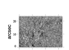
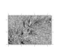
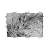
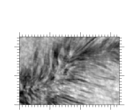
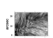
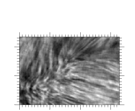
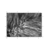
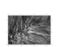
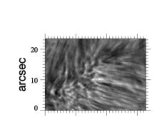
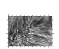
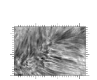
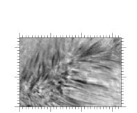
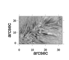
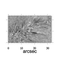
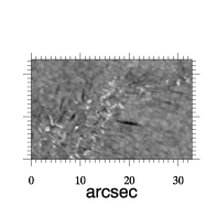
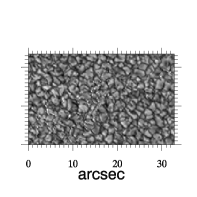
Figure 1: A sample of speckle reconstructed narrow-band scan and the broad-band image (lower right) belonging to the same field of view. The size of each image is $32^{\prime\prime}\times\,23^{\prime\prime}.6$. The wavelength positions decrease in each image by 125 mÅ  starting from 6563.8  Å  at the upper-left corner. The last image in the second row is the closest to the center of the line profile.

Broad-band images were restored by using the spectral ratio (von der Lühe 1984) and the speckle masking technique (Weigelt 1977). Narrow-band images were reconstructed by using Keller and von der Lühe’s (1992) method.

As a result of this method, we obtained one reconstructed narrow-band image for each wavelength position of the H$\alpha$ line. Figure 1 displays the reconstructed narrow-band images through one scan. The observed region contains almost parallel elongated dark mottles, which form the so-called ’chains of mottles’.

For each pixel in the field of view, H$\alpha$ line profiles were constructed from intensity values of narrow band images obtained at 18 wavelength positions.

3 The Cloud Model

The shapes and amplitudes of stellar spectral line profiles reflect the physical properties of the regions they are formed in. Therefore, physical parameters such as chemical abundance, density, temperature, velocity, magnetic field, micro-turbulence, etc. of these regions can be inferred through the analysis of observed spectral line profiles.

The standard cloud model (Beckers, 1964) has been used extensively to determine the physical properties of solar chromospheric fine structures. The model considers a chromospheric feature like a cloud above a uniform atmosphere described by a reference background profile. The approach works well for optically thin structures and gives estimates of source function $S$, optical thickness at the line center $\tau_{0}$, Doppler width $\Delta\lambda_{\rm D}$, and line-of-sight velocity $v_{\rm LOS}$ for the observed cloud. These parameters are assumed to be constant within the cloud along the line of sight. The observed contrast profiles are matched with the theoretical contrast profiles using the following formula

$$C(\lambda)={{I(\lambda)-I_{0}(\lambda)}\over{I_{0}(\lambda)}}=\left({S\over{I_{0}(\lambda)}}-1\right)(1-e^{{-}\tau(\lambda)})$$ (1)

where I${}_{0}(\lambda)$ is the reference profile emitted by the background and $\tau(\lambda)$ is the optical thickness. The wavelength dependence of optical thickness is given by

$$\tau(\lambda)=\tau_{0}\exp\left[-\left({\lambda-\lambda_{c}(1-\upsilon_{LOS}/c)\over\Delta\lambda_{D}}\right)^{2}\right]$$ (2)

where $\lambda_{c}$ is the line center wavelength and $c$ is the speed of light. The standard cloud model considers chromospheric fine structures to be completely isolated from the surrounding atmosphere and illuminated from the underlying atmosphere.

The result of the cloud modeling is based on fitting the observed contrast profile with the model from an iterative least square procedure for non-linear functions. The line core intensity and the line core position of the observed profile were taken respectively as initial values of $S$ and $\lambda_{c}$ for the iteration procedure. For $\tau_{0}$ and $\Delta\lambda_{\rm D}$ the values 1 and 0.3 Å were used.

In order to determine the physical parameters of dark mottles using the cloud model, we selected dark features in the field of view by masking pixels greater than 0.9 of mean value of the line center intensity image for each spectral scan. Then we constructed line profiles for each selected pixel and calibrated them relative to the quiet sun continuum. Finally, we calculated a contrast profile for each selected pixel using the mean of all profiles in the field of view as the background profile and applied the cloud model.

4 Results and Discussion

4.1 Results of Cloud Modelling

Figure 2 displays histograms of cloud parameters inferred for all the time series for dark mottles. The source function distribution shows a peak near 0.11 (in units of the continuum intensity $I_{c}$), while the Doppler width’s peak is close to 0.46 Å. The peak of the optical thickness distribution is around 0.8, which indicates that dark mottles are mostly optically thin structures. The distribution of line-of-sight velocities varies between $-$30 and 30 km s^-1, and is almost symmetric, which implies the presence of both downward and upward motions. It peaks around $-$1.25 km s^-1 (downward).

Figure 2: Distribution of cloud parameters. Negative values indicate a downward motion in the line-of-sight velocity.

Figure 3 shows maps of the cloud model parameters obtained for one scan. The map of source function has minimum values at the center regions of individual dark mottles. Through the edge of the structures, the source function values are close to the line center intensity of the background profile. We observe that regions of high Doppler width values have low optical thickness and vice versa. This anticorrelation was also noticed by Alissandrakis et al. (1990) and Tsiropoula et al. (1993). On the map of the Doppler shift, downflows and upflows are always present along mottles while material is mostly descending near their footpoints.

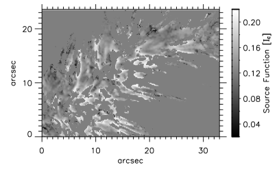
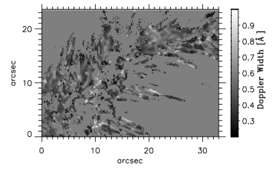
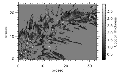
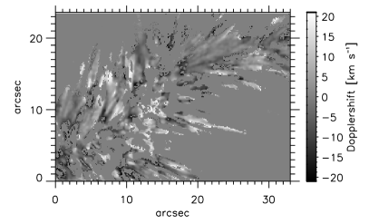
Figure 3: Maps of the source function, Doppler width, optical thickness at the line center and line of sight velocity. In the medium grey areas either the cloud model fit was not applied or did not give meaningful results at all. In the Doppler shift map, the bright and dark patches indicate upflows and downflows, respectively.

Table 1 shows values of the cloud parameters reported by various authors. It can be seen from the table that our results, inferred for all the time series are in good agreement with previous measurements. Several intrinsic parameters can be determined by using the cloud model parameters. Assuming 15 km s^-1 for microturbulent velocity, $\xi_{t}$, we can calculate temperature from the deduced Doppler width values;

$$\Delta\lambda_{D}={\lambda_{0}\over c}\sqrt{{2kT\over m_{H}}{+\xi^{2}_{t}}}$$ (3)

The relation between the optical thickness at the line center, the Doppler width and the number density in the second hydrogen level $N_{2}$ may be given:

$$\tau_{0}={\pi^{1\over{2}}e^{2}\over{m_{e}c}}{f\lambda^{2}\over{c}}{N_{2}L\over\Delta\lambda_{D}}{d}$$ (4)

inserting the constants in the equation above, we obtain:

$$\tau_{0}=1.38\times 10^{21}{N_{2}d\over\Delta\lambda_{D}}$$ (5)

The thickness of mottles estimated at the images was assumed to $\approx$350 km, considering a cylindrical structure, and the inclination was taken as $\approx$30^∘ given for spicules by Heristchi and Mouradian (1992). Therefore the geometrical width, $d$ of the structures under investigation, is equal to $\approx$700 km. Then using the same method as Tsiropoula & Schmieder (1997), we also obtained the electron density $N_{\rm e}$, the total particle density $N_{\rm H}$, the gas pressure $p$, the total column mass $M$, the mass density $\rho$, and the degree of hydrogen ionization $\chi_{\rm{H}}$. The relations can be expressed as:

$$N_{\rm e}=3.2~{}10^{8}\sqrt{N_{2}}$$ (6)

$$N_{\rm H}=5~{}10^{8}~{}10^{0.5~{}\log N_{2}}$$ (7)

$$p=k(N_{\rm e}+1.0851~{}N_{\rm H})~{}T$$ (8)

$$M=(N_{\rm H}m_{\rm H}+0.0851~{}N_{\rm H}\times 3.97m_{\rm H})~{}d$$ (9)

$$\rho={M\over d}$$ (10)

and

$$\chi_{\rm H}={N_{\rm e}\over N_{\rm H}}$$ (11)

We assumed histograms of the parameters to be normally distributed, so we fit them with a Gaussian curve separately. We took peak values of Gaussian distributions as a mean value and their 1$\sigma$ widths as a standard error. In Table 2, we present the results obtained from all the time series and compare these with the values found by Tsiropoula & Schmieder (1997) and Tsiropoula & Tziotziou (2004) for dark mottles. The results are generally in agreement with previous computations, although some variations do exist. These differences may arise from various factors. First, the atmospheric seeing when the observation was performed, has a non-negligible effect on the determination of cloud parameters, especially on the Dopplerwidth (Tziotziou et al., 2007). Therefore, it causes an uncertainty in the calculation of the pressure and temperature, which depends on the Dopplerwidth and the microturbulent velocity, which is assumed. Second, any uncertainties raised at the determination of the geometrical thickness of the structures, $d$, will be propagated to the uncertainties in the calculations of $N_{2}$, $N_{\rm e}$ and $M$. Finally, differences in the inferred values of $\tau_{0}$ can cause variations in these parameters.

Table 1: Cloud model parameters for dark mottles given by different authors.

Authors	$S$	$\upsilon$ (km s-1)	$\tau_{0}$	$\Delta\lambda_{D}$ (Å)
Beckers 1968	123	-	1.4	0.5
Bray 1973	130 to 160	-9 to 7	1.0	0.5
Grossmann-Doerth $\&$	130	-8 to 8	1.1	0.45
von Uexküll 1977
Tsiropoula et al. 1993	163.3$\pm 14.3$	-0.26$\pm 6.6$	1.8$\pm 1.1$	0.37$\pm 0.1$
Lee et al. 2000	0.16 $I_{c}$	-2.8	2.2$\pm 0.5$	0.55
Tziotziou et al. 2003	0.15  $I_{c}$	-0.1	0.9	0.35
Al et al. 2004	0.14  $I_{c}$	0.18	1.58	0.44
This work	0.11 $I_{c}$	-1.25	0.8	0.46

Table 2: Pyhsical parameters for dark mottles given by different authors.

Parameters	Tsiropoula & Schmieder	Tsiropoula & Tziotziou	This work
	(1997)	(2004)
$N_{1}(cm^{-3})$	$(1.6\pm 0.8)10^{10}$	$-$	$(3.0\pm 0.7)10^{10}$
$N_{2}(cm^{-3})$	$(1.4\pm 1.1)10^{4}$	$(4.2\pm 2.0)10^{4}$	$(4.2\pm 1.9)10^{4}$
$N_{e}(cm^{-3})$	$(3.4\pm 1.5)10^{10}$	$(6.4\pm 1.6)10^{10}$	$(7.0\pm 1.6)10^{10}$
$N_{H}(cm^{-3})$	$(5.1\pm 2.1)10^{10}$	$(9.9\pm 2.5)10^{10}$	$(10.8\pm 2.5)10^{10}$
$T(K)$	$(1.0\pm 0.8)10^{4}$	$(1.0\pm 0.3)10^{4}$	$(1.2\pm 0.9)10^{4}$
$P(dyn~{}cm^{-2})$	$0.15\pm 0.1$	$0.24\pm 0.1$	$0.32\pm 0.2$
$M~{}(gr~{}cm^{-2}$)	$(2.2\pm 0.4)10^{-5}$	$(2.2\pm 0.6)10^{-5}$	$(1.6\pm 0.4)10^{-5}$
$\rho~{}(gr~{}cm^{-3}$)	$(1.1\pm 0.5)10^{-13}$	$(2.2\pm 0.6)10^{-13}$	$(2.4\pm 0.6)10^{-13}$
$\chi_{\rm{H}}$	0.65$\pm$0.1	0.65	$0.64\pm 0.1$

We calculated the pressure inside the dark mottles as 0.32 dyn cm^-2. This result is in agreement with Heinzel & Schimieder (1994), who concluded that classical cloud model can be applied to low pressure structures ($<$ 0.5 dyn cm^-2), assuming a constant source function and a rather low opacity.

Previous studies of spicules show that they have temperatures of about 5 000-15 000 K, and densities of about 3$\times$10^-13 g cm^-3. The physical properties we inferred from cloud modeling here for the mottles are in good agreement with the values found earlier for the spicules showing further evidence that these two features have significant similarities (Table 2).

4.2 Temporal Analysis of a Mottle

In order to study the oscillatory behaviour of chromospheric features, we performed a Fourier analysis to the fluctuations of cloud model’s source function and Dopplershift for a long horizontal mottle’s region. This region which is centered at (8, 8) is shown with a white rectangle in Figure 4. We selected this region because it could be well isolated from other structures and the cloud model fit it well for all of the time series.

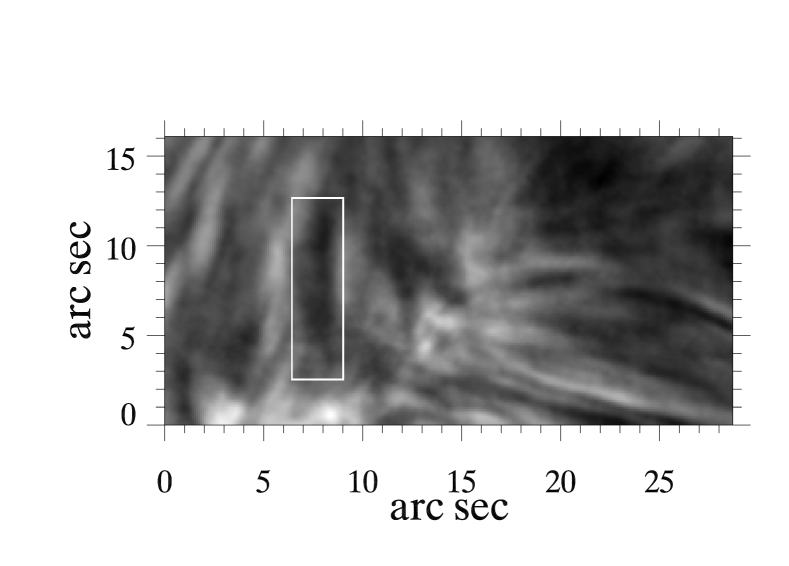
Figure 4: The mean image of H$\alpha$ line center intensity series (top). White rectangle inside the image marks the mottle selected for the Fourier analysis. The distribution of optical thickness for the mottle subjected to timing analysis. (bottom).

Figure 5: Power spectra for the cloud source function and Dopplershift fluctuations of the mottle (top and bottom, respectively).

Before computing the power spectra, we averaged the signal in the selected mottle’s region and then applied a polynomial trend removal of the 4th order to the time series of source function and velocity. Consequently, we cut down the power at frequencies lower than 0.7 mHz, which corresponds to half of the total duration of our observation. This procedure also affected the amplitude of the power at the frequencies lower than 1.3 mHz, but the power at high frequencies remained unaffected.

In Figure 5, we show the power spectra of Cloud Dopplershift and source function variations in the considered mottle’s region. Power distribution of source function peaks at high frequencies between 5 and 8 mHz with a maximum around 5.7 mHz (i.e periods of 3 minutes) which corresponds to the acoustic cut-off frequency. The second significant power with a lower amplitude is around 7.2 mHz. De Pontieu et al. (2007) also reported a significant 3 minute periodicity in the intensity variations of the overlying loops emanating from a network. They considered that the lower opacity of these structures allows glimpses of internetwork dynamics and oscillations underneath. In order to check this scenario, we looked into the distribution of optical thickness for the considered mottle (Figure 4). The peak is around 0.6, which is smaller than the peak of general distribution of optical thickness presented in Figure 2. This shows that the long mottle under consideration has a lower opacity and also confirms the suggestion of De Pontieu et al. (2007). In the power spectrum of source function, significantly lower powers are seen at low frequencies around 2.2 and 3.5 mHz.

The cloud Dopplershift power spectrum shows three well separated peaks at lower frequencies. The most significant peak lies around 2.2 mHz, i.e. at periods of 7 minutes. The other two are around 1.3 mHz and 3.5 mHz (i.e periods of 5 minutes). We should note that magnitude of the power around 1.3 mHz is strongly affected by the procedure of trend removal, so we can not form a conclusion about its relevance. Also, peaks in the 3 minute range are visible but they have remarkably less significance.

Similar to our results for the periodicities in velocity variations, Tziotziou et al. (2004) found a dominant period in the 5 minutes (3.3 mHz) for intensity and velocity variation of dark mottles. De Pontieu et al. (2007) reported that the mottles are dominated by oscillatory behavior with periods around 5 minutes and longer. More recently, Tsiropoula et al. (2009) found a significant peak around the 5 minute range for the mottles’ region.

This strong peak around 5 minutes which was observed in the Doppler velocity power spectrum has long been attributed to p-mode oscillations generated at the photosphere propagate upward in and around magnetic flux concentrations of a network (Giovanelli et al. 1978). Several studies based on simulations and observations have suggested that low frequency ($<$5 mHz) magnetoacoustic waves might propagate into the chromosphere along magnetic field lines which are significantly inclined with respect to the surface gravity (Bel & Leroy 1977; Suematsu 1990; De Pontieu et al. 2004; Jefferies et al. 2006). In order to study the propagation characteristics of waves at different heights in atmosphere, it is essential to compute phase difference and coherence spectra. In a future paper, we will concentrate on this issue in detail using the lambdameter method (Tsiropoula et al., 1993; Al et al., 2004) to compute intensity and Dopplershift image series for different widths through the H$\alpha$ profile.

In this work, using high spectral and spatial resolution spectro-imaging observations, we constructed H$\alpha$ line profiles for every pixel of mottles in the field of view. We fit the resulting profiles with the cloud model and infered physical parameters of the dark mottles, which agree with previous studies. We also performed a Fourier analysis on fluctuations of the cloud velocity and source function to detect the oscillatory behaviour of the mottles. However, we could only concentrate on one mottle in the field of view since the cloud model can not fit the all of the profiles. Our analysis shows that the mottle is dominated by 3 minute periods (the acoustic cut-off period in the chromosphere) in source function, and periods of 5 minute and longer in Dopplershift.

- [1] Al, N., Bendlin, C., Hirzberger, J., Kneer, F., Trujillo Bueno, J.: 2004, A&A 418, 1131
- [2] Alissandrakis, C.E., Tsiropoula, G., Mein, P.: 1990, A&A 230, 200
- [3] Beckers, J.M.: 1964, Ph.D. Thesis, Utrecht
- [4] Beckers, J.M.: 1968, Sol.Phys. 3, 367
- [5] Bel, N. & Leroy, B. 1977, A&A, 55, 239
- [6] Bray, R.C., 1973, Sol.Phys. 29, 317
- [7] De Pontieu, B., Erdlyi, R., James, S. P. 2004, Nature 430, 536
- [8] De Pontieu, B., Hansteen, V. H., Rouppe van der Voort, L., van Noort, M., Carlsson, M. 2007, in Astronomical Society of the Pacific Conference Series, Vol. 368, The Physics of Chromospheric Plasmas, ed. P. Heinzel, I. Dorotovi, & R. J. Rutten, 65
- [9] Giovanelli, R. G., Harvey, J. W., & Livingston, W. C. 1978, Sol. Phys., 58, 347
- [10] Grossmann-Doerth, U., von Uexküll, M.: 1977, Sol.Phys. 55, 321
- [11] Heinzel, P., Schimieder, B., 1994, A&A 282, 939
- [12] Heristchi D., Mouradian Z., 1992, Solar Phys. 142, 21
- [13] Jefferies, S. M., McIntosh, S. W., Armstrong, J. D., et al. 2006, ApJ, 648, L151
- [14] Keller, C., von der Lühe, O.: 1992, A&A 261, 321
- [15] Koschinsky, M., Kneer, F., Hirzberger, J.: 2001, A&A 365, 588
- [16] Lee, C. Y., Chae, J., Wang, H.: 2000, ApJ 545, 1124
- [17] Rouppe van der Voort, L. H. M., De Pontieu, B., Hansteen, V. H., Carlsson, M., van Noort, M. 2007, ApJ 660, L169
- [18] Sterling, A. C. 2000, Sol. Phys., 196, 79
- [19] Suematsu, Y. 1990, in Lecture Notes in Physics, Berlin Springer Verlag, Vol. 367, Progress of Seismology of the Sun and Stars, ed. Y. Osaki & H. Shibahashi, 211
- [20] Tsiropoula, G., Alissandrakis, C. E., Schmieder, B.: 1993, A&A 271, 574
- [21] Tsiropoula, G., Schmieder, B.: 1997, A&A 324, 1183
- [22] Tsiropoula, G., Tziotziou, K.: 2004, A&A 424, 279
- [23] Tsiropoula, G., Tziotziou, K., Schwartz, P., Heinzel, P. 2009, A&A 493, 217
- [24] Tziotziou, K., Tsiropoula, G., Mein, P.: 2003, A&A 402, 361
- [25] Tziotziou, K., Tsiropoula, G., Mein, P.: 2004, A&A 423, 1133
- [26] Tziotziou, K., Heinzel, P., Tsiropoula, G.: 2007, A&A, 472, 287
- [27] Tziotziou, K.: 2007, in Astronomical Society of the Pacific Conference Series, Vol. 368, The Physics of Chromospheric Plasmas, ed. P. Heinzel, I. Dorotovi, & R. J. Rutten, 217
- [28] von der Lühe, O., 1984, J. Opt. Soc. Am. A 1, 510
- [29] Weigelt, G. P.: 1977, Optics Comm. 21, 55
- [30] Zachariadis, Th. G., Dara, H. C., Alissandrakis, C. E., Koutchmy, S., Contikakis, C.: 2001, Sol. Phys. 202, 41