Symplectic integrators with adaptive time steps

Abstract

In recent decades, there have been many attempts to construct symplectic integrators with variable time steps, with rather disappointing results. In this paper we identify the causes for this lack of performance, and find that they fall into two categories. In the first, the time step is considered a function of time alone, $\Delta=\Delta(t)$. In this case, backwards error analysis shows that while the algorithms remain symplectic, parametric instabilities arise because of resonance between oscillations of $\Delta(t)$ and the orbital motion. In the second category the time step is a function of phase space variables $\Delta=\Delta(q,p)$. In this case, the system of equations to be solved is analyzed by introducing a new time variable $\tau$ with $dt=\Delta(q,p)d\tau$. The transformed equations are no longer in Hamiltonian form, and thus are not guaranteed to be stable even when integrated using a method which is symplectic for constant $\Delta$. We analyze two methods for integrating the transformed equations which do, however, preserve the structure of the original equations. The first is an extended phase space method, which has been successfully used in previous studies of adaptive time step symplectic integrators. The second, novel, method is based on a non-canonical mixed-variable generating function. Numerical trials for both of these methods show good results, without parametric instabilities or spurious growth or damping. It is then shown how to adapt the time step to an error estimate found by backward error analysis, in order to optimize the time-stepping scheme. Numerical results are obtained using this formulation and compared with other time-stepping schemes for the extended phase space symplectic method.

1 Introduction

Adaptive time integration schemes for ODEs are well established and perform extremely well for many applications. However, for applications involving the integration of Hamiltonian systems, there are good reasons for using symplectic integrators[1]. This is particularly true in applications such as accelerators, in which very long orbits must be integrated. Symplectic integrators are also used in particle-in-cell (PIC) codes for plasma applications, where for economy integrators with lower order of accuracy must be used, but it is important that the Hamiltonian phase space structure be preserved. The same is true for molecular dynamics codes[2, 3], which are of use for dense plasmas as well as other applications. Similarly, for tracing magnetic field lines (e.g., in tokamaks or reversed field pinches) or doing RF (radio frequency) ray tracing, symplectic integrators can be very useful. To our knowledge, the symplectic integrators in use for plasma and particle beam applications all have uniform time-stepping. However, for these applications there are situations in which variable or adaptive time stepping could increase efficiency greatly. For example, in accelerators, particles can experience fields that vary over a wide range of length scales. The same is true for for PIC and MD codes, for example for particles moving in and out of shocks or magnetic reconnection layers, or undergoing close collisions.

There have been studies of symplectic integrators with variable time steps, but the early results were not promising [4, 5, 6, 7, 8, 9, 10]. Among these studies, there have been two types of variation of time steps. In the first set of studies, the time step varies with time explicitly, and in some cases varies from $\Delta t=\Delta_{1}$ to $\Delta t=\Delta_{2}$ on alternate blocks of time steps. In these studies problems were observed to arise. In the second set of studies, the time step was chosen with $\Delta t=\Delta(q,p)$, where $q,p$ are the dynamical variables. For any adaptive scheme for an autonomous system of equations, the time step is of this form. For the $\Delta(q,p)$ case, the equations are no longer in canonical Hamiltonian form (but may be Hamiltonian in non-canonical variables; see below) and indeed unfavorable results are found. The disappointing results for both of these cases have contributed to the general impression that if you need an adaptive time step integrator, you are better served using a high order non-symplectic integration method.

In this paper we take a new look at symplectic integrators with adaptive time stepping. Our focus is not on developing the most efficient or accurate symplectic integrators, but to understand and solve the problems that have been encountered in using symplectic integrators with variable time steps, and to outline a method of obtaining an optimal time-step adaptation scheme.

In Sec. 2 we start by considering time steps depending explicitly on time alone as $\Delta t=\Delta(t)=\Delta_{0}(1+\epsilon\cos\omega t)$. In Sec. 2.1 we consider several examples of first and second order symplectic integrators applied to the harmonic oscillator, and apply modified equation analysis or backward error analysis[14, 15, 11, 12]. This allows us to find the modified Hamiltonian system which the integration scheme, including the effect of numerical errors, actually solves. From this analysis we find that resonances between $\omega$ and the oscillator frequency $\Omega_{0}$ drive parametric instabilities. The resonances have $\omega=m\Omega_{0}$, the lowest order resonance having $m=2$. For first order schemes the resonance width scales as $\epsilon\Delta_{0}$, while second order schemes have width $\propto\epsilon\Delta_{0}^{2}$. These parametric instabilities explain the problematic results obtained in the papers dealing with $\Delta=\Delta(t)$[5, 7, 8, 9]. In the context of the harmonic oscillator, these problems were identified as arising from parametric instabilities by Piché[16].

We continue in Sec. 2.2 by numerically investigating time step variations $\Delta(t)=\Delta_{0}(1+\epsilon\cos\omega t)$, by integrating the harmonic oscillator with a symplectic method. We find parametric instabilities with resonance widths as predicted by the modified equation analysis. We show results of numerical integrations of a cubic oscillator with the nonlinear potential $V(q)=q^{2}/2+q^{3}/3$, in which the frequency varies with respect to the action variable, $\Omega=\Omega(J)$. The parametric instabilities seen globally for the harmonic oscillator show up as nonlinear resonances or islands, where $\omega=m\Omega(J)$, with $m$ depending on the integration method and the Hamiltonian being integrated. We observed $m=1$ islands for the cubic oscillator, integrated with the Crank-Nicolson (CN) method. The calculations of this section illustrate the point that, when considering $\Delta=\Delta(t)$, problems arise because the equations being solved become unstable (but still Hamiltonian), and not because the integration scheme fails to be symplectic.

In Sec. 3 we study time step variations $\Delta=\Delta(q,p)$. With $\Delta(q,p)\propto 1/\rho(q,p)$, the straightforward substitution $\rho(q,p)dt=d\tau$ leads to equations (having $\tau$ as the independent variable) that are not Hamiltonian equations in canonical form. Symplectic integrators therefore should not be expected to give stable results in this case, and again it has been observed that they do not. In Sec. 3.1 we review one approach to solving this problem, by extending the phase space $(q,p)\rightarrow(q,q_{0},p,p_{0})$, where $q_{0}=t$ and $p_{0}$ is its conjugate momentum. After this transformation to an extended phase space, it is easily shown that the resulting equations are Hamiltonian in canonical form and can be integrated by any fixed time step ($\Delta\tau=h=const.$) symplectic integrator in this extended phase space. This is a well-known method, and has been used to obtain symplectic integration schemes with variable time steps by Hairer[11], and also Reich[12]. Hairer described this approach as a “meta-algorithm” because any symplectic integrator can be used in the extended phase space. We then present numerical results in Sec. 3.2 for the cubic oscillator (with two different symplectic integrators) which show that, even with a step size variation that appears to have an $m=1$ resonance, evidence of non-symplectic behavior occurs and no resonant islands form.

In Sec. 3.3 we introduce a second method for dealing with the problems that arise when $\Delta=\Delta(q,p)$. The point of introducing a second method is to illustrate that the main problem with $\Delta(q,p)$ is that the equations are no longer Hamiltonian, and that there are potentially many ways to address this problem. The extended phase space method “fixes” the equations by embedding them in a higher dimensional Hamiltonian system. This alternative approach does not extend the dimension of the phase space, but rather recognizes the fact that, with $\tau$ as the independent variable and $\rho(q,p)dt=d\tau$, the equations are Hamiltonian equations in non-canonical variables[17]. (This is true only for one degree of freedom, i. e.  2D phase space.) That is, the equations can be expressed in terms of a non-canonical bracket[17]. We write the non-canonical variables as $(x,y)$ with the numerical scheme giving the mapping $(x,y)=(x(\tau),y(\tau))\to(X,Y)=(x(\tau+h),y(\tau+h))$. Equivalent to the non-canonical bracket, the fundamental two-form is $\rho(x,y)dx\wedge dy$ rather than the canonical form $dq\wedge dp$. We describe a method for constructing a non-canonical generating function $F(x,Y)$ which gives a map $T_{F}(h)$ which is a first order accurate integrator that preserves the two-form, and discuss its relation with transforming to canonical variables (guaranteed to be possible by the Darboux theorem[17].) We then find a complementary non-canonical generating function $G(X,y)$ which leads to another non-canonical map $T_{G}(h)$, which is also first order accurate and preserves the two-form. Maps preserving the two-form $\rho(x,y)dx\wedge dy$ are called Poisson integrators [18, 19, 20, 21] and conserve the measure $\int\rho\,dx\,dy$ rather than the area $\int dq\,dp$. We show that $T_{F}(h)^{-1}=T_{G}(-h)$ and vice-versa, so that the composition $T(h)\doteq T_{G}(h/2)\circ T_{F}(h/2)$ is time symmetric ($T(h)^{-1}=T(h)$) and therefore second order accurate. Finally, we show numerical results in Sec. 3.4 using the composed map $T(h)$, applied to the cubic oscillator. As with the extended phase space method, this method is stable, with errors in the energy remaining bounded.

In Sec. 4 we study the choice of time step variation $\rho(q,p)$. We begin by using backward error analysis for a slightly different purpose than in Sec. 2, namely to estimate the form of the error of an integrator, and then devise a scheme to minimize the total error. This scheme takes the form of an equidistribution principle, of the form $\rho_{opt}(q,p)dt=d\tau$, with uniform steps in $\tau$. We then compare the error in numerical integration using $\rho_{opt}$ to the error obtained for fixed time steps, to the error obtained for time steps designed to give equal arc length per step, and to time-stepping using a weighted average of $\rho_{opt}$ and $\rho=1$. We show numerical results showing that, among these options for time step variation, $\rho_{opt}$ does indeed minimize the error.

In Sec. 5 we summarize our work. In A we consider the relationship between the cases with $\Delta(t)$ and $\Delta(q,p)$. We show that, while a simple argument motivates the use of $\Delta(t)$, this is only valid for short times. We explain how this is analogous to the problems which arise in perturbation theory, where a perturbation causes a frequency shift, but at lowest order it appears a secularity or an instability. In B we review non-canonical variables, brackets, and forms, material necessary for Sec. 3.3.

2 Integration with variable time step $\Delta(t)$

In this section we will investigate symplectic integrators with a variable time step $\Delta=\Delta(t)$, in order to understand better the results that have been obtained in the literature. Using modified equation analysis, we will see that the problems that have been reported are best understood as a parametric instability due to resonance between the system dynamics and the time dependence of $\Delta(t)$.

2.1 Modified equation analysis and parametric instabilities

We first look at the Harmonic oscillator $H=p^{2}/2+\Omega_{0}^{2}q^{2}/2$. With the change of variables $p\rightarrow p/\sqrt{\Omega_{0}}$ and $q\rightarrow\sqrt{\Omega_{0}}q$ we obtain $H=\Omega_{0}(p^{2}+q^{2})/2$. The leapfrog (LF) method, which is first order accurate when $q$ and $p$ are not taken to be staggered), with $\Delta=\Delta(t)$ gives

$$q_{i+1} =q_{i}+\Delta(t_{i})\Omega_{0}p_{i},$$ (1)

$$p_{i+1} =p_{i}-\Delta(t_{i})\Omega_{0}q_{i+1}.$$ (2)

Modified equation analysis begins by expanding $q_{i+1}=q_{i}+\Delta(t_{i})\dot{q}_{i}+\Delta(t_{i})^{2}\ddot{q}_{i}/2+\cdots$ and similarly for $p_{i+1}$. We obtain

$$\dot{q} =\frac{\Delta(t)\Omega_{0}^{2}}{2}q+\Omega_{0}p+O(\Delta^{2}),$$ (3)

$$\dot{p} =-\Omega_{0}q-\frac{\Delta(t)\Omega_{0}^{2}}{2}p+O(\Delta^{2}).$$ (4)

(Terms proportional to $\dot{\Delta}$ appear at the next order for first order leapfrog. For other integration schemes, the $\dot{\Delta}$ terms will similarly appear at one order higher than the order of the method.) This system of equations arises from the Hamiltonian

$$H^{\prime}=\frac{\Omega_{0}}{2}\left(p^{2}+q^{2}\right)+\frac{\Delta(t)\Omega_{0}^{2}}{2}qp.$$ (5)

As expected, the modified equations are in Hamiltonian form [22, 23, 15, 24, 25, 12]. With the action-angle transformation $q=\sqrt{2J}\cos\phi,\,\,p=-\sqrt{2J}\sin\phi$ and setting $\Delta(t)=\Delta_{0}\left(1+\epsilon\cos\omega t\right)$ we obtain

$$H^{\prime}=\Omega_{0}J\left(1-\frac{\Omega_{0}\Delta_{0}}{2}\sin 2\phi\right)-\frac{\Omega_{0}^{2}\Delta_{0}\epsilon}{4}J\left[\sin(2\phi-\omega t)+\sin(2\phi+\omega t)\right].$$ (6)

Keeping only the resonant $O(\Delta_{0})$ term $\propto\sin(2\phi-\omega t)$, we obtain

$$H^{\prime}\approx\Omega_{0}J-\Omega_{0}J\frac{\Omega_{0}\Delta_{0}\epsilon}{4}\sin(2\phi-\omega t).$$ (7)

The canonical transformation $\psi=\phi-\omega t/2,\,\,K^{\prime}=H^{\prime}-\omega J/2$ ($J$ unchanged) transforms to a rotating frame in phase space and gives

$$K^{\prime}=\left(\Omega_{0}-\frac{\omega}{2}\right)J-\frac{\Omega_{0}^{2}\Delta_{0}\epsilon}{4}J\sin 2\psi.$$ (8)

We conclude from this backward error analysis that the harmonic oscillator with time step $\Delta(t)=\Delta_{0}\left(1+\epsilon\cos\omega t\right)$ is unstable if

$$\left|\Omega_{0}-\frac{\omega}{2}\right|<\frac{\Omega_{0}^{2}\Delta_{0}\epsilon}{4},$$ (9)

since $K^{\prime}$ is hyperbolic in this case. This instability is a parametric instability associated with the resonance $\omega=2\Omega_{0}$. Figure 1 shows this predicted region of instability as a function of $\omega$ and $\epsilon$. Numerical results for comparison are shown in the next section. Carrying out this analysis to one higher order in $\Delta_{0}$ gives an $O(\Delta_{0}^{2})$ correction to the $\phi$- and time-independent terms in $K^{\prime}$, which gives rise to a positive $O(\Delta_{0}^{2})$ shift in the resonant frequency independent of $\epsilon$, discussed in the next section.

Another integration scheme is symmetrized leapfrog, which is second order accurate, and takes the form

$$q_{*} = q_{i}+\frac{\Delta(t_{i})\Omega_{0}}{2}p_{i},$$

$$p_{i+1} = p_{i}-\Delta(t_{i})\Omega_{0}q_{*},$$ (10)

$$q_{i+1} = q_{*}+\frac{\Delta(t_{i})\Omega_{0}}{2}p_{i+1}.$$

This leads to a modified equation

$$\dot{q}=\Omega_{0}p-\frac{\Delta(t)^{2}\Omega_{0}^{3}}{12}p,\,\,\,\,\,\dot{p}=-\Omega_{0}q-\frac{\Delta(t)^{2}\Omega_{0}^{3}}{6}q,$$ (11)

with modified Hamiltonian

$$H^{\prime}=\Omega_{0}\left(1-\frac{\Delta(t)^{2}\Omega_{0}^{2}}{12}\right)\frac{p^{2}}{2}+\Omega_{0}\left(1+\frac{\Delta(t)^{2}\Omega_{0}^{2}}{6}\right)\frac{q^{2}}{2}.$$ (12)

A similar analysis to that above for first order LF leads to

$$K^{\prime}=\left(\Omega_{0}+\frac{\Omega_{0}^{3}\Delta_{0}^{2}}{24}-\frac{\omega}{2}\right)J+\frac{\Omega_{0}^{3}\Delta_{0}^{2}\epsilon}{8}J\cos 2\psi.$$ (13)

Note that for this method, the frequency shift enters at the same order as the resonant term. We conclude that parametric instability occurs for

$$\left|\Omega_{0}+\frac{\Omega_{0}^{3}\Delta_{0}^{2}}{24}-\frac{\omega}{2}\right|<\frac{\Omega_{0}^{3}\Delta_{0}^{2}\epsilon}{8}.$$ (14)

This instability is centered around $\omega=m(\Omega_{0}+\Omega_{0}^{3}\Delta_{0}^{2}/24)$, again with $m=2$, but in a narrower range $\sim\epsilon\Delta_{0}^{2}$. (Resonances with other values of $m$ enter at higher order in $\Delta_{0}$ and $\epsilon$.) Also note that, because the frequency shift enters at the same order as the resonant term, the shift is comparable to the resonance width for $\epsilon\sim 1$.

As another second order accurate example, we consider Crank-Nicolson (CN),

$$q_{i+1}=q_{i}+h(t_{i})\Omega_{0}\frac{p_{i}+p_{i+1}}{2},\,\,\,\,\,p_{i+1}=p_{i}-h(t_{i})\Omega_{0}\frac{q_{i}+q_{i+1}}{2},$$ (15)

for which the modified equation analysis gives

$$\dot{q}=\left(1-\frac{\Delta(t)^{2}\Omega_{0}^{2}}{12}\right)\Omega_{0}p,\,\,\,\,\,\dot{p}=-\left(1-\frac{\Delta(t)^{2}\Omega_{0}^{2}}{12}\right)\Omega_{0}q$$ (16)

or

$$H^{\prime}=\left(1-\frac{\Delta(t)^{2}\Omega_{0}^{2}}{12}\right)\Omega_{0}\left(\frac{p^{2}+q^{2}}{2}\right)=\Omega(t)J.$$ (17)

Here, $H^{\prime}$ is independent of $\phi$ and the action $J=(p^{2}+q^{2})/2$ is an invariant to order $\Delta_{0}^{2}$, and the errors are all in the phase $\phi$: the frequency $\Omega(t)=1-\Delta(t)^{2}\Omega_{0}^{2}/12$ is downshifted for this case. We conclude that parametric instabilities cannot occur to this order for CN. It is easily seen that CN preserves the action $J$ exactly for the harmonic oscillator; this shows that we have $H^{\prime}=\Omega(t)(p^{2}+q^{2})/2$ to all orders. Further, the explicit time dependence disappears if we introduce $\tau$ such that $\Omega(t)dt=d\tau$.

2.2 Numerical results with $\Delta=\Delta(t)$

The parametric resonances described for the harmonic oscillator in the previous section were studied numerically, and the results are shown in Figs. 1 and 2. Figure 1 shows the numerical results, using the first order LF method, again with time steps given by $\Delta(t)=\Delta_{0}(1+\epsilon\cos\omega t)$. The red lines show the boundaries of the unstable region in $\omega$, $\epsilon$ parameter space, as predicted in Eq. (9). The colors show the logarithm of the value of the Hamiltonian at the end ($t=300$) of a numerically computed orbit. For unstable parameter values, the orbit spirals outward, and the final value of the Hamiltonian becomes exponentially large. The numerically computed region of instability agrees well with the prediction of Eq. (9), and also shows the $O(\Delta_{0}^{2})$ offset in frequency.

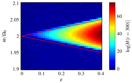
Figure 1: Numerical results showing a region of instability for a range of values of the parameters $\epsilon$ and $\omega$, for first order LF. The red lines show the predicted stability limits given in Eq. (9). The colors show the logarithm of the Hamiltonian function $H$ evaluated on the orbit after integrating the equations to $t=300$. This value should be approximately constant along the orbits, but it becomes large on orbits that spiral out to large values of $q$ and $p$. Parameters used: $\Omega_{0}=5$, $\Delta_{0}=0.05$. Initial conditions: $q=0.5$, $p=0$. The small upward shift in $\omega$ comes in at second order in $\Delta_{0}$.

In Fig. 2 we examine how, for parameters where the integration is unstable, a circle of initial conditions is stretched out into a long thin ellipse. Since the LF method is still symplectic, the area of the ellipses is preserved.

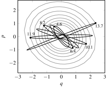
Figure 2: Numerical results illustrating that, while the first order LF method is area preserving, variable time steps can cause a parametric instability. The black ellipses are generated by taking a set of points, and propagating them forward in time using first order LF. The black dots show one of these points, which is plotted for various times (as labeled). The grey curve shows the coordinates $(q(t),p(t))$ of this point, for each of the computed time steps. Parameters: $\epsilon=0.4$, $\omega=10$, $\Omega_{0}=5$, $\Delta_{0}=0.05$.

As described above, first order LF integration of the harmonic oscillator with variable time step $\Delta(t)=\Delta_{0}(1+\epsilon\cos\omega t)$ was found to be unstable near the resonance $\omega=2\Omega_{0}$. For a nonlinear oscillator, the oscillation frequency $\Omega_{0}$ depends on the amplitude. We thus expect that the numerical integration of a nonlinear oscillator would exhibit resonant islands, rather than exhibiting global parametric instability.

For example, consider a Hamiltonian with a cubic potential

$$H(q,p)=\frac{q^{2}+p^{2}}{2}+\frac{q^{3}}{3}.$$ (18)

This Hamiltonian has an O-point at $(q,p)=(0,0)$ and an X-point at $(-1,0)$. Inside the separatrix of the X-point, this system exhibits nonlinear oscillations. For this system and first order LF, the time step variation $\Delta(t)=\Delta_{0}(1+\epsilon\cos\omega t)$ introduces an $m=1$ resonance ($\omega=\Omega_{0}$), which is readily understood by backward error analysis. Specifically, this analysis gives a term in the modified Hamiltonian which is proportional to $\sin\phi\cos\omega t$, which leads to the $m=1$ resonance.

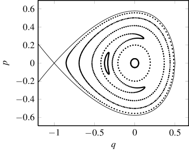
Figure 3: Surface of section plot for the cubic Hamiltonian of Eq. (18), with variable time step $\Delta(t)=\Delta_{0}(1+\epsilon\cos\omega t)$. The resonance with the time-step variation causes an $m=1$ island to open. Parameters used: $\Delta_{0}=0.3$, $\epsilon=0.6$, $\omega=0.95$. The dots are points in the surface of section (computed using CN), and the thin line is the separatrix of the X-point at $(-1,0)$.

Figure 3 shows the results of integrating this system with the CN method, and the same time steps variation. The frequency $\omega$, $0<\omega<1$, was chosen so that it would resonate with an orbit inside the separatrix. (The frequency varies with amplitude from the O-point from a maximum $\Omega=1$ at the O-point to $\Omega=0$ at the separatrix.) The dots in Fig. 3 show the Poincaré surface of section for a time–$T$ map, with $T=2\pi/\omega$. The elliptic point (O-point) of a resonant $m=1$ island is clearly seen near $(q,p)=(-0.35,0)$. We see that indeed the time dependent step size variations lead to an unphysical parametric resonance for the Hamiltonian system in Eq. (18).

3 Integration with variable time step $\Delta(q,p)$

We now turn from considering the time step variation $\Delta(t)$ to variations of the form $\Delta(q,p)$. This form of variation is perhaps more natural, since it arises when trying to optimize the time step to reduce errors in the integration method applied to an autonomous system. (We will return to this issue in Sec. 4.) In this section, we first discuss the problems that arise with this variation, and then we describe two methods by which these problems can be resolved.

Previous attempts to apply this type of time step variation to symplectic integrators have suffered from one main, although sometimes unrecognized, problem: the equations are no longer Hamiltonian. As has been pointed out[11, 12], integration of Hamiltonian’s equations

$$\frac{dz_{i}}{dt}=\epsilon_{ij}\frac{\partial H(\mathbf{z},t)}{\partial z_{j}},$$ (19)

with variable time steps satisfying $\rho(q,p)dt=d\tau$ is equivalent to changing the time variable $t$ to $\tau$, and integrating the following equations with fixed size steps in $\tau$; $\Delta\tau=h$:

$$\frac{dz_{i}}{d\tau} =\frac{1}{\rho(\mathbf{z})}\epsilon_{ij}\frac{\partial H(\mathbf{z},t)}{\partial z_{j}},$$ (20)

$$\frac{dt}{d\tau} =\frac{1}{\rho({\bf z})},$$

where $\epsilon_{12}=-\epsilon_{21}=1,\,\,\,\epsilon_{11}=\epsilon_{22}=0$ (summation assumed). Here, $\mathbf{z}=(q,p)$. As they stand, these equations are not in canonical Hamiltonian form. Because of this, the application of a symplectic integrator should not be expected to give results that are symplectic, since Eq. (20) is not a canonical Hamiltonian flow.

Once this problem has been identified, there are various approaches that can be used to find an integrator which preserves the Hamiltonian nature of Eq. (19), even with time steps given by $\rho(q,p)dt=d\tau$. In the remainder of this section, we review and discuss two methods for integrating Eqs. (20) in such a way that the symplectic nature of the original equations [Eq. (19)] is preserved. The first method is to embed these equations into a larger phase space, considering $t$ to be another coordinate. This extended phase space approach goes back to the work of Sundman [26], and has more recently been applied to numerical methods, both non-symplectic [27] and symplectic [11, 12]. In the extended phase space, the new equations can again be written in canonical Hamiltonian form, and thus integrated with any (fixed $\tau$ step) symplectic integrator. This extended phase space method is not the only way to integrate Eqs. (20) symplectically, however. A second method which we consider in this section (which only applies to one degree of freedom problems) is to recognize the the equations can be written in terms of a non-canonical bracket. Any method which preserves this bracket will then have all the nice properties of a symplectic integrator for a canonical system. We present a novel generating function approach for constructing such a method.

For the numerical results presented in this section, we will consider the Hamiltonian with a cubic potential given in Eq. (18), integrated with the two different methods. The variable time steps $\Delta=\Delta(q,p)$ are chosen so they might appear to have an $m=1$ resonance, since that is what is expected to give islands similar to the previous results of Fig. 3. Let

$$\Delta(q,p)=\Delta_{0}\left(1+a_{1}q+a_{2}p\right).$$ (21)

For the simulations reported in this paper, $a_{1}=0.5$ and $a_{2}=0.25$. For $\rho(q,p)\Delta(q,p)=h$, i.e. $\Delta t=\Delta(q,p)$ and $\Delta\tau=h$, we have

$$\rho(q,p)=\frac{h}{\Delta(q,p)}=\frac{h}{\Delta_{0}\left(1+a_{1}q+a_{2}p\right)}.$$ (22)

The step size $\Delta\tau=h$ was held fixed, and $\Delta_{0}$ was adjusted so that after a given number $N$ periods of the orbit, $t(N)$ equals $\tau(N)$. This is done so that the differences between the original and extended phase space results are due to the step size variation, rather than a change in the average step size. Integrating the original Hamilton equations (19) with fixed step size CN (i.e., with $a_{1}=a_{2}=0$) gives a result with bounded errors in energy [see Fig. 4], as is expected for symplectic integrators. However, integrating Eqs. (19) using CN with step size given by Eq. (3.2) gives errors in energy with linear growth, as also seen in Fig. 4. This lack of boundedness of the energy is to be expected, since varying the step size in this way is equivalent to integrating Eqs. (20) with fixed step size, and (20) is not a Hamiltonian system. Thus there is no reason that using a symplectic method such as CN would give results with bounded errors in energy. (Note that the Hamiltonian is just a useful diagnostic; the underlying problem is that phase space area is not conserved.)

Figure 4: CN integration of the cubic Hamiltonian [Eqs. (18) and (19)] is shown in gray, and the time transformed version of the cubic Hamiltonian [Eqs. (18) and (20), with $\rho$ as given in Eq. (3.2)] is shown in black. Parameters: $h=0.05$, $\Delta_{0}=1.05134$, $a_{1}=0.5$, $a_{2}=0.25$. Initial conditions: $(q_{0},p_{0})=(0.3,0)$.

3.1 Extended phase space method

By a well-known procedure [11, 12, 26, 27], we introduce $q_{0}=t$ and its canonically conjugate momentum $p_{0}$ and consider the Hamiltonian in extended phase space:

$$K(q,p,q_{0},p_{0})=\frac{1}{\rho(\mathbf{z})}\left(H(q,p,q_{0})+p_{0}\right),$$ (23)

again with $\mathbf{z}=(q,p)$. The canonical equations of motion are

$$\frac{dq}{d\tau} =\frac{1}{\rho(\mathbf{z})}\frac{\partial H(q,p,q_{0})}{\partial p}+\left(H+p_{0}\right)\frac{\partial}{\partial p}\left(\frac{1}{\rho}\right),$$

$$\frac{dp}{d\tau} =-\frac{1}{\rho(\mathbf{z})}\frac{\partial H(q,p,q_{0})}{\partial q}-\left(H+p_{0}\right)\frac{\partial}{\partial q}\left(\frac{1}{\rho}\right),$$ (24)

$$\frac{dq_{0}}{d\tau} =\frac{\partial K}{\partial p_{0}}=\frac{1}{\rho(\mathbf{z})},$$

$$\frac{dp_{0}}{d\tau} =-\frac{\partial K}{\partial q_{0}}=-\frac{1}{\rho(\mathbf{z})}\frac{\partial H}{\partial q_{0}}.$$

The last of these equations implies that if we choose $p_{0}(\tau=0)=-H(q(0),p(0),0)$, then ${dp_{0}}/{d\tau}=-{dH}/{d\tau}$ and $H+p_{0}$ remains zero. In this case, Eqs. (24) are identical to Eqs. (20). So, with this choice of initial condition for $p_{0}$, the actual orbit is followed and $K=0$. Note that, for this value of $p_{0}$, the other contours of $K=\rm{const.}$ are not orbits of the original system.

With the equations of motion in the form (24), we can then use a canonical symplectic integrator such as Modified LF (ML) (a semi-implicit, symmetrized version of LF; see [28, 29]) or CN with fixed time step $\Delta\tau=h$. This is the method used in Refs. [11, 12] to integrate Hamiltonian equations of motion with variable time steps for the special case $\partial H/\partial t=0$, for which $H$ and $p_{0}$ are separately constants of motion. It should be noted that in a symplectic integration of Eqs. (24), $H+p_{0}$ will be only approximately invariant, so that the results of numerically integrating Eqs. (24) will have small errors relative to the numerical results of integrating Eqs. (20).

Note that if $H$ is independent of $t$, then one needs only to integrate the equations for $q$ and $p$, since $p_{0}$ is exactly constant, and $q_{0}=t$ can be found by post-processing. So, even though this method “extends” phase space, the dimension of the system effectively remains unchanged. Therefore, there is no possibility of parametric instability if the time step is small enough.

3.2 Numerical results: extended phase space method

In this section we report numerical results using the extended phase space method [Eq. (24)] to integrate the equations from the cubic Hamiltonian [Eq. (18)], using $\rho(q,p)$ as given in Eq. (3.2). In Fig. 5 the energy errors are compared for (a) CN integration and (b) ML integration. In both cases, the black curve gives the extended phase space results, while the gray curve gives the result obtained by applying the same method with fixed step size to the original Hamiltonian equations. As for Fig. 4, the $\tau$ step $h$ was chosen to make $\tau(N)$ equal to $t(N)$ after $N$ periods of the orbit. We conclude that there is no secular change in the value of the Hamiltonian $H(q(t),p(t))$. The time step in Eq.  was chosen because it appears at first to have to potential for an $m=1$ resonance; in Sec. 4 we will describe a method to minimize the integration errors.

In Fig. 6 is shown a surface of section plot for the extended phase space CN integration. In contrast to Fig. 3, there is no resonant island caused by the time step variation. This is consistent with the comment at the end of Sec. 3.1.

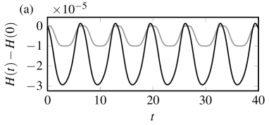
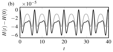
Figure 5: Extended Phase Space Method. Comparison of (a) CN and (b) ML. Shown in black is the error in energy $H(q(t),p(t))$ for the two methods. For comparison, in gray is shown the error in energy for the same method, but applied to the original uniform time step discretization of the Hamiltonian equations. Parameters: $h=0.05$, $\Delta_{0}=1.05117$, $(q_{0},p_{0})=(0.3,0)$, $a_{1}=0.5$, $a_{2}=0.25$.

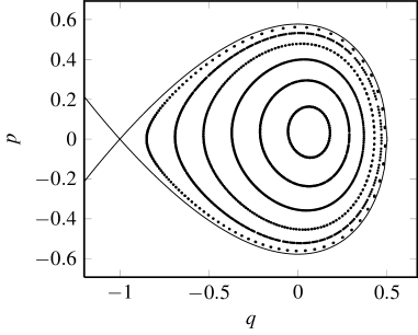
Figure 6: Surface of section plot, strobed at an arbitrary period $T$, for the extended phase space method (computed using CN). Parameters: $a_{1}=0.5$, $a_{2}=0.25$, $\Delta_{0}=0.3$. Expansion of the scale for results from longer runs show no islands anywhere inside the separatrix for any period $T$.

As a final check of the extended phase space method, a comparison was made between integrating Eqs. (20) where the step size is determined by the position in phase space as $\Delta(q,p)\propto 1/\rho(q,p)$, and integrating Eq. (19) where the step size is a function of time as determined by a reference orbit $\Delta(t)\propto 1/\rho(q_{ref}(t),p_{ref}(t))$. The reference orbit was obtained by solving the extended phase space equations [Eqs. (20)], for some initial conditions $(q_{0},p_{0})$ for which the period is $T(q_{0},p_{0})$. Time-$T$ surface of section plots for several cases give a results qualitatively similar to Fig. 3, with the time dependent step size $\Delta(t)=\Delta(q_{ref}(t),p_{ref}(t))$ giving a resonant island centered at the location of the reference orbit. This behavior is similar to the secular and unstable cases of perturbation theories discussed in A.

3.3 Non-canonical symmetrized leapfrog

In this section we discuss a second method which can be used to integrate Eqs. (20), which works for one degree of freedom systems (2D phase space). In this section, we change the notation for a point in phase space from $(q,p)$ to ${\bf z}=(x,y)$. This is done to emphasize the fact that Eqs. (20) are not in canonical Hamiltonian form.

Equations (20) are of the form $\mathbf{u}=\mathbf{m}/\rho$, where $\mathbf{u}$ is the velocity, with $\nabla\cdot\mathbf{m}=\nabla\cdot\rho\mathbf{u}=0$. The measure $\int_{V(t)}\rho dV$ is preserved over any phase space volume $V(t)$ advected with the flow. Equivalently, for the time–$t$ map $\mathbf{z}(0)\rightarrow\mathbf{z}(t)$ we have

$${\rm det}\left(\frac{\partial z_{i}(t)}{\partial z_{j}(0)}\right)=\frac{\rho(\mathbf{z}(0))}{\rho(\mathbf{z}(t))}.$$ (25)

This measure preservation suggests that a measure preserving integrator applied to this system would have the same nice properties of a symplectic integrator applied to a canonical Hamiltonian system.

The equations of motion in the form in Eq. (20) are not canonical Hamiltonian equations. However, in one degree of freedom, Eq. (20) is a Hamiltonian system in non-canonical variables and can be written in the form

$$\frac{dz_{i}}{d\tau}=[z_{i},H]_{z},\,\,\,\,\,{\rm where}\,\,\,\,\,[f,g]_{z}=\frac{1}{\rho(\mathbf{z})}\epsilon_{ij}\frac{\partial f}{\partial z_{i}}\frac{\partial g}{\partial z_{j}}$$ (26)

is a non-canonical bracket. That is, it is antisymmetric and direct calculation shows that it satisfies the Jacobi identity $[f,[g,h]_{z}]_{z}+[g,[h,f]_{z}]_{z}+[h,[f,g]_{z}]_{z}=0$.

A method of constructing a symplectic non-canonical integrator in terms of generating functions[30] starts with the condition that must hold for the time–$t$ map, which is that it must preserve the two-form

$$\rho(x,y)dx\wedge dy=\rho(X,Y)dX\wedge dY,$$ (27)

See B for more details regarding this condition. First, we define

$$\eta(x,y)=\int^{y}\rho(x,y^{\prime})dy^{\prime}$$ (28)

and

$$\xi(x,y)=\int^{x}\rho(x^{\prime},y)dx^{\prime}.$$ (29)

With these definitions, we can write

$$\rho(x,y)dx\wedge dy =dx\wedge d\eta(x,y),$$ (30)

$$\rho(X,Y)dX\wedge dY =d\xi(X,Y)\wedge dY$$ (31)

and therefore Eq. (27) becomes

$$dx\wedge d\eta(x,y)=d\xi(X,Y)\wedge dY.$$ (32)

We can consider $(X,Y)$ to be functions of $(x,y)$, and then define $p=\eta(x,y)$ and $Q=\xi(X,Y)$. These definitions, together with Eq. (32), imply that the one-form

$$\omega=pdx+QdY$$ (33)

is exact, i.e. $d\omega=0$. This in turn implies

$$\omega=dF(x,Y)=\frac{\partial F(x,Y)}{\partial x}dx+\frac{\partial F(x,Y)}{\partial Y}dY,$$ (34)

at least locally. We are led to the relations

$$\eta(x,y) =p=\frac{\partial F(x,Y)}{\partial x},$$ (35)

$$\xi(X,Y) =Q=\frac{\partial F(x,Y)}{\partial Y}.$$ (36)

Given the generating function $F(x,Y)$, we solve Eq. (35) for $Y(x,y)$ and then substitute into Eq. (36) to obtain $X(x,y)$.

In essence, what is going on is this: we are transforming to canonical variables $(x,p)$ and $(Q,Y)$, where $p=\eta(x,y)$ and $Q=\xi(X,Y)$. Then we are performing a canonical transformation $(x,p)\rightarrow(Q,Y)$ in terms of a generating function $F(x,Y)$, with $Q=\partial F/\partial Y$ and $p=\partial F/\partial x$, and expressing the results in terms of $(x,y)$, and $(X,Y)$.

The identity transformation has $X=x$ and $Y=y$ so that Eqs. (35), (36) take the form

$$\eta(x,y) =\frac{\partial F_{0}(x,y)}{\partial x},$$ (37)

$$\xi(x,y) =\frac{\partial F_{0}(x,y)}{\partial y}.$$ (38)

These relations ensure that $\partial\eta(x,y)/\partial y=\partial\xi(x,y)/\partial x=\partial^{2}F_{0}/\partial x\partial y$; by Eqs. (28), (29), these both equal $\rho(x,y)$, which is nonzero. This nondegeneracy is necessary for the inversions in Eqs. (35), (36) to work.

We now wish to construct an $O(h)$ approximation to $F(x,Y)$ in order to find a time–$h$ map ($h=\Delta\tau)$ for the system given by Eq. (20). Let us try the generating function

$$F(x,Y)=F_{0}(x,Y)+hH(x,Y).$$ (39)

From Eqs. (35) and (36) we find

$$\eta(x,y) =\frac{\partial F_{0}(x,Y)}{\partial x}-hv(x,Y),$$ (40)

$$\xi(X,Y) =\frac{\partial F_{0}(x,Y)}{\partial Y}+hu(x,Y),$$ (41)

where $u(x,y)=\partial H(x,y)/\partial y$ and $v(x,y)=-\partial H(x,y)/\partial x$. Substituting Eqs. (37) and (38) into these equations gives

$$\boxed{\eta(x,y)=\eta(x,Y)-hv(x,Y),\quad\xi(X,Y)=\xi(x,Y)+hu(x,Y).}$$ (42)

This is the form of our integrator: we integrate $\rho$ to give $\eta(x,y)$ and $\xi(x,y)$ as in Eqs. (28) and (29), iterate the first of (42) to solve for $Y$ and, after substituting for $Y$, iterate the second of (42) to solve for $X$. We do not need the explicit form for $F_{0}$ or the Hamiltonian $H$.

In order to see that Eqs. (42) are a first order accurate integrator for the system in Eq. (20), we expand to first order in $h$, and find

$$0=(Y-y)\frac{\partial\eta(x,y)}{\partial y}-hv(x,y)+O(h^{2})$$ (43)

$$(X-x)\frac{\partial\xi(x,y)}{\partial x}=hu(x,y)+O(h^{2}).$$ (44)

With Eqs. (28), (29), this leads to

$$X=x+h\frac{u(x,y)}{\rho(x,y)}+O(h^{2}),\quad Y=y+h\frac{v(x,y)}{\rho(x,y)}+O(h^{2}).$$ (45)

This implies that Eqs. (42) do constitute a first order accurate integrator for Eqs. (20). It is clear that the scheme in Eqs. (42) is the non-canonical form of the ML integrator.[29, 28] Note, however, that the system in Eqs. (42) is implicit in both $X$ and $Y$.

For the complementary generating function $G(X,y)$ we follow the same procedure, defining $\xi(x,y)$ and $\eta(x,y)$ exactly as in Eqs. (28) and (29). We can now write Eq. (27) as

$$d\xi(x,y)\wedge dy=dX\wedge d\eta(X,Y),$$ (46)

which, together with the definitions $P=\eta(X,Y)$ and $q=\xi(x,y)$, implies that

$$\omega^{\prime}=-qdy-PdX$$ (47)

is exact ($d\omega^{\prime}=0$). Therefore $\omega^{\prime}=dG(X,y)=(\partial G(X,y)/\partial X)dX+(\partial G(X,y)/\partial y)dy$ and

$$\xi(x,y)=-\frac{\partial G(X,y)}{\partial y},\quad\eta(X,Y)=-\frac{\partial G(X,y)}{\partial X}.$$ (48)

The identity is given by $G_{0}(X,y)$, where

$$\xi(x,y)=-\frac{\partial G_{0}(x,y)}{\partial y},\quad\eta(x,y)=-\frac{\partial G_{0}(x,y)}{\partial x},$$ (49)

with $-\partial^{2}G_{0}/\partial x\partial y=\rho(x,y)$. We try $G(X,y)=G_{0}(X,y)+hH(X,y),$ which leads to

$$\boxed{\xi(x,y)=\xi(X,y)-hu(X,y),\quad\eta(X,Y)=\eta(X,y)+hv(X,y).}$$ (50)

As in the case with Eqs. (42), this is the form we use as an integration scheme, and it is not necessary to obtain $G_{0}$ explicitly. Finally, a first order expansion in $h$ again gives Eqs. (45), showing that Eqs. (50) are also a first order accurate integrator for Eqs. (20).

The first order maps $(x,y)\rightarrow(X,Y)$ defined by Eqs. (42) and Eqs. (50) involve integration of a one-degree of freedom Hamiltonian system with no explicit time dependence, and thus do not exhibit a parametric instability for small enough time steps.

We have shown that both schemes in Eq. (42) and in Eq. (50) are first order accurate integrators for Eq. (20). What remains is to show that if they are applied sequentially one obtains second order accuracy. The first point is that if the maps based on $F(x,Y)$ and $G(X,y)$ are written as $T_{F}(h)$ and $T_{G}(h)$, respectively, one can show that

$$T_{F}^{-1}(h)=T_{G}(-h)$$ (51)

and of course $T_{G}^{-1}(h)=T_{F}(-h)$. This follows from inspection of Eqs. (42) and (50).

The composed map is $T(h)=T_{G}(h/2)\circ T_{F}(h/2)$ and we find

$$T(h)^{-1}=T_{F}(h/2)^{-1}\circ T_{G}(h/2)^{-1}=T_{G}(-h/2)\circ T_{F}(-h/2)=T(-h).$$ (52)

Thus, $T(h)$ is reversible and is therefore second order accurate. We call $T(h)=T_{G}(h/2)\circ T_{F}(h/2)$ non-canonical symmetrized leapfrog (NSL).

The methods outlined in this section preserve the non-canonical bracket, as does the actual time evolution of the non-canonical system. Integrators with this property are often called Poisson integrators[18, 19, 20, 21].

It is interesting to note in this context that (fixed step size) CN can be written as $T_{CN}(h)=T_{f}(h/2)\circ T_{b}(h/2)$, where $T_{f}$ is forward (explicit) Euler and $T_{b}$ is backward (implicit) Euler. Further, the implicit midpoint method $x^{\prime}=x+(h/2)u(x)+(h/2)u(x^{\prime})$ can be written as $T_{mid}(h)=T_{b}(h/2)\circ T_{f}(h/2)$. This shows that $T_{mid}=T_{f}(h/2)^{-1}\circ T_{CN}(h)\circ T_{f}(h/2)$, so that the implicit midpoint method is related to CN by a non-canonical change of variables. This implies that the implicit midpoint method is equivalent to a symplectic method under a (non-symplectic) change of variables, so it is a Poisson integrator. Therefore it can be used to integrate a canonical Hamiltonian system with all the advantages of a symplectic integrator.

3.4 Numerical results: non-canonical symmetrized leapfrog

In this section we report numerical results where the non-canonical symmetrized leapfrog (NSL) integration scheme is applied to the cubic Hamiltonian [Eq. (18)], with $\rho(x,y)=h/\Delta_{0}(1+a_{1}x+a_{2}y)$, as given in Eq. (3.2). Integrating $\rho(x,y)$ yields $\eta(x,y)=h\ln(1+a_{1}x+a_{2}y)/\Delta_{0}a_{2}$ and $\xi(x,y)=h\ln(1+a_{1}x+a_{2}y)/\Delta_{0}a_{1}$, and thus Eq. (42) with this Hamiltonian and time step variation becomes

$$\ln(1+a_{1}x+a_{2}y^{\prime}) =\ln(1+a_{1}x+a_{2}y)+\Delta_{0}a_{2}v(x),$$ (53)

$$\ln(1+a_{1}x^{\prime}+a_{2}y^{\prime}) =\ln(1+a_{1}x+a_{2}y^{\prime})+\Delta_{0}a_{1}u(y),$$

where $u=\partial H/\partial y=y$ and $v=-\partial H/\partial x=-(x+x^{2})$. The first of these can be solved for $y^{\prime}$ and then the second for $x^{\prime}$, giving a non-canonical leapfrog integrator. The second non-canonical generating function method, given in Eq. (50), can similarly be written in terms of logarithms. As described in the last section, the composition of these two methods results in a symmetrized integrator, which can be written as:

$$y^{*} =\left[(1+a_{1}x+a_{2}y)e^{\Delta_{0}a_{2}v(x)/2}-a_{1}x-1\right]/a_{2},$$ (54)

$$x^{\prime} =\left[(1+a_{1}x+a_{2}y^{*})e^{\Delta_{0}a_{1}u(y^{*})}-a_{2}y^{*}-1\right]/a_{1},$$

$$y^{\prime} =\left[(1+a_{1}x^{\prime}+a_{2}y^{*})e^{\Delta_{0}a_{2}v(x^{\prime})/2}-a_{1}x^{\prime}-1\right]/a_{2},$$

Figure 7 shows numerical results from integrating the cubic oscillator using the NSL method of Eqs. (54) (shown in black) and fixed step size symmetrized LF (shown in gray). As for the extended phase space method, we find that the NSL method with this $\rho(x,y)$ gives results with bounded errors in the energy. Again, this choice of $\rho(x,y)$ was chosen because it suggests $m=1$ resonance and leads to tractible equations; in Sec. 4.2 we show results with an optimized $\rho(x,y)$ that minimizes the time-stepping error. The surface of section for this method looks qualitatively like Fig. 6, again with no resonant islands.

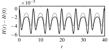
Figure 7: The NSL method applied to the cubic oscillator, with time step variations as given in Eq. (3.2). Shown in black is the error in energy. For comparison, in gray is shown the error in energy for fixed step size symmetrized LF. Parameters: $h_{0}=0.05$, $\Delta_{0}=1.0524$, $(q_{0},p_{0})=(0.3,0)$, $a_{1}=0.5$, $a_{2}=0.25$.

4 Using error estimates to find $\Delta(q,p)$

We next turn our attention to the choice of step size variation $\Delta=\Delta(q,p)$, based on an error estimator. Basing the choice of $\Delta$ on an error estimate will give step size variations which are optimized to reduce errors, in a manner to be defined.

4.1 Error estimates and minimization

As an example of an error estimate we consider CN integration of $d\mathbf{z}/dt=\mathbf{u}(\mathbf{z})$, where again $\mathbf{z}=(x,y)$. Namely, we define a map $\mathbf{z}^{\prime}=T_{h}(\mathbf{z})$ given by

$$\mathbf{z}^{\prime}=\mathbf{z}+\Delta\mathbf{u}\left((\mathbf{z}+\mathbf{z}^{\prime})/2\right),$$ (55)

where $\mathbf{z}=\mathbf{z}(t)$ and $\mathbf{z}^{\prime}=\mathbf{z}(t+\Delta)$, where $\Delta=\Delta t$ can vary as a function of $\bf z$. If $\mathbf{u}$ comes from a Hamiltonian system, CN is symplectic, but that property is not important for these considerations. We can thus let $\Delta(t)=\Delta(q_{ref}(t),p_{ref}(t))$, where $q_{ref}$ and $p_{ref}$ are the exact orbits.As mentioned in Sec. 2.1, there will be terms proportional to $d\Delta/dt$, but they will appear at the next order in $\Delta$.

The error estimate is found by expanding $\mathbf{z}(t+\Delta)$ in $\Delta$, and performing backward error analysis to obtain a local error estimate. This is a very different objective than that in the backwards error analysis in Sec. 2. In index notation we obtain

$$\frac{dz_{i}}{dt}+\frac{\Delta}{2}\frac{d^{2}z_{i}}{dt^{2}}+\frac{\Delta^{2}}{6}\frac{d^{3}z_{i}}{dt^{3}} =u_{i}\left(\mathbf{z}+\frac{\Delta}{2}\frac{d\mathbf{z}}{dt}+\frac{\Delta^{2}}{4}\frac{d^{2}\mathbf{z}}{dt^{2}}\right)$$

$$=u_{i}(\mathbf{z})+\frac{\Delta}{2}\dot{z}_{j}u_{i,j}+\frac{\Delta^{2}}{4}\ddot{z}_{j}u_{i,j}+\frac{\Delta^{2}}{8}\dot{z}_{j}\dot{z}_{k}u_{i,jk}.$$

This leads to

$$\frac{dz_{i}}{dt}=u_{i}+\Delta^{2}\left(\frac{1}{12}u_{k}u_{j,k}u_{i,j}-\frac{1}{24}u_{j}u_{k}u_{i,jk}\right),$$ (57)

which can be written in vector notation as

$$\frac{d\mathbf{z}}{dt}=\mathbf{u}+\Delta^{2}\left(\frac{1}{12}(\mathbf{u}\cdot\nabla\mathbf{u})\cdot\nabla\mathbf{u}-\frac{1}{24}\mathbf{u}\cdot(\nabla\nabla\mathbf{u})\cdot\mathbf{u}\right),$$ (58)

where ${\bf u}={\bf u}({\bf z}(t))$.

Writing the error per time step as $e=\Delta^{2}w(t)$, where $w(t)=\left|(\mathbf{u}\cdot\nabla\mathbf{u})\cdot\nabla\mathbf{u}/12-\mathbf{u}\cdot(\nabla\nabla\mathbf{u})\cdot\mathbf{u}/24\right|$, the total error in an integration is

$$E=\int_{0}^{T}edt=\int_{0}^{T}\Delta^{2}w(t)dt.$$ (59)

Now if we write the variable time step $\Delta t$ as $\Delta=(dt/d\tau)h$, where $h=\Delta\tau$ is the constant step size in $\tau$, this error takes the form

$$E=h^{2}\int d\tau\left(\frac{dt}{d\tau}\right)^{3}w(t).$$ (60)

We proceed to minimize the total error $E$ by writing $E=h^{2}\int d\tau\mathcal{L}(t,dt/d\tau)$. Ignoring the constant factor $h^{2}$, the Lagrangian $\mathcal{L}$ is given by

$$\mathcal{L}(t,dt/d\tau)=\left(dt/d\tau\right)^{3}w(t),$$ (61)

where $\tau$ is the time, and we wish to find $t(\tau)$ that minimizes $E$. This is done by forming the Euler-Lagrange equations, or equivalently by doing a Legendre transform to a Hamiltonian:

$$p=\frac{\partial\mathcal{L}}{\partial(dt/d\tau)}=3\left(\frac{dt}{d\tau}\right)^{2}w(t),$$ (62)

$$\mathcal{H}(t,p)=p\left(\frac{dt}{d\tau}\right)-\mathcal{L}(t,dt/d\tau).$$ (63)

We obtain $\mathcal{H}=2(p/3)^{3/2}w(t)^{-1/2}$. Notice that the Hamiltonian $\mathcal{H}$ is independent of the time $\tau$ and is therefore a constant of motion. Also, the Hamiltonian $\mathcal{H}$ is proportional to the Lagrangian $\mathcal{L}=(dt/d\tau)^{3}w(t)=(p/3)^{3/2}w(t)^{-1/2}$, implying that $\mathcal{L}$ is also a constant. Since $dt/d\tau=1/\rho$, we obtain an expression for the optimized time steps:

$$\rho_{opt}(\mathbf{z}(t))=Cw(t)^{1/3}.$$ (64)

This condition says that the Lagrangian, the integrand in Eq. (60), is constant with respect to $\tau$. (But the local error $e$ in Eq. (59) is not constant with respect to $t$.) A condition of this form is called an equidistribution principle[31].

4.2 Numerical results

In order to test the optimized time step, we compare numerical results using constant time step [$\Delta=\Delta_{0}$], the optimized time step

$$\Delta_{opt}=C_{opt}w(q,p)^{-1/3}\propto 1/\rho_{opt},$$ (65)

and time steps designed to give equal arc length:

$$\Delta_{arc}=C_{arc}\left[\left(\frac{\partial H}{\partial p}\right)^{2}+\left(\frac{\partial H}{\partial q}\right)^{2}\right]^{-1/2}.$$ (66)

With $\Delta_{arc}$, the magnitude of the phase space velocity $\vec{v}\equiv(\partial q/\partial\tau,\partial p/\partial\tau)$ is constant. Numerical results for these three choices of $\Delta$ are shown in Fig. 8, using the CN integrator in extended phase space. For each of these methods, fixed steps in $\tau$ of size $\Delta\tau=h$ were used. The constant of proportionality $C$ in $\Delta=C/\rho$ was then chosen so that, after $N$ periods of the orbit, $\tau(N)$ equals $t(N)$. This is done in order to distinguish the effect of varying the step size as a function of $(q,p)$ from the effect of reducing the overall average step size.

Two diagnostics of the numerical integrations related to the local error are shown in Fig. 8, for $\Delta=\Delta_{0}$ (light gray), $\Delta_{arc}$ (dark gray), and $\Delta_{opt}$ (black). They are the local error $\Delta^{2}w(t)$ as a function of time and $\Delta^{3}w(\tau)$, proportional to the integrand in Eq. (60), as a function of $\tau$, respectively. Variations in step size given by $\Delta_{arc}$ reduce the error compared to the fixed step size integration, at almost all points along the orbit. Variations given by $\Delta_{opt}$ further reduce the local error in some places, while allowing the local error to increase in others. As seen in Fig. 8b, this variation has the effect of spreading the local error along the orbit, so that $\Delta^{3}w(t)$ is constant as a function of $\tau$, as required by the equidistribution principle.

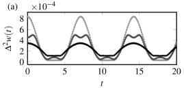
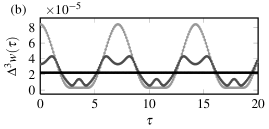
Figure 8: Comparison of the errors for the extended phase space CN method, for three time-step variations, $\Delta=\rm{const.}$ (light gray), $\Delta_{arc}$ (dark gray), and $\Delta_{opt}$ (black). (a) The local error as a function of time $t$ [integrand of Eq. (59)], and (b) the local error as a function of $\tau$ [$h^{3}$ times the integrand of Eq. (60)]. Parameters: $h=0.1$, $(q_{0},p_{0})=(0.4,0)$, $\Delta_{0}=0.1$, $C_{arc}=0.41$, $C_{opt}=0.28$

As a further test to check if $\Delta_{opt}$ really minimizes $E$ [as defined in Eq. (60)], we also show numerical results where $E$ is computed for

$$\Delta_{\beta} = C_{\beta}\left[(1-\beta)+\beta w(q,p)^{-1/3}\right],$$ (67)

$$\propto \left[(1-\beta)\Delta_{0}+\beta\Delta_{opt}\right],$$ (68)

where $C_{\beta}$ is chosen as above for each $\beta$, for a range of $\beta$. When $\beta=0$, the time steps are uniform, and when $\beta=1$ the time steps are given by $\Delta_{opt}$. The results are shown in Fig. 9. As seen in the inset in Fig. 9, the error is indeed a minimum for $\beta=1$, with $E=2.22\times 10^{-4}$. For comparison, using $\Delta=\Delta_{arc}$ gives $E=2.48\times 10^{-4}$, and $\Delta=\Delta_{0}={\rm const.}$ gives $E=3.29\times 10^{-4}$

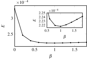
Figure 9: The global error [Eq. (60)], over the time $T=20$, for the time step variation $\Delta_{\beta}$ [Eq. (67)]. As seen in the inset, the error is minimized with $E=2.22\times 10^{-4}$ for $\beta=1$, for which $\Delta_{\beta}=\Delta_{opt}$. For comparison, using $\Delta=\Delta_{arc}$ gives $E=2.48\times 10^{-4}$, and $\Delta=\Delta_{0}$ gives $E=3.29\times 10^{-4}$.

5 Summary

In this paper we have studied variable and adaptive time stepping for symplectic integrators, of importance for particle-in-cell codes, for accelerators, for tracing magnetic field lines, and for ray tracing. We have shown that problems observed in the literature for symplectic integrators with variable time steps fall into two categories. In the first, with time step $\Delta=\Delta(t)$, the integrators are still symplectic but results can exhibit parametric instabilities associated with resonances between the time step variation and the orbital motion. We have characterized these instabilities by means of backward error analysis and numerical integrations. In the second category, the time steps depend on position in phase space, $\Delta=\Delta(q,p)$, and integrators which are symplectic for $\Delta={\rm const.}$ are no longer symplectic.

We have discussed symplectic integrators for $\Delta=\Delta(q,p)$ of two basic varieties. In both, we start by modifying the time variable $t\rightarrow\tau$ such that $\rho(q,p)dt=d\tau$ and $\rho(q,p)\propto\Delta(q,p)^{-1}$ and we do uniform time stepping in $\tau$. In the first method, one extends the phase space $(q_{1},...,q_{n},p_{1},...,p_{n})\longrightarrow(q_{0},q_{1},...,q_{n},p_{0},p_{1},...,p_{n})$, with $q_{0}=t$ and $p_{0}$ its canonical conjugate. In this extended phase space with $\tau$ taking the place of time and $\Delta\tau={\rm const.}$, any numerical integrator can be used and we investigate modified leapfrog[28, 29], symmetrized to be of second order, and Crank-Nicolson. In the second variety of integrator, we start by noticing that the equations to be solved, written as functions of $\tau$, are in Hamiltonian form with non-canonical variables for one degree of freedom problems. We then construct a Poisson integrator (the analog of a symplectic integrator but for non-canonical variables) in terms of a generating function of mixed variables, which is a generalization of the mixed variable generating functions for canonical variables[32]. We also show how to symmetrize this integrator to obtain second order accuracy, obtaining the non-canonical symmetrized leapfrog integrator.

We have investigated these integrators for a model Hamiltonian system (the cubic oscillator) and found no parametric instabilities or growth or decay due to lack of phase space conservation.

We have also investigated adaptive time-stepping, focusing on minimizing the norm of the error obtained by backward error analysis. We have applied this optimal time-stepping to the model Hamiltonian system and found that indeed the error is minimized while the advantages of symplectic integration are preserved.

Appendix A Variable time steps and perturbation theory

Two main time step variations are considered in the literature: $\Delta=\Delta(t)$ and $\Delta=\Delta(q,p)$. The phase space dependent variation $\Delta(q,p)$ is natural because the errors in an integration method of an autonomous system depend only on phase space position. Indeed, we found that error analysis (as in Sec. 4) for the integration method gives errors which depend on location in phase space $(q,p)$.

The second kind of variation $\Delta(t)$ comes from a type of perturbation analysis. The logic is as follows: orbits $(q(t),p(t))$ of a Hamiltonian system are often periodic, and because of this, time step variations $\Delta(q,p)$ on the orbit should also be periodic. That is, we can substitute $q(t)$ and $p(t)$ to arrive at $\Delta(t)\equiv\Delta(q(t),p(t))$, giving periodic time dependence.

This argument ignores the stability issue: if an orbit is perturbed, the period of $\Delta(q(t),p(t))$ will vary, but this will not occur for a prescribed $\Delta(t)$.

It has been observed[5, 7, 8, 9] that such a $\Delta(t)$ is not a stable method for varying the time step of a symplectic integrator. Some analysis (see Ref. [16] and Sec. 2) shows that this does not work because it introduces parametric resonances into the system. As we have shown in Sec. 2, the integrator is still symplectic in this case, but the problem is that the modified equations (in the case of a harmonic oscillator) take the form of the Mathieu equation, which is still Hamiltonian but can be unstable.

We here review how such parametric instabilities and secularities arise in perturbation theory, to help us understand the parametric instabilities of Sec. 2.1.

Secularities show up in perturbation theories in the following manner. Take the system

$$\ddot{x}+x+\epsilon x^{3}=0.$$ (69)

A straightforward perturbation method involves iterating

$$\ddot{x}_{k+1}+x_{k+1}=-\epsilon x_{k}^{3}.$$ (70)

For $x_{0}=b\cos t$, we obtain

$$\ddot{x}_{1}+x_{1}=-\epsilon b^{3}\left(\frac{1}{4}\cos 3t+\frac{3}{4}\cos t\right).$$ (71)

The last term on the right is resonant and leads to a secularity,

$$x_{1}=b\cos t-\frac{3\epsilon b^{3}}{8}t\sin t+\cdots$$ (72)

However, it is clear from Eq. (69) that the exact solution is bounded: the energy is $H=\dot{x}^{2}/2+x^{2}/2+\epsilon x^{4}/4$. The $t\sin t$ term represents the frequency shift that occurs in Eq. (69) because of the term proportional to $\epsilon$, and is accurate for short time, but clearly wrong for long time.

For an example of a perturbation approach with a parametric instability, we consider instead

$$\ddot{x}+x+\epsilon x^{2}=0,$$ (73)

with the perturbation method

$$\ddot{x}_{k+1}+x_{k+1}=-\epsilon x_{k}x_{k+1}.$$ (74)

(We choose a different model in order to obtain again results at first order in the perturbation theory.) From $x_{0}=b\cos t$ we obtain

$$\ddot{x}_{1}+\left(1+\epsilon b\cos t\right)x_{1}=0.$$ (75)

Using $\tau=t/2$, this is the Mathieu equation $d^{2}x_{1}/d\tau^{2}+\left(a+2q\cos 2\tau\right)x_{1}=0$, with $a=4$ and $q=2\epsilon b$, for which a parametric instability occurs. As in the secular example above, the exponential growth represents the correct frequency shift for small time, but is wrong for longer time. Indeed, the energy is $H=\dot{x}^{2}/2+x^{2}/2+\epsilon x^{3}/3$, and for initial conditions near $x=\dot{x}=0$ the solution cannot grow indefinitely. As we have seen in Sec. 2.1, parametric instabilities for $\Delta t=\Delta(t)$ have a very similar character.

Appendix B Non-canonical brackets and forms

In this appendix we first describe the conditions that change of variables must satisfy so that the form of a set of equations defined with a non-canonical bracket is preserved. We then show that the flow of a Hamiltonian system written in non-canonical variables, such as Eq. (20) (one degree of freedom), generates a change of variables satisfying these conditions.

First define the non-canonical bracket

$$[f({\bf z}),g({\bf z})]_{z}\doteq\frac{1}{\rho({\bf z})}\epsilon_{ij}\frac{\partial f({\bf z})}{\partial z_{i}}\frac{\partial g({\bf z})}{\partial z_{j}}.$$ (76)

In one degree of freedom, $[\cdot,\cdot]_{z}$ is indeed a non-canonical bracket, which can be verified by proving the Jacobi identity. In more that one degree of freedom, this does not define a legitimate non-canonical bracket, since it does not satisfy the Jacobi identity.

We now ask what change of variables $\mathbf{Z}=\mathbf{Z}(\mathbf{z})$ preserves the form, i.e., what conditions must this change of variables satisfy so that

$$[f({\bf z}),g({\bf z})]_{z}=[f({\bf Z}),g({\bf Z})]_{Z},$$ (77)

where

$$[f({\bf Z}),g({\bf Z})]_{Z}\doteq\frac{1}{\rho({\bf Z})}\epsilon_{mn}\frac{\partial f({\bf Z})}{\partial Z_{m}}\frac{\partial g({\bf Z})}{\partial Z_{n}}.$$ (78)

Using the definitions of these brackets and the chain rule, Eq. (77) becomes

$$\frac{1}{\rho({\bf z})}\epsilon_{ij}\frac{\partial Z_{m}}{\partial z_{i}}\frac{\partial f({\bf z})}{\partial Z_{m}}\frac{\partial Z_{n}}{\partial z_{j}}\frac{\partial g({\bf z})}{\partial Z_{n}}=\frac{1}{\rho({\bf Z})}\epsilon_{mn}\frac{\partial f({\bf Z})}{\partial Z_{m}}\frac{\partial g({\bf Z})}{\partial Z_{n}}.$$ (79)

In order for this to be true, we require that

$$\frac{1}{\rho({\bf z})}\epsilon_{ij}\frac{\partial Z_{m}}{\partial z_{i}}\frac{\partial Z_{n}}{\partial z_{j}}=\frac{1}{\rho({\bf Z})}\epsilon_{mn},$$ (80)

or, written in matrix form, that

$$MEM^{T}=\frac{\rho(\mathbf{z})}{\rho(\mathbf{Z})}E,\,\,\,\,{\rm where}\,\,\,\,M_{ij}=\frac{\partial Z_{i}}{\partial z_{j}},\,\,\,\,\,\,\,E_{ij}=\epsilon_{ij}.$$ (81)

If this condition is satisfied, then the transformation ${\bf z}\to{\bf Z}$ preserves this specific non-canonical symplectic structure.

The next issue is to show that the time evolution operator for Eq. (20) generates a map with this property. Since Eq. (20) can be written in terms of the non-canonical bracket as

$$\frac{dz_{i}}{d\tau}=[z_{i},H]_{z},$$ (82)

then, for infinitesimal $h$, if we define $z_{i}=z_{i}(0)$ and $Z_{i}=z_{i}(h)$ we have

$$Z_{i}=z_{i}+h[z_{i},H]_{z}.$$ (83)

Taking the bracket of $Z_{i}$ and $Z_{j}$ therefore gives

$$[Z_{i},Z_{j}]_{z} =[z_{i},z_{j}]_{z}+h[[z_{i},H]_{z},z_{j}]_{z}+h[z_{i},[z_{j},H]_{z}]_{z}$$ (84)

$$=[z_{i},z_{j}]_{z}+h[[z_{i},H]_{z},z_{j}]_{z}+h[[H,z_{j}]_{z},z_{i}]_{z}$$ (85)

$$=[z_{i},z_{j}]_{z}+h[[z_{i},z_{j}]_{z},H]_{z}.$$ (86)

The last equality follows from the Jacobi identity. This equals

$$[Z_{i},Z_{j}]_{z} =\epsilon_{ij}\left(\frac{1}{\rho(\mathbf{z})}+h[{1}/{\rho},H]_{z}\right)$$ (87)

$$=\epsilon_{ij}\left(\frac{1}{\rho(\mathbf{z})}+(Z_{k}-z_{k})\frac{\partial}{\partial z_{k}}\left(\frac{1}{\rho(\mathbf{z})}\right)\right)$$ (88)

$$=\frac{\epsilon_{ij}}{\rho(\mathbf{Z})}=[Z_{i},Z_{j}]_{Z}.$$ (89)

Thus, the time evolution operator for an infinitesimal time step $h$ preserves the non-canonical symplectic structure. This fact is the basis for finding a non-canonical generating function in Sec. 3.3 that gives a first order accurate integrator for the non-canonical Hamiltonian system.

Finally, we express these ideas in terms of differential forms. Eq. (80) can be written

$$\rho(\mathbf{Z})\frac{\partial Z_{k}}{\partial z_{i}}\epsilon_{kl}\frac{\partial Z_{l}}{\partial z_{j}}=\rho(\mathbf{z})\epsilon_{ij}.$$ (90)

From this, we obtain the expression

$$\rho(\mathbf{Z})(\partial Z_{k}/\partial z_{i})\epsilon_{kl}(\partial Z_{l}/\partial z_{j})dz_{i}dz_{j}=\rho(\mathbf{z})\epsilon_{ij}dz_{i}dz_{j},$$ (91)

or

$$\rho(\mathbf{Z})\epsilon_{kl}dZ_{k}dZ_{l}=\rho(\mathbf{z})\epsilon_{ij}dz_{i}dz_{j}.$$ (92)

Since we are considering only 2D phase space, this can be expressed as

$$\rho(X,Y)dX\wedge dY=\rho(x,y)dx\wedge dy.$$ (93)

Eq. (93) is the two-form used in Sec. 3.3.

References

References

- [1] P J Channell and C Scovel. Symplectic integration of Hamiltonian systems. Nonlinearity, 3(2):231, 1990.
- [2] B. J. Leimkuhler, S. Reich, and R. D. Skeel. Integration methods for molecular dynamics. In J. P. Mesirov, K. Schulten, and D. Sumners, editors, Mathematical Approaches to Biomolecular Structure and Dynamics, volume 82 of IMA Volumes Math. Appl., page 161. Springer, 1996.
- [3] Joseph A. Morrone, Ruhong Zhou, and B. J. Berne. Molecular dynamics with multiple time scales: How to avoid pitfalls. J. Chem. Theory Comput., 6(6):1798–1804, 2010.
- [4] Robert D. Skeel and C.W. Gear. Does variable step size ruin a symplectic integrator? Physica D: Nonlinear Phenomena, 60(1-4):311–313, 1992.
- [5] Robert D. Skeel. Variable step size destabilizes the Störmer/leapfrog/Verlet method. BIT Numerical Mathematics, 33(1):172–175, 1993.
- [6] M. P. Calvo and J. M. Sanz-Serna. The development of variable-step symplectic integrators, with application to the two-body problem. SIAM J. Sci. Comput., 14(4):936–952, July 1993.
- [7] M.H. Lee, M.J. Duncan, and H.F. Levison. Variable timestep integrators for long-term orbital integrations. In D. A. Clarke and M. J. West, editors, Computational Astrophysics, volume 32 of Proc. 12th Kingston Meeting, San Franscisco, 1997. Astronmical Society of the Pacific.
- [8] Joseph P. Wright. Numerical instability due to varying time steps in explicit wave propagation and mechanics calculations. Journal of Computational Physics, 140(2):421 – 431, 1998.
- [9] Robert D. Skeel. Comments on “Numerical instability due to varying time steps in explicit wave propagation and mechanics calculations” by Joseph P. Wright. Journal of Computational Physics, 145(2):758 – 759, 1998.
- [10] Brett Gladman, Martin Duncan, and Jeff Candy. Symplectic integrators for long-term integrations in celestial mechanics. Celestial Mechanics and Dynamical Astronomy, 52(3):221–240, 1991.
- [11] E. Hairer. Variable time step integration with symplectic methods. Applied Numerical Mathematics, 25(2-3):219 – 227, 1997. Special Issue on Time Integration.
- [12] S. Reich. Backward error analysis for numerical integrators. SIAM J. on Numerical Analysis, 36(5):1549–1570, 1999.
- [13] P. Hut, J. Makino, and S. McMillan. Building a better leapfrog. The Astrophysical Journal, 443:L93–L96, April 1995.
- [14] C. W. Hirt. Heuristic stability theory for finite-difference equations. Journal of Computational Physics, 2(4):339 – 355, 1968.
- [15] Steven P. Auerbach and Alex Friedman. Long-time behaviour of numerically computed orbits: Small and intermediate timestep analysis of one-dimensional systems. Journal of Computational Physics, 93(1):189–223, 1991.
- [16] Robert Piché. On the parametric instability caused by step size variation in Runge-Kutta-Nyström methods. Mathematics Report 73, Tampere University of Technology, 1998.
- [17] P.J. Morrison. Hamiltonian fluid dynamics (and references therein). In Jean-Pierre Françoise, Gregory L. Naber, and Tsou Sheung Tsun, editors, Encyclopedia of Mathematical Physics, pages 593 – 600. Academic Press, Oxford, 2006.
- [18] Ge Zhong and Jerrold E. Marsden. Lie-Poisson Hamilton-Jacobi theory and Lie-Poisson integrators. Physics Letters A, 133(3):134 – 139, 1988.
- [19] Ge Zhong. Generating functions, Hamilton-Jacobi equations and symplectic groupoids on Poisson manifolds. Indiana University Mathematics Journal, 39(3):18, 1990.
- [20] P.J. Channell and J.C. Scovel. Integrators for Lie-Poisson dynamical systems. Physica D: Nonlinear Phenomena, 50(1):80 – 88, 1991.
- [21] B. Karasözen. Poisson integrators. Mathematical and Computer Modelling, 40(11-12):1225 – 1244, 2004.
- [22] Haruo Yoshida. Construction of higher order symplectic integrators. Physics Letters A, 150(5-7):262 – 268, 1990.
- [23] MP Calvo, A. Murua, and JM Sanz-Serna. Modified equations for ODEs. In Chaotic numerics: an International Workshop on the Approximation and Computation of Complicated Dynamical Behavior, Deakin University, Geelong, Australia, July 12-16, 1993, volume 172 of Contemp. Math., pages 63–74. Amer Mathematical Society, 1994.
- [24] Giancarlo Benettin and Antonio Giorgilli. On the Hamiltonian interpolation of near-to-the identity symplectic mappings with application to symplectic integration algorithms. Journal of Statistical Physics, 74:1117–1143, 1994.
- [25] E. Hairer. Backward analysis of numerical integrators and symplectic methods. Ann. Numer. Math., 1(1-4):107–132, 1994.
- [26] K. F. Sundman. Mémoire sur le problème dès trois corps. Acta Math., 36:105–179, 1912.
- [27] K. Zare and V. Szebehely. Time transformations in the extended phase-space. Celestial Mechanics and Dynamical Astronomy, 11:469–482, 1975.
- [28] John M. Finn and Luis Chacón. Volume preserving integrators for solenoidal fields on a grid. Physics of Plasmas, 12(5):054503, 2005.
- [29] C. A. Fichtl, J. M. Finn, and K. L. Cartwright. An arbitrary curvilinear coordinated method for particle-in-cell modeling. submitted to JCP, 2011.
- [30] A. L. Islas, D. A. Karpeev, and C. M. Schober. Geometric integrators for the nonlinear Schrödinger equation. Journal of Computational Physics, 173(1):116 – 148, 2001.
- [31] V D Liseikin. Grid Generation Methods. Springer, Berlin, 1999.
- [32] Herbert Goldstein, Charles P Poole, and John L. Safko. Classical Mechanics. Addison Wesley, 3rd edition, 2002.