Asymptotics of orthogonal polynomials with complex varying quartic weight: global structure, critical point behaviour and the first Painlevé  equation

M. Bertola^†‡, A. Tovbis^♯

^† Centre de recherches mathématiques, Université de Montréal
C. P. 6128, succ. centre ville, Montréal, Québec, Canada H3C 3J7
^‡ Department of Mathematics and Statistics, Concordia University
1455 de Maisonneuve W., Montréal, Québec, Canada H3G 1M8
^♯ University of Central Florida Department of Mathematics
4000 Central Florida Blvd. P.O. Box 161364 Orlando, FL 32816-1364

Abstract

We study the asymptotics of recurrence coefficients for monic orthogonal polynomials $\pi_{n}(z)$ with the quartic exponential weight $\exp\left[-N\left(\frac{1}{2}z^{2}+\frac{1}{4}tz^{4}\right)\right]$, where $t\in{\mathbb{C}}$ and $N\in{\mathbb{N}}$, $N\rightarrow\infty$. Our goals are: A) to describe the regions of different asymptotic behaviour (different genera) globally in $t\in{\mathbb{C}}$; B) to identify all the critical points, and; C) to study in details the asymptotics in a full neighborhood near of critical points (double scaling limit), including at and near the poles of Painlevé I solutions $y(v)$ that are known to provide the leading correction term in this limit. Our results are: A) We found global in $t\in{\mathbb{C}}$ asymptotic of recurrence coefficients and of “square-norms” for the orthogonal polynomials $\pi_{n}$ for different configurations of the contours of integration. Special code was developed to analyze all possible cases. B) In addition to the known critical point $t_{0}=-\frac{1}{12}$, we found new critical points $t_{1}=\frac{1}{15}$ and $t_{2}=\frac{1}{4}$. C) We derived the leading order behavior of the recurrence coefficients (together with the error estimates) at and around the poles of $y(v)$ near the critical points $t_{0},t_{1}$ in what we called the triple scaling limit. We proved that the recurrence coefficients have unbounded $\mathcal{O}(N^{-1})$-size (in $t$) “spikes” near the poles of $y(v)$ and calculated the “universal” shape of these spikes for different cases (depending on the critical point $t_{0,1}$ and on the configuration of the contours of integration). The nonlinear steepest descent method for Riemann-Hilbert Problem (RHP) is the main technique used in the paper. We note that the RHP near the critical points is very similar to the RHP describing the semiclassical limit of the focusing NLS near the point of gradient catastrophe that the authors solved in [5]. Our approach is based on the technique developed in [5].

1 Introduction and main results

In this paper we consider monic polynomials $\pi_{n}(z)$, orthogonal with respect to the quartic exponential weight $e^{-Nf(z,t)}$, where $f(z,t)=\frac{1}{2}z^{2}+\frac{1}{4}tz^{4}$, $t\in{\mathbb{C}}$ and $N\in{\mathbb{N}}$. As $z\rightarrow\infty$, the weight function is exponentially decaying in four sectors $S_{j}$ of the opening $\pi/4$, centered around the rays $\Omega_{j}=\{z:~{}\arg z=-\frac{\arg t}{4}+\frac{\pi(j-1)}{2}\}$, $j=1,2,3,4$. We consider the most general case when the polynomials $\pi_{n}(z)$ are integrated on the “cross” formed by the rays $\Omega_{j}$, where the rays $\Omega_{1,2}$ are oriented outwards (away from the origin) and the rays $\Omega_{3,4}$ - inwards. The corresponding bilinear form is

$$\langle p,q\rangle_{\varrho_{1},\varrho_{2},\varrho_{3},\varrho_{4}}=\sum_{j=1}^{4}\varrho_{j}\int_{\Omega_{j}}p(z)q(z)e^{-Nf(z,t)}dz,\ \ \ f(z,t):=\frac{1}{2}z^{2}+\frac{1}{4}tz^{4}$$ (1-1)

where $\varrho_{j}$ are fixed complex numbers chosen to satisfy $\varrho_{1}+\varrho_{2}=\varrho_{3}+\varrho_{4}$. Moreover, since multiplying all the $\varrho_{j}$’s by a common nonzero constant does not affect the families orthogonal polynomials, these parameters are only defined modulo the action of the group ${\mathbb{C}}^{*}$ and hence the orthogonal polynomials are naturally parametrized by points in ${\mathbb{C}}\mathbb{P}^{2}$.

Figure 1: The contours of integration and the asymptotic directions. The contour $\varpi_{4}$ is homologically equal to $-\varpi_{1}-\varpi_{2}-\varpi_{3}$, and it is unnecessary for the definition of the pairing (1-2).

Alternatively, the bilinear form (1-1) can be represented as

$$\langle p,q\rangle_{\vec{\nu}}=\sum_{k=1}^{3}\nu_{k}\int_{\varpi_{k}}p(z)q(z)e^{-Nf(z,t)}dz,$$ (1-2)

$$\nu_{1}=-\varrho_{1}\ ,\qquad\nu_{2}=-\varrho_{2}-\varrho_{1}\ ,\qquad\nu_{3}=-\varrho_{4}$$ (1-3)

where $\varpi_{j}$, $j=1,2,3$, are simple contours emanating from $\infty$ along $\Omega_{j}$ and returning to $\infty$ along $\Omega_{j+1}$ [3] (Fig. 1).

Then in the case a) we have $\nu_{2}\neq 0$ (and we therefore can, and will, normalize it to be $\nu_{2}=1$) and the following three cases are possible:

1. The ”generic case”: $\nu_{1}\nu_{3}\neq 0$, $\nu_{1}\neq 1\neq\nu_{3}$, so that there are three contours $\varpi_{j}$ in (1-2);

2. The ”consecutive wedges”: either $\nu_{1}$ or $\nu_{3}$ (but not both) is zero so that there are two adjacent contours $\varpi_{j}$ in (1-2);

3. The ”real axis”: $\nu_{3}=0$ and $\nu_{1}=1$.

The remaining case b): $\varrho_{1}+\varrho_{2}=0$, corresponds to $\nu_{2}=0$, so that the following three cases are possible:

1. The ”single wedge”: $\nu_{1}=0$, so that there is only one contour $\varpi_{3}$ in (1-2), for which we can, and will, set $\nu_{3}=1$;

2. The ”opposite wedges, generic”: $\nu_{1}\nu_{3}\neq 0$ and $\nu_{1}\neq\nu_{3}$;

3. The ”opposite wedges, symmetric”: $\nu_{1}=\nu_{3}\neq 0$.

The orthogonality condition for the monic polynomials $\pi_{n}(z)$ can now be written as

$$\langle\pi_{n},z^{k}\rangle_{\vec{\nu}}={\mathbf{h}}_{n}\delta_{nk},~{}~{}~{}~{}~{}~{}~{}k=0,1,2,\cdots,n,~{}~{}~{}~{}\vec{\nu}=(\nu_{1},\nu_{2},\nu_{3}),$$ (1-4)

where the coefficient ${\mathbf{h}}_{n}$ can also be written as ${\mathbf{h}}_{n}=\langle\pi_{n},\pi_{n}\rangle_{\vec{\nu}}$ and hence is the equivalent of the “square norm” of $\pi_{n}$ (but it is in general a complex number). The existence of orthogonal polynomials $\pi_{n}(z)$ is not a priori clear. However, if three consecutive monic polynomials exists, they are related by a three-term recurrence relation

$$\pi_{n+1}=(z-\beta_{n})\pi_{n}(z)-\alpha_{n}\pi_{n-1}(z),$$ (1-5)

where $\alpha_{n}=\alpha_{n}(t,N)$, $\beta_{n}=\beta_{n}(t,N)$ are called recurrence coefficients.

If the bilinear pairing is invariant under the map $z\mapsto-z$ then it follows immediately that the orthogonal polynomials are even or odd according to their degree and thus $\beta_{n}=0\,,\forall n\in{\mathbb{N}}$ (for example in case (a1) with coefficients $\nu_{1}=\nu_{3}$, and $\nu_{2}=0$). Then the remaining recurrence coefficients $\alpha_{n}$ satisfy

$$\alpha_{n}[1+t(\alpha_{n+1}+\alpha_{n}+\alpha_{n-1})]=\frac{n}{N},$$ (1-6)

which is known in literature as the string equation or the Freud equation [15]. We are interested in the asymptotic limit of $\alpha_{n},\beta_{n}$ as $N\rightarrow\infty$ and $\frac{n}{N}=x>0$ is fixed and finite, so we will use notations $\alpha_{n}=\alpha_{n}(x,t),~{}\beta_{n}=\beta_{n}(x,t)$ instead of $\alpha_{n}=\alpha_{n}(t,N)$, $\beta_{n}=\beta_{n}(t,N)$.

In the case of $\nu_{2}=-1$ and $x=1$ (that is, $n=N$) and a fixed $t\in(-\frac{1}{12},0)$, the asymptotics of $\alpha_{n},~{}\beta_{n}$ was obtained in [10] as

$$\alpha_{n}(1,t)=\frac{\sqrt{1+12t}-1}{6t}+O(n^{-1}),$$ (1-7)

and $\beta_{n}$ decaying exponentially as $n\rightarrow\infty$. (To be more precise, Theorem 1.1 from [10] states that there exists some $n_{0}=n_{0}(t)$, such that $\alpha_{n}(1,t),\beta_{n}(1,t)$ exists for all $n\geq n_{0}$ and have the above mentioned asymptotics.) In the non symmetrical case, however, the recurrence coefficients $\beta_{n}$ are, generically, different from zero. Then, instead of (1-6), we have the general Freud system (we indicate how to derive it in Section. 3.1):

$$0 {\hskip-20.0pt}=\beta_{n}+t\left[(2\beta_{n}+\beta_{n+1})\alpha_{n+1}+(\beta_{n}^{2}+2\alpha_{n}(1-\delta_{n0}))\beta_{n}+\alpha_{n}\beta_{n-1}(1-\delta_{n0})\right],$$ (1-8)

$$\frac{n}{N} {\hskip-20.0pt}=\alpha_{n}+t\left[\alpha_{n}\alpha_{n-1}+\alpha_{n}^{2}(1-\delta_{n0})+\alpha_{n+1}\alpha_{n}+\beta_{n}^{2}\alpha_{n}+\alpha_{n}\beta_{n-1}(\beta_{n}+\beta_{n-1})\right].$$ (1-9)

where $\delta_{ij}$ denotes the Kronecker’s delta. Assuming that $\beta_{n}\to\beta$ and $\alpha_{n}\to\alpha$ as $n\rightarrow\infty$, we obtain two leading order algebraic equations

$$\beta(1+6t\alpha+t\beta^{2})=0\ ,\qquad\alpha\left(1+3t\alpha+3t\beta^{2}\right)=x,$$ (1-10)

which have two solutions

$$\beta=0,\qquad~{}~{}~{}~{}~{}~{}~{}~{}~{}~{}~{}~{}\alpha=\frac{\sqrt{1+12xt}-1}{6t},$$ (1-11)

$$\rm{~{}and}$$ (1-12)

$$\beta^{2}=-6\alpha-\frac{1}{t}\ ,\qquad\alpha=\frac{\sqrt{1-15xt}-1}{15t}.$$ (1-13)

The dependence on $x$ is rather fictitious: indeed, looking at the pairing (1-1) one sees that if $0<x\neq 1$ then we can rescale $\widetilde{z}=\frac{z}{\sqrt{x}}$, $\widetilde{t}=x\,t$ and obtain the case $N=n$ ($x=1$) without loss of any generality; we shall assume this done throughout the paper, but still distinguish $n$ and $N$ because they play a slightly different role.

We point out that the asymptotics of the recurrence coefficients for orthogonal polynomials with integration on the real axis (and analytic continuation thereof in the complex $t$–plane) satisfies identically $\beta_{n}=0$, and hence only the first solution (1-11) is relevant. However, in view of applications to combinatorics of maps, it is not clear what role, if any, the second solution (1-13) play. It could be, perhaps, of some relevance that the critical point $t_{1}=\frac{1}{15}$ of the second solution is actually closer to the origin than the critical point $t_{0}=-\frac{1}{12}$ of the “standard” (first) solution.

The recurrence coefficients problem was studied in [10], following earlier work [14], for negative values of $t\in(-\frac{1}{12},0)$. For definiteness we shall assign $\arg(t)=\pi$, so that (refer to Fig. 1) the contour $\varpi_{1}$ consists of the two rays $\arg(z)=\pm\frac{\pi}{4}$, $\varpi_{2}$ of $\arg(z)=\frac{\pi}{4},\frac{3\pi}{4}$ and $\varpi_{3}$ of $\arg(z)=\frac{3\pi}{4},\frac{5\pi}{4}$ (other determinations of $\arg(t^{\frac{1}{4}})$ would only reshuffle the contours around). To describe the results of [10] and to set the stage for our results, we need to recall that the general solution of the Painlevé I (P1) equation

$$y^{\prime\prime}(v)=6y^{2}(v)-v\$$ (1-14)

is parametrized by two parameters in terms of a certain Riemann–Hilbert problem described in Section 2. It is known that any solution to P1 has infinitely many poles with a Laurent expansion of the form

$$y(v)=\frac{1}{(v-v_{p})^{2}}+\frac{v_{p}}{10}(v-v_{p})^{2}+\frac{1}{6}(v-v_{p})^{3}+\beta(v-v_{p})^{4}+\frac{v_{p}^{2}}{300}(v-v_{p})^{6}+\mathcal{O}((v-v_{p})^{7}).$$ (1-15)

The Painlevé property asserts that the only singularities that can occur are of this form, that is, the position of these poles depends on the chosen solution, and it is largely unknown, except for some asymptotic localization of the remote poles, see, for example, [16]. In the following theorem and henceforth we use notations $\alpha_{n}(t)=\alpha_{n}(1,t),~{}\beta_{n}(t)=\beta_{n}(1,t)$.

Theorem 1.1

([10]) Let $y^{(0)}(v):=y(v;1-\nu_{3}),y^{(1)}(v):=y(v;\nu_{1})$ (see Def. 2.1 below), be the two solution of P1(1-14) . Let $K\subset{\mathbb{C}}$ be a compact set that does not contain any of the poles of $y^{(0)},y^{(1)}$. Let $t\in{\mathbb{C}}$ approach the critical value $t_{0}=-\frac{1}{12}$ in such a way that

$$N^{\frac{4}{5}}\left(t+\frac{1}{12}\right)=-\frac{v}{2^{\frac{9}{5}}3^{\frac{6}{5}}},$$ (1-16)

where $v\in K$. Then, for large enough $n$, the recurrence coefficients $\alpha_{n}(t),\beta_{n}(t)$ have asymptotics

$$\alpha_{n}(t)=2-2^{\frac{3}{5}}3^{\frac{2}{5}}(y^{(1)}(v)+y^{(0)}(v))N^{-\frac{2}{5}}+\mathcal{O}(N^{-\frac{3}{5}}),$$ (1-17)

$$\beta_{n}(t)=2^{\frac{1}{10}}3^{\frac{2}{5}}(y^{(0)}(v)-y^{(1)}(v))N^{-\frac{2}{5}}+\mathcal{O}(N^{-\frac{3}{5}})$$ (1-18)

as $n=N\rightarrow+\infty$, which is valid uniformly in $K$. Moreover, the $\mathcal{O}$ terms can be expanded into a full asymptotic expansion in powers of $n^{-\frac{1}{5}}$.

The statement of Theorem 1.1 is an example of what is known as the double scaling limit near a critical point and it is obtained using the steepest descent analysis and a special ”Painlevé I parametrix” that was first introduced in [14]: it does not address, however, the asymptotics of the recurrence coefficients when $v$ is at or close to (in a “triple” scaling sense to be specified later) a pole of either $y^{(1)}(v)$ or $y^{(0)}(v)$. Also, no information is available for the case $t<-1/12$, as well as for general complex values of $t$. Thus, the main results of this paper are:

1. finding the global (in $t\in{\mathbb{C}}$) leading order behavior of the recurrence coefficients $\alpha_{n}(t),\beta_{n}(t)$ and of the ”square-norms” ${\mathbf{h}}_{n}$ for the orthogonal polynomials $\pi_{n}$ for the cases to different configurations of the contours $\varpi_{j}$ as listed above;

2. deriving new critical points $t_{1}=\frac{1}{15}$ in the case $\nu_{2}=0$ (this case was not considered in [10]) and $t_{2}=\frac{1}{4}$; note that $t_{1}$ is closer to the origin $t=0$ than $t_{0}$;

3. deriving the leading order behavior of $\alpha_{n}(t),\beta_{n}(t)$ (together with the error estimates) at and around the poles of the P1 solutions $y^{(0),(1)}(v)$ near the critical points $t_{0},t_{1}$; we will see that $\alpha_{n}(t),\beta_{n}(t)~{}{\rm and}~{}{\mathbf{h}}_{n}$ have unbounded “spikes” near the poles of $y^{(0),(1)}(v)$ and study the shape of these spikes in certain cases.

In regard to the point $t_{1}=\frac{1}{15}$ (which, to the best of our knowledge, was not considered in the literature), we also find an asymptotics that is related to the same Painlevé I equation in the theorem below.

Theorem 1.2

Let $y(v):=y^{(1)}(v)=y(v;\nu_{1})$ (see Def. 2.1) be the solution of P1 (1-14); let $K\subset{\mathbb{C}}$ be a compact set not containing any poles of $y^{(1)}$. Let $t$ depend on $N$ so that

$$N^{\frac{4}{5}}\delta t:=N^{\frac{4}{5}}\left(t-\frac{1}{15}\right)={\rm e}^{-\frac{3i\pi}{5}}\frac{v}{3^{\frac{6}{5}}2^{\frac{1}{5}}5},$$ (1-19)

where $v\in K$ (see 6-9). Then, uniformly for $v\in K$, we have

$$\alpha_{n} {\hskip-20.0pt}=-1+\frac{i6^{\frac{2}{5}}{\rm e}^{-\frac{3i\pi}{10}}}{N^{\frac{2}{5}}}y(v)+\mathcal{O}(N^{-\frac{3}{5}})\ ,\qquad\beta_{n}=-3i-\frac{6^{\frac{2}{5}}{\rm e}^{-\frac{3i\pi}{10}}}{N^{\frac{2}{5}}}y(v)+\mathcal{O}(N^{-\frac{3}{5}}),$$ (1-20)

$${\mathbf{h}}_{n} {\hskip-20.0pt}=2i\pi(-1)^{N}\left(1-\frac{3^{\frac{2}{5}}}{2^{\frac{3}{5}}}{\rm e}^{-\frac{4}{5}i\pi}\frac{y(v)}{N^{\frac{2}{5}}}\right)\exp\left[\frac{9N}{4}-\frac{195N}{4}\delta t+{\rm e}^{-\frac{2}{5}i\pi}\frac{6^{\frac{1}{5}}}{N^{\frac{1}{5}}}H_{I}\right](1+\mathcal{O}(N^{-\frac{3}{5}})),$$ (1-21)

where $H_{I}=\frac{1}{2}(y^{\prime})^{2}+yv-2y^{3}$ is the Hamiltonian of P1 (2-11) and $H_{1}^{\prime}(v)=y(v)$.

Theorem 1.2 is, of course, of the same nature as Theorem 1.1. It is clear, though, that in order to study the full neighborhood of a critical point $t_{j}$, $j=0,1$, which, by analogy with the zero dispersion limit of the focusing Nonlinear Schrödinger equation (NLS) will be called a point of gradient catastrophe, one must separate the asymptotic analysis in two distinct regimes:

• Away from the poles: the variable $v$ is chosen within a fixed compact set that does not include any pole of the relevant solutions to P1;

• Near the poles: the variable $v$ undergoes its own scaling limit and approaches a given pole at a certain rate.

Theorems 1.1, 1.2 are examples of the regime “away from the poles”. To investigate the regime “near the poles” we must use a novel modification that we could call triple scaling.

Theorem 1.3

Consider the setups as in Thm. 1.1 with $\nu_{1}\neq 1-\nu_{3}$ or Thm. 1.2, with the same notation for $y^{(0),(1)}$ in the former case and $y^{(1)}$ in the latter. Let $v_{p}$ denote any chosen pole of $y^{(1)}$ (which is, if in the first setup, not a pole of $y^{(0)}$). Let $t$ approach $t_{0}=-\frac{1}{12}$ or $t_{1}=\frac{1}{15}$ in such a way that it satisfies respectively

$$t+\frac{1}{12}=-\frac{v_{p}}{N^{\frac{4}{5}}3^{\frac{6}{5}}2^{\frac{9}{5}}}-\frac{s}{3\sqrt{2}N}\ \qquad{\rm or}\qquad t-\frac{1}{15}=-\frac{v_{p}{\rm e}^{-\frac{3i\pi}{5}}}{3^{\frac{6}{5}}2^{\frac{1}{4}}5N^{\frac{4}{5}}}-i\frac{s}{2N},$$ (1-22)

Then

$$\alpha_{n}(t) {\hskip-20.0pt}=\frac{b_{0}^{2}}{4}-\frac{1}{4s^{2}}+\mathcal{O}\left({N^{-\frac{1}{5}}}s^{-1}\right),$$ (1-23)

$$\beta_{n}(t) {\hskip-20.0pt}=a_{0}+\frac{1}{2s(1-b_{0}s)+\mathcal{O}(N^{-\frac{1}{5}})},$$ (1-24)

where $a_{0},b_{0}$ (the limiting values of $a(t),b(t)$ from Table 2) are given by $a_{0}=0$, $b_{0}=\sqrt{8}$ and $a_{0}=-3i\ ,\ \ b_{0}=2i$ in the cases $t\sim t_{0}$ and $t\sim t_{1}$ respectively. The numbers ${\mathbf{h}}_{n}$ satisfy:

$${\mathbf{h}}_{n} {\hskip-20.0pt}=\pi 2^{N}\exp\left[-\frac{3N}{2}+\frac{N^{\frac{1}{5}}v_{p}}{3^{\frac{1}{5}}2^{\frac{4}{5}}}+\sqrt{2}\,{s}\right]\left(\sqrt{8}-\frac{1}{s}+\mathcal{O}(N^{-\frac{1}{5}}s^{-1})\right)\ ,\ \ \ t\sim-\frac{1}{12},$$ (1-25)

$${\mathbf{h}}_{n} {\hskip-20.0pt}=\pi(-1)^{N}\exp\left[\frac{9N}{4}-\frac{13}{4}\frac{N^{\frac{1}{5}}v_{p}{\rm e}^{-\frac{3i\pi}{5}}}{3^{\frac{1}{5}}2^{\frac{1}{5}}}+\frac{13}{2}is\right]\left(2i-\frac{1}{s}+\mathcal{O}(N^{-\frac{1}{5}}s^{-1})\right)\ ,\ \ \ t\sim\frac{1}{15}.$$ (1-26)

These formulæ hold uniformly for bounded values of $s$ as long as the indicated error terms remain infinitesimal. In particular $s$ can approach $s=0$ or $s=\frac{1}{b_{0}}$ at any chosen rate $\mathcal{O}(N^{\rho})$ with $\rho\in[0,\frac{1}{5})$ (the case $\rho=0$ allowing any given fixed value $s\neq 0,\frac{1}{b_{0}}$).

As the reader notices, the asymptotics has a dramatically changed form and does not involve now any transcendental function. Note that the scale of the phenomenon in this case is $\mathcal{O}(N^{-1})$ around the location of the image of the pole $v_{p}$ (see (6-8) or (6-9)respectively) in the $t$-plane, whereas the scale at which the transcendental nature of the asymptotic is shown is $N^{-\frac{4}{5}}$. To study this new phenomenon, it is convenient to set a triple scaling of the form

$$t=t_{0}+\frac{c_{1}}{N^{\frac{4}{5}}}+\frac{c_{2}}{N},$$ (1-27)

where the value of parameter $c_{1}$ corresponds to a particular pole of the Painlevé I transcendent. Note that, according to (1-23), (1-24), the values of $\alpha_{n},\beta_{n}$ are unbounded as $s\rightarrow 0$ and $s\rightarrow b_{0}$ (the latter is valid only for $\beta_{n}$). A quite different phenomenon occurs instead if we are in the setup of Theorem 1.1 with the same triple scaling limit but with additional symmetry $\nu_{1}=1-\nu_{3}$ (the case excluded from Theorem 1.3). In this case the two functions $y^{(0)}$ and $y^{(1)}$ are the same solution to P1 (1-14) and a sort of cancellation in (1-23), (1-24) occurs.

Theorem 1.4

Consider the setup of Thm. 1.1 with $t$ approaching $t_{0}$ and $\nu_{1}=1-\nu_{3}$. Let $v_{p}$ be a pole of $y(v):=y^{(1)}(v)=y^{(0)}(v)$ and let t vary so that

$$t=t_{p}(s)=-\frac{1}{12}-\frac{v_{p}}{2^{\frac{9}{5}}3^{\frac{6}{5}}N^{\frac{4}{5}}}+\frac{s}{2^{3}3N},$$ (1-28)

where $s=\mathcal{O}(N^{-\rho})$ with an arbitrary $\rho\in[0,\frac{1}{5})$. Then the following holds:

$$\alpha_{n} {\hskip-20.0pt}=\frac{b^{2}}{4}\frac{9-s^{2}+\mathcal{O}(N^{-\frac{1}{5}})}{1-s^{2}+\mathcal{O}(N^{-\frac{1}{5}})}\ ,\qquad\beta_{n}=0,$$ (1-29)

$${\mathbf{h}}_{n} {\hskip-20.0pt}=\pi\sqrt{8}\,2^{N}\exp\left[-\frac{3N}{2}+\frac{N^{\frac{1}{5}}\,v_{p}}{3^{\frac{1}{5}}2^{\frac{4}{5}}}-\frac{s}{4}\right]\left(\frac{3-s}{1+s}+\mathcal{O}(N^{-\frac{1}{5}}(s^{2}-1)^{-1})\right).$$ (1-30)

The variable $s$ may approach the points $s=\pm 1$ at some rate (a quadruple scaling) as long as the corresponding error indicated in the formulæ above terms are infinitesimal.

Remark 1.1

Note that the values of $\alpha_{n}$ is unbounded in the vicinity of $s=\pm 1$ and ${\mathbf{h}}_{n}$ is unbounded in the vicinity of $s=-1$ (there is no information for ${\mathbf{h}}_{n}$ in the vicinity of $s=+1$). Let us denote the Hankel determinants of the moments by $\Delta_{n}(t,N)$ (see Remark 3.1) and use $t_{p}(s)$ as in (1-28): since $\alpha_{n}=\frac{\Delta_{n-1}\Delta_{n+1}}{\Delta_{n}^{2}}$ we deduce that $\Delta_{n}(t(s),n)$ vanishes at $s=\pm 1$ (within our error estimates), while $\Delta_{n\pm 1}(t(s),n)$ vanish at $s\in\{1,3\}$ and $s\in\{-3,-1\}$ respectively.

2 The Riemann–Hilbert problem for Painlevé I

Figure 2: The jump matrices for the Painlevé 1 RHP: here $\vartheta:=\vartheta(\xi;v):=\frac{4}{5}\xi^{\frac{5}{2}}-v\xi^{\frac{1}{2}}$.

Let the invertible matrix-function $\mathbf{P}=\mathbf{P}(\xi,v)$ be analytic in each sector of the complex $\xi$-plane shown on Fig. 2 and satisfy the multiplicative jump conditions along the oriented boundary of each sector with jump matrices shown on Fig. 2.

The entries of the jump matrices satisfy

$$\begin{array}[]{l}1+\omega_{0}\omega_{1}=-\omega_{-2},\\ 1+\omega_{0}\omega_{-1}=-\omega_{2},\\ 1+\omega_{-2}\omega_{-1}=\omega_{1},\end{array}$$ (2-1)

so that the jump matrices in Fig. 2 depend, in fact, only on $2$ complex parameters (that uniquely define a solution to P1). The matrix function $\mathbf{P}(\xi,v)$ is uniquely defined by the following RHP.

Problem 2.1 (Painlevé 1 RHP [16])

The matrix $\mathbf{P}(\xi;v;\vec{\omega})$ is locally bounded, admits boundary values on the rays shown in Fig. 2 and satisfies

$${\hskip-20.0pt}\mathbf{P}_{+}=\mathbf{P}_{-}M,$$ (2-2)

$${\hskip-20.0pt}\mathbf{P}(\xi;v;\vec{\omega})=\frac{\xi^{\sigma_{3}/4}}{\sqrt{2}}\left[\begin{array}[]{cc}1&-i\cr 1&i\cr\end{array}\right]\left(I+O(\xi^{-\frac{1}{2}})\right),$$ (2-5)

where the jump matrices $M=M(\xi;v,\vec{\omega})$ are the matrices indicated on the corresponding ray in Fig. 2, with $\vec{\omega}:=(\omega_{-2},\omega_{-1},\omega_{0},\omega_{1},\omega_{2})$ satisfying (2-1).

For any fixed values of the parameters $\omega_{k}$, Problem 2.1 admits a unique solution for generic values of $v$; there are isolated points in the $v$–plane where the solvability of the problem fails as stated. The piecewise analytic function

$$\Psi(\xi,v;\vec{\omega})=\mathbf{P}(\xi,v;\vec{\omega}){\rm e}^{\vartheta\sigma_{3}}$$ (2-6)

solves a slightly different RHP with constant jumps on the same rays and thus solves an ODE. Direct computations using the ODE and formal algebraic manipulations of series along the lines of [13, 11, 12] show that $\Psi$ admits the following formal expansion

$$\Psi(\xi,v;\vec{\omega})= {\hskip-20.0pt}\frac{\xi^{\sigma_{3}/4}}{\sqrt{2}}\left[\begin{array}[]{cc}1&-i\cr 1&i\cr\end{array}\right]\times$$ (2-10)

$${\hskip-20.0pt}\times\left({\bf 1}-\frac{H_{I}\sigma_{3}}{\sqrt{\xi}}+\frac{H_{I}^{2}{\bf 1}+y\sigma_{2}}{2\xi}+\frac{(v^{2}\,-\,4H^{3}_{I}-2y^{\prime})}{24\xi^{\frac{3}{2}}}\sigma_{3}+\frac{iy^{\prime}-2iH_{I}y}{4\xi^{\frac{3}{2}}}\sigma_{1}+\mathcal{O}(\xi^{-2})\right){\rm e}^{\vartheta\sigma_{3}},$$

$$H_{I} {\hskip-20.0pt}:=\frac{1}{2}(y^{\prime})^{2}+yv-2y^{3},\qquad\vartheta:=\vartheta(\xi;v)=\frac{4}{5}\xi^{\frac{5}{2}}-v\xi^{\frac{1}{2}},~{}~{}{\rm as}~{}~{}\xi\rightarrow\infty.$$ (2-11)

where $y=y(v)$ solves the Painlevé I equation (1-14). The matrix $\Psi(\xi,v;\vec{\omega})$ uniquely defines a solution $y(v;\vec{\omega})$ of P1 (1-14), and viceversa. The family of solution we shall use consists of the choice $\omega_{0}=0$ in (2-1). Then the constant jump matrix for $\Psi$ depends only on one free parameter: we shall choose it to be $\omega_{1}$, with $\omega_{\pm 2}=-1$ and $\omega_{1}=1-\omega_{-1}$.

Definition 2.1

The functions $y(v;\varkappa)$ are the solutions to Painlevé 1, which are defined via $\Psi\left(\xi,v,(-1,\varkappa,0,1-\varkappa,-1)\right)$ in Problem 2.1. We shall abbreviate this notation by $\Psi\left(\xi,v;\varkappa\right)$.

3 The RHP for recurrence coefficients

It is well known ([7]) that the existence of the above-mentioned orthogonal polynomials $\pi_{n}(z)$ is equivalent to the existence of the solution to the following RHP (3-1). More precisely, relation between the RHP (3-1) and the orthogonal polynomials $\pi_{n}(z)$ is given by the following proposition ([10]), which has the standard proof (see [7]).

Proposition 3.1

Let $\Omega:=\bigcup_{j=1}^{3}\varpi_{j}$, and define $\nu:\Omega\to{\mathbb{C}}$ by $\nu(z)=\nu_{j}$ when $z\in\varpi_{j}$. Then the solution of the following RHP problem

$$\left\{\begin{array}[]{cc}&Y(z)~{}~{}{\rm is~{}analytic~{}in~{}}{\mathbb{C}}\setminus\Omega{}{}{}{}{}{}{}{}{}{}{}{}{}{}{}{}{}{}{}\\ &Y_{+}(z)=Y_{-}(z)\left(\begin{array}[]{cc}1&\nu(z){e}^{-Nf(z,t)}\\ 0&1\end{array}\right),z\in\Omega,\\ &Y(z)=({\bf 1}+O(z^{-1}))\left(\begin{array}[]{cc}z^{n}&0\\ 0&z^{-n}\end{array}\right),z\rightarrow\infty.\\ \end{array}\right.$$ (3-1)

exists (and it is unique) if and only if there exist a monic polynomial $p(z)$ of degree $n$ and a polynomial $q(z)$ of degree $\leq n-1$ such that

$$\langle p(z),z^{k}\rangle_{\nu_{1},\nu_{2},\nu_{3}}=0,~{}~{} {\rm for~{}all}~{}~{}k=0,1,2,\cdots,n-1,$$ (3-2)

$$\langle q(z),z^{k}\rangle_{\nu_{1},\nu_{2},\nu_{3}}=0,~{}~{} {\rm for~{}all}~{}~{}k=0,1,2,\cdots,n-2,~{}~{}~{}{\rm and}~{}~{}\langle q(z),z^{n-1}\rangle_{\nu_{1},\nu_{2},\nu_{3}}=-2\pi i.$$ (3-3)

In that case the solution to the RHP (3-1) is given by

$$Y(z)=\left(\begin{array}[]{cc}p(z)&C_{\Omega}[p(z)\nu(z){e}^{-Nf(z,t)}]\\ q(z)&C_{\Omega}[q(z)\nu(z){e}^{-Nf(z,t)}]\end{array}\right),~{}~{}~{}z\in{\mathbb{C}}\setminus\Omega,~{}~{}{\rm where}~{}~{}C_{\Omega}[\phi]=\frac{1}{2\pi i}\int_{\Omega}\frac{\phi(\zeta)d\zeta}{\zeta-z}\$$ (3-4)

is the Cauchy transform of $\phi(z)$.

Remark 3.1

It follows immediately that the polynomials $p,q$ in Proposition 3.1 coincide with

$$\pi_{n}(z)=\frac{1}{\Delta_{n}}\det\left[\begin{array}[]{ccccc}\mu_{0}&\mu_{1}&\dots\mu_{n-1}&\mu_{n}\\ \mu_{1}&&&\mu_{n+1}\\ \vdots&&&\vdots\\ \mu_{n-1}&\dots&\mu_{2n-2}&\mu_{2n-1}\\ 1&z&\dots&z^{n}\end{array}\right]\qquad q(z)=\frac{-2i\pi}{\Delta_{n}}\det\left[\begin{array}[]{ccccc}\mu_{0}&\mu_{1}&\dots\mu_{n-2}&\mu_{n-1}\\ \mu_{1}&\dots&&\mu_{n}\\ \vdots&&&\vdots\\ \mu_{n-2}&\dots&\mu_{2n-4}&\mu_{2n-3}\\ 1&z&\dots&z^{n-1}\end{array}\right]$$ (3-15)

respectively, where $\mu_{j}:=\langle z^{j},1\rangle_{\nu_{1},\nu_{2},\nu_{3}}$ are the moments and $\Delta_{n}:=\det\left[\mu_{i+j}\right]_{0\leq i,j\leq n-1}$. It is clear from these expressions but it is also a well known fact [6] that the condition of existence of the $n$-th orthogonal polynomial $p_{n}$ is that $\Delta_{n}\neq 0$; on the other hand it is known from [14] that existence of $p_{n}$ is equivalent to the solvability of the RHP and hence the existence of the solution for the RHP problem (3-1) is equivalent to $\Delta_{n}\neq 0$. This determinant is sometimes referred to as the “tau function” of the problem [4]. Note also that the ”square-norms” of the polynomials are ratios of Hankel determinants

$${\mathbf{h}}_{n}:=\left\langle\pi_{n}(z),\pi_{n}(z)\right\rangle_{\vec{\nu}}=\left\langle\pi_{n}(z),z^{n}\right\rangle_{\vec{\nu}}=\frac{\Delta_{n+1}}{\Delta_{n}}$$ (3-16)

If $\pi_{n+1}(z)$, $\pi_{n}(z)$ , $\pi_{n-1}(z)$ are monic orthogonal polynomials then they satisfy

$$\pi_{n+1}(z)=(z-\beta_{n})\pi_{n}(z)-\alpha_{n}\pi_{n-1}(z)$$ (3-17)

for certain recurrence coefficients $\alpha_{n},\beta_{n}$ [18, 6]. The following well known statements (see, for example, [14], [7], [10]) show the connection between the RHP (3-1), the orthogonal polynomials $\pi_{n}(z)$ and their recurrence coefficients.

Proposition 3.2

Let $Y^{(n)}(z)$ denote the solution of the RHP (3-1). If we write

$$Y^{(n)}(z)=\left({\bf 1}+\frac{Y^{(n)}_{1}}{z}+\frac{Y^{(n)}_{2}}{z^{2}}+O(z^{-3})\right)\left(\begin{array}[]{cc}z^{n}&0\\ 0&z^{-n}\end{array}\right),~{}~{}~{}z\rightarrow\infty,$$ (3-18)

then

$${\mathbf{h}}_{n}=-{2i\pi}(Y_{1}^{(n)})_{12}\ ,\ \ \alpha_{n}=\left(Y^{(n)}_{1}\right)_{12}\cdot\left(Y^{(n)}_{1}\right)_{21},~{}~{}~{}~{}\beta_{n}=\frac{\left(Y^{(n)}_{2}\right)_{12}}{\left(Y^{(n)}_{1}\right)_{12}}-\left(Y^{(n)}_{1}\right)_{22}.$$ (3-19)

Proposition 3.3

Suppose the RHP (3-1) has solution $Y^{(n)}(z)$. Let (3-18) be its expansion at $\infty$ and let $\alpha_{n},\beta_{n}$ be given by (3-19). If $\alpha_{n}\neq 0$, then the monic orthogonal polynomials $\pi_{n+1}(z)$, $\pi_{n}(z)$ , $\pi_{n-1}(z)$ exist and satisfy the three term recurrence relation (3-17).

3.1 String equation for $\alpha_{n}(x,t),~{}\beta_{n}(x,t)$

The string equations, or Freud’s equations, for the recurrence coefficients $\alpha_{n},\beta_{n}$ are nonlinear difference equations. Assuming that the corresponding orthogonal polynomials exist, they can be obtained as follows. On one hand we have

$$z\pi_{n}(z)=\pi_{n+1}(z)+\beta_{n}\pi_{n}(z)+\alpha_{n}\pi_{n-1}(z).$$ (3-20)

One can iterate (3-20) to find $z^{k}\pi_{n}(z)$ for any $k\in{\mathbb{N}}$. On the other hand we have

$$0\equiv\sum_{j=1}^{3}\nu_{j}\int_{\varpi_{j}}\partial_{z}\left(\pi_{n}\pi_{m}{\rm e}^{-Nf}\right){\rm d}z=\sum_{j=1}^{3}\nu_{j}\int_{\varpi_{j}}\left(\pi_{n}^{\prime}\pi_{m}+\pi_{n}\pi_{m}^{\prime}-N\pi_{n}\pi_{m}f^{\prime}(z)\right){\rm e}^{-Nf}{\rm d}z=$$ (3-21)

$$=\left\langle\pi^{\prime}_{n},\pi_{m}\right\rangle_{\nu}+\left\langle\pi_{n},\pi^{\prime}_{m}\right\rangle_{\nu}-N\left\langle\pi_{n},f^{\prime}(z)\pi_{m}\right\rangle_{\nu}$$ (3-22)

Since $f^{\prime}(z)$ is a polynomial, the last term above can be written as a polynomial in the recurrence coefficients using repeatedly (3-20). For $n=m$ the first two terms are the same and vanish because $\pi^{\prime}_{n}$ is a polynomial of degree $n-1$ and $\pi_{n}$ is orthogonal to any polynomial of lower degree. Then (3-22)_nn yields a recurrence relation. For $m=n-1$ we have

$$\left\langle\pi^{\prime}_{n},\pi_{n-1}\right\rangle_{\nu}+\left\langle\pi_{n},\pi^{\prime}_{n-1}\right\rangle_{\nu}-N\left\langle\pi_{n},f^{\prime}(z)\pi_{n-1}\right\rangle_{\nu}=n\left\langle\pi_{n-1},\pi_{n-1}\right\rangle_{\nu}-N\left\langle\pi_{n},f^{\prime}(z)\pi_{n-1}\right\rangle_{\nu}.$$ (3-23)

Equation (3-23) yields (1-9) while (3-22) for $n=m$ yields (1-8). If the orthogonality pairing is symmetric under $z\mapsto-z$, that is, if

$$\left\langle p(z),q(z)\right\rangle_{\nu}=\left\langle p(-z),q(-z)\right\rangle_{\nu}$$ (3-24)

then it follows easily that $\beta_{n}\equiv 0$ and then (1-8, 1-9) reduce simply to (1-6).

4 Steepest descent analysis of the RHP (3-1)

The steepest descent analysis in general terms for these kind of orthogonal polynomials with a polynomial external field was investigated in [3] and so we refer the reader there for details. The schematic of the approach is outlined here; as customary, the problem undergoes a sequence of modifications into equivalent RHPs until it can be effectively solved in approximate form while keeping the error terms under control.

$\bullet$  One starts with the problem for $Y$ (3-1) and seeks an auxiliary scalar function $g(z)$, called the $g$–function, which is analytic except for a collection $\Sigma$ of appropriate contours to be described subsequently and behaves like $\ln z+\mathcal{O}(z^{-1})$ near $z=\infty$: the contour $\Omega$ of the RHP (3-1) can be deformed because the RHP (3-1) has an analytic jump matrix. The final configuration of $\Omega$ must contain all the contours where $g$ is not analytic.

$\bullet$ Then we introduce a new matrix

$$T(z):={\rm e}^{-N\ell\frac{\sigma_{3}}{2}}Y(z){\rm e}^{-N(g(z,t)-\frac{\ell}{2}){\sigma_{3}}}.$$ (4-1)

As a result, $T$ solves a new RHP

$$\left\{\begin{array}[]{lc}T(z)~{}~{}{\rm is~{}analytic~{}in~{}}{\mathbb{C}}\setminus\Omega{}{}{}{}{}{}{}{}{}{}{}{}{}{}{}{}{}{}{}\\ T_{+}(z)=T_{-}(z)\left(\begin{array}[]{cc}{\rm e}^{-\frac{N}{2}\left(h_{+}-h_{-}\right)}&\nu(z){e}^{\frac{N}{2}\left(h_{+}+h_{-}\right)}\\ 0&{\rm e}^{\frac{N}{2}\left(h_{+}-h_{-}\right)}\end{array}\right),z\in\Omega,\qquad{\rm where}~{}~{}h(z,t):=2g(z,t)-f(z,t)-\ell.\\ T(z)=({\bf 1}+O(z^{-1})),\qquad z\rightarrow\infty.\\ \end{array}\right.$$ (4-2)

$\bullet$ At this point the Deift–Zhou method can proceed provided that the function $g(z)$, the constant $\ell$ and the collection of contours $\Omega$ into which we have deformed the problem fulfill a rather long collection of equalities and –most importantly– inequalities that we set out to briefly describe [20, 3]: we say here that if all these requirements are fulfilled the full asymptotic for the problem can be obtained in terms of Riemann Theta functions on a suitable (hyper)elliptic Riemann surface of a positive genus (with the case of zero genus not requiring any special function).

4.1 Requirements on the $g$–function

The (deformed) contour $\Omega$ can be partitioned into two disjoint subsets of oriented arcs that we shall denote by $\mathfrak{M}$ and term main arcs, and $\mathfrak{C}$ or complementary arcs; this partitioning is subordinated to a list of requirements for $g$ and $h$.

4.1.1 Equality requirements for $g$

1. $g(z)$ (to shorten notations, we drop the $t$ variable in this subsection) is analytic in ${\mathbb{C}}\setminus\left(\mathfrak{M}\cup\mathfrak{C}\right)$ and has the asymptotic behaviour

   $$g(z)=\ln z+\mathcal{O}(z^{-1})\ ,\ \ z\rightarrow\infty;$$ (4-3)

2. $g$ is analytic along all the unbounded complementary arcs except for exactly one unbounded complementary arc which we will denote by $\gamma_{0}$, where

   $$g_{+}(z)-g_{-}(z)=2i\pi\,\ \ z\in\gamma_{0}$$ (4-4)

   (note that the function ${\rm e}^{Ng(z)}$ is analytic across all the unbounded complementary arcs since $N=n\in{\mathbb{N}}$ by definition);

3. on the bounded complementary arcs $\gamma_{c}$, the function $g$ has a jump

   $$g_{+}(z)-g_{-}(z)=2\pi i\eta_{c}\ ,\ \ \ \eta_{c}\in{\mathbb{R}}\ ,\ \ z\in\gamma_{c},$$ (4-5)

   where $\eta_{c}$ is a constant on each connected component of the complementary arcs;

4. across each main arc (which are all bounded by assumption) we have the jump

   $$g_{+}(z)+g_{-}(z)=f(z)+\ell,\ \ \ z\in\mathfrak{M}.$$ (4-6)

   We stress that the constant $\ell$ is the same for all the main arcs.

Assuming that the contours $\mathfrak{M}$, $\mathfrak{C}$ are known, the function $g(z)$ can be considered as the solution of the scalar RHP, defined by conditions 1-4. Similarly, the function $h=2g-f$ can be considered as the solution of the scalar RHP with the jumps

$$\frac{1}{2}\left(h_{+}(z)-h_{-}(z)\right)=2\pi i\eta_{c},~{}~{}z\in\mathfrak{M},~{}~{}~{}~{}\frac{1}{2}\left(h_{+}(z)+h_{-}(z)\right)=0,~{}~{}z\in\mathfrak{C},~{}~{}~{}h_{+}(z)-h_{-}(z)=4i\pi,\ \ z\in\gamma_{0},$$ (4-7)

and the asymptotic behavior

$$h(z)=-f(z)+2\ln z+\mathcal{O}(z^{-1})\ ,\ \ z\rightarrow\infty.$$ (4-8)

It follows immediately from (4-7) that $\Re h(z)$ is continuous across the complementary arcs $\mathfrak{C}$.

4.1.2 Inequality (sign) requirements (or sign distribution requirements) for $h$ and the modulation equation

1. along each complementary arc $\gamma_{c}$ we have $\Re h(z)\leq 0$;with the equality holding at most at a finite number of points. In the generic situation these would be only the endpoints (we shall call this case regular, with the same connotation as in [8]);

2. on both sides in close proximity of each main arc $\gamma_{m}\subset\mathfrak{M}$ we have $\Re h(z)>0$

The sign distribution requirement for the main arcs implies that $\Re h(z)$ is continuous everywhere in ${\mathbb{C}}$ and the main arcs belong necessarily to its zero level set. The main arcs $\gamma_{m}$ can be considered as the branch-cuts of a hyperelliptic Riemann surface $\mathfrak{R}(t)$, associated with $g$ and $h$. The number of main arc (the genus of $\mathfrak{R}(t)$ plus one) needs to be chosen in such a way that the above sign conditions will be satisfied. The location of the endpoints $\lambda$ of each main arc (which are the branch-points of $\mathfrak{R}(t)$) is governed by the requirement

$$\Re h(z)=\mathcal{O}(z-\lambda)^{\frac{3}{2}})\ ,\ \ z\to\lambda,$$ (4-9)

known as the modulation equations. Since the jumps on the complementary arcs are constants, the above requirement can also be stated as

$$h^{\prime}(z)=\mathcal{O}(\sqrt{z-\lambda})\ ,\ \ z\to\lambda,$$ (4-10)

where the discontinuity is placed on the main arc. The logic behind all the above requirements and the modulation equations will be briefly discussed in Subsections 4.2, 4.3. Note that the modulation equation (4-9) implies that there are three zero level curves of $\Re h$ emanating from each branch-point $\lambda$.

4.1.3 The $g$-function and the modulation equations in the genus zero case

Due to the modulation equations 4-9, solutions of the RHPs for $g$ and for $h$ commute with differentiation. Thus, the (scalar) RHP for $g^{\prime}$ is:

1. $g^{\prime}(z)$ is analytic (in $z$) in $\bar{\mathbb{C}}\setminus\mathfrak{M}$ and

   $$g^{\prime}(z)=\frac{1}{z}+O(z^{-2})~{}~{}~{}~{}{\rm as}~{}~{}~{}~{}z\rightarrow\infty;$$ (4-11)

2. $g^{\prime}(z)$ satisfies the jump condition

   $$g^{\prime}_{+}+g^{\prime}_{-}=f^{\prime}~{}~{}~{}~{}{\rm on}~{}~{}\mathfrak{M}.$$ (4-12)

Let us consider the case of a single main arc $\gamma_{m}$ with the endpoints $\lambda_{0},\lambda_{1}$. Using the analyticity of $f^{\prime}$, the solution of the latter RHP is given by

$$g^{\prime}(z)={{R(z)}\over{4\pi i}}\int_{\hat{\gamma}_{m}}{{f^{\prime}(\zeta)}\over{(\zeta-z)R(\zeta)_{+}}}d\zeta~{},\qquad R(z):=\sqrt{(z-\lambda_{1})(z-\lambda_{0})}~{},$$ (4-13)

where the contour $\hat{\gamma}_{m}$ encircles the contour $\gamma_{m}$ and has counterclockwise orientation ($z$ is outside $\hat{\gamma}_{m}$). It is known ([10]) that the case $t\in(-\frac{1}{12},0)$ is the genus zero case with real branch-points (we will derive the same result shortly). Using (4-13), the asymptotics (4-11) yields two equations

$$\int_{\hat{\gamma}_{m}}{{f^{\prime}(\zeta)}\over{R(\zeta)_{+}}}d\zeta=0~{}~{}~{}~{}~{}{\rm and}~{}~{}~{}~{}~{}~{}\int_{\hat{\gamma}_{m}}{{\zeta f^{\prime}(\zeta)}\over{R(\zeta)_{+}}}d\zeta=-4i\pi,$$ (4-14)

called moment conditions, which are equivalent to the endpoint condition (modulation equation) (4-9). We use the moment conditions (4-14) to define the location of the endpoints $\lambda_{0,1}$, where we put $\lambda_{0}<\lambda_{1}$.

In the case of a polynomial $f(z,t)$, equations (4-14) can be solved using the residue theorem. Setting $\lambda_{0}=a-b,~{}\lambda_{1}=a+b$ and using the residue theorem on equations (4-14) we obtain

$$a+ta(a^{2}+\frac{3}{2}b^{2})=0~{}~{}~{}~{}~{}{\rm and}~{}~{}~{}~{}a^{2}+\frac{1}{2}b^{2}+t(a^{4}+3a^{2}b^{2}+\frac{3}{8}b^{4})=2.$$ (4-15)

There are two possibilities: $a=0$ and $a\neq 0$. In the first case we obtain solutions to the system (4-15) as

$$a=0\,\qquad b^{2}=-\frac{2}{3t}(1\mp\sqrt{1+12t}),$$ (4-16)

$$\lambda_{0,1}=\mp b=\mp\sqrt{-\frac{2}{3t}(1-\sqrt{1+12t})}$$ (4-17)

The choice of the negative sign in (4-16) comes from the requirement that $b$ is bounded as $t\rightarrow 0$. Observe that for $t>t_{0}=-\frac{1}{12}$ the values $\pm b$ coincide with the branch-points, derived in [10]. At the critical point

$$t=t_{0}=-\frac{1}{12}$$ (4-18)

the two pairs of roots (4-16) coincide, creating five zero level curves of $\Re h(z)$ emanating from the endpoints $\pm b_{0}$, where $b_{0}=\sqrt{8}$. The second pair of roots $b=\pm\sqrt{-\frac{2}{3t}(1+\sqrt{1+12t})}$ are sliding along the real axis from $\pm\infty$ to $\pm b_{0}$ as real $t$ varies from $0^{-}$ to $t_{0}$, and sliding along the imaginary axis from $\pm i\infty$ to $0$ as real $t$ varies from $0^{+}$ to $+\infty$.

In the second case $a\neq 0$, the system of modulation equations (4-15) becomes

$$\left\{\begin{array}[]{cc}t(a^{2}+\frac{3}{2}b^{2})=-1,\\ tb^{2}(a^{2}-\frac{3}{8}b^{2})=2,\end{array}\right.$$ (4-19)

which yields

$$b^{2}=-\frac{4}{15t}(1\pm\sqrt{1-15t})~{}~{}~{}~{}~{}{\rm and}~{}~{}~{}~{}~{}~{}a^{2}=-\frac{1}{5t}(3\mp 2\sqrt{1-15t}).$$ (4-20)

4.1.4 Explicit computation of $g$ and $h$.

Once the values of branch-points (endpoints) $\lambda_{0,1}$ are determined, one can calculate explicitly $g(z)$ and $h(z)=h(z;t)$, where $h(z)=2g(z)-f(z)-\ell$. The expression

$$h^{\prime}(z)={{R(z)}\over{2\pi i}}\int_{\hat{\gamma}_{m}}{{f^{\prime}(\zeta)}\over{(\zeta-z)R(\zeta)_{+}}}d\zeta~{},$$ (4-21)

for $h^{\prime}(z)$ is readily available from (4-13) by placing $z$ inside the loop $\hat{\gamma}_{m}$. However, it seems easier to calculate $h^{\prime}(z)$ explicitly by solving the scalar RHP that $h^{\prime}(z)$ satisfies:

1. $h^{\prime}(z)$ is analytic (in $z$) in $\gamma_{m}$ and

   $$h^{\prime}(z)=-z-tz^{3}+2z^{-1}+O(z^{-2})~{}~{}~{}~{}{\rm as}~{}~{}~{}~{}z\rightarrow\infty;$$ (4-22)

2. $h^{\prime}(z)$ satisfies the jump condition

   $$h^{\prime}_{+}+h^{\prime}_{-}=0~{}~{}~{}~{}{\rm on}~{}~{}\gamma_{m},$$ (4-23)

which can be easily obtained from the RHP (4-12) for $g^{\prime}(z)$. There are two cases, symmetric and nonsymmetric depending on the value $a=0$ or $a\neq 0$.

Symmetric case: $a=0$.

The RHP for $h^{\prime}$ has a unique solution (with $h^{\prime}_{\pm}\in L^{2}(\gamma_{m})$) that is given by $h^{\prime}(z)=-(k+tz^{2})\sqrt{z^{2}-b^{2}}$, where the endpoints $\pm b$ of $\gamma_{m}$ are known and the constant $k$ is to be determined. Assuming that $b^{2}$ is given by (4-16), we obtain $k=1+\frac{1}{2}tb^{2}$, so that

$$h^{\prime}(z)=-\left[tz^{2}+1+\frac{tb^{2}}{2}\right](z^{2}-b^{2})^{\frac{1}{2}}=-\left[tz^{2}+\frac{\sqrt{1+12t}}{3}+\frac{2}{3}\right]\left(z^{2}-b^{2}\right)^{\frac{1}{2}}$$ (4-24)

Since the branch-cut of the radical is $[-b,b]$ we conclude that $h^{\prime}(z)$ is an odd function. Direct calculation yield

$$h(z)=2\ln\frac{z+\sqrt{z^{2}-b^{2}}}{b}-\frac{z}{8}(2tz^{2}+tb^{2}+4)(z^{2}-b^{2})^{\frac{1}{2}}.$$ (4-25)

It is clear that $h(b)=0$. There is the oriented branch-cut of $h(z)$ along the ray $(-\infty,-b)$, where $h_{+}(z)-h_{-}(z)=4\pi i$. Combined with (4-24), that implies

$$h(z)=O(z-b)^{\frac{3}{2}}$$ (4-26)

(or a higher power of $(z-b)$). At the point of gradient catastrophe $t_{0}=-\frac{1}{12}$, the order $O(z-b)^{\frac{3}{2}}$ in (4-26) should be replaced by $O(z-b)^{\frac{5}{2}}$. Because of the $4\pi i$ jump along $(-\infty,-b)$, the function $h(z)$ does not have $O(z+b)^{\frac{3}{2}}$ behavior near $z=-b$; however, $\Re h(z)$ does have $O(z+b)^{\frac{3}{2}}$ behavior near $z=-b$.

Non-symmetric case: $a\neq 0$.

Following the same lines (the algebraic computation being a bit more involved) one obtains

$$h^{\prime}(z)=-t\left(z^{2}+az-b^{2}\right)\sqrt{(z-a)^{2}-b^{2}}$$ (4-27)

where $a,b$ are given by (4-20). A direct computation yields in $w=z-a$ as (using $tb^{2}a^{2}-\frac{3}{8}tb^{4}=2$)

$$h(z)=\int_{a-b}^{z}h^{\prime}(\zeta)\delta\zeta=-\sqrt{w^{2}-b^{2}}\left[\frac{t}{4}(w^{2}-b^{2})(w+4a)+\frac{2}{b^{2}}w\right]+2\ln\left(\frac{w+\sqrt{w^{2}-b^{2}}}{b}\right)\ .$$ (4-28)

Remark 4.1

One can verify directly that $h(z)$ satisfies the following RHP:

1. $h(z)$ is analytic (in $z$) in ${\mathbb{C}}\setminus\{\gamma_{m}\cup(-\infty,\lambda_{0})\}$ and

   $$h(z)=-\frac{1}{4}tz^{4}-\frac{1}{2}z^{2}+2\ln z-\ell+O(z^{-1})~{}~{}~{}~{}{\rm as}~{}~{}~{}~{}z\rightarrow\infty,$$ (4-29)

   where

   $$\ell {\hskip-20.0pt}=\ln\frac{b^{2}}{4}-\frac{b^{2}}{8}-\frac{1}{2};\qquad~{}~{}~{}\hbox{(symmetric case, with $b$ given by (\ref{branchpeq}).)}$$ (4-30)

   $$\ell {\hskip-20.0pt}=\ln\frac{b^{2}}{4}-\frac{2a^{2}+b^{2}}{8}-\frac{1}{2}\ ,\hbox{(nonsymmetric case, with $a,b$ given by (\ref{othersols})}$$ (4-31)

2. $h(z)$ satisfies the jump condition

   $$h_{+}+h_{-}=0~{}~{}~{}~{}{\rm on}~{}~{}\gamma_{m}~{}~{}~{}~{}{\rm and}~{}~{}~{}~{}~{}h_{+}-h_{-}=4\pi i~{}~{}~{}~{}{\rm on}~{}~{}(-\infty,\lambda_{0}),$$ (4-32)

Remark 4.2

As it was mentioned above, the solution to the scalar RHP for $h$ commutes with differentiation in $z$; on the same basis, it commutes with differentiation in $t$ as well. Thus, we obtain the following RHP for $h_{t}$ (symmetrical case):

1. $h_{t}(z)$ is analytic (in $z$) in $\bar{\mathbb{C}}\setminus\gamma_{m}$ and

   $$h_{t}(z)=-\frac{1}{4}z^{4}-\ell_{t}+O(z^{-1})~{}~{}~{}~{}{\rm as}~{}~{}~{}~{}z\rightarrow\infty,$$ (4-33)

   where

   $$\ell_{t}=\frac{3}{32}b^{4}=\frac{2+12t-2\sqrt{1+12t}}{24t^{2}};$$ (4-34)

2. $h_{t}(z)$ satisfies the jump condition

   $$h_{t+}+h_{t-}=0~{}~{}~{}~{}{\rm on}~{}~{}\gamma_{m}.$$ (4-35)

These RHP has the unique solution

$$h_{t}(z)=-\frac{z}{8}(2z^{2}+b^{2})\sqrt{z^{2}-b^{2}}$$ (4-36)

that can be verified directly. In the non-symmetrical case, $h_{t}$ can be calculated in a similar way.

Remark 4.3

The $g$-function $g_{t}(z)$ was defined in [10], eq. (3.2), as

$$g_{t}(z)=\int_{-b}^{b}\ln(z-\xi)d\mu_{t}(\xi),$$ (4-37)

where $\mu_{t}$ is the equilibrium measure in the external field $f(z,t)$ and $x=n/N=1$. In the case $t\geq 0$, the equilibrium measure $\mu_{t}$ is the unique Borel probability measure on ${\mathbb{R}}$ that minimizes the functional

$$I_{f}(\mu)=\int\int\ln\frac{1}{|x-y|}d\mu(x)d\mu(y)+\int f(x,t))d\mu(x)$$ (4-38)

among all Borel probability measures on ${\mathbb{R}}$. (Here the subindex $t$ does not mean differentiation.) The measure $\mu_{t}$ can be calculated explicitly. It turns out to be supported on the interval $I=[-b,b]$, where $b$ is defined by (4-16), and it has a density given by

$$\frac{d\mu}{dx}=\frac{t}{2\pi}\left(x^{2}+\frac{\sqrt{1+12t}+2}{3t}\right)\sqrt{b^{2}-x^{2}},~{}~{}~{}~{}~{}~{}~{}x\in[-b,b].$$ (4-39)

(In fact, the case $t\in(t_{0},0)$, the equilibrium measure $\mu_{t}$ minimizes (4-38) among all Borel probability measures with the support on $[-b,b]$.) The function $g_{t}(z)$ satisfies the requirements of Section 4.1.1 because of (4-37). Since the RHP for $g$ has a unique solution, we have $g_{t}(z)=g(z)$.

4.2 Discussion about existence of $h$

To the reader it could be a little bit of a mystery as to why there exists any function $h(z,t)$ satisfying the above long list of conditions. However, this result was proven in a general setting, that is, for any polynomial $f(z,t)$ and for any $t\in{\mathbb{C}}$ in [2]. The idea of the proof is quite simple. Suppose that we have our contours $\Omega$ and we want to find the $h(z,t)$ function for a specific value $t\in{\mathbb{C}}$. Assume, on the other hand, that for a certain value of the parameter $t$ (for example, for $t_{*}\in(-\frac{1}{12},0)$,) one can somehow find $h(z,t_{*})$, satisfying all of the above requirements (for example, $h$ can be calculated directly using the residue theory, as above, or by use of the potential theory). Then one chooses a path in the parameter space ($t$-plane) that connects $t_{*}$ to $t$ and shows that the requirements can be maintained throughout the path; we shall call this the continuation principle in the parameter space. This idea (implemented in slightly different form) was at the basis of the discussion of [20] and [2]. In a general situation with $f(z)$ being an arbitrary polynomial, the existence of a suitable $h(z,t_{*})$ was established in [2], but in the present paper we will prove all the inequalities for $h(z,t_{*})$, $t_{*}\in(-\frac{1}{12},0)$, directly. In fact, the continuation principle is not limited to the polynomial or even rational potentials $f$. For example, in the context of the semiclassical limit of the focusing NLS, the continuation principle for a large class of analytic $f$, was stated and proven in [19]

To indicate the obstacles that make the continuation principle nontrivial we point out that, as we follow our path in $t$–plane, it may happen that the regions where $-\Re h<0$ (the sea) moves in such a way to either pinch off one of the complementary arcs or to “expose” one of the main arcs (or causeways); in that case we can use local analysis to guarantee that a new main arc (causeway) or complementary arc respectively can be “sewn in” in order to adjust the situation; such an adjustments increases the genus of the solution. In fact it is quite a daunting task to try and describe in words this process; we invite the reader to have a close look at the pictures of the “phase diagrams” Figs. 5, 6, 7, 8, 9, 10. The reader should try and imagine how the main arcs and complementary arcs (which are not marked in the pictures) deform as we cross the phase-transition curves, also known as breaking curves, indicated there. In fact an interactive exploration tool was designed in Matlab and it is available upon request.

4.3 Schematic conclusion of the steepest descent analysis

The final steps in the steepest descent analysis involve adding additional contours, the lenses, which enclose each main arc and lie entirely within the $-\Re h<0$ region (the sea). One then re-defines $T(z)$ within the regions between the main arc and its corresponding lens by using the factorization

$$\left(\begin{array}[]{cc}a&d\\ 0&a^{-1}\end{array}\right)=\left(\begin{array}[]{cc}1&0\\ a^{-1}d^{-1}&1\end{array}\right)\left(\begin{array}[]{cc}0&d\\ -d^{-1}&0\end{array}\right)\left(\begin{array}[]{cc}1&0\\ ad^{-1}&1\end{array}\right)$$ (4-40)

of the jump matrices of $T$ so that

$$T_{+}(z)=T_{-}(z)\left[\begin{array}[]{cc}1&0\\ \nu_{m}^{-1}{\rm e}^{-Nh_{-}}&1\end{array}\right]\left[\begin{array}[]{cc}0&\nu_{m}\\ -\nu_{m}^{-1}&0\end{array}\right]\left[\begin{array}[]{cc}1&0\\ \nu_{m}^{-1}{\rm e}^{-Nh_{+}}&1\end{array}\right],$$ (4-41)

where $\nu_{m}$ is the (constant!) value of $\nu(z)$ on the main arc under consideration. Therefore, defining $\widehat{T}(z)$ as $T$ outside of the lenses and by

$$\widehat{T}(z):=T(z)\left[\begin{array}[]{cc}1&0\\ \mp\nu_{m}^{-1}{\rm e}^{-Nh}&1\end{array}\right]$$ (4-42)

in the regions within the lenses and adjacent to the $\pm$ sides of $\gamma_{m}$ one achieves a new problem with jumps that are constant on the main arcs and exponentially close to the identity or constant jumps on the lenses and complementary arcs.

We spend a few more words for the “genus zero” case, namely, when there is a single main arc $\gamma_{m}$ connecting two endpoints $\lambda_{0},\lambda_{1}$, since this is the situation mostly relevant to the analysis here; the case with several arcs, for the case of real potentials on the real line was fully treated in [8] and in the complex plane in [3]; while not being conceptually more difficult, it requires the introduction and use of special functions called Theta functions.

4.3.1 The “genus zero” case

This is the case when there is a single main arc $\gamma_{m}$ that connects two endpoints $\lambda_{0},\lambda_{1}$; since the coefficients $\nu_{j}$ are defined up to multiplicative constant, we can and will assume without loss of generality that they have been normalized so that the $\nu_{m}$ on the main arc satisfies $\nu_{m}=1$. Then the RHP for $\widehat{T}$ is

$$\left\{\begin{array}[]{ccc}\widehat{T}_{+}(z)=\widehat{T}_{-}(z)\left(\begin{array}[]{cc}1&0\\ e^{-Nh}&1\end{array}\right){}{}{}&{\rm on~{}the~{}upper~{}and~{}lower~{}lips~{}respectively,}\\ \widehat{T}_{+}(z)=\widehat{T}_{-}(z)\left(\begin{array}[]{cc}0&1\\ -1&0\end{array}\right)=\widehat{T}_{-}(z)i\sigma_{2}{}{}{}&{\rm on}~{}\gamma_{m}.\\ \widehat{T}_{+}(z)=\widehat{T}_{-}(z)\left(\begin{array}[]{cc}1&e^{Nh}\\ 0&1\end{array}\right)&\hbox{on}\ \ \Omega\setminus\gamma_{m}\end{array}\right.$$ (4-43)

Due to the sign requirements, the off–diagonal entries of the jumps on the lenses and complementary axis tend to zero exponentially fast in any $L^{p}$-space of the respective arcs, $p\geq 1$, but not in $L^{\infty}$ because at the endpoints $\lambda_{0},\lambda_{1}$ we necessarily have $\Re h=0$. Near these points one has to construct explicit local solutions of the RHP called parametrices [8]. The type of local RHP depends on the behavior of $h(z)$ near the endpoints.

In a generic situation one has ${\rm e}^{Nh(z)}={\rm e}^{NC_{0}^{(j)}(t)((z-\lambda_{j})^{\frac{3}{2}}(1+\mathcal{O}(z-\lambda_{j}))},\ j=0,1$ with $C_{0}^{(j)}(t)$ some nonzero constant. The critical case (or ”gradient catastrophe” case) correspond to those special case whereby $C_{0}^{(j)}(t)=0$ at one or the other or both endpoints, and thus

$${\rm e}^{Nh(z)}={\rm e}^{NC_{1}^{(j)}(t_{c})((z-\lambda_{j})^{\frac{5}{2}}(1+\mathcal{O}(z-\lambda_{j}))}$$ (4-44)

where $C_{1}^{(j)}(t_{c})$ is now nonzero (nondegenerate gradient catastrophe). In the former case the local parametrix can be constructed in terms of Airy functions and its construction is very well known since [8] (see also [10], [3]). The latter case requires the solution of a special RHP which can be reduced to an instance of the RHP for the Painlevé I Problem 2.1. This was done in [10] and will not be repeated here. We point out that one of the main distinctive features is that

Figure 3: The two typical configurations of level curves and sign distributions near the endpoint in the generic case (left) and critical case (right). Indicated are the complementary arcs $\gamma_{c}$ (there might be only one complementary arc in the critical case, depending on the function $\nu(z)$) and the lenses. The blue (darker) color corresponds to the region where $-\Re h<0$ (the sea). The parameter $\varkappa$ equals $\nu_{1}$ or $1-\nu_{3}$ depending on the endpoint under consideration (see Fig. 11 and parameters therein).

• in the generic case there are three level curves $\Re h=0$ that emanate from the corresponding endpoint $\lambda_{j}$ (one of them being the main arc), see Fig. 3;

• in the critical case there are five level curves $\Re h=0$, one of them being the main arc (see Fig. 3)

The final steps in the approximation mandates that we fix two disks $\mathbb{D}_{0},\mathbb{D}_{1}$ (small enough not to enclose any other endpoint) around the endpoints $\lambda_{0},\lambda_{1}$ and define a suitable approximate solution

$$\Phi(z):=\left\{\begin{array}[]{cc}\Phi_{ext}(z)&\hbox{ for $z$ outside $\mathbb{D}_{0,1}$}\\ \Phi_{ext}(z)\mathcal{P}_{0}(z)&\hbox{inside $\mathbb{D}_{0}$}\\ \Phi_{ext}(z)\mathcal{P}_{1}(z)&\hbox{inside $\mathbb{D}_{1}$}\end{array}\right.$$ (4-45)

such that the error matrix $\mathcal{E}(z):=\widehat{T}(z)\Phi^{-1}(z)$ solves a small–norm Riemann–Hilbert problem (as $N\to\infty$) and thus can be -in principle- be completely solved in Neumann series. Here by $\mathcal{P}_{0,1}(z)$ we denote the parametrices near the endpoints $\lambda_{0,1}$ respectively.

In all situations the matrix $\Phi_{ext}$ (“model solution” or “exterior parametrix”) solves a RHP of the form (model problem)

$$\Phi_{ext}(z)_{+}=\Phi_{ext}(z)_{-}i\sigma_{2}\ ,\ \ \ z\in\gamma_{m}=[\lambda_{0},\lambda_{1}],\ ,\qquad\Phi_{ext}(z)={\bf 1}+\mathcal{O}(z^{-1})\ ,\ \ \ \ z\to\infty$$ (4-46)

with some particular growth behavior near the endpoints which depend on the scaling limit under consideration. In the usual case it satisfies

$$\Phi_{ext}(z)=\mathcal{O}(z-\lambda_{j})^{-\frac{1}{4}}\ ,\ \ z\to\lambda_{j},$$ (4-47)

but in special cases the behavior needs to be modified.

At any rate, once we have achieved a suitable approximation for $\widehat{T}(z)$, the recurrence coefficients for the orthogonal polynomials can and will be recovered via the formulae

$${\mathbf{h}}_{n}=-{2i\pi}{\rm e}^{N\ell}\left(T_{1}\right)_{12}\ ,\qquad\alpha_{n}=\left(T_{1}\right)_{12}\left(T_{1}\right)_{21}\ ,\qquad\beta_{n}=\frac{\left(T_{2}\right)_{12}}{\left(T_{1}\right)_{12}}-\left(T_{1}\right)_{22}$$ (4-48)

where $\widehat{T}(z)$ near $\infty$ equals $T(z)$ (since we are in the exterior region) and has expansion

$$\widehat{T}(z)=T(z)={\bf 1}+\frac{T_{1}}{z}+\frac{T_{2}}{z^{2}}+\dots\ ,\ \ \ z\to\infty\ .$$ (4-49)

The latter coefficient matrices can be obtained from the corresponding expansion of $\Phi_{ext}(z)$ near infinity, to within the error determined by $\mathcal{E}$; in the generic (regular) case ($t\neq t_{0},t_{1},t_{2}$ and not on the breaking curves) the parametrices $\mathcal{P}_{0},\ \mathcal{P}_{1}$ are the well–known Airy parametrices and the standard error analysis (which we do not report here) shows that $\mathcal{E}$ introduces an error of order $\mathcal{O}(N^{-1})$.

In this case the exterior parametrix (model solution) $\Phi_{ext}$ in the genus $0$ region is the “standard” solution (that we shall denote by $\Psi_{0}$) to the following “model RHP”:

$$\left\{\begin{array}[]{ccc}&\Psi_{0}(z)&{\rm is~{}analytic~{}in~{}}{\mathbb{C}}\setminus[\lambda_{0},\lambda_{1}],{}{}{}{}{}{}{}{}{}{}{}{}{}{}{}{}{}{}{}\\ &\Psi_{0+}(z)=\Psi_{0-}(z)i\sigma_{2}{}{}{}&{\rm on}~{}~{}[\lambda_{0},\lambda_{1}],\\ &\Psi_{0}(z)={\bf 1}+O(z^{-1}){}{}&{\rm as}~{}~{}z\rightarrow\infty,\\ &\Psi_{0}(z)=\mathcal{O}(z-\lambda_{0,1})^{-\frac{1}{4}}\ ,&{\hskip-20.0pt}\ z\to\lambda_{0,1}.\end{array}\right.$$ (4-50)

The solution to the RHP (4-50) is given by

$$\Psi_{0}(z)=\frac{(\sigma_{3}+\sigma_{2})}{2}\left(\frac{z-\lambda_{1}}{z-\lambda_{0}}\right)^{\frac{\sigma_{3}}{4}}\!\!\!\!\!(\sigma_{3}+\sigma_{2})=\left(\frac{z-\lambda_{1}}{z-\lambda_{0}}\right)^{\frac{\sigma_{2}}{4}},$$ (4-51)

which has expansion (recall our notation $\lambda_{1}=a+b$, $\lambda_{0}=a-b$)

$$\Psi_{0}(z)={\bf 1}-\frac{b}{2z}\sigma_{2}+\frac{b^{2}}{8z^{2}}{\bf 1}-\frac{ab\sigma_{2}}{2z^{2}}+O(z^{-3})\ ,\qquad z\to\infty.$$ (4-52)

Thus, near $z=\infty$, one finds

$$T(z)=\left({\bf 1}+\frac{1}{z}\mathcal{O}(N^{-1})\right)\Psi_{0}(z)\ \Rightarrow\ \ \ T_{j}=({\bf 1}+\mathcal{O}(N^{-1}))\Psi_{0,j},\$$ (4-53)

where $\Psi_{0,j}$ denote the Taylor coefficients of $\Psi_{0}(z)$ at infinity.

4.3.2 Recurrence coefficients in the genus $0$ cases

As explained in Section 4.1.3 there are two types of genus zero solutions and hence the final formulæ are different. Using (4-48), the approximation (4-53), the explicit form of $\Psi_{0}$ (4-51) and the explicitly calculated expressions for $\lambda_{1},\lambda_{2}$, one finds the results summarized in Table 1.

Symmetric genus 0 ($\delta t:=t+\frac{1}{12}$)

Non symmetric genus 0 ($\delta t:=t-\frac{1}{15}$)

$\displaystyle\begin{array}[]{c}\displaystyle{\mathbf{h}}_{n}=2\pi\left(\frac{\sqrt{12\delta t}-1}{6t}\right)^{\frac{1}{2}+N}\exp\left[N\frac{4-(\sqrt{12\delta t}+1)^{2}}{24t}\right]\\[10.0pt] \hline\cr\\ \displaystyle\alpha_{n}=\frac{b^{2}}{4}=\frac{\sqrt{12\delta t}-1}{6t}\\[10.0pt] \hline\cr\\ \displaystyle\beta_{n}=a=0\phantom{-i\left(\frac{1}{5t}\left(3+2ii\sqrt{15\delta t}\right)\right)^{\frac{1}{2}}}\end{array}$

$\displaystyle\begin{array}[]{c}\displaystyle{\mathbf{h}}_{n}=2\pi\left(\frac{i\sqrt{15\delta t}-1}{15t}\right)^{\frac{1}{2}+N}\exp\left[N\frac{9+4i\sqrt{15\delta t}-30\delta t}{60t}\right]\\[10.0pt] \hline\cr\\ \displaystyle\alpha_{n}=\frac{b^{2}}{4}=\frac{i\sqrt{15\delta t}-1}{15t}\\[10.0pt] \hline\cr\\ \displaystyle\beta_{n}=a=-i\left(\frac{1}{5t}\left(3+2i\sqrt{15\delta t}\right)\right)^{\frac{1}{2}}\end{array}$

Table 1: The leading order approximations of the ”square-norms” and recurrence coefficients in the two genus-zero cases: all expressions are understood to within an error term of $\mathcal{O}(N^{-1})$. T he expressions for ${\mathbf{h}}_{n}=\pi b{\rm e}^{N\ell}$ and $\ell$’s are in (4-30, 4-31). In fact a more careful analysis shows that $\beta_{n}$ in the symmetric case is exponentially small [10]. The reason is that the RHP can be seen to be close exponentially to a RHP with a symmetry $z\mapsto-z$, for which the expression for $\beta_{n}$ automatically yields zero. Note that there are two choices of signs for $a$ in (4-20) (the choice of signs for $b$ amounts only in exchanging the labels of the branch-points) that lead to different (but quite similar) formulæ and results; we will formulate all the results for this particular choice whereby $a\simeq-3i$.

4.3.3 The regions of higher genera

From the global analysis reported in Figures 5, 6, 7, 8, 9, 10, the reader can see that there are regions where the hyperelliptic surface of $h^{\prime}(z)$ has genus $1$ or $2$. In this case, while the general scheme of the steepest descent analysis remains intact, the solution of the relevant model problem for $\Psi_{0}$ requires Riemann–Theta functions. Formulæ can be found in [8, 3]. The recurrence coefficients also are expressible in terms of Theta functions. In fact the formulæ in [8] could be directly applied here, simply by modifying the choice of the $a,b$-cycles (in the standard lore of Riemann surfaces) as described extensively in [3]. We shall not write explicit formulæ here since it would require setting up a good deal of additional notation. Suffice it to say that the nature of the resulting expressions is one of rapidly oscillating functions of $N$ and $t$, with amplitude that depends only on $t$.

4.4 Contour deformation.

A general discussion of contour deformations once the appropriate $g$–function has been found can be read in [3] and [2]; we give here a brief sketch. We advise the reader to accompany this part with the pictures that are provided plentiful.

In general, the contours of integration for the pairing $\langle p,q\rangle_{\vec{\nu}}$ can be deformed by use of the Cauchy theorem: any deformation that we shall allow must be such that the deformed contour approaches $\infty$ along the same direction $\arg(z)=-\frac{1}{4}\arg(t)+\frac{k}{2}\pi$ of the original contour, so as to preserve integrability (we may even mandate that each contour is a straight line outside of a sufficiently large circle). Indeed, from $\Re h(z)=-\Re\left(f(z)-2g(z)+\ell\right)$ and from the fact that $g(z)$ is bounded by a logarithm, we see that for $|z|$ large enough the sign of $\Re h$ is the same as of $-\Re f$, for which the above directions are the directions of the steepest descent.

The final deformation of the contours must fulfill the following requirements, that we describe referring to the regions $-\Re h>0$ as (dry) land, $-\Re h<0$ the sea (or other watery expression) and the main arcs (where $\Re h\equiv 0$) as bridges or causeways:

• Along each contour $-\Re h$ is always nonnegative, $-\Re h\geq 0$, i.e. each contour does not get wet;

• if two or more (oriented) contours have been deformed so that they go through the same bridge (main arc), then the traffic (i.e. the weight of that part of contour) is the (signed) sum of all the traffics. For example if $\varpi_{1},\varpi_{2}$ are deformed so that they pass trough the same main arc, then the weight of that arc shall be $\nu_{1}-\nu_{2}$;

• each bridge (main arc) must carry a nonzero traffic, or else one needs to find a different $g$–function;

• the precise form of the deformed contours as they enter/leave a bridge (i.e. the complementary arcs) is largely irrelevant, but for definiteness we shall stipulate that they proceed for a short distance along the steepest ascent line or $-\Re h$.

In order to offer some rigorous study we consider in more detail the symmetric case of genus $0$.

Lemma 4.1

In the case $\nu_{2}=-1$ and $t\in(-\frac{1}{12},0)$, the function $\Re h(z)$, where $h(z)$ is given by (4-25), satisfies the sign conditions along the contour $\Omega$.

Proof. First, it follows from (4-25) that $\Re h(z)=0$ on $[-b,b]$. To show that $\Re h(z)>0$ immediately above the main arc $[-b,b]$, it is sufficient, by the Cauchy-Riemann equations, to show that $\Im h^{\prime}(z)<0$ on the upper shore of $[-b,b]$. The latter follows directly from (4-24). We can now use the oddness of $h^{\prime}(z)$ to show that $\Re h(z)>0$ also below the main arc. So, the correct signs around $\gamma_{m}$ are proven. The correct distribution of signs of $\Re h$ along the complementary arcs follows from the topology of zero level curves of $\Re h$. Because $\Re h(z)$ is even ( $\left|z+\sqrt{z^{2}-b^{2}}\right|$ is even), it is sufficient to consider level curves only in the right halfpane. Direct check shows that both terms in (4-25) have positive real part on $i{\mathbb{R}}^{+}$. There are two legs of zero level curves of $\Re h$ emanating from $z=b$ and four legs coming from infinity with asymptotes $\pm\frac{\pi}{8}$, $\pm\frac{3\pi}{8}$, see (4-29). Denote these legs as $\chi_{\pm j},~{}j=1,2$ respectively. Since $\Re h(z)<0$ as real $z\rightarrow b+0$ and $\Re h(z)>0$ as real $z\rightarrow+\infty$, we conclude that $\Re h(z_{*})=0$ at some $z_{*}\in(b,+\infty)$. So, the only possible topology of the level curves $\chi_{\pm j}$ is that $\chi_{1}$ is connected with $\chi_{-1}$ through $z_{*}$ and $\chi_{2}$, $\chi_{-2}$ are connected to $b$ (since $\Re h(z)$ is a harmonic function, its level curves cannot form bounded loops). Thus, one can choose as complementary arcs any smooth curves “on the land” between $\chi_{1}$ and $\chi_{2}$ and between $\chi_{-1}$ and $\chi_{-2}$, i.e., in the region where $\Re h(z)<0$ that connect $b$ and $\infty$. Fig. 5 shows (in red) main arcs $\gamma_{m}$, but not complementary arcs $\gamma_{c}$. However, level curves $\chi_{j}$ can be visualized in the “snapshots” of $z$-plane that correspond to $t\in(-\frac{1}{12},0)$. Q.E.D.

Remark 4.4

Similarly to Lemma 4.1, it is easy to establish the correct sign distribution outside $\gamma_{m}$ in the case when $h$ is given by (4-28), which is valid, for example, when $\nu_{1}=\nu_{2}=0$, $\nu_{3}\neq 0$ (Single wedge) and $t\in(0,\frac{1}{15})$, see Fig. 7. For $t\in(0,\frac{1}{15})$ both $b^{2}$ and $a^{2}$ are negative, so that $a,b\in i{\mathbb{C}}$. From (4-28) it follows that $\Re h(a)=0$ and setting the orientation of $\gamma_{m}$ upwards, we see that $\Re h^{\prime}_{\pm}(a)\lessgtr 0$ respectively. Thus, we have the correct sign distribution outside $\gamma_{m}$.

5 Breaking curves and global phase portraits

A breaking curve $\Lambda$ in the complex $t$-plane separates the regions of different genera in the asymptotic behavior of the recurrence coefficients, or regions of the same genus but with different number of main arcs (see, for example, the breaking curve that joins $t=-\frac{1}{12}$ to $t=\frac{1}{4}$ in Fig. 5, which separates two regions of genus $2$). It satisfies the system of equations

$$h_{k}^{\prime}(z)=0~{}~{}~{}~{}{\rm and}~{}~{}~{}~{}~{}\Re h_{k}(z)=0,$$ (5-1)

which is the system of 3 real equations for two complex variables $z$ and $t$. Here the subindex $k$ in $h_{k}$ indicate the genus of the Riemann surface $\mathfrak{R}(t)$ where $h_{k}$ is defined. In our cases the genus can be $0,1,2$. To simplify notations, we will drop the subidnex $k$ whenever the genus of $h$ is obvious.

We will consider the breaking curves in the $t$ plane where the sign requirements fail because a saddle point $\hat{z}$ of $\Re h$ (a point satisfying $h_{z}(\hat{z},t)$=0) collided with the contour $\Omega=\mathfrak{M}\cup\mathfrak{C}$. That means that either a complementary arc is pinched by the rising “sea” or a main arc (causeway) is touched by the dry land because of the receding “sea”. In any case, equations (5-1) will be satisfied at $z=\hat{z}$. There are three cases of breaking that we consider:

• genus $0$ symmetric, i.e., $h_{0}(z)$ is given by (4-25);

• genus $0$ non-symmetric, i.e., $h_{0}(z)$ is given by (4-28);

• genus $1$ (symmetric).

The resulting equations when plugging the expression for $h$ into the system (5-1) are relatively simple and could be analyzed analytically; we find it much more effective and informative to study and plot them numerically.

5.1 Genus $0$ symmetric

Using (4-24), we obtain the following equation for the saddle point:

$$tz^{2}=-(1+\frac{1}{2}tb^{2})=-\frac{1}{3}\left(2+\sqrt{1+12t}\right)~{}~{}~{}~{}{\rm or}~{}~{}~{}~{}z=\pm\sqrt{\frac{2+\sqrt{1+12t}}{-3t}}.$$ (5-2)

Substituting this into $\Re h(z)=0$ and using (4-25) after some algebra yields the following implicit equation for the breaking curve

$$\Re\left[\ln\frac{1+2\sqrt{1+12t}+\sqrt{3[(\sqrt{1+12t}+1)^{2}-1]}}{1-\sqrt{1+12t}}+\frac{\sqrt{3[(\sqrt{1+12t}+1)^{2}-1]}}{12t}\right]=0$$ (5-3)

or

$$\varphi(u):=\Re\left[\ln\frac{1+2u+\sqrt{3u^{2}-6u}}{1-u}+\frac{\sqrt{3u^{2}-6u}}{u^{2}-1}\right]=0,$$ (5-4)

where $u=\sqrt{1+12t}$. Note that according to (5-4) $\Lambda$ is a bounded curve that starts at the point of gradient catastrophe $u=0$ because for large $u$ the expression in (5-4) tends to $\ln(2+\sqrt{3})$. To obtain the asymptotics of the breaking curve $\Lambda$ near $t=t_{0}$, we use expansion (6-3) of $h(z,t)$ near the branch-point $z=b$, where the coefficients $C_{0},C_{1}$ are given in Table 2, left column, to write

$$h(z)=\frac{C_{0}}{(z+b)^{\frac{3}{2}}}(z^{2}-b^{2})^{\frac{3}{2}}+\frac{C_{1}}{(z+b)^{\frac{5}{2}}}(z^{2}-b^{2})^{\frac{5}{2}}+\cdots~{}.$$ (5-5)

This expansion is a direct consequence of the modulation equation. Using (5-2), we calculate $z^{2}-b^{2}=\frac{\sqrt{1+12t}}{-t}=\frac{\sqrt{12(t-t_{0})}}{-t}$. Since for $t$ close to $t_{0}$ the saddle point $\hat{z}(t)$ (that satisfies $h_{z}(\hat{z}(t),t)\equiv 0$) is close to $b$, we have

$$h(z(t),t)=\frac{C_{0}[12(t-t_{0})]^{\frac{3}{4}}}{(-2bt)^{\frac{3}{2}}}+\frac{C_{1}[12x(t-t_{0})]^{\frac{5}{4}}}{(-2bt)^{\frac{5}{2}}}+O((t-t_{0})^{\frac{7}{4}})=\frac{[12(t-t_{0})]^{\frac{5}{4}}}{15(2b)^{3}(-t)^{\frac{5}{2}}}(10tb^{2}+4)+O((t-t_{0})^{\frac{7}{4}}),$$ (5-6)

where we utilized the formulae for $C_{0},C_{1}$. Now the requirement $\Re h=0$ yields $\frac{5}{4}\arg(t-t_{0})=\pm\frac{\pi}{2}+\pi k$, $k\in{\mathbb{Z}}$, so that the breaking curve $\Lambda$ near the point of gradient catastrophe $t_{0}$ is tangential to

$$\arg(t-t_{0})=\pm\frac{2\pi}{5}+\frac{4\pi}{5}k.$$ (5-7)

Note that there are various branches to keep track of: the principal branch of the radical $\sqrt{1+12t}$ leads to the curve joining $t=-\frac{1}{12}$ to $t=0$ ($u=0$ to $u=1$ correspondingly), light curve from $-\frac{1}{12}$ to $0$ on Fig. 4; the secondary branch leads to the curve that joins $t=-\frac{1}{12}$ to $t=\frac{1}{4}$ ($u=0$ to $u=2$ correspondingly), on Fig. 4.

5.2 Genus $0$ non-symmetric

In this case we are looking for zeroes of $h^{\prime}(z)$ satisfying $z^{2}+az-b^{2}=0$, see (4-27). They are given by

$$z=-\frac{1}{2}\pm\sqrt{\frac{1}{4}-\left(\frac{b}{a}\right)^{2}}.$$ (5-8)

Substituting (5-8) in $\Re h(z)=0$, where $h$ is defined by (4-28), and repeating the previous arguments, we obtain an implicit equation for the additional breaking curves. Leaving the lengthy but straightforward details aside, we obtain the curves on Fig. 4 that join $t=\frac{1}{15}$ to $t=0$ and $t=-\frac{1}{12}$ to $\frac{1}{15}$ respectively.

5.3 Genus $1$ symmetric

For the case of genus $1$ there are $4$ branch-points; the only situation where we can have the saddle point $h^{\prime}(z)=0$ on the zero-level set is when the saddle point is between to distinct connected components of the zero level-set of $\Re h(z)=0$. It is seen from the modulation equations that $h^{\prime}(z)^{2}$ is always a polynomial of degree $6$; we look here for solutions where $(h^{\prime}(z))^{2}$ is an even polynomial. Since we are seeking a solution of genus $1$, there must be a single double root. By the symmetry this root must be at the origin; this allows us to write

$$h^{\prime}(z;t)=-tz\sqrt{\left(z^{2}+\frac{1+2\sqrt{t}}{t}\right)\left(z^{2}+\frac{1-2\sqrt{t}}{t}\right)}$$ (5-9)

Indeed a simple Laurent expansion at $\infty$ yields $h^{\prime}(z;t)=-tz^{3}-z+\frac{2}{z}+\mathcal{O}(z^{-2})$, and evidently $h^{\prime}(-z;t)=-h^{\prime}(z;t)$. Although the curve is of genus $1$, the integral of $h^{\prime}(z)$ is elementary and a direct computation yields (recall that $h(z)$ vanishes at one of the branch-points)

$$\int_{\lambda_{0}}^{0}h^{\prime}(z;t){\rm d}z=h(0;t)=-\frac{\sqrt{1-4t}}{4t}+\ln\left(\frac{1+\sqrt{1-4t}}{2\sqrt{t}}\right)$$ (5-10)

We leave it to the reader to verify that $\Re h(0;t)$ is continuous at $t=\frac{1}{4}$ by using the identity $\frac{1-\sqrt{1-4t}}{2\sqrt{t}}\frac{1+\sqrt{1-4t}}{2\sqrt{t}}\equiv 1$. The implicit equation of this breaking curve is then simply $\Re(h(0;t))=0$. The curve is the one joining $t=\frac{1}{4}$ to the $t=0$ in Figs. 4, 5, 6, 8, 9, 10.

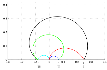
Figure 4: All breaking curves, summarized: they are symmetric about the real $t$–axis. Depending on the case under study, some of them may not be “active”, namely they belong to different sheets of the phase portraits. We refer to Figs. 5, 6, 7, 8, 9, 10 for the specifics.

5.4 Phase portraits or distribution of genera in the complex $t$-plane

There are six different situations depending on the values of $\nu_{j}$’s in the definition of the bilinear form eq. (1-2). Note that only their values up to common multiplication by nonzero constant is relevant, i.e., the orthogonal polynomials are parametrized by points $[\nu_{1}:\nu_{2}:\nu_{3}]\in{\mathbb{C}}\mathbb{P}^{2}$. So, we have:

1. ”Generic” case: $\nu_{j}\neq 0$, $\nu_{1}\neq\nu_{2}$, $\nu_{2}\neq\nu_{3}$;

2. ”Real axis”: $\nu_{2}=\nu_{1}$, $\nu_{3}=0$;

3. ”Single Wedge”: $\nu_{1}=0=\nu_{2}$ ,$\nu_{3}\neq 0$.

4. ”Consecutive Wedges”: $\nu_{3}=0$, $\nu_{2}\neq\nu_{1}$, $\nu_{2}\neq 0$, $\nu_{1}\neq 0$;

5. ”Opposite Wedges, generic”: $\nu_{2}=0$, $\nu_{3}\neq\nu_{1}$, $\nu_{1}\nu_{3}\neq 0$;

6. ”Opposite Wedges, symmetric”: $\nu_{2}=0$, $\nu_{3}=\nu_{1}\neq 0$.

We provide the results of the computer-assisted investigation for all six cases in the tables that follow (Figures 5, 6, 7, 8, 9, 10). The common feature is the following: as we move around the origin $t=0$ counterclockwise the asymptotic directions of the integration contours move clockwise by $\arg(t)/4$. Therefore, a counterclockwise loop around $t=0$ yields a new configuration of contours obtained by a clockwise rotation of $\pi/2$ of the initial one.

In general, thus, we can expect that our phase portraits to have four sheets. In the ”Generic” and ”Opposite Wedges, symmetric” case, however, these four sheets are actually identical, and in the case of ”Real Axis” two of them are equal.

In the pictures that follow the cut (if necessary) is always along the negative $t$-axis and the gluing is the top of the negative axis of sheet $j$ is glued to the bottom of the negative axis of sheet $j+1$ (mod $4$). We hope that the pictorial representation will serve more than many pages of verbal explanation.

We rather explain briefly the algorithm used to investigate the phase portraits; in [2] an algorithm to find numerically ”Boutroux curves” was explained. The algorithm produces a solution of the ”modulation equations” (for branch-points) in high genus, but will not enforce the sign distribution (sign conditions for $h(z)$) needed to have an appropriate $g$-function. In terms of the Remark 4.3 it may yield a signed equilibrium measure. Plotting the level curves allows one to decide unambiguously whether the numerically produced $g$-function satisfies the sign distribution.

The pictures below are produced by some code written in Matlab which is available upon request; the code will allow ”interactive exploration” of the $t$–plane and to produce the pictures interactively.

Remark 5.1 (Zeroes of the orthogonal polynomials)

In all situations considered below, see Figures 5-10, the main arcs consist of all the red arcs that are surrounded by the shaded (light blue) regions on both sides. These arcs, as is well known (see for example [3, 2]), also represent the limiting arcs where the roots of the orthogonal polynomials accumulate, and the (weak) limit of their density can be recovered from the jump of $h^{\prime}(z)$.

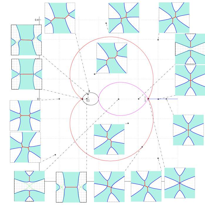
Figure 5: Generic. The region inside the curve joining $\frac{1}{4}$ to $0$ is of genus $1$; inside the curve that joins $t=-\frac{1}{12}$ and $t=0$ it is of genus 0 (symmetric about $z=0$). Everywhere else it is of genus $2$, except for the degeneration to genus $0$ occurring on the curve that joins $t=-\frac{1}{12}$ and $t=\frac{1}{4}$, and to genus $1$ on the ray $[\frac{1}{4},\infty)$. There is a Painlevé I transition at $t=-\frac{1}{12}$ and a Painlevé II transition at $t=\frac{1}{4}$.

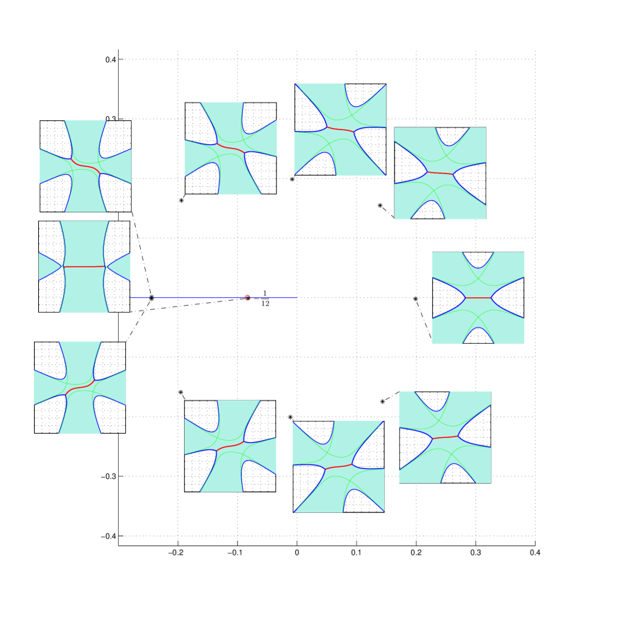
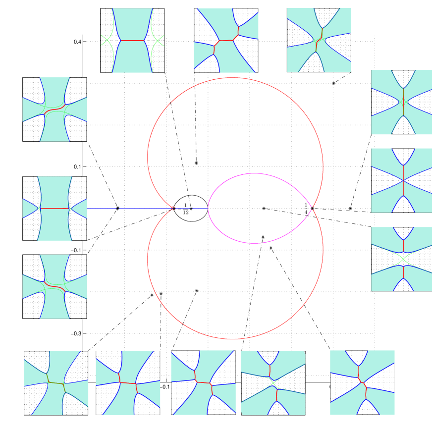
Figure 6: Real Axis. There are two sheets glued along $t\in{\mathbb{R}}_{-}$; the level curves are always symmetric about $z=0$. On the first sheet the solution is always of genus $0$. On the second sheet it is of genus $0$ outside of the curve connecting $t=-\frac{1}{12}$ and $t=\frac{1}{4}$. The region inside the curve joining $\frac{1}{4}$ to $0$ is of genus $1$; inside the curve that joins $t=-\frac{1}{12}$ and $t=0$ it is of genus 0 (symmetric about $z=0$). In the remaining part it is of genus $2$.

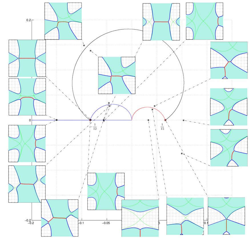
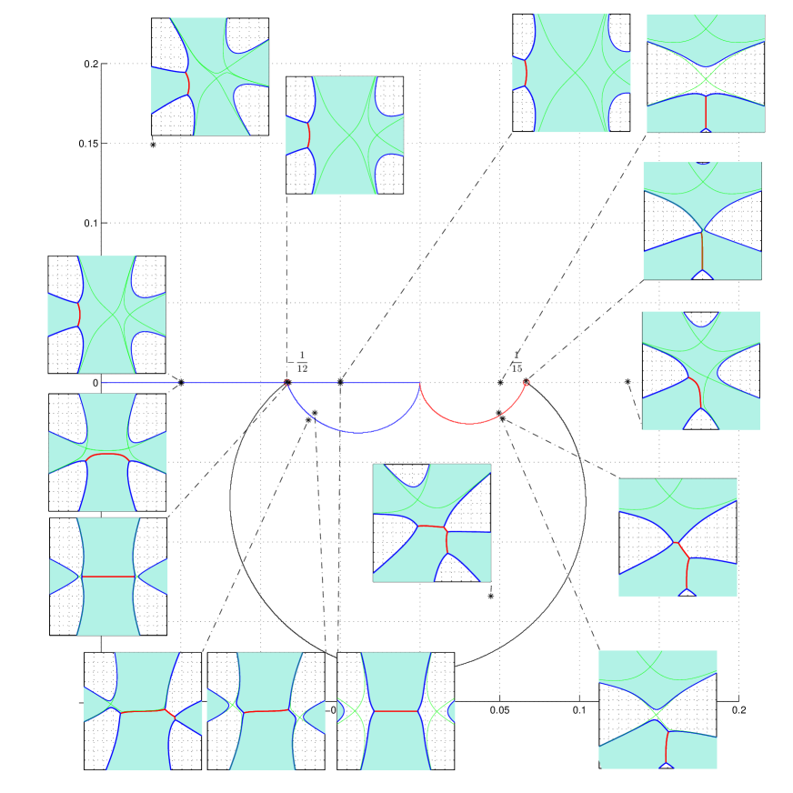
Figure 7: Single Wedge. There are four sheets glued along $t\in{\mathbb{R}}_{-}$; shown here are only sheet $1$ and $2$, because the sheets $3,4$ are copies of sheet $1,2$ where the function $h(z)$ has undergone $z\mapsto-z$. Note that there at the critical point $t=\frac{1}{15}$ on all four sheets we have a transition of type Painlevé I (and also at $t=-\frac{1}{12}$).

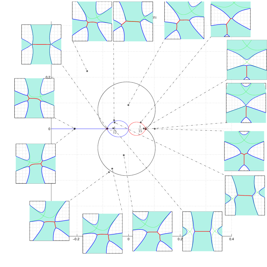
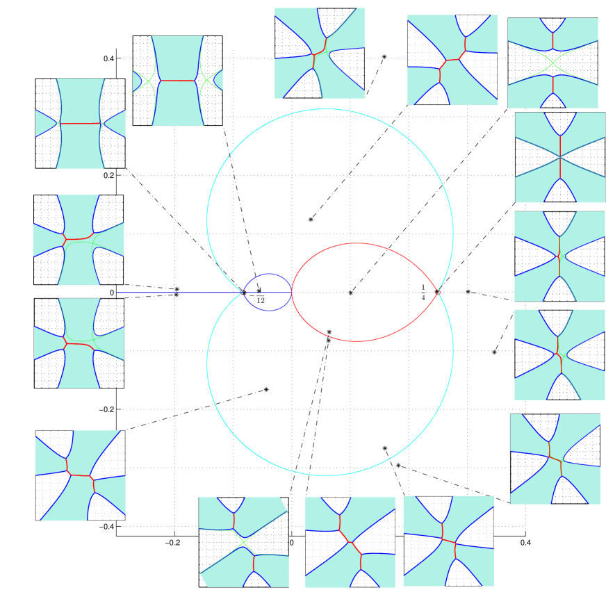
Figure 8: Consecutive Wedges. There are four sheets glued along $t\in{\mathbb{R}}_{-}$; shown here are only sheet $1$ and $2$, because the remaining two sheets are copies of sheet $1$ where the function $h(z)$ has undergone $z\mapsto-z$. Note the Painlevé I transition at both $t=-\frac{1}{12}$ and $t=\frac{1}{15}$.

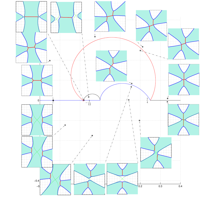
Figure 9: Opposite Wedges, generic. There are two sheets glued along $t\in{\mathbb{R}}_{-}$; shown here are only sheet $1$, because sheet $2$ is a copy of sheet $1$ where the function $h(z;t)$ has undergone $h(z,t)\mapsto\overline{h(\overline{z};\overline{t})}$. Note the Painlevé I transition at $t=-\frac{1}{12}$ and Painlevé II transition at $t=\frac{1}{4}$.

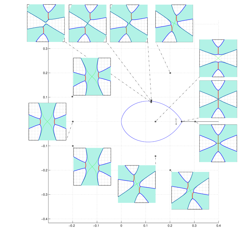
Figure 10: Opposite Wedges, symmetric. There is only one sheet. Note the Painlevé II transition at $t=\frac{1}{4}$. The spectral curve is always of genus $1$ except at the point $t=\frac{1}{4}$.

Remark 5.2

Although the results, presented in Figures 5 - 10 are numerical, there is a straightforward way for their analytic justification. Consider, for example, the Generic case shown in Figures 5. According to Lemma 4.1, the genus zero region contains the interval $(-\frac{1}{12},0)$. Since a break can only occur at one of the curves defined by (5-3), the region contained inside the black curve on Figures 5 is the genus zero region. According to the continuation principle in the parameter space (see [3] and [19]), for any $t$ on the four-sheeted Riemann surface $\Xi$ (with branch-points $t=0$ and $t=\infty$) there exists a contour $\Omega=\mathfrak{M}\cup\mathfrak{C}$ and $h_{n}(z)$, where $\mathfrak{M}$ is the union of all the branch-cuts of $h_{n}$, such that $\Re h_{n}$ satisfies the sign conditions on $\Omega$. Since there are 8 legs of zero level curves of $\Re h$, the genus of the solution for any $t$ cannot be greater than two (as there can be no bounded closed loops of $\Re h=0$). Let us take a point $t_{*}$, $\Im t_{*}>0$, on the main branch $\Lambda$ of the breaking curve (5-3), see Subsection 5.1, that contains genus zero region inside (the curve from $-\frac{1}{12}$ to $0$). Since $t_{*}$ is on the breaking curve, there exists a $z_{*}\in{\mathbb{C}}$, such that the pairs $(t_{*},\pm z_{*})$ satisfy (5-1) (here we use the evenness of $\Re h(z)$). Choose $z_{*}$ so that $\Im z_{*}>0$. If we can show that

$$\Re h_{t}(z_{*};t_{*})>0$$ (5-11)

as $t$ crosses $\Lambda$ along $\Re t=\Re t_{*}$ going up, then we can prove that the genus of $h$ is changing from zero to two as $t$ crosses $\Lambda$. According to the Cauchy-Riemann conditions, (5-11) is equivalent to

$$\Im h_{t}(z_{*};t_{*})<0,$$ (5-12)

where $\Im t=\Im t_{*}$. Using (4-36) and the fact that $1+\frac{t_{*}b^{2}}{2}+t_{*}z_{*}^{2}=0$ (which follows from $h^{\prime}(z_{*};t_{*})=0$), we obtain $z_{*}^{2}=-\frac{1}{t}-\frac{b^{2}}{2}$, so that

$$h_{t}(z_{*};t_{*})=\frac{1}{4t_{*}}\sqrt{\left(-\frac{1}{t_{*}}-\frac{b^{2}}{2}\right)\left(-\frac{1}{t_{*}}-\frac{3b^{2}}{2}\right)}$$ (5-13)

To calculate the branch of the square root in (5-13) we take $t_{*}\rightarrow t_{0}$. As shown in subsection 5.1, in this limit $\arg(t_{*}-t_{0})\rightarrow\frac{2\pi}{5}$, so that, using (4-16), we obtain

$$\arg h_{t}(z_{*};t_{*})\rightarrow\frac{11\pi}{10}.$$ (5-14)

That proves inequality (5-12) when $t_{*}$ is closed to $t_{0}$. Moreover, for any $t_{*}\in\Lambda$ we obtain

$$h_{t}(z_{*};t_{*})=-\frac{1}{4\sqrt{3}t_{*}^{2}}\sqrt{2\sqrt{1+12t_{*}}-(1+12t_{*})}~{}~{}~{}{\rm or}~{}~{}~{}h(u)=-12\frac{\sqrt{6u-u^{2}}}{(u^{2}-1)^{2}},$$ (5-15)

where $u=\sqrt{1+12t_{*}}$. It is easy to see that the upper halfplane part of the genus zero region (between $\Lambda$ and ${\mathbb{R}}$) is contained in the semistrip $0\leq\Re u\leq 1,~{}\Im u\geq 0$ of the $u$-plane. Direct calculations show that: $\Im h(u)=0$ on $[0,1]$, and; $\Im h(u)<0$ on $i{\mathbb{R}}^{+}$, on $1+i{\mathbb{R}}^{+}$ and on any segment $\Im u=y,~{}\Re u\in[0,1]$, where $y>0$ is sufficiently large. Thus, using the maximum principle for $\Im h(u)$ and the fact that $\frac{dh}{du}\neq 0$ on $[0,1]$, we conclude that $\Im h(u)<0$ inside the semistrip. So, we proved the transition from genus zero to genus two across $\Lambda$. Similar considerations will lead to rigorous proofs of transitions through other level curves.

6 Double and multiple scaling analysis near the Painlevé I gradient catastrophe points

Having disposed of the global analysis of the problem in the complex $t$–plane we now focus on the so–called double (and multiple) scaling analysis near the two points of gradient catastrophe that are related to the Painlevé I transcendents. These are

$$t_{0}:=-\frac{1}{12}\ ,\hbox{ and}\ \ t_{1}:=\frac{1}{15}\ .$$ (6-1)

There is another point of gradient catastrophe at $t_{2}:=\frac{1}{4}$ which –however– involves the Painlevé II transcendent and should be analyzed in a separate work.

The two points $t_{0},t_{1}$ can be analyzed much in a parallel fashion: they both necessitate of the same type local parametrix near one -or both- endpoints. The differences between the two cases appear by inspection of the figures: indeed

• near $t=t_{0}$ the genus zero function $h(z;t)=h_{0}(z,t)$ always has symmetric level-curves and hence the Painlevé I parametrix (first introduced in [14]) is needed near both endpoints $\lambda_{0}=-b=-\lambda_{1}$ (see Figs. 5, 6, 7, 8, 9, vignettes near $t_{0}$) ;

• near $t=t_{1}$ the genus zero function $h(z;t)=h_{0}(z,t)$ does not have any special symmetry and the PI parametrix is needed only near one endpoint (see Figs. 5, 6, 7, 8, 9, vignettes near $t_{1}$).

6.1 Local analysis at the point of gradient catastrophe

Near an endpoint the genus-zero $h$–function has necessarily an expansion of the following form

$$\frac{1}{2}h(z) {\hskip-20.0pt}=C_{0}^{(j)}(z-\lambda_{j})^{\frac{3}{2}}+C_{1}^{(j)}(z-\lambda_{j})^{\frac{5}{2}}+C_{2}^{(j)}(z-\lambda_{j})^{\frac{7}{2}}+\cdots=$$ (6-3)

$${\hskip-20.0pt}C_{0}^{(j)}(z-\lambda_{j})^{\frac{3}{2}}\left(1+\frac{C_{1}^{(j)}}{C_{0}^{(j)}}(z-\lambda_{j})+\frac{C_{2}^{(j)}}{C_{0}^{(j)}}(z-\lambda_{j})^{2}+\cdots\right)\ ,\ \ j=0,1,$$

where the coefficients $C_{k}^{(j)}=C_{k}^{(j)}(t)$ depend on $t$. The gradient-catastrophe occurs when the leading coefficient $C_{0}^{(j)}(t)$ vanishes at one or both endpoints $\lambda_{0,1}$ of the main arc $\gamma_{m}$, while (in general) the next coefficient $C_{1}^{(j)}(t)$ does not. For our $f(z,t)$, the gradient catastrophe point is either $t_{0}$ or $t_{1}$. Elementary singularity theory[1] guarantees the validity of the following definition.

Definition 6.1 (Scaling coordinate)

The scaling coordinate $\zeta(z)=\zeta(z;t,N)$ and the exploration parameter $\tau=\tau(t,N)$ are defined by

$$\frac{N}{2}h(z;t)=\frac{4}{5}\zeta^{\frac{5}{2}}{(z;t,N)}+\tau{(t,N)}\zeta^{\frac{3}{2}}{(z;t,N)},$$ (6-4)

where $\zeta(b;t,N)\equiv 0$, $\zeta(z;t,N)$ is analytically invertible in $z$ in a fixed small neighborhood $\mathbb{D}_{j}$ of $z=\lambda_{j}$ and $\tau$ is analytic in $C_{0}^{(j)}$ at $C_{0}^{(j)}=0$, where $j=0,1$.

Let us consider the endpoint $\lambda_{1}$ near the point of gradient catastrophe $t_{*}$, where $t_{*}=t_{0}$ or $t_{*}=t_{0}$. The expression (6-4) is the normal form of the singularity defined by $h(z;x,t)$ (in the sense of singularity theory [1]). The local behaviour (we suppress the superscripts)

$$\zeta = N^{\frac{2}{5}}\left(\frac{5}{4}C_{1}\right)^{\frac{2}{5}}\left(1-\frac{6C_{0}C_{2}}{25C_{1}^{2}}+\mathcal{O}(C_{0}^{2})\right)(z-\lambda_{1})(1+\mathcal{O}(z-\lambda_{1})),$$ (6-5)

$$\tau = N^{\frac{2}{5}}C_{0}\left(\frac{4}{5C_{1}}\right)^{\frac{3}{5}}\left(1+\mathcal{O}(C_{0})\right)$$ (6-6)

was calculated in [5]. The determination of the root is fixed uniquely by the requirement that the image of the main arc $\gamma_{m}$, where $\Re h\equiv 0$, be mapped to the negative real $\zeta$–axis. Following [5], we define:

Definition 6.2

The double scaling near $t=t_{*}$ shall be defined as the appropriate dependence of $t$ such that the variable

$$v=v(t,N):=\frac{3}{8}\tau^{2}(t,N)=\frac{3}{8}N^{\frac{4}{5}}C_{0}^{2}\left(\frac{5}{4}C_{1}\right)^{-\frac{6}{5}}(1+\mathcal{O}(C_{0}))$$ (6-7)

is kept within a disk of arbitrary but fixed (in $N$) radius around $v=0$. The variable $v$ shall be referred to as the Painlevé coordinate.

Near $t_{0}=-\frac{1}{12}$, $\delta t:=t-t_{0}$	Near $t_{1}=\frac{1}{15}$ $\delta t:=t-t_{1}$
$\displaystyle a=0$	$\displaystyle a=-3i\frac{\sqrt{1+\frac{2i}{3}\sqrt{15\delta t}}}{\sqrt{1+15\delta t}}=-3i+\sqrt{15\delta t}+\mathcal{O}(\delta t)$
$\displaystyle b=\frac{\sqrt{8}}{\sqrt{1+\sqrt{12\,\delta t}}}=\sqrt{8}-\frac{\sqrt{8}}{2}\sqrt{12\delta t}+\mathcal{O}(\delta t)$	$\displaystyle b=\frac{2i}{\sqrt{1+i\sqrt{15\delta t}}}=2i+\sqrt{15\delta t}+\mathcal{O}(\delta t)$
$\displaystyle C_{0}=-\frac{1}{6}\left(2+3tb^{2}\right)\sqrt{2b}=-\frac{2\sqrt[4]{2}\sqrt{12\,\delta t}}{3\sqrt[4]{1+\sqrt{12\,\delta t}}}$	$\displaystyle C_{0}=-\frac{1}{3}t\sqrt{2b}a(2a+3b)=\frac{2}{3}{\rm e}^{\frac{3i\pi}{4}}\sqrt{15\delta t}+\mathcal{O}(\delta t)$
$\displaystyle C_{1}=-\frac{19tb^{2}+2}{20\sqrt{2b}}=\frac{\sqrt[4]{1+\sqrt{12\,\delta t}}}{60\sqrt[4]{2}}\left(16-19\sqrt{12\,\delta t}\right)$	$\displaystyle C_{1}=-\frac{1}{5}\frac{t(2a^{2}+15ab+8b^{2})}{2\sqrt{2b}}=\frac{2{\rm e}^{\frac{3i\pi}{4}}}{15}+\mathcal{O}(\sqrt{\delta t})$
$\displaystyle N^{-\frac{2}{5}}\zeta^{\prime}(\lambda_{1})=3^{-\frac{2}{5}}2^{-\frac{1}{10}}+\mathcal{O}(N^{-\frac{2}{5}})$	$\displaystyle N^{-\frac{2}{5}}\zeta^{\prime}(\lambda_{1})=6^{-\frac{2}{5}}{\rm e}^{\frac{3i\pi}{10}}\left(1+\mathcal{O}(N^{-\frac{2}{5}})\right)$
$\displaystyle\frac{\tau}{\zeta^{\prime}(\lambda_{1})}=\frac{4C_{0}}{5C_{1}}(1+\mathcal{O}(C_{0}))=-\sqrt{8}\sqrt{12\delta t}+\mathcal{O}(\delta t)$	$\displaystyle\frac{\tau}{\zeta^{\prime}(\lambda_{1})}=\frac{4C_{0}}{5C_{1}}(1+\mathcal{O}(C_{0}))=4\sqrt{15\delta t}+\mathcal{O}(\delta t)$
$\displaystyle\ell=-\frac{3}{2}+\ln 2-6\delta t+\frac{2}{3}(12\delta t)^{\frac{3}{2}}+\mathcal{O}(\delta t^{2})$	$\displaystyle\ell=\frac{9}{4}+\ln(-1)-\frac{13}{4}(15\delta t)-\frac{2}{3}i(15\delta t)^{\frac{3}{2}}+\mathcal{O}(\delta t^{2})$

Table 2: The explicit expressions and relevant expansions of the indicated quantities: these are the result of straightforward algebraic manipulations using (4-16, 4-20, 4-25, 4-28, 4-30, 4-31, 6-3, 6-4, 6-5, 6-6).

Lemma 6.1

In the double scaling near $t=t_{0}$ for the symmetric genus zero case or near $t=t_{1}$ for the non-symmetric case, the Painlevé coordinate $v$ has the following expansion

$$v(t) {\hskip-20.0pt}=\frac{3}{8}\tau^{2}(t,N)={-3^{\frac{6}{5}}2^{\frac{9}{5}}\left(t+\frac{1}{12}\right)N^{\frac{4}{5}}(1+\mathcal{O}(\sqrt{t-t_{0}}))},\ \ \$$ (6-8)

$$v(t) {\hskip-20.0pt}=\frac{3}{8}\tau^{2}(t,N)=3^{\frac{6}{5}}\,2^{\frac{1}{5}}\,5\,{\rm e}^{\frac{3i\pi}{5}}\left(t-\frac{1}{15}\right)N^{\frac{4}{5}}(1+\mathcal{O}(\sqrt{t-t_{1}}))\ .$$ (6-9)

In either cases the function $v(t)$ is a convergent series in $\sqrt{t-t_{j}}$; if $v$ is kept bounded as $N\to\infty$ then $t-t_{j}=\mathcal{O}(N^{-\frac{4}{5}})$. Therefore from (6-8, 6-9) it follows immediately that with accuracy $\mathcal{O}(N^{-\frac{2}{5}})$ the map $v(t)$ is linear in $\frac{t-t_{j}}{N^{\frac{4}{5}}}$.

The proof is a direct computation with the help of Table 2 and Def. 6.1.

6.2 Asymptotics away from the poles

The asymptotic analysis now depends on the regions in the Painlevé variable $v$ (6-8) or (6-9) that we are investigating. We will split this analysis into the following two cases.

• Away from the poles: the variable $v$ is chosen within a fixed compact set $K$, that does not contain any pole of the relevant solutions to P1;

• Near the poles: the variable $v$ undergoes its own scaling limit and approaches a given pole at a certain rate.

Each of these two cases requires a slightly different analysis depending on the nature of the gradient catastrophe point, be it $t_{0}=-\frac{1}{12}$ or $t_{1}=\frac{1}{15}$. In the former case the analysis was carried out in full in the regime ”Away from the poles” by [10] and the relevant theorem is Thm. 1.1: we will not add anything to it.

The only case that is not covered by the mentioned theorem in the same regime is when $t$ undergoes a double scaling limit near $t_{1}$ and a special Painlevé parametrix is needed only at one endpoint, say, at $\lambda_{1}$. Of course, one may still use the results of [10] with minor modifications to cover this new case, but since we will need some preparatory material, we briefly analyze this case below. We shall construct an approximation to the matrix $\widehat{T}(z;t,N)$ appearing in (4-42) in the form

$$\widehat{T}(z)=\left\{\begin{array}[]{cc}\mathcal{E}(z)\Psi_{0}(z)&\mbox{ for $z$ {\bf outside} of the disks }\mathbb{D}_{1},\mathbb{D}_{0},\\[4.0pt] \mathcal{E}(z)\Psi_{0}(z)\mathcal{P}_{1}(z)&\mbox{ for $z$ {\bf inside} of the disk }\mathbb{D}_{1},\\[4.0pt] \mathcal{E}(z)\Psi_{0}(z)\mathcal{P}_{0}(z)&\mbox{ for $z$ {\bf inside} of the disk }{\mathbb{D}}_{0},\\[4.0pt] \end{array}\right.$$ (6-10)

where $\mathbb{D}_{0},~{}\mathbb{D}_{1}$ are small fixed disks centered at $\lambda_{0}$ and $\lambda_{1}$ respectively, see Fig. 11 and $\Psi_{0}$ as in (4-51). Here $\mathcal{E}(z)$ is the so-called error matrix that will be shown to be close to the identity matrix ${\bf 1}$ and $\mathcal{P}_{0,1}(z)$ are local parametrices at $z=\lambda_{0},\lambda_{1}$, respectively, that will be constructed through the matrix $\Psi(\xi,v)$ defined by (2-6).

Figure 11: The deformation of the contours and the partitioning in complementary (black) and main arcs (blue). Shown also are the lenses and the disks near the two branch-points $\lambda_{1},\lambda_{0}$. The left frame refers to the case $t\sim\frac{1}{15}$, the right frame to $t\sim-\frac{1}{12}$. The thin lines in the shaded area on the left frame are the level-curves passing through the saddle point. For the case on the left ($t=\frac{1}{15}$) we have $\nu_{2}=\nu_{1}\in{\mathbb{C}}$, and $\nu_{3}$ can be normalized to $\nu_{3}=1$; the deformed contour $\varpi_{3}$ consists of the complementary arc on the imaginary axis, the left one and the main arc (thick). The contour $\varpi_{2}+\varpi_{1}$ (homological sum) consists of the two left/right complementary arcs. For the right frame, we have $t={\rm e}^{i\pi}\frac{1}{12}$ and the weights are $\nu_{2}=1$ and $\nu_{1},\nu_{3}\in{\mathbb{C}}$: the contour $\varpi_{1}$ is deformed to go through the two complementary arcs on the bottom and top right, and $\varpi_{2}$ runs along the top right, top left complementary arcs and the main arc, while $\varpi_{3}$ runs along the two complementary arcs on the left. The weights of the various complementary arcs are indicated in the figure and determine the parameters of the Painlevé parametrices to be used according to Definition 2.1. The level-curves in these pictures are numerically accurate.

A local parametrix $\mathcal{P}(z)$ (we drop the indices for convenience) must have a certain number of properties (see Theorem 6.1), one of them being the restriction

$$\mathcal{P}(z)\bigg{|}_{z\in\partial\mathbb{D}}={\bf 1}+o_{\varepsilon}(1)$$ (6-11)

on the boundary of the respective disk $\mathbb{D}$, where $o_{\varepsilon}(1)$ denotes some infinitesimal of $\varepsilon=\frac{1}{N}$, uniformly in $z\in\partial\mathbb{D}$ and in $t\in\hat{K}=v^{-1}(K)$.

If the local parametrices $\mathcal{P}_{0,1}(z)$ satisfying (6-11) can be found then the “error matrix” $\mathcal{E}(z)$ is seen to satisfy a small–norms RHP and, thus, be uniformly close to the identity. More precisely, the matrix $\mathcal{E}$ has jumps on:

1. the parts of the lenses and of the complementary arcs that lie outside of the disks $\mathbb{D}_{0},\mathbb{D}_{1}$, and;

2. on the boundaries of the two disks $\mathbb{D}_{0},\mathbb{D}_{1}$.

The jumps in (a) are exponentially close to the identity in any $L^{p}$ norm (including $L^{\infty}$) while (b) on the boundary of the disks $\mathbb{D}_{0,1}$ we have

$$\mathcal{E}_{+}(z)=\mathcal{E}_{-}(z)\Psi_{0}(z)\mathcal{P}^{-1}_{0,1}(z)\Psi_{0}^{-1}(z)\bigg{|}_{z\in\partial\mathbb{D}_{0,1}}=\mathcal{E}_{-}\left({\bf 1}+o_{\varepsilon}(1)\right).$$ (6-12)

From the analysis in [8] it follows that, for $|z|$ large enough, $\|\mathcal{E}(z)-{\bf 1}\|\leq\frac{o_{\varepsilon}(1)}{|z|}$ (with the pointwise matrix norm) and that the rate of convergence is estimated as the same as the $o_{\varepsilon}(1)$ that appears in (6-11) as $\varepsilon\rightarrow 0$.

In the case at hand we keep in mind that near $t=t_{1}=\frac{1}{15}$ the endpoint $\lambda_{0}$ requires the standard Airy parametrix and that the corresponding error term arising on the boundary of $\mathbb{D}_{0}$ is of order $\mathcal{O}(N^{-1})$.

Definition 6.3 (Local parametrix away from the poles)

Let $\zeta(z;\varepsilon)$ be the local conformal coordinate near $\lambda_{1}$ introduced in Def. 6.1 so that

$$\frac{N}{2}h(z;x,t)=\theta(\zeta;\tau)=\frac{4}{5}\zeta^{\frac{5}{2}}+\tau\zeta^{\frac{3}{2}}\ .$$ (6-13)

Let $\Psi(\xi;v;\varkappa)$ denote the Psi–function of the Painlevé I Problem 2.1 according to Def. 2.1. The parametrix $\mathcal{P}(z;\varkappa)$ is defined by

$$\mathcal{P}(z;\varkappa)=\frac{1}{\sqrt{2}}{\left[\begin{array}[]{cc}1&1\\ i&-i\end{array}\right]}\zeta^{-\frac{\sigma_{3}}{4}}\Psi\left(\zeta+\frac{\tau}{2};\frac{3}{8}\tau^{2};\varkappa\right){\rm e}^{-\theta(\zeta;\tau)\sigma_{3}}\ ,\ \ \ \zeta:=\zeta(z).$$ (6-16)

Theorem 6.1

The matrix $\mathcal{P}_{1}(z):=\mathcal{P}(z;\nu_{1})$ satisfies:

1. Within $\mathbb{D}_{1}$, the matrix $\mathcal{P}_{1}(z)$ solves the exact jump conditions on the lenses and on the complementary arc;

2. On the main arc (cut) $\mathcal{P}_{1}(z)$ satisfies

   $$\mathcal{P}_{1,+}(z)=\sigma_{2}\mathcal{P}_{1,-}(z)\sigma_{2}\ ,$$ (6-17)

   so that $\Psi_{0}\mathcal{P}_{1}$ within $\mathbb{D}_{1}$ solves the exact jumps on all arcs contained therein (the left-multiplier in the jump (6-17) cancels against the jump of $\Psi_{0}$);

3. The product $\Psi_{0}(z)\mathcal{P}_{1}(z)$ (and its inverse) are –as functions of $z$– bounded within $\mathbb{D}_{1}$, namely the matrix $\mathcal{P}_{1}(z)$ cancels the growth of $\Psi_{0}$ at $z=\lambda_{1}$;

4. The restriction of $\mathcal{P}_{1}(z)$ on the boundary of $\mathbb{D}_{1}$ is

   $$\mathcal{P}_{1}(z)\bigg{|}_{z\in\partial\mathbb{D}_{1}}={\bf 1}-\left(H_{I}+\frac{\tau^{3}}{16}\right)\frac{\sigma_{3}}{\sqrt{\zeta}}+\frac{1}{2\zeta}\left[\left(H_{I}+\frac{\tau^{3}}{16}\right)^{2}{\bf 1}+{\left(y+\frac{\tau}{4}\right)}\sigma_{2}\right]+\mathcal{O}(\zeta^{-\frac{3}{2}}),$$ (6-18)

   where $v=\frac{3}{8}\tau^{2}$, $y(v)=y^{(1)}(v)$ and $H_{I}=\frac{1}{2}(y^{\prime})^{2}+yv-2y^{3}=\int y(s){\rm d}s$.

The proof of Theorem 6.1 can be found in Theorem 5.1 of [5] (although it was for the tritronquée solution, the proof is identical for the general case).

6.3 Computation of the correction near $t_{1}$: proof of Theorem 1.2

Proof of Theorem 1.2. According to (6-10), we have

$$\mathcal{E}_{+}=\mathcal{E}_{-}\Psi_{0}\mathcal{P}_{0,1}^{-1}\Psi_{0}^{-1}=\mathcal{E}_{-}\left({\bf 1}+\Delta M(z)\right)~{}~{}{\rm on}~{}~{}\partial\mathbb{D}_{0,1}.$$ (6-19)

In particular, according to (6-18),

$$\Psi_{0}\mathcal{P}_{1}^{-1}\Psi_{0}^{-1}= {\hskip-20.0pt}{\bf 1}+\left(H_{I}+\frac{\tau^{3}}{16}\right)\left(\frac{\sigma_{3}-i\sigma_{1}}{2\sqrt{\zeta p}}+\sqrt{\frac{p}{\zeta}}\frac{\sigma_{3}+i\sigma_{1}}{2}\right)+$$ (6-21)

$${\hskip-20.0pt}+\frac{1}{2\zeta}\left(\left(H_{I}+\frac{\tau^{3}}{16}\right)^{2}{\bf 1}-\left(y+\frac{\tau}{4}\right)\sigma_{2}\right)+\mathcal{O}(N^{-\frac{3}{5}})\ ,\ \ \ p:=\frac{z-\lambda_{1}}{z-\lambda_{0}}.$$

Using ${\bf 1}+\Delta M(z)$ to denote the jump-matrix of $\mathcal{E}$ on all the contours (see below), we can rewrite (6-19) as the integral equation

$$\mathcal{E}(z)={\bf 1}+\frac{1}{2i\pi}\int\frac{\mathcal{E}_{-}(s)\Delta M(s){\rm d}s}{s-z},$$ (6-22)

where the integral is taken along all the jumps of $\mathcal{E}$, that is, along the parts of the lenses and the complementary arcs that lie outside $\mathbb{D}_{0}\cup\mathbb{D}_{1}$ as well as along the boundaries of $\mathbb{D}_{0}$, $\mathbb{D}_{1}$. However, the contribution to $\mathcal{E}$ coming from the integrals along all these contours, except for $\partial\mathbb{D}_{1}$, are of order not exceeding $O(N^{-1})$ (note that the parametrix in $\mathbb{D}_{0}$ is the standard Airy parametrix). Therefore, to obtain the leading order solution, we consider (6-22) with the contour $\partial\mathbb{D}_{1}$. This integral equation will be solved by iterations. The first iteration yields

$$\mathcal{E}^{(1)}(z)={\bf 1}+\frac{1}{\lambda_{1}-z}\left\{\left(H_{I}+\frac{\tau^{3}}{16}\right)\left(\frac{\sigma_{3}-i\sigma_{1}}{2\sqrt{\zeta^{\prime}(\lambda_{1})/(\lambda_{1}-\lambda_{0})}}\right)+\frac{1}{2\zeta^{\prime}(\lambda_{1})}\left(\left(H_{I}+\frac{\tau^{3}}{16}\right)^{2}{\bf 1}-\left(y+\frac{\tau}{4}\right)\sigma_{2}\right)\right\}.$$ (6-23)

Retaining only the terms up to order $\mathcal{O}(N^{-\frac{2}{5}})$ in the second iteration, we obtain

$$\mathcal{E}^{(2)}_{-}(z)=\mathcal{E}^{(1)}_{-}(z)+\mathop{\mathrm{res}}\limits_{s=\lambda_{1}}\left(H_{I}+\frac{\tau^{3}}{16}\right)^{2}\left(\frac{\sigma_{3}-i\sigma_{1}}{2\sqrt{\zeta^{\prime}(\lambda_{1})/(\lambda_{1}-\lambda_{0})}}\right)\frac{1}{(\lambda_{1}-s)(s-z)}\left(\sqrt{\frac{p(s)}{\zeta(s)}}\frac{\sigma_{3}+i\sigma_{1}}{2}\right){\rm d}s=$$ (6-24)

$$={\bf 1}+\frac{\mathcal{E}^{(1)}_{1}}{\lambda_{1}-z}-\left(H_{I}+\frac{\tau^{3}}{16}\right)^{2}\left(\frac{1}{\zeta^{\prime}(\lambda_{1})}\right)\frac{1}{\lambda_{1}-z}\left(\frac{{\bf 1}-\sigma_{2}}{2}\right)=$$ (6-25)

$$={\bf 1}+\frac{1}{\lambda_{1}-z}\left\{\left(H_{I}+\frac{\tau^{3}}{16}\right)\left(\frac{\sigma_{3}-i\sigma_{1}}{2\sqrt{\zeta^{\prime}(\lambda_{1})/(\lambda_{1}-\lambda_{0})}}\right)-\frac{1}{2\zeta^{\prime}(\lambda_{1})}\left(y+\frac{\tau}{4}-\left(H_{I}+\frac{\tau^{3}}{16}\right)^{2}\right)\sigma_{2}\right\}.$$ (6-26)

Therefore, using the fact that $\lambda_{1}=a+b,\ \lambda_{0}=a-b$, we have

$$T(z)=\left({\bf 1}+\frac{E_{1}}{\lambda_{1}-z}+\mathcal{O}(N^{-\frac{3}{5}})\right)\left({\bf 1}-\frac{(\lambda_{1}-\lambda_{0})\sigma_{2}}{4z}+\frac{(\lambda_{1}-\lambda_{0})^{2}-4(\lambda_{1}^{2}-\lambda_{0}^{2})\sigma_{2}}{32z^{2}}\right)=$$ (6-27)

$$={\bf 1}-\frac{2E_{1}+b\sigma_{2}}{2z}-\frac{(a+b)E_{1}}{z^{2}}+\frac{bE_{1}\sigma_{2}}{2z^{2}}+\frac{b^{2}-4ab\sigma_{2}}{8z^{2}}.$$ (6-28)

From this we can read off the relevant matrix entries:

$$(T_{1})_{22} {\hskip-20.0pt}=\frac{\left(H_{I}+\frac{\tau^{3}}{16}\right)}{\sqrt{2\zeta^{\prime}(\lambda_{1})/b}}=:{\bf G},$$ (6-29)

$$(T_{1})_{12} {\hskip-20.0pt}=i{\bf G}+\frac{ib}{2}-\frac{i}{2\zeta^{\prime}(\lambda_{1})}\left(y+\frac{\tau}{4}\right)+\frac{i}{b}{\bf G}^{2},$$ (6-30)

$$(T_{1})_{21} {\hskip-20.0pt}=i{\bf G}-\frac{ib}{2}+\frac{i}{2\zeta^{\prime}(\lambda_{1})}\left(y+\frac{\tau}{4}\right)-\frac{i}{b}{\bf G}^{2},$$ (6-31)

$$(T_{2})_{12} {\hskip-20.0pt}=\frac{iab}{2}-(a+b)\left[i{\bf G}+\frac{i}{2\zeta^{\prime}(\lambda_{1})}\left(y+\frac{\tau}{4}\right)-\frac{i}{b}{\bf G}^{2}\right]-\frac{ib{\bf G}}{2},$$ (6-32)

where all the terms have accuracy $\mathcal{O}(N^{-\frac{3}{5}})$. Direct computation using (4-48) shows

$$\alpha_{n}=\frac{b^{2}}{4}-\frac{b}{2\zeta^{\prime}(\lambda_{1})}\left(y+\frac{\tau}{4}\right)+\mathcal{O}(N^{-\frac{3}{5}})\ ,\ \ \ \beta_{n}=a-\frac{y+\frac{\tau}{4}}{\zeta^{\prime}(\lambda_{1})}+\mathcal{O}(N^{-\frac{3}{5}}).$$ (6-33)

Using Table 2, we see that

$$a=a_{0}+\frac{\tau}{4\zeta^{\prime}(\lambda_{1})}+\mathcal{O}(N^{-\frac{4}{5}})\ ,\ \ \ b=b_{0}+\frac{\tau}{4\zeta^{\prime}(\lambda_{1})}+\mathcal{O}(N^{-\frac{4}{5}}),$$ (6-34)

where $a_{0}=-3i$, $b_{0}=2i$, and, thus

$$\alpha_{n}=\frac{b_{0}^{2}}{4}-\frac{b_{0}}{2\zeta^{\prime}(\lambda_{1})}y+\mathcal{O}(N^{-\frac{3}{5}})=-1+\frac{i6^{\frac{2}{5}}{\rm e}^{-\frac{3i\pi}{10}}}{N^{\frac{2}{5}}}y(v)+\mathcal{O}(N^{-\frac{3}{5}}),$$ (6-35)

$$\beta_{n}=a_{0}-\frac{y}{\zeta^{\prime}(\lambda_{1})}+\mathcal{O}(N^{-\frac{3}{5}})=-3i-\frac{6^{\frac{2}{5}}{\rm e}^{-\frac{3i\pi}{10}}}{N^{\frac{2}{5}}}y(v)+\mathcal{O}(N^{-\frac{3}{5}}).$$ (6-36)

To compute ${\mathbf{h}}_{n}$ we use (4-48). Noticing that ${\bf G}=\mathcal{O}(N^{-\frac{1}{5}})$, we can rearrange $(T_{1})_{12}$ as follows:

$$(T_{1})_{12}=\frac{ib_{0}}{2}-\frac{iy}{2\zeta^{\prime}(\lambda_{1})}+i{\bf G}+\frac{i}{b_{0}}{\bf G}^{2}+\mathcal{O}(N^{-\frac{3}{5}})=\frac{ib_{0}}{2}\left(1-\frac{y}{b_{0}\zeta^{\prime}(\lambda_{1})}+\frac{2{\bf G}}{b_{0}}+\frac{2{\bf G}^{2}}{b_{0}^{2}}+\mathcal{O}(N^{-\frac{3}{5}})\right)$$ (6-37)

$$=\frac{ib_{0}}{2}\left(1-\frac{y}{b_{0}\zeta^{\prime}(\lambda_{1})}\right){\rm e}^{\frac{2{\bf G}}{b_{0}}}(1+\mathcal{O}(N^{-\frac{3}{5}})).$$ (6-38)

Therefore

$${\mathbf{h}}_{n}=-2i\pi(T_{1})_{12}{\rm e}^{N\ell}=\pi b_{0}\left(1-\frac{y}{b_{0}\zeta^{\prime}(\lambda_{1})}\right){\rm e}^{N\ell+\frac{2{\bf G}}{b_{0}}}(1+\mathcal{O}(N^{-\frac{3}{5}})).$$ (6-39)

Utilizing (6-29) and the values in Table 2 we find:

$${\hskip-20.0pt}{\mathbf{h}}_{n}=2i\pi\left(1-\frac{y}{2i\zeta^{\prime}(\lambda_{1})}\right)\exp\left[N\ell-i\left(\frac{H_{I}}{\sqrt{-i\zeta^{\prime}(\lambda_{1})}}+\frac{\tau^{3}}{16\zeta^{\prime}(\lambda_{1})^{3}\sqrt{-i}}(\zeta^{\prime}(\lambda_{1})^{5})^{\frac{1}{2}}\right)\right](1+\mathcal{O}(N^{-\frac{3}{5}}))$$ (6-40)

$${\hskip-20.0pt}=2i\pi\left(1-\frac{y}{2i\zeta^{\prime}(\lambda_{1})}\right)\exp\left[N\ell-i\left(\frac{H_{I}}{\sqrt{-i\zeta^{\prime}(\lambda_{1})}}-\frac{4(15\delta t)^{\frac{3}{2}}}{\sqrt{-i}}\frac{N}{6}{\rm e}^{-\frac{i\pi}{4}}\right)\right](1+\mathcal{O}(N^{-\frac{3}{5}}))$$ (6-41)

$${\hskip-20.0pt}=2i\pi(-1)^{N}\left(1-\frac{{\rm e}^{-\frac{4}{5}i\pi}}{3^{-\frac{2}{5}}2^{\frac{3}{5}}}\frac{y(v)}{N^{\frac{2}{5}}}\right)\exp\left[\frac{9N}{4}-\frac{13N}{4}(15\delta t)-N\frac{2}{3}i(15\delta t)^{\frac{3}{2}}-i\left({\rm e}^{\frac{1}{10}i\pi}\frac{6^{\frac{1}{5}}H_{I}}{N^{\frac{1}{5}}}-\frac{2N}{3}(15\delta t)^{\frac{3}{2}}\right)\right]$$ (6-42)

$${\hskip-20.0pt}(1+\mathcal{O}(N^{-\frac{3}{5}}))$$ (6-43)

$$=2i\pi(-1)^{N}\left(1-\frac{3^{\frac{2}{5}}}{2^{\frac{3}{5}}}{\rm e}^{-\frac{4}{5}i\pi}\frac{y(v)}{N^{\frac{2}{5}}}\right)\exp\left[\frac{9N}{4}-\frac{195N}{4}\delta t+{\rm e}^{-\frac{2}{5}i\pi}\frac{6^{\frac{1}{5}}}{N^{\frac{1}{5}}}H_{I}\right](1+\mathcal{O}(N^{-\frac{3}{5}})).$$ (6-44)

Q.E.D.

7 Analysis near the poles: triple scaling limit

The analysis in [10] was carried through under the assumption that –in the double scaling limit– the Painlevé coordinate is chosen in an arbitrary compact set that does not contain any of the poles of the functions $y^{(0)},y^{(1)}$ (see Theorem 1.1). Our special interest now is the analysis in the vicinity of anyone of such poles.

To set the stage in general terms, we shall consider the case where the Painlevé variable $v$ undergoes its own scaling. If $v_{p}$ is the pole under scrutiny, we shall consider the following triple scaling limit, whereby, in addition to $N\rightarrow\infty$ and $N^{\frac{4}{5}}(t-t_{*})$ being bounded, we also impose

$$v-v_{p}=\mathcal{O}\left(N^{-\frac{1}{5}-\rho}\right),$$ (7-1)

where $\rho\geq 0$ (depending on the situation, it may be bounded above).

There are two distinct scenarios depending on whether the coalescence of the saddle points (zeroes of $h^{\prime}(z)$) with the branch-points $\lambda_{0,1}$ occurs at both branch-points or only at one, say, at $\lambda_{1}$. These scenarios corresponds to the analysis near the critical points $t_{0}=-\frac{1}{12}$, and $t_{1}=\frac{1}{15}$ respectively. We recall that $t_{0}=\frac{1}{12}$ is a point of gradient catastrophe in all the situations discussed in Sect. 5.4, with the exception of situation ”Opposite Wedges, symmetric” (Fig. 10). Viceversa, the gradient catastrophe point $t_{1}=\frac{1}{15}$ occurs only in ”Single Wedge” (Fig. 7) and ”Consecutive Wedges” (Fig. 8).

7.1 The asymmetric case

Under this title we treat both the case where $t$ is near $t_{1}$ (which requires a special parametrix only near one endpoint, say $\lambda_{1}$, and the standard Airy parametrix near the other) and the case of $t$ near $t_{0}$ but with $\nu_{1}\neq{1-\nu_{3}}$ The latter case requires some special parametrix at both endpoints; but a given value of $v$, generically, can be near the pole of only one of the two special solution $y^{(0)}(v),~{}y^{(1)}(v)$ of the Painlevé I equation that enter in Theorem 1.1. Below, we assume that $v$ is close to the pole $v_{p}$ of $y^{(1)}(v)$. The case when a pole $v_{p}$ of $y^{(1)}(v)$ is simultaneously a pole of $y^{(0)}(v)$ even though $\nu_{1}\neq{1-\nu_{3}}$ and, thus, $y^{(0)}\not\equiv y^{(1)}$, could be treated as the symmetric case (Subsection 7.2) with minor modifications (but we shall not consider it here for simplicity).

We define the approximate solution to the RHP (4-2) with the jump matrix (4-43) as

$$\Phi(z)=\left\{\begin{array}[]{cc}E(z)\Psi_{0}(z)&\mbox{ for $z$ {\bf outside} of the disks }\mathbb{D}_{0},\mathbb{D}_{1}\\[4.0pt] E(z)\Psi_{0}(z)\mathcal{P}_{0}(z)&\mbox{ for $z$ {\bf inside} of the disk }\mathbb{D}_{0},\\[4.0pt] E(z)\Psi_{0}(z)\hat{\mathcal{P}}_{1}(z)&\mbox{ for $z$ {\bf inside} of the disk }{\mathbb{D}}_{1}.\\[4.0pt] \end{array}\right.$$ (7-2)

where the matrix $E(z)$, discussed below, is needed to “adjust” the situation due to the pole $v_{p}$. Here the parametrix $\mathcal{P}_{0}(z)$ is the Airy parametrix if we are near $t_{1}$. If we are near $t_{0}$, the parametrix $\mathcal{P}_{0}(z)$ is given by

$$\mathcal{P}_{0}(z):=\sigma_{3}\mathcal{P}(-z;1-\nu_{3})\sigma_{3},$$ (7-3)

where $\mathcal{P}(z;\varkappa)$ was introduced in Definition 6.3. To introduce the parametrix $\hat{\mathcal{P}}_{1}(z)$, we first define $\widehat{\Psi}$ by the Masoero factorization ([17])

$$\Psi(\xi;v;\varkappa)=(\xi-y)^{-\sigma_{3}/2}\left[\begin{array}[]{cc}\frac{1}{2}\left(y^{\prime}+\frac{1}{2(\xi-y)}\right)&1\\ 1&0\end{array}\right]\widehat{\Psi}(\xi;v;\varkappa)$$ (7-4)

with $\Psi$ as in Def. 6.3 and $y=y(v;\varkappa)$ (prime denotes derivative in $v$).

Definition 7.1 (Local parametrix near the poles.)

The parametrix $\widehat{\mathcal{P}}_{1}(z)$ is defined in $\mathbb{D}_{1}$ as

$$\widehat{\mathcal{P}}_{1}(z)=\widehat{\mathcal{P}}_{1}(z;\nu_{1})=\frac{1}{\sqrt{2}}\left[\begin{array}[]{cc}i&i\\ -1&1\end{array}\right]\zeta^{\frac{3}{4}{\sigma_{3}}}\widehat{\Psi}\left(\zeta+\frac{\tau}{2};\frac{3}{8}\tau^{2};\nu_{1}\right){\rm e}^{-\theta(\zeta;\tau)\sigma_{3}},$$ (7-7)

where $\zeta(z;\varepsilon)$ is the local conformal coordinate in $\mathbb{D}_{1}$, see Definition 6.3. We can then formulate the statement corresponding to Theorem 6.1 for the new local parametrix.

Theorem 7.1 (Theorem 6.1 in [5])

The matrix $\widehat{\mathcal{P}}_{1}$ satisfies:

1. Within $\mathbb{D}_{1}$, the matrix $\widehat{\mathcal{P}}_{1}(z)$ solves the exact jump conditions on the lenses and on the complementary arcs;

2. On the main arc (cut) $\widehat{\mathcal{P}}_{1}(z)$ satisfies

   $$\widehat{\mathcal{P}}_{1+}(z)=\sigma_{2}\widehat{\mathcal{P}}_{1-}(z)\sigma_{2}\ ,$$ (7-8)

   so that $\Psi_{0}\widehat{\mathcal{P}}_{1}$ within $\mathbb{D}_{1}$ solves the exact jumps on all arcs contained therein (the left-multiplier in the jump (7-8) cancels against the jump of $\Psi_{0}$);

3. The product $\Psi_{0}(z)(z-\lambda_{1})^{-\sigma_{2}}\widehat{\mathcal{P}}_{1}(z)$ (and its inverse) are –as functions of $z$– bounded within $\mathbb{D}_{1}$, namely the matrix $\widehat{\mathcal{P}}_{1}(z)$ cancels the growth of $\Psi_{0}(z)(z-\lambda_{1})^{-\sigma_{2}}$ at $z=\lambda_{1}$;

4. The restriction of $\widehat{\mathcal{P}}_{1}(z)$ on the boundary of $\mathbb{D}_{1}$ is

   $$\widehat{\mathcal{P}}_{1}(z)\bigg{|}_{z\in\partial\mathbb{D}_{\alpha}}=\left({\bf 1}+\mathcal{O}(\zeta^{-\frac{1}{2}})\right)\left(\frac{\sqrt{1-\zeta/y}}{1+\sqrt{\zeta/y}}\right)^{-\sigma_{3}},$$ (7-9)

   where $\mathcal{O}(\zeta^{-\frac{1}{2}})$ is uniform w.r.t. $v$ in a small, compact neighborhood of a pole $v_{p}$ that does not contain any zero of $y(v)$.

The statements in [5] were tailored to the case of the tritronquée solution and there was a slightly different normalization, but the proof goes through in identical fashion. Also note that the parametrix in [5] differs from $\widehat{\mathcal{P}}_{1}$ by a conjugation by $\sigma_{2}$.

7.1.1 Triple scaling: proof of Theorem 1.3

Before delving into the proof we make some preparatory remarks: first off, recall that we are choosing $v$ so that $v-v_{p}=\mathcal{O}(N^{-\frac{1}{5}-\rho})$, $\rho\geq 0$; this means that $y(v)=\frac{1}{(v-v_{p})^{2}}+\mathcal{O}(v-v_{p})^{2}$ also grows at a rate $y(v)=\mathcal{O}(N^{\frac{2}{5}+2\rho})$. Recall also that for $z\in\partial\mathbb{D}_{1}$ we have $\zeta(z)=\mathcal{O}(N^{\frac{2}{5}})$; therefore

$$\frac{\zeta(z)}{y(v)}=\mathcal{O}(N^{-2\rho}),\ \ \ \ z\in\partial\mathbb{D}_{1},\ \rho\geq 0.$$ (7-10)

In the case $\rho=0$ the disk around $\lambda_{1}$ shall be chosen sufficiently small so that $|\zeta/y|<1-\delta$ for some $\delta>0$; this means that the rightmost factor in (7-9) is a uniformly smooth and bounded matrix on $\partial\mathbb{D}_{1}$. In fact it also tends to the identity if $\rho>0$, but in general it does so very slowly (in $N$) or not at all (if $\rho=0$, which is the most interesting case). Therefore we can move the rightmost factor in (7-9) to the left at “no cost”. So, we can write

$$\hat{\mathcal{P}}_{1}(z)\bigg{|}_{z\in\partial\mathbb{D}_{1}}=\left({\bf 1}+\mathcal{O}(\zeta^{-\frac{1}{2}})\right)\left(\frac{\sqrt{1-\zeta/y}}{1+\sqrt{\zeta/y}}\right)^{-\sigma_{3}}=\left(\frac{\sqrt{1-\zeta/y}}{1+\sqrt{\zeta/y}}\right)^{-\sigma_{3}}\left({\bf 1}+\mathcal{O}(\zeta^{-\frac{1}{2}})\right).$$ (7-11)

If $\rho=0$, the above mentioned factor does not tend to identity.

We require that the approximate solution $\Phi(z)$ from (7-2) satisfies

$$\Phi(z)=\left\{\begin{array}[]{cc}\Phi_{+}(z)=\Phi_{-}(z)({\bf 1}+o(1))&\mbox{ uniformly in $z$ on }\partial\mathbb{D}_{0}\cup\partial\mathbb{D}_{1}\\[4.0pt] \Phi(z)&\mbox{is bounded for $z$ { inside} the disks $\mathbb{D}_{0}\cup\mathbb{D}_{1}$},\\[4.0pt] \end{array}\right.$$ (7-12)

In particular, in view of point 3 in Theorem 7.1, the requirements of (7-12) will become true if the matrix $E(z)$, introduced in (7-2), would satisfy the following RHP problem for $E(z)$.

Problem 7.1

$$\left\{\begin{array}[]{cc}E_{+}(z)=E_{-}(z)\Psi_{0}(z)\left(\frac{\sqrt{1-\zeta/y}}{1+\sqrt{\zeta/y}}\right)^{\sigma_{3}}\Psi^{-1}_{0}(z)&\mbox{ on }\partial\mathbb{D}_{1},\\[4.0pt] E(z)=O(1)(z-\lambda_{1})^{-\sigma_{3}}(\sigma_{2}+\sigma_{3})&\mbox{ as }z\rightarrow\lambda_{1},\\[4.0pt] E(z)={\bf 1}+O(\frac{1}{z})&\mbox{ as }z\rightarrow\infty,\end{array}\right.$$ (7-13)

where $O(1)$ means an invertible matrix analytic at $z=\lambda_{1}$, bounded together with its inverse, and the circle $\partial\mathbb{D}_{1}$ has positive orientation.

Note that the second condition of (7-13) is equivalent to

$$E(z)\Psi_{0}(z)\left[\begin{array}[]{cc}i&i\\ -1&1\end{array}\right]\zeta(z)^{\frac{3}{4}\sigma_{3}}=O(1)\qquad\mbox{ as }z\rightarrow\lambda_{1},$$ (7-14)

given that $\zeta(z)=\mathcal{O}(z-\lambda_{1})$. Equation (7-14) together with Theorem 7.1, item 3, guarantee the boundedness of

$$\Phi(z)=E(z)\Psi_{0}(z)\hat{\mathcal{P}}_{1}(z)=\underbrace{E(z)\Psi_{0}(z)\frac{1}{\sqrt{2}}{\left[\begin{array}[]{cc}i&i\\ -1&1\end{array}\right]}\zeta^{\frac{3}{4}{\sigma_{3}}}}_{=\mathcal{O}(1)}\overbrace{\widehat{\Psi}\left(\zeta+\frac{\tau}{2};\frac{3}{8}\tau^{2}\right){\rm e}^{-\theta(\zeta;\tau)\sigma_{3}}}^{=\mathcal{O}(1)},$$ (7-15)

within the disc $\mathbb{D}_{1}$.

Proof of solution of the Problem 7-13

Let $\widehat{E}(z)=\frac{1}{2}(\sigma_{2}+\sigma_{3})E(z)(\sigma_{2}+\sigma_{3})$. Then

$$\left\{\begin{array}[]{cc}\widehat{E}_{+}(z)=\widehat{E}_{-}(z)M(z)&\mbox{ on }\partial\mathbb{D}_{1},\\[4.0pt] \widehat{E}(z)=O(1)(z-\lambda_{1})^{-\sigma_{3}}&\mbox{ as }z\rightarrow\lambda_{1},\\[4.0pt] \widehat{E}(z)={\bf 1}+O(\frac{1}{z})&\mbox{ as }z\rightarrow\infty,\\[4.0pt] \end{array}\right.$$ (7-16)

where

$$M=\frac{1}{2}(\sigma_{2}+\sigma_{3})\Psi_{0}\left(\frac{\sqrt{1-\zeta/y}}{1+\sqrt{\zeta/y}}\right)^{\sigma_{3}}\Psi_{0}^{-1}(\sigma_{2}+\sigma_{3}).$$ (7-17)

Using (4-51) and the fact that

$$S^{\sigma_{2}}=e^{\ln S\sigma_{2}}=\cosh(\ln S\sigma_{2})+\sinh(\ln S\sigma_{2})=\frac{1}{2}(S+S^{-1}){\bf 1}+\frac{1}{2}(S-S^{-1})\sigma_{2},$$ (7-18)

we calculate

$$M(z)=[A(z),B(z)]=\frac{1}{\sqrt{1-\frac{\zeta}{y}}}\left({\bf 1}+i\sqrt{\frac{\zeta p}{y}}\sigma_{+}-i\sqrt{\frac{\zeta}{py}}\sigma_{-}\right),\ {\rm where}~{}~{}p:=\frac{z-\lambda_{1}}{z-\lambda_{0}}$$ (7-19)

and $\sigma_{\pm}=\frac{1}{2}(\sigma_{1}\pm i\sigma_{2})$. We make the Ansatz that $\widehat{E}_{-}(z)={\bf 1}+\frac{L}{z-\lambda_{1}}$: then the (constant in $z$) matrix $L$ must be chosen so that $\widehat{E}_{+}(z)=\widehat{E}_{-}(z)M(z)$ satisfies

$$\widehat{E}_{+}(z)(z-\lambda_{1})^{\sigma_{3}}=\left({\bf 1}+\frac{L}{z-\lambda_{1}}\right)[A,B](z-\lambda_{1})^{\sigma_{3}}=\mathcal{O}(1),~{}~{}~{}z\in\mathbb{D}_{1}.$$ (7-20)

In light of (6-5) we see that $A(\lambda_{1})=\mathcal{O}(1)$, and thus we need to consider only the second column of (7-20):

$$\left({\bf 1}+\frac{L}{z-\lambda_{1}}\right)\frac{B(z)}{z-\lambda_{1}}=\frac{B(z)}{z-\lambda_{1}}+\frac{LB(z)}{(z-\lambda_{1})^{2}}=\mathcal{O}(1)$$ (7-21)

or

$$\left\{\begin{array}[]{cc}LB(\lambda_{1})=0&\\[4.0pt] B(\lambda_{1})+LB^{\prime}(\lambda_{1})=0.&\\[4.0pt] \end{array}\right.$$ (7-22)

Calculating

$$B(\lambda_{1})=(0,1)^{T}\ ,\qquad B^{\prime}(\lambda_{1})=\left(i\sqrt{\frac{\zeta^{\prime}(\lambda_{1})}{2by}},\frac{\zeta^{\prime}(\lambda_{1})}{2y}\right)^{T},$$ (7-23)

we see that

$$L=i\sqrt{\frac{(\lambda_{1}-\lambda_{0})y}{\zeta^{\prime}(\lambda_{1})}}\sigma_{-}$$ (7-24)

solves the system (7-22). Thus

$$\left\{\begin{array}[]{cl}\displaystyle\widehat{E}_{-}(z)&=\displaystyle{\bf 1}+i\frac{\sqrt{\frac{y(\lambda_{1}-\lambda_{0})}{\zeta^{\prime}(\lambda_{1})}}\sigma_{-}}{z-\lambda_{1}},\\[9.0pt] \displaystyle\widehat{E}_{+}(z)&=\left({\bf 1}+i\frac{\sqrt{\frac{y(\lambda_{1}-\lambda_{0})}{\zeta^{\prime}(\lambda_{1})}}\sigma_{-}}{z-\lambda_{1}}\right)M(z)\end{array}\right.$$ (7-25)

solves the RHP (7-16). Since $\frac{i}{2}(\sigma_{2}+\sigma_{3})\sigma_{-}(\sigma_{2}+\sigma_{3})=\frac{1}{2}(\sigma_{3}-i\sigma_{1})$, we obtain that

$$\left\{\begin{array}[]{cl}\displaystyle E_{-}(z)&\displaystyle={\bf 1}{+}\frac{\sqrt{\frac{y(\lambda_{1}-\lambda_{0})}{\zeta^{\prime}(\lambda_{1})}}(\sigma_{3}-i\sigma_{1})}{2(z-\lambda_{1})},\\[9.0pt] \displaystyle E_{+}(z)&\displaystyle=\left({\bf 1}{+}\frac{\sqrt{\frac{y(\lambda_{1}-\lambda_{0})}{\zeta^{\prime}(\lambda_{1})}}(\sigma_{3}-i\sigma_{1})}{2(z-\lambda_{1})}\right)\Psi_{0}\left(\frac{\sqrt{1-\zeta/y}}{1+\sqrt{\zeta/y}}\right)^{\sigma_{3}}\Psi_{0}^{-1}\end{array}\right.$$ (7-26)

solves the RHP (7-13). Q.E.D.

Error analysis.

The error matrix $\mathcal{E}(z)=T(z)\Phi^{-1}(z)$ has jumps on the lenses and on the complementary arcs outside the disks $\mathbb{D}_{0},\mathbb{D}_{1}$, as well as on the boundary of these disks. The jump matrices on the lenses and on the complementary arcs approach ${\bf 1}$ exponentially fast in $N^{-1}$ and uniformly in $z$. It is also clear that $\mathcal{E}\rightarrow{\bf 1}$ as $z\rightarrow\infty$ since both $T$ and $\Phi=E\Psi_{0}$ do so. So, it remains only to prove the uniform convergence to ${\bf 1}$ of the jump matrix on $\partial\mathbb{D}_{1}$ (convergence on $\partial\mathbb{D}_{0}$ was established in Subsection 6.2). Indeed, using (7-2), (7-13), (7-9), (7-11) and (7-26), we have

$$\mathcal{E}_{+} {\hskip-20.0pt}=T\Phi_{+}^{-1}=T\hat{\mathcal{P}}^{-1}_{1}\Psi^{-1}_{0}E^{-1}_{+}=T\Phi^{-1}_{-}E_{-}\Psi_{0}\hat{\mathcal{P}}^{-1}_{1}\Psi^{-1}_{0}\Psi_{0}\left(\frac{\sqrt{1-\zeta/y}}{1+\sqrt{\zeta/y}}\right)^{-\sigma_{3}}\Psi^{-1}_{0}E^{-1}_{-}$$ (7-28)

$${\hskip-20.0pt}=\mathcal{E}_{-}E_{-}\Psi_{0}({\bf 1}+\mathcal{O}(\zeta^{-1/2}))\Psi^{-1}_{0}E^{-1}_{-}=\mathcal{E}_{-}E_{-}({\bf 1}+\mathcal{O}(\zeta^{-1/2}))E^{-1}_{-}.$$

On the boundary $z\in\partial\mathbb{D}_{1}$ we have $\zeta=\mathcal{O}(N^{\frac{2}{5}})$ and in our triple scaling $y=\mathcal{O}(N^{\frac{2}{5}+2\rho})$ with $\rho\geq 0$. Then $L$ is of the order $\mathcal{O}(N^{-\frac{1}{5}}\sqrt{y})=\mathcal{O}(N^{\rho})$. Thus,

$$E_{-}\mathcal{O}(\zeta^{-1/2})E^{-1}_{-}=\mathcal{O}(\zeta^{-1/2})+\frac{[L,\mathcal{O}(\zeta^{-1/2})]}{z-\lambda_{1}}-\frac{L\mathcal{O}(\zeta^{-1/2})L}{(z-\lambda_{1})^{2}}=\mathcal{O}(N^{-\frac{1}{5}})+\mathcal{O}(N^{-\frac{1}{5}+\rho})+\mathcal{O}(N^{-\frac{1}{5}+2\rho}).$$ (7-29)

So, it is the last term that contributes the slowest decay. Therefore, we obtain

$$\mathcal{E}_{+}=\mathcal{E}_{-}({\bf 1}+\mathcal{O}(N^{-\frac{3}{5}}y)),~{}~{}~{}~{}~{}z\in\partial\mathbb{D}_{1}.$$ (7-30)

The latter estimate shows that we can control the error provided

$$y=y^{(1)}=O(N^{\frac{2}{5}+\rho}),~{}~{}~{}{\rm or,~{}equivalently,~{}}~{}~{}v-v_{p}=O(N^{-\frac{1}{5}-\rho}),$$ (7-31)

where $0\leq\rho<\frac{1}{5}$.

Computation of the recurrence coefficients:

We need to use (3-19) and (7-30). Using (7-2), (7-26) and the expansion of $\Psi_{0}$ (4-52) we obtain

$$\Phi(z) {\hskip-20.0pt}=\displaystyle E_{-}(z)\Psi_{0}(z)=\left({\bf 1}{+}\frac{1}{2}\frac{k{(\sigma_{3}-i\sigma_{1})}}{z-\lambda_{1}}\right)\left({\bf 1}-\frac{b}{2z}\sigma_{2}+\frac{b^{2}}{8z^{2}}{\bf 1}-\frac{ab\sigma_{2}}{2z^{2}}+O(z^{-3})\right)$$ (7-35)

$${\hskip-20.0pt}=\left({\bf 1}+\frac{1}{2}k{(\sigma_{3}-i\sigma_{1})}\left(\frac{1}{z}+\frac{\lambda_{1}}{z^{2}}\right)\right)\left({\bf 1}-\frac{b}{2z}\sigma_{2}+\frac{b^{2}}{8z^{2}}{\bf 1}-\frac{ab\sigma_{2}}{2z^{2}}+O(z^{-3})\right)$$

$${\hskip-20.0pt}={\bf 1}+\frac{1}{z}\left[\frac{k}{2}\left(\sigma_{3}-i\sigma_{1}\right)-\frac{b}{2}\sigma_{2}\right]+\frac{1}{z^{2}}\left[\frac{b^{2}{\bf 1}}{8}-\frac{ab}{2}\sigma_{2}+\frac{k}{2}\left(a+\frac{1}{2}b\right)\left(\sigma_{3}-i\sigma_{1}\right)\right]$$

$${\hskip-20.0pt}\displaystyle k:=\sqrt{\frac{(\lambda_{1}-\lambda_{0})y}{\zeta^{\prime}(\lambda_{1})}}=\sqrt{\frac{2by}{\zeta^{\prime}(\lambda_{1})}}$$

We introduce

$$s:=\sqrt{\frac{\zeta^{\prime}(\lambda_{1})}{2by(v)}}=\sqrt{\frac{\zeta^{\prime}(\lambda_{1})}{2b_{0}}}(v-v_{p})+\mathcal{O}\left(N^{\frac{1}{5}}(v-v_{p})^{5}\right),$$ (7-36)

where the latter expression follows from (1-15). Here and henceforth $a_{0},b_{0}$ denote the values of $a,b$ calculated exactly at one of the critical points $t_{0}$ or $t_{1}$. Assuming in $\rho=0$ in (7-31), we obtain $s=\mathcal{O}(1)$ as $N\rightarrow\infty$. On the other hand, if $\rho\in(0,\frac{1}{5})$, then, consequently, $s$ scales as $\mathcal{O}(N^{-\rho})$. Thus, we have the triple scaling limit

$$t-t_{j}=\frac{v}{\kappa N^{\frac{4}{5}}}=\frac{v_{p}}{\kappa N^{\frac{4}{5}}}+\frac{\sqrt{\frac{2b_{0}}{\zeta^{\prime}(\lambda_{1})}}}{\kappa N^{\frac{4}{5}}}s,$$ (7-37)

where $\kappa$ is the constant in front of $\delta t=t-t_{j}$ appearing in formulæ (6-8, 6-9). Explicitly, using Table 2, we obtain

$$t+\frac{1}{12}=-\frac{v_{p}}{3^{\frac{6}{5}}2^{\frac{9}{5}}N^{\frac{4}{5}}}-\frac{s}{3\sqrt{2}N}\ ,\qquad t-\frac{1}{15}=\frac{v_{p}{\rm e}^{-\frac{3i\pi}{5}}}{3^{\frac{6}{5}}2^{\frac{1}{5}}5N^{\frac{4}{5}}}-i\frac{2s}{15N}.$$ (7-38)

Now, according to (4-48), (4-30), (4-31) and (7-30), we obtain:

$$\alpha_{n} {\hskip-20.0pt}=(T_{1})_{12}(T_{1})_{21}=\frac{b^{2}}{4}{-}\frac{by(v)}{2N^{\frac{2}{5}}C}+\mathcal{O}(N^{-\frac{3}{5}}y)=\frac{b_{0}^{2}}{4}-\frac{1}{4s^{2}}+\mathcal{O}(N^{-\frac{3}{5}}y,N^{-\frac{2}{5}}),$$ (7-39)

$$\beta_{n} {\hskip-20.0pt}=\frac{\left(T_{2}\right)_{12}}{\left(T_{1}\right)_{12}}-\left(T_{1}\right)_{22}=a_{0}+\frac{1}{2s(1-b_{0}s)+\mathcal{O}(N^{-\frac{3}{2}}y)}+\mathcal{O}(N^{-\frac{3}{2}}y,N^{-\frac{2}{5}}),$$ (7-40)

$${\mathbf{h}}_{n} {\hskip-20.0pt}=-2i\pi(T_{1})_{12}{\rm e}^{N\ell}=\left[\pi\left(b_{0}-\frac{1}{s}\right)+\mathcal{O}(N^{-\frac{3}{2}}y,N^{-\frac{2}{5}})\right]{\rm e}^{\left[N\ln\frac{b^{2}}{4}-N\frac{2a^{2}+b^{2}}{8}-\frac{N}{2}\right]}.$$ (7-41)

Here $\mathcal{O}(N^{-\frac{2}{5}})$ error term comes from replacing $a,b$ with their respective values $a_{0},b_{0}$ considered at the critical point $t_{0}$ or $t_{1}$. Note, however, that in the regime (7-1), the $\mathcal{O}(N^{-\frac{2}{5}})$ term is of a smaller order than the $\mathcal{O}(N^{-\frac{3}{2}}y)$ term. Therefore, in all these expressions, in the regime (7-1), the error is at best $\mathcal{O}(N^{-\frac{1}{5}})$ (recall that $y=\mathcal{O}(N^{\frac{2}{5}+2\rho})$ $\rho\in[0,\frac{1}{5})$). Thus in the exponent ${\rm e}^{N\ell}$ we can use the expansion in Table 2 up to order $\delta t$ included. So,

$${\mathbf{h}}_{n}=\pi\left(\frac{b_{0}^{2}}{4}\right)^{N}\exp\left[-N\frac{2a_{0}^{2}+b_{0}^{2}+4}{8}+cN\delta t\right]\left(b_{0}-\frac{1}{s}+\mathcal{O}(N^{-\frac{3}{2}}y)\right),$$ (7-42)

where $c=-6$ for the case $t\sim t_{0}$ and $c=-\frac{13\cdot 15}{4}$ for the case $t\sim t_{1}$. One has then to replace $\delta t$ by the expressions in (7-38). So, in the leading order,

$${\mathbf{h}}_{n} {\hskip-20.0pt}=\pi\left(\sqrt{8}-\frac{1}{s}\right)2^{N}\exp\left[-\frac{3N}{2}+\frac{N^{\frac{1}{5}}v_{p}}{3^{\frac{1}{5}}2^{\frac{4}{5}}}+\sqrt{2}\,{s}\right]\ ,\ \ \ t\sim-\frac{1}{12},$$ (7-43)

$${\mathbf{h}}_{n} {\hskip-20.0pt}=\pi\left(2i-\frac{1}{s}\right)(-1)^{N}\exp\left[\frac{9N}{4}-\frac{13}{4}\frac{N^{\frac{1}{5}}v_{p}{\rm e}^{-\frac{3i\pi}{5}}}{3^{\frac{1}{5}}2^{\frac{1}{5}}}+i\frac{13}{2}s\right]\ ,\ \ \ t\sim\frac{1}{15}.$$ (7-44)

It is remarkable to note that the genus zero leading order asymptotics $\alpha_{n}(t)\sim\frac{b^{2}}{4}$ and $\beta_{n}(t)\sim a$ are valid as long $y=o(N^{\frac{2}{5}})$ with the accuracy $O(\frac{y}{N^{\frac{2}{5}}})$. However, when $y=O(N^{\frac{2}{5}})$, both terms in (7-39), (7-40), contribute to the leading order, whereas, when $y=O(N^{\frac{2}{5}+2\rho})$ with $\rho\in[0,\frac{1}{5})$, the asymptotics are determined by the latter terms of (7-39), (7-40). In this case, both $\alpha_{n}$ and $\beta_{n}$ are unbounded as $N\rightarrow\infty$.

So, the proof of Theorem 1.3 is completed. Q.E.D.

7.2 The symmetric case: proof of Theorem 1.4

We are now in the symmetric situation and hence the critical point to consider can only be $t_{0}=-\frac{1}{12}$, where $\lambda_{1}=b$, $\lambda_{0}=-b$ and $a\equiv 0$. This case is significantly different from the previous inasmuch as the two Painlevé parametrices in $\mathbb{D}_{0,1}$ are identical: in particular $y^{(1)}=y^{(0)}=y$. Thus, if the double scaling is such that we are close to a pole $v_{p}$ of $y(v)$, this will simultaneously affect the both parametrices and, as we shall see, will have a significant effect on the asymptotics of $\alpha_{n}$. On the other hand, due to the exact symmetry of the bilinear pairing, the orthogonal polynomials have the same parity of their degree and thus automatically $\beta_{n}\equiv 0$.

It will be advantageous for us to use a different solution to the model problem (4-50), which has a different growth rate near the branch-points: such modification (see [11]) is called a discrete Schlesinger transformation. In terms of the RHP (4-50), this amounts to replacing the solution $\Psi_{0}$ (4-51) with

$$\Psi_{1}(z):=\frac{1}{2}(\sigma_{3}+\sigma_{2})\left(\frac{z-b}{z+b}\right)^{-\frac{3}{4}\sigma_{3}}(\sigma_{3}+\sigma_{2})=\left(\frac{z-b}{z+b}\right)^{-\frac{3}{4}\sigma_{2}}.$$ (7-45)

This matrix satisfies all the conditions of the RHP (4-50) except the last one, as it clearly has a different growth behaviour near the endpoints $\pm b$. We then shall construct an approximate solution

$$\Phi(z)=\left\{\begin{array}[]{cc}E(z)\Psi_{1}(z)&\mbox{ for $z$ {\bf outside} of the disks }\mathbb{D}_{0},\mathbb{D}_{1}\\[4.0pt] E(z)\Psi_{1}(z)\widehat{\mathcal{P}}_{0}(z)&\mbox{ for $z$ {\bf inside} of the disk }\mathbb{D}_{0},\\[4.0pt] E(z)\Psi_{1}(z)\hat{\mathcal{P}}_{1}(z)&\mbox{ for $z$ {\bf inside} of the disk }{\mathbb{D}}_{1},\\[4.0pt] \end{array}\right.$$ (7-46)

where $\hat{\mathcal{P}}_{1}(z)$ is defined by (7-7) and

$$\widehat{\mathcal{P}}_{0}(z)=\sigma_{3}\widehat{\mathcal{P}}_{1}(-z)\sigma_{3}\ .$$ (7-47)

Due to the fact that we are using $\Psi_{1}$ instead of $\Psi_{0}$, the boundedness of the product $\Psi_{1}\widehat{\mathcal{P}}_{0,1}$ at $\lambda_{0},\lambda_{1}$ follows immediately (see also Theorem 7.1, item 3). Hence, the requirements on the left multiplier $E(z)$ are now different compare with the asymmetric case studied above (we reuse the same symbol $E$ with a new meaning relative to the previous section).

Problem 7.2

Find the matrix $E(z)$ is analytic (together with its inverse) on ${\mathbb{C}}\setminus(\partial\mathbb{D}_{0}\cup\partial\mathbb{D}_{1})$ and satisfies

$$\left\{\begin{array}[]{cc}E_{+}(z)=E_{-}(z)\Psi_{1}(z)\left(\frac{\sqrt{1-\zeta/y}}{1+\sqrt{\zeta/y}}\right)^{\sigma_{3}}\Psi^{-1}_{1}(z)&\mbox{ on }\partial\mathbb{D}_{0,1},\\[4.0pt] E(z)={\bf 1}+\mathcal{O}(\frac{1}{z})&\mbox{ as }z\rightarrow\infty,\end{array}\right.$$ (7-48)

where the contours $\partial\mathbb{D}_{0,1}$ have positive orientation.

Proof of solution of Problem 7.2. Note that any solution to this RHP has unit determinant and hence its inverse is also analytic and bounded. As before, we find it more convenient to solve the RHP for $\widehat{E}(z)=FE(z)F$ instead of the RHP (7-48). Here $F=\frac{\sigma_{2}+\sigma_{3}}{\sqrt{2}}$. The jump matrix for the new RHP is

$$M(z)=F^{-1}\Psi_{1}(z)Q^{-1}(z)\Psi_{1}^{-1}(z)F,$$ (7-49)

where

$$Q:=\left(\frac{\sqrt{1-\zeta/y}}{1+\sqrt{\zeta/y}}\right)^{-\sigma_{3}},$$ (7-50)

$y=y(v)$, $v$ was defined by (6-8) and the local scaling coordinate $\zeta=\zeta(z,N)$ near $z=b$ was introduced in (6-5).

Direct calculations yield

$$M(z)=\frac{1}{\sqrt{1-\zeta(z)/y}}\left[\begin{array}[]{cc}1&i\sqrt{\frac{\zeta(z)(z+b)^{3}}{y(z-b)^{3}}}\\ -i\sqrt{\frac{\zeta(z)(z-b)^{3}}{y(z+b)^{3}}}&1\end{array}\right].$$ (7-51)

Similarly, near $z=-b$ we obtain

$$\tilde{M}(z)=\frac{1}{\sqrt{1-\tilde{\zeta}(z)/y}}\left[\begin{array}[]{cc}1&i\sqrt{\frac{\tilde{\zeta}(z)(z+b)^{3}}{y(z-b)^{3}}}\\ -i\sqrt{\frac{\tilde{\zeta}(z)(z-b)^{3}}{y(z+b)^{3}}}&1\end{array}\right],$$ (7-52)

$${\rm where}~{}~{}~{}~{}~{}\tilde{\zeta}=\tilde{\zeta}(z)=\zeta(-z)\ ,\ \ z\in\mathbb{D}_{0}.$$ (7-53)

Note that the orthogonal polynomials in this case are even/odd and the symmetry of the RHP implies (which can be verified directly from the above formulæ and also as a consequence of (7-49))

$$\Psi_{1}(z)=\sigma_{3}\Psi_{1}(-z)\sigma_{3}\ \ \Rightarrow\ \ \ \widetilde{M}(z)=\sigma_{2}M(-z)\sigma_{2}$$ (7-54)

Using (7-51), (7-52), (6-5), (7-53), we obtain

$$M(z)-{\bf 1}=\frac{\eta\sigma_{+}}{z-b}+O_{1}(z),~{}~{}~{}~{}\tilde{M}(z)-{\bf 1}=\frac{\eta\sigma_{-}}{z+b}+O_{0}(z),$$ (7-55)

where

$$\eta=iN^{\frac{1}{5}}\sqrt{\frac{(2b)^{3}C}{y}}.$$ (7-56)

Here $C=N^{-\frac{2}{5}}\tilde{\zeta}^{\prime}(b)$ and $\tilde{C}=N^{-\frac{2}{5}}\tilde{\zeta}^{\prime}(-b)=-C$ by the symmetry of the problem. Note that the $O_{0,1}$ terms in (7-55) are analytic at $z=\lambda_{0,1}$ and when evaluated at $z=\lambda_{0,1}=\pm b$ are proportional to $\sigma_{\pm}$ (respectively). The matrix $\widehat{E}(z)$ satisfies

$$\widehat{E}(z)={\bf 1}+\oint_{|s-b|=r}\!\!\!\!\frac{\widehat{E}_{-}(s)(M(s)-{\bf 1})}{s-z}\frac{{\rm d}s}{2i\pi}+\oint_{|s+b|=r}\!\!\!\!\frac{\widehat{E}_{-}(s)(\tilde{M}(s)-{\bf 1})}{s-z}\frac{{\rm d}s}{2i\pi}.$$ (7-57)

We pose the Ansatz

$$\widehat{E}_{-}(z)={\bf 1}+\frac{A}{z-b}+\frac{\tilde{A}}{z+b},$$ (7-58)

and obtain

$$\frac{A}{z-b}+\frac{\tilde{A}}{z+b}=-\frac{A\eta\sigma_{+}}{(z-b)^{2}}-\frac{\eta\sigma_{+}}{z-b}-\frac{\tilde{A}\eta\sigma_{+}}{2b(z-b)}-\frac{\tilde{A}\eta\sigma_{-}}{(z+b)^{2}}-\frac{AO_{1}(b)}{z-b}-\frac{\tilde{A}O_{0}(-b)}{z+b}-\frac{\eta\sigma_{-}}{z+b}-\frac{A\eta\sigma_{-}}{2b(z+b)}.$$ (7-59)

That leads to the following system for the unknown $A,\tilde{A}$ (recall that $O_{1}(b)\propto\sigma_{+},\ O_{0}(-b)\propto\sigma_{-}$):

$$A\sigma_{+}=0, \tilde{A}\sigma_{-}=0,$$ (7-60)

$$A+\frac{\eta}{2b}\tilde{A}\sigma_{+}=-\eta\sigma_{+}, \tilde{A}+\frac{\eta}{2b}A\sigma_{-}=-\eta\sigma_{-}.$$ (7-61)

This system has the solution

$$A=\frac{1}{1+\frac{\eta^{2}}{(2b)^{2}}}\left[\begin{array}[]{cc}0&-\eta\\ 0&\frac{\eta^{2}}{{2b}}\end{array}\right],~{}~{}~{}~{}~{}~{}~{}\tilde{A}=-\frac{1}{1+\frac{\eta^{2}}{(2b)^{2}}}\left[\begin{array}[]{cc}\frac{\eta^{2}}{{2b}}&0\\ \eta&0\end{array}\right]=-\sigma_{2}A\sigma_{2}$$ (7-66)

So, we found $\widehat{E}(z)$ and, thus, $E(z)$. Note that the function $E(z)$ in the region outside of the disks is a rational function with poles at $\pm b$, while, inside the disks, it is analytic and given by formula (7-57). Q.E.D.

Error analysis.

The error matrix $\mathcal{E}(z)=T(z)\Phi^{-1}(z)$ has jumps on the lenses and on the complementary arcs outside the disks $\mathbb{D}_{0},\mathbb{D}_{1}$, as well as on the boundary of these disks. The jump matrices on the lenses and on the complementary arcs approach ${\bf 1}$ exponentially fast in $N$ and uniformly in $z$. It is also clear that $\mathcal{E}\rightarrow{\bf 1}$ as $z\rightarrow\infty$. So, it remains only to prove the uniform convergence to ${\bf 1}$ of the jump matrix on $\partial\mathbb{D}_{0,1}$: the computations are absolutely parallel and we report only the one for $\partial\mathbb{D}_{1}$. Using (7-2), the solution to Problem 7.2 and eq. (7-9), we have

$$\mathcal{E}_{+} {\hskip-20.0pt}=T\Phi_{+}^{-1}=T\hat{\mathcal{P}}^{-1}_{1}\Psi^{-1}_{1}E^{-1}_{+}=T\Phi^{-1}_{-}E_{-}\Psi_{1}\hat{\mathcal{P}}^{-1}_{1}\Psi^{-1}_{1}\Psi_{1}\left(\frac{\sqrt{1-\zeta/y}}{1+\sqrt{\zeta/y}}\right)^{-\sigma_{3}}\Psi^{-1}_{1}E^{-1}_{-}$$ (7-68)

$${\hskip-20.0pt}=\mathcal{E}_{-}E_{-}\Psi_{1}({\bf 1}+\mathcal{O}(\zeta^{-1/2}))\Psi^{-1}_{1}E^{-1}_{-}=\mathcal{E}_{-}E_{-}({\bf 1}+\mathcal{O}(\zeta^{-1/2}))E^{-1}_{-}.$$

On the boundary $z\in\partial\mathbb{D}_{1}$ we have $\zeta=\mathcal{O}(N^{\frac{2}{5}})$ and in our double scaling $y=\mathcal{O}(N^{\frac{2}{5}+2\rho})$, where $\rho\in[0,\frac{1}{5})$. Moreover, $E_{-}={\bf 1}+\frac{FAF}{z-b}+\frac{F\tilde{A}F}{z+b},$ where $A,\tilde{A}$ are of the same order. That creates the situation that is drastically different from the previous: for example, the matrices $A,\tilde{A}$ (7-66) remain bounded no matter how fast $y$ grows (and hence $\eta\to 0$ (7-56)). The only unboundedness occurs when the denominators in (7-66) vanish, which means that $\eta$ has a finite value $\eta^{2}=-4b^{2}$ or, equivalently,

$$N^{-\frac{2}{5}}y(v)=2Cb.$$ (7-69)

Condition (7-69) identifies two points near the pole $v=v_{p}$ at a distance of order $\mathcal{O}(N^{-\frac{1}{5}})$. Thus, in (7-68) we have

$$E_{-}\mathcal{O}(\zeta^{-1/2})E^{-1}_{-}=\mathcal{O}(\zeta^{-1/2})+\mathcal{O}\left(\zeta^{-\frac{1}{2}}\left(1+\frac{\eta^{2}}{4b^{2}}\right)^{-1}\right)=\mathcal{O}(N^{-\frac{1}{5}})+\mathcal{O}\left(N^{-\frac{1}{5}}\left(1+\frac{\eta^{2}}{4b^{2}}\right)^{-1}\right)$$ (7-70)

The very last contribution to the error term comes from the denominators of the matrices $A,\tilde{A}$ (7-66) and prevents us from getting close “too fast” to the points where they vanish.

Computation of the recurrence coefficients:

Following [5], we find the expansion of the matrix $\Phi(z)=E(z)\Psi_{1}(z)$ at $z=\infty$:

$$E\Psi_{1}=F\hat{E}(z)\left(\frac{z-b}{z+b}\right)^{-\frac{3}{4}\sigma_{3}}F^{-1}={\bf 1}+\frac{F(A+\tilde{A})F^{-1}+\frac{3}{2}b\sigma_{2}}{z}+\frac{\frac{b}{2}F(\tilde{A}-A)F^{-1}+\frac{9}{8}b^{2}{\bf 1}}{z^{2}}+O(z^{-3}).$$ (7-71)

Using (7-66), we obtain

$$\tilde{A}+A=-\frac{1}{1+\frac{\eta^{2}}{(2b)^{2}}}\left(\frac{\eta^{2}}{2b}\sigma_{3}+\eta\sigma_{1}\right),~{}~{}~{}~{}~{}~{}\tilde{A}-A=-\frac{1}{1+\frac{\eta^{2}}{(2b)^{2}}}\left(\frac{\eta^{2}}{2b}{\bf 1}-i\eta\sigma_{2}\right),$$ (7-72)

so that

$${\hskip-20.0pt}F(\tilde{A}+A)F^{-1}=\frac{1}{1+\frac{\eta^{2}}{(2b)^{2}}}\left[-\frac{\eta^{2}}{2b}\sigma_{2}+\eta\sigma_{1}\right]\ ,\qquad F(\tilde{A}-A)F^{-1}=\frac{1}{1+\frac{\eta^{2}}{(2b)^{2}}}\left[-\frac{\eta^{2}}{2b}{\bf 1}+i\eta\sigma_{3}\right].$$ (7-74)

It follows from (7-71) and (7-74) that the residue of $\Phi$ at infinity, which we denote by $\Phi_{1}$, is

$$\Phi_{1}=F(A+\widetilde{A})F^{-1}+\frac{3}{2}b\sigma_{2}=b\frac{1}{1+\frac{\eta^{2}}{4b^{2}}}\left(\left(-\frac{\eta^{2}}{2b^{2}}\sigma_{2}+\frac{\eta}{b}\sigma_{1}\right)+\frac{3}{2}\left(1+\frac{\eta^{2}}{4b^{2}}\right)\sigma_{2}\right)=$$ (7-75)

$$=b\frac{1}{1+\frac{\eta^{2}}{4b^{2}}}\left(\left(-\frac{\eta^{2}}{8b^{2}}\sigma_{2}+\frac{\eta}{b}\sigma_{1}\right)+\frac{3}{2}\sigma_{2}\right)$$ (7-76)

We note in passing that $\Phi_{1}$ is off-diagonal and $\Phi_{2}$ is diagonal (which implies $\beta_{n}=0$, which -of course- is identity and not just an approximation due to the special symmetry of this case). Then

$$(\Phi_{1})_{12}=\frac{b}{2}\frac{-3i+\frac{i\eta^{2}}{4b^{2}}+2\frac{\eta}{b}}{1+\frac{\eta^{2}}{(2b)^{2}}}=-i\frac{b}{2}\frac{3+\frac{i\eta}{2b}}{1-\frac{i\eta}{2b}}$$ (7-77)

$$(\Phi_{1})_{21}=\frac{b}{2}\frac{3i-\frac{i\eta^{2}}{4b^{2}}+2\frac{\eta}{b}}{1+\frac{\eta^{2}}{(2b)^{2}}}=i\frac{b}{2}\frac{3-\frac{i\eta}{2b}}{1+\frac{i\eta}{2b}}$$ (7-78)

Using (7-70), we can now calculate the (leading order) final expressions

$$\alpha_{n}=(T_{1})_{12}(T_{1})_{21}=\frac{b^{2}}{4}\frac{9+\frac{\eta^{2}}{4b^{2}}}{1+\frac{\eta^{2}}{4b^{2}}}\!\!\!,\quad\beta_{n}=0$$ (7-79)

where it is understood that both expressions (also in the denominators) are affected by an error of the order indicated in (7-70). Introducing

$$s=-\frac{i\eta}{2b}=N^{\frac{1}{5}}\sqrt{\frac{8b^{3}C}{y}},$$ (7-80)

we note that $\mathcal{O}(N^{-\frac{1}{5}}(1+\eta^{2}/(4b^{2}))^{-1})=\mathcal{O}(N^{-\frac{1}{5}}(s^{2}-1)^{-1})$ and we find finally (using Table 2 for the symmetric case)

$$\alpha_{n} {\hskip-20.0pt}=\frac{b^{2}}{4}\frac{9-s^{2}+\mathcal{O}(N^{-\frac{1}{5}})}{1-s^{2}+\mathcal{O}(N^{-\frac{1}{5}})},\qquad\beta_{n}=0,$$ (7-81)

$${\mathbf{h}}_{n} {\hskip-20.0pt}=2^{N}\pi\sqrt{8}\exp\left[-\frac{3N}{2}-6N^{\frac{1}{5}}\frac{\delta t}{N^{-\frac{4}{5}}}\right]\left(\frac{3-s}{1+s}+\mathcal{O}\left(\frac{N^{-\frac{1}{5}}}{1-s^{2}}\right)\right).$$ (7-82)

Using (6-8) and Table 2 to relate $s$ and $t$, we can write (7-82) as

$${\mathbf{h}}_{n}=\pi\sqrt{8}\,2^{N}\exp\left[-\frac{3N}{2}+\frac{N^{\frac{1}{5}}\,v_{p}}{3^{\frac{1}{5}}2^{\frac{4}{5}}}-\frac{s}{4}\right]\left(\frac{3-s}{1+s}+\mathcal{O}\left(\frac{N^{-\frac{1}{5}}}{1-s^{2}}\right)\right).$$ (7-83)

Q.E.D.

References

- [1] V. I. Arnol’d, S. M. Guseĭn-Zade and A. N. Varchenko, Singularities of differentiable maps. Vol. I, volume 82 of Monographs in Mathematics. Birkhäuser Boston Inc., Boston, MA, 1985. The classification of critical points, caustics and wave fronts, Translated from the Russian by Ian Porteous and Mark Reynolds.
- [2] M. Bertola, Boutroux curves with external field: equilibrium measures without a minimization problem arXiv:0705.3062, submitted.
- [3] M. Bertola and M. Y. Mo, Commuting difference operators, spinor bundles and the asymptotics of orthogonal polynomials with respect to varying complex weights. Advances in Mathematics.220(1):154-218, 2009.
- [4] M. Bertola, Moment determinants as isomonodromic tau functions. Nonlinearity.22(1):29–50, 2009.
- [5] M. Bertola and A. Tovbis, Universality for the focusing Nonlinear Schrödinger equation at gradient catastrophe point: Rational breathers and poles of the tritronquée solution to Painlevé I. submitted, see also arXiv:1004.1828.
- [6] T.S.Chihara, An introduction to orthogonal polynomials. Gordon and Breach Science Publishers 1978.
- [7] P. A. Deift, Orthogonal polynomials and random matrices, : a Riemann-Hilbert approach. volume 3 of Courant Lecture Notes in Mathematics NYU, Courant Institute of Mathematical Sciences, New York, 1999.
- [8] P. Deift, T. Kriecherbauer, K. T.-R. McLaughlin, S. Venakides, and X. Zhou, Uniform asymptotics for polynomials orthogonal with respect to varying exponential weights and applications to universality questions in random matrix theory. Comm. Pure Appl. Math., 52(11):1335–1425, 1999.
- [9] P. Deift and X. Zhou, A steepest descent method for oscillatory Riemann-Hilbert problems. Bull. Amer. Math. Soc. (N.S.), 26(1):119–123, 1992.
- [10] M. Duits and and A.B.J. Kuijlaars, Painlevé I asymptotics for orthogonal polynomials with respect to a varying quartic weight. Nonlinearity 19:2211–2245, 2006.
- [11] M. Jimbo and T. Miwa, Monodromy preserving deformation of linear ordinary differential equations with rational coefficients. II. Phys. D, 2(3):407–448, 1981.
- [12] M. Jimbo and T. Miwa, Monodromy preserving deformation of linear ordinary differential equations with rational coefficients. III. Phys. D, 4(1):26–46, 1981/82.
- [13] M. Jimbo, T. Miwa, and K. Ueno, Monodromy preserving deformation of linear ordinary differential equations with rational coefficients. I. General theory and -function. Phys. D, 2(2):306–352, 1981.
- [14] A.S. Fokas, A.R. Its, and A.V. Kitaev, The isomonodromy approach to matrix models in 2D quantum gravity. Comm. Math. Phys., 147 (1992), 395–430.
- [15] G. Freud, On the coefficients in the recursion formulæ of orthogonal polynomials Proc. Roy. Irish Acad. Sect A 76 (1976), no. 1, 1-6.
- [16] A. A. Kapaev, Quasi-linear stokes phenomenon for the Painlevé first equation. J. Phys. A, 37(46):11149–11167, 2004.
- [17] D. Masoero, Poles of integrale tritronquee and anharmonic oscillators. A WKB approach. J. Phys. A: Math. Theor., 43(095201), 09 2010.
- [18] G. Szego, Orthogonal polynomials. AMS Colloquium Publications, Vol. XXIII 1975.
- [19] A. Tovbis and S. Venakides, Nonlinear steepest descent asymptotics for semiclassical limit of integrable systems: Continuation in the parameter space. Comm. Math. Phys.,, 295(1):139–160, 2010.
- [20] A. Tovbis, S. Venakides, and X. Zhou. On semiclassical (zero dispersion limit) solutions of the focusing nonlinear Schrödinger equation. Comm. Pure Appl. Math., 57(7):877–985, 2004.
- [21] A. Tovbis, S. Venakides, and X. Zhou, Semiclassical focusing nonlinear Schrödinger equation I: inverse scattering map and its evolution for radiative initial data. Int. Math. Res. Not. IMRN, (22):Art. ID rnm094, 54, 2007.