Critical analysis of a variational method used to describe the molecular electron transport

Abstract

In a recent paper [I. Bâldea and H. Köppel, Phys. Rev. B78, 115315 (2008)], we showed that a variational approach [P. Delaney and J. C. Greer, Phys. Rev. Lett. 93, 036805 (2004)] proposed to compute the electron transport through molecules, which is based on boundary constraints of the Wigner function, is unable to correctly describe the zero-bias conductance of the simplest uncorrelated and correlated systems. In the present paper, we extend our previous analysis of the linear response limit of that approach, by considering, instead of the Wigner function, general constraints. We demonstrate that, if, as usual in transport theories, the quasi-particle distributions in electrodes are constrained, this method yields the completely unphysical result that the zero-bias conductance vanishes. Therefore, we conclude that the variational approach itself is defective.

I Introduction

In spite of significant advances, the field of molecular electronics continues to remain confronted with problems unsatisfactorily clarified both from the experimental and the theoretical sides. One major issue is the large discrepancy, often of several orders of magnitude,Heurich et al. (2002); Nitzan and Ratner (2003); Stokbro et al. (2003) between the measured currents through molecules and values calculated theoretically. Open questions in electron transport through nanostructures, which remain unresolved after many years of research, appear also in other related areas, e. g., transport through semiconducing quantum dots Baksmaty et al. (2008); NPJ

The simplest theoretical calculations of the transport in nanoscopic/molecular systems rely upon the Landauer formalism,Landauer (1970); Büttiker et al. (1985) which ignores electron correlations. The latter are accounted for in more elaborated approaches, like those based on nonequilibrium Green functions (NEGFs),Haug and Jauho (1996); Datta (2005) time-dependent density matrix renormalization group (DMRG),White and Feiguin (2004); Daley et al. (2004); Feiguin and White (2005) and numerical renormalization group (NRG).Bulla et al. (2008). In the most popular ab initio calculations in molecular electronics, the NEGF method is combined with calculations based on the density functional theory (DFT). Taylor et al. (2001); Brandbyge et al. (2002); Rocha et al. (2006) Other approaches are based on various many-body schemes. Hettler et al. (2003); Muralidharan et al. (2006); Thygesen and Rubio (2007) Although the role of uncontrollable experimental factors should not be underestimated (compare, for example, the contradictory results for one and the same system Reed et al. (1997); Xiao et al. (2004); Dadosh et al. (2005); Tsutsui et al. (2006)), the ability to predict currents comparable with measured values continues to represent an important challenge for theory.

Out of the existing theoretical methods, that proposed and used in Refs. Delaney and Greer, 2004a, b; Delaney and Greer, 2006; Fagas et al., 2006; Fagas and Greer, 2007 seemed to be very appealing, because it claimed to correctly reproduce currents experimentally measured through correlated molecules and yielded a few other plausible results. It represents a variational approach with constraints imposed on the Wigner function at the device-electrode interfaces. The latter aspect is original: in usual transport theories, the electron distributions are constrained to be the Fermi functions. In a recent paper,Bâldea and Köppel (2008) we inquired the validity of this method within the realm of theory and demonstrated that, for the simplest uncorrelated and correlated systems, its results are completely unphysical. However, because our critique primarily envisaged the imposed boundary conditions, one might still hope that this approach can be remedied by imposing other constraints. To investigate whether this is the case or not is the main purpose of our present work.

The remaining part of the paper is organized in the following manner. The variational approach considered here, which generalizes the approach proposed in Ref. Delaney and Greer, 2004a, will be described in Sect. II. Its linear response limit will be considered in the next Sect. III. As an important point of the present work, which is emphasized in Sect. IV, we argue that, contrary to what was claimed in Ref. Delaney and Greer, 2004a, strong electron correlations in the device do not preclude to impose usual boundary conditions, namely, to constrain the single-electron distributions in electrodes to be the Fermi distributions. The main result deduced in Sect. IV is that, even with these usual boundary conditions, the variational approach is inappropriate: it unphysically predicts a zero-bias conductance that vanishes in situations where this is definitely not the case (e. g., uncorrelated systems, Coulomb blockade peaks, Kondo plateau). Conclusions are presented in Sect. V.

II Description of the variational approach

Some years ago, Delaney and Greer (DG) proposed a method to calculate the steady-state electric transport through correlated molecules connected to two electrodes (two-terminal transport set-up) within a many-body approach.Delaney and Greer (2004a) It relies upon many-body calculations for a finite cluster consisting of the (nano)device (the molecule of interest) and (small) parts of electrodes with and without voltage bias. Their approach can be summarized as follows. A constant voltage bias, which is described by a term $W$ in the Hamiltonian, drives the cluster at zero temperature ($T=0$) from its ground state $\Psi_{0}$ ($H|\Psi_{0}\rangle=\mathcal{E}_{0}|\Psi_{0}\rangle$) to a steady state $\Psi$ characterized by a constant current flow.

(i) The steady state wave function $\Psi$ is determined by minimizing the total energy $\mathcal{E}$ in the presence of the applied voltage

$$\mathcal{E}=\left\langle\Psi\right|H\left|\Psi\right\rangle+\left\langle\Psi\right|W\left|\Psi\right\rangle$$ (1)

subject to the following constraints:

(ii) for the electrons flowing from electrodes into the device, the Wigner function at the two device-electrode contacts determined from $\Psi$ in the presence of the voltage bias be equal to that obtained from the many-body ground state $\Psi_{0}$ of the cluster in the absence of the bias;

(iii) if not automatically satisfied,Delaney and Greer (2004a, b) the steady-state electric current $J$ should be constrained to be position ($q$) independent

$$\left\langle\Psi\right|j_{q}\left|\Psi\right\rangle=J,$$ (2)

as required by the equation of continuity ($\partial\rho/\partial t+\mathbf{\nabla}\raisebox{3.01385pt}{.}\mathbf{j}=0$);

(iv) the steady-state wave function is normalized

$$\left\langle\Psi\right.\left|\Psi\right\rangle=1.$$ (3)

In our recent work (Ref. Bâldea and Köppel, 2008), we showed that this approach is incorrect, as it fails to reproduce well-established results both for uncorrelated and correlated systems. The failure for the uncorrelated case is important for two reasons. First, in this case very large systems can be treated by this method without any other approximations than the method itself. This demonstrates that the completely unphysical results it generates are due to the method itself and cannot be assigned to the fact that, realistically, only very small parts of electrodes can be accounted for within accurate many-body calculations. Second, it challenges the need for and/or the usefulness of the Wigner function. Imposing boundary conditions by means of the Wigner function is only one ingredient of this method, and one may ask whether employing other boundary conditions could mender this variational approach.

In the present paper, we shall consider such alternative choices. For the moment, we do not specify the properties to be constrained. Rather, instead of the above condition (ii), we shall consider general constraints of the form

$$\left\langle\Psi\right|Q_{\kappa}\left|\Psi\right\rangle=\left\langle\Psi_{0}\right|Q_{\kappa}\left|\Psi_{0}\right\rangle$$ (4)

for a set of Hermitian operators $\left\{Q_{\kappa}\right\}$.her Condition (ii) represents a particular case of Eq. (4), where $Q_{\kappa}$ is chosen to be the Fano operator Bâldea and Köppel (2008)

$$F(x,p)=\sum_{l,\sigma}a^{\dagger}_{x-l,\sigma}a_{x+l,\sigma}e^{-2ipl/\hbar},$$ (5)

with $a_{x,\sigma}$ and $a_{x,\sigma}^{\dagger}$ denoting the annihilation and creation operators for an electron of spin $\sigma$ located at site $x$.

For the sake of simplicity, we shall consider one-dimensional discrete systems, with left ($L$) and right ($R$) electrodes containing electrons described within the tight-binding nearest-neighbor approximation ($e=L,R$). Although more general cases can also be considered, we shall assume a total Hamiltonian of the form

$$H = H_{L}+H_{R}+H_{D}+H_{D,e}$$

$$H_{L} = \mu_{L}\sum_{l\leq q_{L},\sigma}a_{l,\sigma}^{\dagger}a_{l,\sigma}-\sum_{l\leq q_{L},\sigma}t_{l,\sigma}\left(a_{l,\sigma}^{\dagger}a_{l-1,\sigma}+a_{l-1,\sigma}^{\dagger}a_{l,\sigma}\right),$$

$$H_{R} = \mu_{R}\sum_{r\geq q_{R},\sigma}a_{r,\sigma}^{\dagger}a_{r,\sigma}-\sum_{r\geq q_{R},\sigma}t_{r,\sigma}\left(a_{r,\sigma}^{\dagger}a_{r+1,\sigma}+a_{r+1,\sigma}^{\dagger}a_{r,\sigma}\right),$$ (6)

$$H_{D,e} = -\sum_{\sigma}t_{q_{L},\sigma}\left(a_{q_{L},\sigma}^{\dagger}a_{q_{L}+1,\sigma}+a_{q_{L}+1,\sigma}^{\dagger}a_{q_{L},\sigma}\right)-\sum_{\sigma}t_{q_{R},\sigma}\left(a_{q_{R}-1,\sigma}^{\dagger}a_{q_{R},\sigma}+a_{q_{R},\sigma}^{\dagger}a_{q_{R}-1,\sigma}\right)$$

$$H_{D} = \sum_{\sigma}\sum_{q=q_{L}+1}^{q_{R}-1}\varepsilon_{q}a_{q,\sigma}^{\dagger}a_{q,\sigma}-\sum_{\sigma}\sum_{q=q_{L}+1}^{q_{R}-2}t_{q,\sigma}\left(a_{q,\sigma}^{\dagger}a_{q+1,\sigma}+a_{q+1,\sigma}^{\dagger}a_{q,\sigma}\right)+H_{int}\left(n_{q_{L}+1,\sigma},\ldots,n_{q_{R}-1,\sigma}\right).$$

Above, $a_{l,\sigma},a_{r,\sigma}$, and $a_{q,\sigma}$ ($a_{l,\sigma}^{\dagger},a_{r,\sigma}^{\dagger}$, and $a_{q,\sigma}^{\dagger}$) represent annihilation (creation) operators of electrons with spin $\sigma$ at sites $l$, $r$, and $q$ belonging to the left (L) and right (R) electrodes, and to the device (D), respectively. $\mu_{L,R}$ denote electrode chemical potentials, $t$’s are hopping integrals, and $\varepsilon$’s are on-site energies in the device. The above model incorporates a rather general electron-electron interaction $H_{int}$ in the device. We need not to specify an explicit form of $H_{int}$, we solely assume that it can be expressed in terms of the electron numbers $n_{q,\sigma}\equiv a_{q,\sigma}^{\dagger}a_{q,\sigma}$. For concreteness, one can consider a particular explicit form $H_{int}=\sum_{\sigma_{1},\sigma_{2}}\sum_{q_{L}\leq q_{1},q_{2}\leq q_{R}}U_{q_{1},\sigma_{1},q_{2},\sigma_{2}}n_{q_{1},\sigma_{1}}n_{q_{2},\sigma_{2}}$. Important particular cases thereof are multi-site nanodevices described by extended Hubbard models ($U_{q_{1},\sigma_{1},q_{2},\sigma_{2}}=U\delta_{q_{1},q_{2}}\delta_{\sigma_{1},-\sigma_{2}}$, $U_{q_{1},\sigma_{1},q_{2},\sigma_{2}}=V\delta_{q_{1},q_{2}\pm 1}$), or devices consisting of a single site ($q_{D}$), like point contacts or single-electron transistors (Anderson impurity model), which amounts to choose $U_{q_{D},\sigma_{1},q_{D},\sigma_{2}}=U\delta_{\sigma_{1},-\sigma_{2}}$, where $U=0$ or $U\neq 0$, respectively. One should emphasize that the model specified above includes both uncorrelated ($U_{q_{1},\sigma_{1},q_{2},\sigma_{2}}\equiv 0$) and strongly correlated cases. Phenomena like the Coulomb blockade or the Kondo effect described by the Anderson impurity model are typical examples of strong electron correlations, where the single-particle picture completely breaks down.

Although not explicitly needed for the subsequent considerations, we give for illustration the form of the term $W$ pertaining to the applied bias $V$

$$W=\frac{V}{2}\sum_{l\leq q_{L},\sigma}a_{l,\sigma}^{\dagger}a_{l,\sigma}+\sum_{\sigma}\sum_{q=q_{L}+1}^{q_{R}-1}V_{q}a_{q,\sigma}^{\dagger}a_{q,\sigma}-\frac{V}{2}\sum_{r\geq q_{R},\sigma}a_{r,\sigma}^{\dagger}a_{r,\sigma},$$ (7)

where the concrete way how the potential $V_{q}$ drops across the device ($-V/2\leq V_{q}\leq V/2$) is not needed.

For model (6), the electric current operator $j_{q}$ at site $q$ ($e=\hbar=1$) has the expression Caroli et al. (1971)

$$j_{q}=i\sum_{\sigma}t_{q,\sigma}\left(a^{\dagger}_{q,\sigma}a_{q+1,\sigma}-a^{\dagger}_{q+1,\sigma}a_{q,\sigma}\right).$$ (8)

If the total cluster possesses $N$ sites, there are $N-1$ values $\langle\Psi|j_{q}|\Psi\rangle$. Therefore, the equation of continuity, Eq. (2), yields $N-2$ constraints of the form

$$\left\langle\Psi\right|j_{q}-j_{q_{0}}\left|\Psi\right\rangle=0,$$ (9)

where $q_{0}$ stands for a fixed arbitrary site. For the moment, we need not to specify the $Q_{\kappa}$’s in Eqs. (4).

To simplify the analysis, we shall assume that $\Psi_{0}$ is nondegenerate. The wave function $\Psi$ will be expanded in terms of the complete set of orthonormalized eigenstates of $H$ ($H|\Psi_{n}\rangle=E_{n}|\Psi_{n}\rangle$).

$$\left|\Psi\right\rangle=A_{0}\left|\Psi_{0}\right\rangle+\sum_{n\neq 0}A_{n}\left|\Psi_{n}\right\rangle.$$ (10)

To simplify the discussion, we shall suppose that the model parameters entering Eq. (6) are real. This enables us to choose the eigenstates $\Psi_{n}$ as real. However, the expansion coefficients $A_{n}$ can still be complex, and thus the general boundary conditions (4) and the equation of continuity (2) can be satisfied. We shall suppose that $A_{0}$ is real, which amounts to choose the phase factor appropriately.

Starting with a system in the ground state $\Psi_{0}$, we shall look for the solution $\Psi$, which minimizes the quantity

$$\left\langle\Psi\right|H\left|\Psi\right\rangle+\left\langle\Psi\right|W\left|\Psi\right\rangle-\omega\langle\Psi|\Psi\rangle-\sum_{\kappa}\lambda_{\kappa}\left(\left\langle\Psi\right|Q_{\kappa}\left|\Psi\right\rangle-\left\langle\Psi_{0}\right|Q_{\kappa}\left|\Psi_{0}\right\rangle\right)+i\sum_{q\neq q_{0}}\chi_{q}\left\langle\Psi\right|j_{q}-j_{q_{0}}\left|\Psi\right\rangle$$ (11)

with the supplementary constraints (3), (4), and (9). This yields a set of equations, wherefrom the optimum values of the coefficients $A_{0}$ and $A_{n}$, and the (real) Lagrange multipliers $\omega$, $\chi_{q}$, and $\lambda_{\kappa}$ can be determined.

III Linear response approximation

Similar to Ref. Bâldea and Köppel, 2008, we shall work out the linear response approximation of the method described above, which should enable us to compute the zero-bias conductivity. Therefore, we shall only consider changes to the relevant quantities of the order $\mathcal{O}(W)$.

While in general this minimization represents a difficult nonlinear problem, it considerably simplifies in the linear response limit, applicable for a small applied bias. In this limit, the minimization amounts to solve a linear system of equations, which possesses a unique solution $A_{0}=1+\mathcal{O}(W^{2})$, $A_{n}=\mathcal{O}(W)$ for $n\neq 0$, $\lambda_{\kappa}=\mathcal{O}(W)$, $\omega=E_{0}+\mathcal{O}(W)$, and $\chi_{q}=\mathcal{O}(W)$.

The quantities entering the minimization problem within the linear response approximations are

$$\left\langle\Psi_{n}\right|Q_{\kappa}\left|\Psi_{0}\right\rangle\equiv Q_{\kappa,n}\equiv\mathcal{X}_{\kappa,n}+i\mathcal{Y}_{\kappa,n},$$ (12)

$$\left\langle\Psi_{n}\left|W\right|\Psi_{0}\right\rangle\equiv\mathcal{W}_{n},$$ (13)

$$\left\langle\Psi_{n}\right|j_{q}-j_{q_{0}}\left|\Psi_{0}\right\rangle\equiv i\mathcal{J}_{q,n}.$$ (14)

Above and throughout, the calligraphic symbols denote real matrix elements. The minimization yields the following results in the linear response approximation. The expansion coefficients are expressed by

$$A_{n}=\frac{1}{E_{n}-E_{0}}\left[-\mathcal{W}_{n}+\sum_{\kappa}\lambda_{\kappa}Q_{q,n}+i\sum_{q\neq q_{0}}\chi_{q}\mathcal{J}_{q,n}\right].$$ (15)

The normalization condition (3) leads to $\omega=E_{0}$, and the constraints (9) and (4) yield

$$\sum_{n\neq 0} \left(A_{n}^{\ast}Q_{\kappa,n}+A_{n}Q_{\kappa,n}^{\ast}\right)=0,$$ (16)

$$\sum_{n\neq 0} \left(A_{n}-A_{n}^{\ast}\right)\mathcal{J}_{q,n}=0.$$ (17)

At this point, it is useful to separate the real and imaginary parts of Eqs. (15), (16), and (17). This immediately leads to

$$\sum_{\kappa^{\prime}}\lambda_{\kappa^{\prime}}\sum_{n\neq 0}\frac{\mathcal{X}_{\kappa^{\prime},n}\mathcal{X}_{\kappa,n}+\mathcal{Y}_{\kappa^{\prime},n}\mathcal{Y}_{\kappa,n}}{E_{n}-E_{0}}+\sum_{q}\chi_{q}\sum_{n\neq 0}\frac{\mathcal{Y}_{\kappa,n}\mathcal{I}_{q,n}}{E_{n}-E_{0}}=\sum_{n\neq 0}\frac{\mathcal{W}_{n}}{E_{n}-E_{0}}\mathcal{J}_{q,n},$$ (18)

$$\sum_{q^{\prime}}\chi_{q^{\prime}}\sum_{n\neq 0}\frac{\mathcal{J}_{q^{\prime},n}\mathcal{J}_{q,n}}{E_{n}-E_{0}}+\sum_{\kappa^{\prime}}\lambda_{\kappa^{\prime}}\sum_{n\neq 0}\frac{\mathcal{Y}_{\kappa^{\prime},n}\mathcal{I}_{q^{\prime},n}}{E_{n}-E_{0}}=0.$$ (19)

Let us assume that there are $N_{L}$ and $N_{R}$ constraints of the form (4) imposed for the left and right electrodes, respectively. Eqs. (LABEL:eq-lambda) and (19) represent a linear set of $N_{L}+N_{R}+N-2$ equations. Except for accidental cases where the determinants vanish,non these equations determine the $N_{L}+N_{R}$ values $\lambda_{\kappa}$ and the $N-2$ values $\chi_{q}$ ($q\neq q_{0}$) of the Lagrange multipliers uniquely. Once they are known, the expansion coefficients $A_{n}$ can be obtained from Eq. (15), which, in turn, allow to determine the $q$-independent steady state current $J=J_{q}$ as

$$J=-2i\sum_{\sigma,n\neq 0}\left(\sum_{\kappa}\lambda_{\kappa}\mathcal{Y}_{\kappa,n}+\sum_{q\neq q_{0}}\chi_{q}\mathcal{J}_{q^{\prime},n}\right)\left\langle\Psi_{n}\left|j_{q,\sigma}\right|\Psi_{0}\right\rangle.$$ (20)

Because the angular parenthesis in the r.h.s. of the above equation is purely imaginary [see Eq. (8)], the quantity $J$ is real. Notice that $\mathcal{W}_{u}$ enters linearly Eqs. (LABEL:eq-lambda) and (19), and therefore the current computed from Eq. (20) is proportional to the applied bias $V$. This means that the above minimization procedure yields the solution corresponding to the linear response limit.

We end the part devoted to general considerations by addressing a technical issue. From the perspective of Ref. Delaney and Greer, 2004a, the variational approach discussed here would be ultimately intended to be used in conjunction with ab initio quantum chemical calculations for a real system, which comprises the device and parts of electrodes. It would be desirable that the latter are sufficiently large, such that the bulk electrode properties are approached. In practice, the size ($N$) of the system that can be investigated is inherently finite, and therefore an $N$-dependence of the results is unavoidable [cf. Eq. (9)]. The best one can hope in a realistic ab initio calculation is to be able to increase $N$ until results converge, in a way similar to the much less demanding time-dependent DMRG calculations.White and Feiguin (2004); Daley et al. (2004); Feiguin and White (2005) In fact, increasing the size is so prohibitive that the most ambitious ab initio calculations can at most include a few electrode layers in the cluster used for transport calculations, and the saturation with increasing $N$ cannot be systematically checked.gri Similarly, the expansion (10) cannot exhaust the multi-electronic Hilbert space of a real system, which is infinitely dimensional. What one has to do there is to increase the number $\mathcal{N}$ of multi-electronic wave functions $\{\Psi_{n}\}_{n=1}^{\mathcal{N}}$ until reaching convergence. Of course, the latter limitation only applies to a real system. For the discrete cases described by Eq. (6), $\mathcal{N}$ rapidly grows with $N$ and can become very large,siz but it remains finite for any finite cluster.

IV Constraints imposed to the single-electron distributions

So far, we did not specify the boundary conditions (4). In Ref. Delaney and Greer, 2004a, resorting to the Wigner function (in a theoretical approach of the transport in correlated systems) was motivated by the fact that working with a correlated many-body wave function $\Psi$ precludes a description in terms of wave functions and energies $\epsilon_{i}$ for independent electrons. This has been interpreted as the impossibility of using single-electron Fermi-Dirac distributions $f(\epsilon_{i})$ in a transport theory devoted to correlated systems.Delaney and Greer (2004a) This assertion might seem true, but it does not necessarily apply. As is well known, electron Fermi distribution functions are ubiquitously employed in transport theories, ranging from the (semi)classical Boltzmann equation to the Keldysh NEGF formalism. Whether for macroscopic, mesoscopic or nanoscopic systems, whether applied to uncorrelated or strongly correlated systems, these theories have in common the assumptions that:

(a) a separation in device and electrodes is possible, implying sufficiently small device-electrode couplings, which insignificantly perturb the electrodes. The properties of the electrodes connected to the device do not differ from those of the isolated electrodes;

(b) electron correlations in electrodes are negligible, which implies that, there, the electron distributions are Fermi functions.

Notice that only the electron distributions in electrodes are constrained, more precisely, they are constrained to be the same as in the isolated electrodes, and there they are Fermi functions irrespective whether the device is correlated or not. The Fermi distribution is the correct boundary condition for the uncorrrelated case. Because, as it will be shown below, with these boundary conditions the DG approach yields unphysical results, this suffices to demonstrate that the variational approach itself is incorrect. We do not intend to rigorously prove here that the Fermi distribution is the correct boundary condition for correlated nanoscopic/molecular systems. Still, we note that with boundary conditions expressed by Fermi functions one can successfully describe the electric transport in macroscopic systems. Moreover, by employing the same boundary conditions it was possible to explain delicate aspects of the transport in correlated nanosystems (e. g., the unitary limit for the Kondo plateau in single-electron transistors) in good agreement with experiment. Therefore, we argue that the description in terms of Fermi functions of the electrons in electrodes is plausible even if the latter are coupled to correlated devices.

Let us now express the boundary conditions (4) just in the aforementioned manner, i. e., by using the Fermi distribution. In our case, condition (a) requires sufficiently weak couplings $t_{q_{L},\sigma}$ and $t_{q_{R},\sigma}$ between device and electrodes. In the absence of a voltage bias, the reservoirs are in equilibrium among themselves ($\mu_{L}=\mu_{R}=\mu$). An applied bias $V$ does not affect the fact that each reservoir remains in local equilibrium, but it drives them out of equilibrium with respect to one another, because it shifts the chemical potentials, $\mu_{L}=\mu+V/2$ and $\mu_{R}=\mu-V/2$. It is just the imbalance of the corresponding chemical potentials that is kept constant by an external power supply, which causes a steady-state current through the device.

Let us assume that for $V=0$ the single-electron states in the left electrode, which are specified by the labels $\kappa_{1},\kappa_{2},\ldots$, have the energies $\varepsilon_{\kappa_{1}},\varepsilon_{\kappa_{2}},\ldots$. (Obviously, the considerations presented below also apply to the right electrode.) They can be obtained by diagonalizing the term $H_{L}$ of Eq. (6)

$$H_{L}=\sum_{j}\varepsilon_{\kappa_{j}}\alpha_{\kappa_{j}}^{\dagger}\alpha_{\kappa_{j}},$$ (21)

although for the present purposes we need not to specify the explicit transformation $\bm{\Gamma}$

$$a_{l\sigma}=\sum_{j}\Gamma_{\kappa_{j},l\sigma}\alpha_{\kappa}.$$ (22)

In the presence of a bias, the single-electron states remain specified by the same labels $\kappa_{1},\kappa_{2},\ldots$: it is the same linear orthogonal transformation $\bm{\Gamma}$ that diagonalizes $H_{L}$ both for $\mu_{L}=\mu$ and for $\mu_{L}=\mu+V/2$. The only change brought about by the bias is that the single-particle energies are simply shifted by $V/2$ with respect the former, $H_{L}=\sum_{j}(\varepsilon_{\kappa_{j}}+V/2)\alpha_{\kappa_{j}}^{\dagger}\alpha_{\kappa_{j}}$. The occupancies of the single-particle states $f_{\kappa_{j}}=\langle\alpha_{\kappa_{j}}^{\dagger}\alpha_{\kappa_{j}}\rangle$ at equilibrium ($V=0$) and in the steady state ($V\neq 0$) are the same: $f^{L,R}_{\kappa_{j}}(V)=f^{L,R}_{0,\kappa_{j}}\equiv f^{L,R}_{\kappa_{j}}(V=0)$. Only their energy distributions are shifted $f^{L,R}(\varepsilon_{\kappa_{j}})=f_{0}^{L,R}(\varepsilon_{\kappa_{j}}\mp V/2)$. The situation is schematically depicted in Fig. 1. Of course, the above considerations are not restricted to the linear response limit.

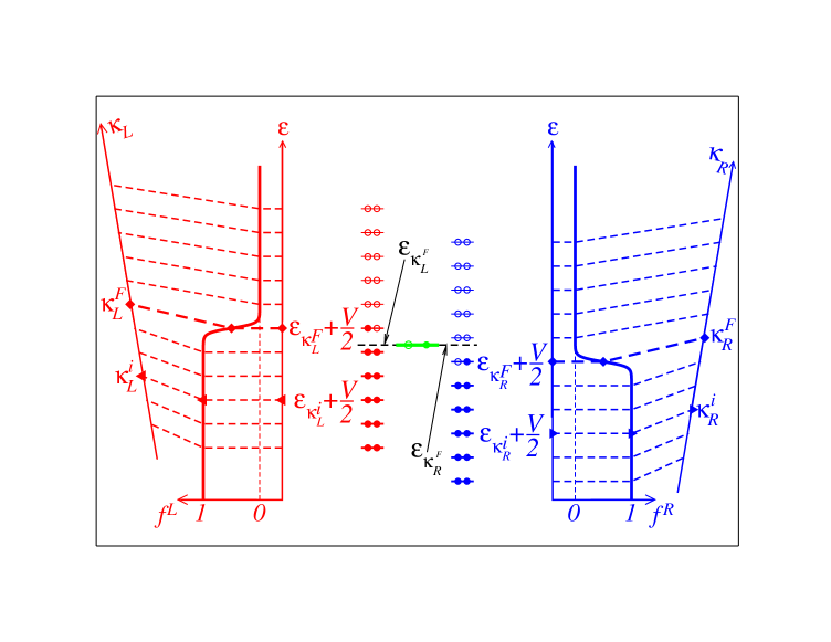
Figure 1: (Color online) Effect of an applied bias $V$ on the single-electron distributions $f^{L}$ and $f^{R}$ in the left ($L$) and right ($R$) electrodes. At $V=0$, the electrodes are in equilibrium, and their chemical potentials are equal, $\varepsilon_{{\kappa}_{L}^{F}}=\varepsilon_{{\kappa}_{R}^{F}}=\mu$ (black dashed horizontal line). The bias $V$ creates an imbalance between the chemical potentials $\mu_{L}=\varepsilon_{{\kappa}_{L}^{F}}+V/2$ and $\mu_{R}=\varepsilon_{{\kappa}_{R}^{F}}-V/2$ responsible for the current flow. The figure visualizes the fact that the bias only shifts the single-electron energies $\varepsilon_{{\kappa}_{L,R}}$ in the two electrodes by $\pm V/2$ in opposite directions: $\varepsilon_{{\kappa}_{L}^{i}}(V)=\varepsilon_{{\kappa}_{L,R}^{i}}+V/2$ and $\varepsilon_{{\kappa}_{R}^{i}}(V)=\varepsilon_{{\kappa}_{R}^{i}}-V/2$. However, the bias affects neither the labels of the single-electron states [$\kappa_{L,R}^{i}(V)\equiv\kappa_{L,R}^{i}$] nor their occupancies: $f^{L,R}_{\kappa_{L,R}^{i}}(V)=f^{L,R}(\varepsilon_{{\kappa}_{L,R}^{i}}\pm V/2;V)=f^{L,R}(\varepsilon_{{\kappa}_{L,R}^{i}};V=0)=f^{L,R}_{\kappa_{L,R}^{i}}(V=0)$ [cf. Eq. (23)]. The representation in the figure is schematic: in reality, neither the energies $\varepsilon$ (vertical axes) nor the quantum indices $\kappa_{L,R}$ (oblique axes) have equidistant values.

By choosing now the electron occupancies to express the boundary conditions ($Q_{\kappa}\equiv\alpha_{\kappa}^{\dagger}\alpha_{\kappa}$) and assuming, as usual, that the electron distributions in the reservoirs are not affected by the coupling to the device, we can reexpress Eqs. (4) as

$$\left\langle\Psi\right|\alpha_{\kappa}^{\dagger}\alpha_{\kappa}\left|\Psi\right\rangle=\left\langle\Psi_{0}\right|\alpha_{\kappa}^{\dagger}\alpha_{\kappa}\left|\Psi_{0}\right\rangle,$$ (23)

which apply both to the left and the right electrodes. Most importantly, the quantities $Q_{\kappa,n}=\mathcal{X}_{\kappa,n}=\left\langle\Psi_{n}\right|\alpha_{\kappa}^{\dagger}\alpha_{\kappa}\left|\Psi_{0}\right\rangle$ entering the l.h.s. of Eq. (12) are real. With this choice, $\mathcal{Y}_{\kappa,n}\equiv 0$, and Eqs. (LABEL:eq-lambda) and (19) become two sets of decoupled equations for $\lambda$’s and $\chi$’s, respectively

$$\sum_{\kappa^{\prime}}\lambda_{\kappa^{\prime}}\sum_{n\neq 0}\frac{\mathcal{X}_{\kappa^{\prime},n}\mathcal{X}_{\kappa,n}}{E_{n}-E_{0}}=\sum_{n\neq 0}\frac{\mathcal{W}_{n}}{E_{n}-E_{0}}\mathcal{J}_{q,n},$$ (24)

$$\sum_{q^{\prime}}\chi_{q^{\prime}}\sum_{n\neq 0}\frac{\mathcal{J}_{q^{\prime},n}\mathcal{J}_{q,n}}{E_{n}-E_{0}}=0.$$ (25)

From the latter equations we get $\chi_{q}=0$,non and then Eq. (20) yields

$$J=0.$$ (26)

This means that the approach considered above predicts a vanishing zero-bias conductance ($G=J/V=0$) at least for the rather general models of the type (6). One should note that this prediction also holds if not all $\kappa$’s, but only some of the occupancies of the single-electron states are subject to constraints of the type (23). Furthermore, the prediction (26) also applies to the case where the constraints (9) are not applied for all the sites $q$, but, e. g., only at the two contacts (i. e., the current flowing from the left electrode into the device is equal to that from the device into the right electrode).

Needless to say, the prediction (26) of a vanishing current in the linear response limit (vanishing zero-bias conductance) is completely unphysical and flagrantly contradicts numerous well established results. The existence of a nonvanishing zero-bias conductance $G=G_{0}\equiv 2e^{2}/h$ in the textbook example of conduction through a resonant single level system,Datta (2005) or the fact that the same value $G_{0}$ characterizes the Kondo plateau in the transport through a single-electron transistor Izumida et al. (2001); Costi (2001) are only two particular cases, which are described by the general model (6) for which the above considerations apply.

Concerning the linear response limit of the variational approach discussed here, we still have the following comments. Without imposing any boundary conditions of the type (4), the minimization of $\mathcal{E}$ of Eq. (1) yields equations identical to Eqs. (15) and (19) if we set $\lambda_{\kappa}\equiv 0$. Because in this case the latter group of equations only possess the trivial solution $\chi_{q}=0$, the expansion coefficients obtained from Eq. (15) have the form $A_{n}=\mathcal{A}_{n}\equiv\mathcal{W}_{n}/(E_{0}-E_{n})$, i. e., the solution $|\Psi\rangle$ of Eq. (10) is nothing but the ground state $|\mathcal{G}\rangle$ of the total Hamiltonian $H+W$ obtained within the first-order perturbation theory with respect to $W$. Being the ground state, that is, an eigenstate of the total Hamiltonian, it obviously obeys the equation of continuity: the current is site independent, more precisely $J=J_{q}=\langle\mathcal{G}|j_{q}|\mathcal{G}\rangle=0$.bey When the supplementary (boundary) conditions (4) are imposed, the corresponding Lagrange multipliers become nonvanishing $\lambda_{\kappa}\neq 0$, as seen from Eq. (LABEL:eq-lambda) or even from the more particular Eq. (LABEL:eq-lambda-nu). Consequently, $A_{n}\neq\mathcal{A}_{n}$, that is, the solution of optimization does differ from the ground state with applied bias, $|\Psi\rangle\neq|\mathcal{G}\rangle$. The essential point is that, as we have seen above, in order to sustain a nonvanishing current ($J\neq 0$), the matrix elements of the operators employed to impose the boundary conditions should have nonvanishing imaginary parts, $\mbox{Im\,}Q_{\kappa,n}\equiv\mathcal{Y}_{\kappa,n}\neq 0$. Luckily, this happens to be the case if the Fano operator (5) is used in Eq. (4), which amounts to formulate the boundary conditions in terms of the Wigner function.Bâldea and Köppel (2008) This choice yields nonvanishing currents, which sometimes, by chance, could be comparable with measured values Delaney and Greer (2004a, b) or look plausible.Fagas et al. (2006); Fagas and Greer (2007) However, as we have recently unambiguously demonstrated,Bâldea and Köppel (2008) the variational approach based on the Wigner function fails to recover the simplest results both for uncorrelated and correlated nanosystems, where its predictions are completely unphysical.

V Discussion and conclusion

In Ref. Bâldea and Köppel, 2008, we demonstrated that the DG approach Delaney and Greer (2004a, b); Delaney and Greer (2006) fails to reproduce the simplest well established results for transport in nanosystems and especially criticized the boundary conditions. In view of the fact that a reliable method to deal with correlated electron transport is hardly needed, one might still think to be able to develop the valid approach based on the DG method but employing other boundary conditions. Therefore, in the present paper, we have inquired the validity of the DG variational approach by considering constraints other than those imposed to the Wigner function at the boundaries. We believe that this investigation is important for specialists in the field thinking to apply such a modified DG scheme: the implementation for realistic ab initio calculations is by no means an easy task, and this probably explains why no other group applied the DG method in spite of its claimed success.

In the first part we have examined the linear response approximation by considering general boundary conditions. Further, we have critically analyzed the claim of DG on the Fermi-Dirac single-electron distributions. Namely, they claimed Delaney and Greer (2004a, b); Delaney and Greer (2006) that electron Fermi distribution functions, which are ubiquitously employed in transport theories, cannot be used in correlated systems because the single-particle picture breaks down, and resorting to the Wigner function was proposed as a way out of this difficulty. In Sect.  IV, we have explained that strong electron correlations in devices do not preclude the usage of single-electron distributions to express boundary conditions. The reason is that they should be imposed in electrodes, and there electrons are (assumed to be) uncorrelated. In fact, constraining single-electron distributions to be of Fermi-Dirac type in electrodes is the common feature of the most transport theories employed for macroscopic, mesoscopic and nanoscopic scale, and of interest there is just the case of correlated systems.

Obvioulsy, it is possible to impose constraints on the single-electron distributions in uncorrelated systems. As an important point of our analysis, we have demonstrated that, in particular, even for such uncorrelated systems and these standard boundary conditions (a case beyond of all question) the variational approach predicts a vanishing zero-bias conductance, which represents a completely unphysical result. Although this very fact is sufficient to invalidate this variational approach, the conclusion of the present investigation applies to more much general situations where strong electron correlations are present. Such more general examples include (but are not limited to) the systems described by the model Hamiltonian (6).

In principle, any theoretical approach of transport is based on two main ingredients. (i) First, one has to determine a certain quantity, which characterizes the transport cluster. (ii) Second, one has to impose boundary conditions to link the cluster to electrodes. The first ingredient is e. g., the transmission coefficient, Green function(s), or transition probabilities in Ladauer, NEGF, or master equation approaches, respectively. While this first ingredient is different from one transport approach to another, the second is common for virtually all approaches: whether correlated or not, the cluster is linked to electrodes by employing Fermi distributions. Because none of these approaches yields results which are manifestly unphysical, one has to admit that the formulation of the boundary conditions in terms of Fermi distribution functions is legitimate, or at least does not lead to manifest absurdities. If these boundary conditions were wrong, all these widely employed approaches would also yield unphysical results, but this is not the case. In fact, it is hard to imagine a physical situation more typical for using single-particle Fermi distributions than to describe electrons in metals (electrodes).

The approach of Delaney and Greer also comprises these two aspects: (i) One minimizes the total energy $E$ of the finite cluster used for transport calculations in the presence of an applied voltage. The energy of this open system is computed as the average value of a Hermitian Hamiltonian, $E=\langle H+W\rangle$. (ii) This is a constrained minimization: specifically, boundary conditions are applied to the Wigner function.

In Ref. Bâldea and Köppel, 2008, we demonstrated that, in the form proposed in Ref. Delaney and Greer, 2004a, this approach yields unphysical results and especially criticized the boundary conditions adopted by Delaney and Greer in the context of their approach. In the present paper, we have lifted these specific constraints and replaced them with the widely used boundary conditions, expressed in terms of Fermi functions. The result obtained, a vanishingly zero-bias conductance, is again quite unphysical. So, even with these usual boundary conditions, formulated in terms of Fermi distributions in electrodes, in the way common to the most widely employed transport theories, the approach based on the DG-variational method fails to pass the minimal decisive test, which any approach of electric transport at nanoscale must satisfy; namely, to be at least able to correctly describe the conductance in the linear response (Kubo) approximation or even to reproduce well established results of the Landauer theory in the absence of correlations (see, for example, Ref. Baer and Neuhauser, 2003).

The main result of our study is that the DG-variational approach does not work even with modified boundary conditions. This implies that the DG-approach is invalid not (or not only) because of the boundary conditions. If the imposition of the boundary conditions in terms of Wigner function were the only wrong point, the variational approach would produce correct results with correct boundary conditions. Doubtless, the Fermi functions represent the correct boundaries for uncorrelated system, a fact which proves the failure of the DG approach for that case. If the DG variational approach is incorrect even for uncorrelated systems, it is inconceivable that it works for correlated systems. We are then necessarily led to the conclusion that the other ingredient (i) of the DG-variational approach, namely the minimization of the cluster’s total energy, computed as the average of a Hermitian Hamiltonian, is inappropriate.

So, the failure of the approach of Delaney and Greer cannot be solely assigned to the manner in which the boundary conditions are imposed. Constraining the Wigner function $f(q,p)$ at the boundaries can also produce valuable physical results for the steady state current, provided that $f(q,p)$ is determined from the Liouville equation for $\partial f/\partial t=0$ and the values $f(q_{L,R},p)$ at the boundaries determined by the Fermi functions in reservoirs. Frensley (1991) However, in that case, the fact that the investigated systems are open leads to a non-Hermitian Liouville operator, which yields time irreversibility and currents that saturate to values characterizing the steady state flow. The counterpart of this procedure would be to employ non-Hermitian Hamilton operators $\mathcal{H}\neq\mathcal{H}^{\dagger}$, amounting to consider imaginary self-energies resulting from electrode-device interactions. Datta (2005) Attempting to develop a variational approach for a finite open system (device) described by a non-Hermitian Hamiltonian, e. g., by minimizing $\left\langle\left(\mathcal{H}+W-E\right)\left(\mathcal{H}^{\dagger}+W-E\right)\right\rangle$ instead of Eq. (1), might be an interesting alternative to the existing approaches to correlated transport, but to our knowledge such a method is not available at present. Till then, one is forced to admit that the variational procedure attempting to obtain the steady state current through a finite open system described by a Hermitian Hamiltonian and a wave function that minimizes the total energy in the presence of a voltage bias with certain boundary conditions is unable to reproduce well established results, on which there is an incontestable agreement between experiments and other theoretical approaches.

References

- Heurich et al. (2002) J. Heurich, J. C. Cuevas, W. Wenzel, and G. Schön, Phys. Rev. Lett. 88, 256803 (2002).
- Nitzan and Ratner (2003) A. Nitzan and M. A. Ratner, Science 300, 1384 (2003).
- Stokbro et al. (2003) K. Stokbro, J. Taylor, M. Brandbyge, J.-L. Mozos, and P. Ordej n, Comp. Mat. Sci. 27, 151 (2003).
- Baksmaty et al. (2008) L. O. Baksmaty, C. Yannouleas, and U. Landman, Phys. Rev. Lett. 101, 136803 (2008).
- (5) See, for example, New J. Phys 9 (2007), especially the focus articles 111-125.
- Landauer (1970) R. Landauer, Phil. Mag. 21, 863 (1970).
- Büttiker et al. (1985) M. Büttiker, Y. Imry, R. Landauer, and S. Pinhas, Phys. Rev. B 31, 6207 (1985).
- Haug and Jauho (1996) H. Haug and A.-P. Jauho, Quantum Kinetics in Transport and Optics of Semiconductors, vol. 123 (Springer Series in Solid-State Sciences, Berlin, Heidelberg, New York, 1996).
- Datta (2005) S. Datta, Quantum Transport: Atom to Transistor (Cambridge Univ. Press, 2005).
- White and Feiguin (2004) S. R. White and A. E. Feiguin, Phys. Rev. Lett. 93, 076401 (2004).
- Daley et al. (2004) A. J. Daley, C. Kollath, U. Schollwöck, and G. Vidal, Journal of Statistical Mechanics: Theory and Experiment 2004, P04005 (2004).
- Feiguin and White (2005) A. E. Feiguin and S. R. White, Phys. Rev. B 72, 020404 (2005).
- Bulla et al. (2008) R. Bulla, T. A. Costi, and T. Pruschke, Rev. Mod. Phys. 80, 395 (2008).
- Taylor et al. (2001) J. Taylor, H. Guo, and J. Wang, Phys. Rev. B 63, 245407 (2001).
- Brandbyge et al. (2002) M. Brandbyge, J.-L. Mozos, P. Ordejón, J. Taylor, and K. Stokbro, Phys. Rev. B 65, 165401 (2002).
- Rocha et al. (2006) A. R. Rocha, V. M. García-Suárez, S. Bailey, C. Lambert, J. Ferrer, and S. Sanvito, Phys. Rev. B 73, 085414 (2006).
- Hettler et al. (2003) M. H. Hettler, W. Wenzel, M. R. Wegewijs, and H. Schoeller, Phys. Rev. Lett. 90, 076805 (2003).
- Muralidharan et al. (2006) B. Muralidharan, A. W. Ghosh, and S. Datta, Phys. Rev. B 73, 155410 (2006).
- Thygesen and Rubio (2007) K. S. Thygesen and A. Rubio, J. Chem. Phys. 126, 091101 (2007).
- Reed et al. (1997) M. A. Reed, C. Zhou, C. J. Muller, T. P. Burgin, and J. M. Tour, Science 278, 252 (1997).
- Xiao et al. (2004) X. Xiao, B. Xu, and N. Tao, Nano Letters 4, 267 (2004).
- Dadosh et al. (2005) T. Dadosh, Y. Gordin, R. Krahne, I. Khivrich, D. Mahalu, V. Frydman, J. Sperling, A. Yacoby, and I. Bar-Joseph, Nature 436, 677 (2005).
- Tsutsui et al. (2006) M. Tsutsui, Y. Teramae, S. Kurokawa, and A. Sakai, Appl. Phys. Lett. 89, 163111 (2006).
- Delaney and Greer (2004a) P. Delaney and J. C. Greer, Phys. Rev. Lett. 93, 036805 (2004a).
- Delaney and Greer (2004b) P. Delaney and J. C. Greer, Int. J. Quant. Chem. 100, 1163 (2004b).
- Delaney and Greer (2006) P. Delaney and J. C. Greer, Proc. Roy. Soc. A 462, 117 (2006).
- Fagas et al. (2006) G. Fagas, P. Delaney, and J. C. Greer, Phys. Rev. B 73, 241314(R) (2006).
- Fagas and Greer (2007) G. Fagas and J. C. Greer, Nanotechnology 18, 424010 (2007).
- Bâldea and Köppel (2008) I. Bâldea and H. Köppel, Phys. Rev. B 78, 115315 (2008).
- (30) Any operator can be decomposed in a Hermitian and an anti-Hermitian part, where and are Hermitian operators (, ). Because the complex conjugate of Eq. (4) must also be satisfied, and must satisfy similar conditions, and .
- Caroli et al. (1971) C. Caroli, R. Combescot, P. Nozières, and D. Saint-James, J. Phys. C: Solid State Physics 4, 916 (1971).
- (32) We checked by straightforward numerical calculations that these determinants do not vanish for the case of the point contact attached to long electrodes and for the single electron transistor connected to short electrodes.
- (33) In ab initio calculations like those of Refs. Delaney and Greer, 2004a, b; Delaney and Greer, 2006, the equation of continuity (9) has to be imposed not only for a cluster of certain size (), but also on a spatial grid containing a finite number of points , and should also be sufficiently large to ensure convergence.
- (34) For example, in a half-filled cluster, where the number of electrons is equal to the number of sites.
- Izumida et al. (2001) W. Izumida, O. Sakai, and S. Suzuki, J. Phys. Soc. Jpn. 70, 1045 (2001).
- Costi (2001) T. A. Costi, Phys. Rev. B 64, 241310(R) (2001).
- (37) In fact, it is easy to understand that this result is not limited to the linear response approximation: it is just the exact ground state of , which minimizes of Eq. (1). Being an eigenstate, there is no need to impose the equation of continuity. The latter is automatically satisfied in the state , , but this ground state cannot sustain a finite current, i. e., . One should remark in this context that the assumption that all the model parameters of the Hamiltonian are real (which allows to consider that all the eigenstates are real) excludes superconductivity: the average of the current operator of Eq. (8) vanishes for any real state.
- Baer and Neuhauser (2003) R. Baer and D. Neuhauser, Chem. Phys. Lett. 374, 459 (2003).
- Frensley (1991) W. R. Frensley, Rev. Mod. Phys. 63, 215 (1991).