Network Model-Assisted Inference from Respondent-Driven Sampling Data

Abstract

Respondent-Driven Sampling is a method to sample hard-to-reach human populations by link-tracing over their social networks. Beginning with a convenience sample, each person sampled is given a small number of uniquely identified coupons to distribute to other members of the target population, making them eligible for enrollment in the study. This can be an effective means to collect large diverse samples from many populations.

Inference from such data requires specialized techniques for two reasons. Unlike in standard sampling designs, the sampling process is both partially beyond the control of the researcher, and partially implicitly defined. Therefore, it is not generally possible to directly compute the sampling weights necessary for traditional design-based inference. Any likelihood-based inference requires the modeling of the complex sampling process often beginning with a convenience sample. We introduce a model-assisted approach, resulting in a design-based estimator leveraging a working model for the structure of the population over which sampling is conducted.

We demonstrate that the new estimator has improved performance compared to existing estimators and is able to adjust for the bias induced by the selection of the initial sample. We present sensitivity analyses for unknown population sizes and the misspecification of the working network model. We develop a bootstrap procedure to compute measures of uncertainty. We apply the method to the estimation of HIV prevalence in a population of injecting drug users (IDU) in the Ukraine, and show how it can be extended to include application-specific information.

Keywords: Hard-to-reach population sampling; Link-tracing; Network sampling; Social networks; Exponential-family random graph model

1 Introduction

There is much interest in estimating features of hard-to-reach human populations. Such populations are characterized by the lack of a serviceable population sampling frame. In some settings, the target population is well-connected by a network of social relations. Link-tracing sampling strategies such as snowball sampling (Goodman, 1961) and respondent-driven sampling (RDS) (Heckathorn, 1997) are often used to leverage those social relations to sample beyond the small subgroup available to researchers. In these settings, subsequent samples are identified and selected based on their social ties with other members of the target population. The statistical literature dealing with such strategies (Goodman, 1961; Frank, 1971; Thompson, 1990; Thompson and Frank, 2000), typically assumes an idealized setting in which the initial sample is assumed to be a probability sample from the target population. The applied literature on the other hand Trow (1957); Watters and Biernacki (1989), has traditionally recognized that this is impractical, and therefore treated link-tracing samples (typically referred to as snowball samples, despite Goodman’s probabilistic framing) as convenience samples for which probability-based inferential methods are unfounded.

The work of Heckathorn and colleagues (Heckathorn, 1997; Salganik and Heckathorn, 2004; Heckathorn, 2007; Volz and Heckathorn, 2008) around the RDS specialization of link-tracing sampling is innovative in reducing the number of links followed per respondent, such that many waves of sampling are fostered, decreasing the dependence of the final sample on the initial convenience sample. The second main innovation of the RDS paradigm is in the respondent-driven nature of the sampling process in which subsequent samples are selected by the passing of coupons by current sample members, thus reducing the confidentiality concerns often present in hard-to-reach marginalized populations. While this approach does reduce the dependence of the final sample on the initial sample, it is possible for substantial bias to remain based on the initial sample of seeds, as studied in simulations by Gile and Handcock (2010) and illustrated empirically by Johnston (2010). Current estimation methods (Heckathorn, 1997; Salganik and Heckathorn, 2004; Heckathorn, 2007; Volz and Heckathorn, 2008; Gile, 2011), however, do not correct for biases introduced by seed selection. A common feature of networked populations is that the social ties are often more likely to occur between people that have similar attributes than those who do not, a tendency called homophily by attributes (Lazarsfeld and Merton, 1954; Freeman, 1996; McPherson et al., 2001). In this paper we present a novel approach and inferential frame to correct for bias introduced by seed selection and for the effects of homophily. In particular, we treat the problem of estimation of the population proportion of a binary covariate in populations where there exists homophily on the covariate of interest, based on a branching link-tracing sample beginning with seeds selected with bias with respect to that covariate.

There is a varied formal statistical literature on inference from link-tracing network samples. All of this work, however, involves the assumption that the initial sample is a probability sample drawn from a well-defined sampling frame, and that subsequent sampling is adaptive, or dependent on population characteristics only through their observed portions (Thompson and Seber, 1996). In the design-based framework, these works consider cases where sampling probabilities are known for all units in the analysis (Goodman, 1961; Frank, 1971, 2005; Thompson, 1992, 2006). Inference is then made without reference to any superpopulation model. In the likelihood frame, the literature treats cases where the adaptive sampling process is amenable to the model, and therefore the modeling can be conducted without explicit treatment of the sampling process (Thompson and Frank, 2000; Handcock and Gile, 2010; Pattison et al., 2009). The traditional approach to RDS, originally due to Heckathorn (1997), represents an alternative to this paradigm. The assumption of the original probability sample is replaced by an assumption of sufficient waves of sampling to adequately reduce the dependence of the sample on the original sample.

In this paper, we concern ourselves with a case in which none of these approaches suffice. The sampling probabilities of the units are not known, making the traditional design-based approaches inadequate. The initial sample is not a probability sample, so the sample is not adaptive or amenable, and any likelihood inference must consider the sampling process as well as the population model. Such a joint modeling approach has been conducted in a few works (Frank and Snijders, 1994; Felix-Medina and Thompson, 2004; Felix-Medina and Monjardin, 2006), but each of these requires an initial probability sample from some frame to allow for modeling of the sampling process. And while in some cases, the waves of sampling may be sufficient to suitably reduce the dependence on the initial sample, this is often not the case (Gile and Handcock, 2010), and we are interested in the cases when this does not hold.

We begin in Section 2 by introducing respondent-driven sampling. In Section 3, we then present our Model-Assisted inferential approach. Section 4 presents a simulation study illustrating the removal of bias introduced by the initial convenience sample. Our application to HIV prevalence estimation among injecting drug users in the Ukraine can be found in Section 5, and Section 6 presents a discussion and concluding remarks.

2 Respondent-Driven Sampling

2.1 Notation

We assume the target population consists of $N$ people (nodes) with labels $1,\ldots,N.$ Let the $N$-vector ${\bf z}$, represent a binary nodal outcome variable of interest. We refer to this variable as “infection status”, such that

$${\bf z}_{i}=\left\{\begin{array}[]{rl}0&i\textrm{ not infected}\\ 1&i\textrm{ infected.}\end{array}\right.~{}~{}~{}i\in 1\ldots N$$

We assume the target population is connected by a network of mutual relations with $N\times{N}$ adjacency matrix ${\bf y}$:

$${\bf y}_{ij}={\bf y}_{ji}=\left\{\begin{array}[]{rl}1&i\textrm{ and }j\textrm{ connected}\\ 0&i\textrm{ and }j\textrm{ not connected,}\end{array}\right.$$

and that this network forms a single connected component. Denote by ${\bf d}_{i}=\sum_{j}{\bf y}_{ij}$ the nodal degree, or number of network ties or alters of node $i$. Let ${\bf d}=\{{\bf d}_{1},\ldots,{\bf d}_{N}\}.$ Denote by ${\bf x}_{i}=\sum_{j}{\bf z}_{j}{\bf y}_{ij}$ the number of network ties node $i$ shares with infected nodes, and let ${\bf x}=\{{\bf x}_{1},\ldots,{\bf x}_{N}\}.$

2.2 Sampling Procedure

We consider an RDS procedure of the following form:

1. An small initial sample is selected from the population members accessible to researchers, typically using a convenience mechanism. They are typically 3-12 in number. They are called the seeds and comprise wave $k=0$ of the sample.

2. Each member of wave $k$ is given a small number (typically 2-3) of uniquely identified coupons to distribute among their alters.

3. Coupon recipients returning their coupons to the study center are subsequently enrolled in the study. A person recruited in a prior wave can not be recruited again. The wave number of a respondent is one more than that of their recruiter.

4. Steps (1) and (2) are repeated until the desired sample size is attained.

This process has proved effective at recruiting large and diverse samples from many hard-to-reach populations (Abdul-Quader et al., 2006), and has been widely used. It has been heavily used in the monitoring of disease prevalence and risk behaviors among high-risk populations such as sex workers, men who have sex with men, and injecting drug users (Malekinejad et al., 2008), largely in the service of the reporting requirements of UNAIDS for all countries with concentrated HIV epidemics (UNAIDS, 2008). It is also used by the US Centers for Disease Control and Prevention in the behavioral monitoring of injecting drug users in 25 large US cities (Lansky et al., 2007), and has also been used in other populations such as unregulated workers (Bernhardt et al., 2006) and jazz musicians (Heckathorn and Jeffri, 2001).

We represent the full sampling mechanism by the random variables:

$${\bf S}^{k}_{i}=\left\{\begin{array}[]{rl}1&\textrm{ person\ }i\textrm{ is sampled in wave }k\\ 0&\textrm{ otherwise}\end{array}\right.~{}~{}~{}i\in 1\ldots N,k\in 0,\ldots.$$

$${\bf S}_{i}=\sum_{k=0}^{\infty}{{\bf S}^{k}_{i}}=\left\{\begin{array}[]{rl}1&\textrm{ person\ }i\textrm{ is sampled}\\ 0&\textrm{ person\ }i\textrm{ is not sampled}\end{array}\right.~{}~{}~{}i\in 1\ldots N,$$

and let ${\bf s}^{k}$ denote the observed sampling vector corresponding to the people sampled in wave $k$. Based on the sampling procedure, we exactly observe the elements of ${\bf z},{\bf d}$ and ${\bf x}$ corresponding to $i:{\bf s}_{i}=1$. A variant when ${\bf x}$ cannot be observed directly, as in the application in Section 5, substitutes an estimate of ${\bf x}$ based on observed referral patterns.

Further we assume each respondent distributes a number of coupons completely at random from among their alters, with the number determined by a common distribution.

2.3 Design-based Inferential Approach

We consider design-based estimators for the population mean $\mu=\frac{1}{N}\sum_{i=1}^{N}{{\bf z}_{i}}$. Because the sampling probabilities of the people selected through RDS are almost never explicitly known, we follow Volz and Heckathorn (2008), and Gile (2011) in constructing a model for the sampling process, and estimating sampling probabilities accordingly. We use a generalized Horvitz-Thompson estimator of the form:

$$\hat{\mu}=\frac{\sum_{i=1}^{N}\frac{{\bf S}_{i}{\bf z}_{i}}{\hat{\pi}_{i}}}{\sum_{i=1}^{N}\frac{{\bf S}_{i}}{\hat{\pi}_{i}}},$$ (1)

where estimated sampling probabilities $\hat{\pi}_{i}=\mathbb{E}({\bf S}_{i}|\mathscr{S})$ are computed under an approximation $\mathscr{S}$ to the true RDS sampling process. If the inclusion probabilities were known this estimator is referred to as the Häjek estimator (Lumley, 2010), and typically performs better than the corresponding Horvitz-Thompson estimator (Särndal et al., 1992). The estimators introduced by Volz and Heckathorn (2008) and Gile (2011) differ, and ours further differs, in their specification of the sampling process $\mathscr{S}$.

Most inference from RDS data approximates the sampling process as a with-replacement random walk on the space of graph nodes, with transitions along the edges or social relations. For the purpose of inference, sampling is treated as a Markov chain at equilibrium (Salganik and Heckathorn, 2004; Volz and Heckathorn, 2008). Such inference involves sampling weights proportional to the self-reported degrees which are the equilibrium sampling probabilities of the with-replacement random walk on a connected network. While this is a useful first approximation, it has several limitations. First, as highlighted in Gile (2011), this type of inference does not respect the without-replacement nature of the sampling process, which can lead to biased estimates. Gile (2011) presents an approach correcting for this feature by substituting a without-replacement successive sampling approximation to the sampling process. Neither this, nor earlier estimators, however, address the fundamental issue of bias induced by the selection of the initial sample. Such bias is illustrated in Gile and Handcock (2010), as well as in the current paper, and correction for it is a key contribution of the present paper.

As with these earlier approaches, the first requirement of our sampling model is that it account for the different sampling probabilities by nodal degree. Unlike these other approaches, we further require our approach to account for the bias introduced by the selection of seeds in the presence of network homophily in the underlying population. This requires consideration of features of the social network, ${\bf y}$, in particular the homophily of the relations.

We make no assumptions about the mechanism for selecting the initial sample and will condition on the seed characteristics throughout the analysis.

If the network ${\bf y}$ were fully known, we could use simulation to estimate the sampling probability $\hat{\pi}_{i,{\bf y}}=\mathbb{E}({\bf S}_{i}|\mathscr{S},{\bf y},{\bf s}^{0})$ of each node, conditional on the selection of seeds, ${\bf s}^{0}$. Explicitly, we would repeatedly simulate RDS under sampling model $\mathscr{S}$ starting from ${\bf s}^{0}$ each time and compute the $\hat{\pi}_{i,{\bf y}}$ as the proportion of simulated samples containing node $i.$ These could be used in (1) to form an estimator. Unfortunately, ${\bf y}$ is typically only partially known, and so we apply a model-assisted approach.

3 A Model-Assisted Approach

Our approach is an extension of the model-assisted design-based approaches presented in Särndal et al. (1992). Existing work in this area uses a working model form to construct estimators that are (approximately) design-unbiased, whether the model holds or not, and have smaller design variance if the model does hold. Our case is slightly different. The sampling process we consider is only locally defined, and originates at a sample with unknown distribution. We therefore cannot guarantee design-unbiasedness. In fact, we require reference to a model form to recover approximate design-unbiasedness, rather than to improve efficiency. This is because the impact of the seed characteristics on the subsequent sample is mediated by the structure of the underlying social network.

Our approach is to assume a working superpopulation model from which the network was drawn and use it to estimate sampling probabilities conditional on the selection of the initial sample.

3.1 Network Working Model

We consider models of exponential-family random graph model (ERGM) form (Frank and Strauss, 1986; Hunter and Handcock, 2006; Hunter et al., 2008), conditional on the set of nodal degrees and infection statuses, and including a single additional parameter representing homophily on ${\bf z}$. In particular:

$$P({\bf Y}={\bf y}|{\bf z},{\bf d},\eta)=\frac{\exp({\eta g({\bf y},{\bf z})})}{c(\eta|{\bf z},{\bf d})},$$ (2)

where $g({\bf y},{\bf z})=\sum_{i,j=1}^{N}{\bf y}_{ij}{\bf z}_{i}(1-{\bf z}_{j})$, and $c(\eta|{\bf z},{\bf d})=\sum_{{\bf u}\in\mathscr{Y}({\bf z},{\bf d})}\exp(\eta g({\bf u},{\bf z}))$, and the space $\mathscr{Y}({\bf z},{\bf d})$ consists of all binary undirected networks consistent with ${\bf d}$ and ${\bf z}$ (the dependence on ${\bf d}$ and ${\bf z}$ is suppressed below). Note that this model form, as well as the simulation procedure to follow, requires knowledge of the population size $N$.

Given this model form, we use the estimator (1) based on sampling weights assumed constant over equivalence classes by degree and infection status and estimated under the model:

$$\hat{\pi}_{i,\eta}=\mathbb{E}({\bf S}_{i}|\mathscr{S},{\bf z},{\bf d},\eta,{\bf s}^{0})=\sum_{{\bf y}\in\mathscr{Y}({\bf z},{\bf d})}\hat{\pi}_{i,{\bf y}}P({\bf Y}={\bf y}|{\bf z},{\bf d},\eta),$$

where $\hat{\pi}_{i,{\bf y}}=\mathbb{E}({\bf S}_{i}|\mathscr{S},{\bf y},{\bf s}^{0})$, as defined in Section 2.3. Note that to treat these equivalence classes, we condition on the equivalence classes of the seed nodes selected, rather than the unique identities of those nodes.

We also do not know the network working model parameter $\eta$, and therefore must estimate it from the available data. The estimator is then computed using sampling probabilities based on the estimated network working model given by $\hat{\eta}$:

$$\hat{\pi}_{i,\hat{\eta}}=\mathbb{E}({\bf S}_{i}|\mathscr{S},{\bf z},{\bf d},\hat{\eta},{\bf s}^{0})=\sum_{{\bf y}\in\mathscr{Y}({\bf z},{\bf d})}\pi_{i,{\bf y}}P({\bf Y}={\bf y}|{\bf z},{\bf d},\hat{\eta})$$ (3)

These are the estimated probabilities used in our proposed estimator. This requires fitting a network working model to data sampled through RDS, which we address in the next section.

3.2 Fitting the Network Working Model

Thompson and Frank (2000) and Handcock and Gile (2010) provide an approach to fitting models of form similar to (2) to data sampled through link-tracing samples. Unfortunately, these approaches require a sample that is amenable to the model in question. That is:

$$P({\bf S}|{\bf y},{\bf d},{\bf z})=P({\bf S}|{\bf y}_{obs},{\bf d}_{obs},{\bf z}_{obs}),$$ (4)

where $*_{obs}$ represents the observed part of $*$, and also that the sampling and model parameters are separable. This is equivalent to the conditions for ignorability according to Rubin (1976) and Little and Rubin (2002). Unfortunately, in the case of RDS, condition (4) is violated by the convenience sample of seeds, which may well depend on unobserved characteristics.

Therefore, we require a novel approach to model fitting. As ${\bf d}$ and ${\bf z}$ are unknown, we construct design-based estimators of them from estimates of the sampling probabilities $\hat{\pi}_{i}.$ Specifically, let $\mathbb{N}_{kl}$ be the number of nodes of degree $k$ and infection status $l$, $k\in\{1,\ldots,N-1\}$, $l\in\{0,1\}$ and $\mathbb{N}=\{\mathbb{N}_{kl}\}_{k=1;l=0}^{k=N-1;l=1}.$ We estimate $\mathbb{N}$ and $g({\bf y},{\bf z})$ by,

$${\tilde{\mathbb{N}}}_{kl} ={1\over{N}}\sum_{i=1}^{N}\frac{{\bf S}_{i}\mathbb{I}({{\bf d}_{i}=k,{\bf z}_{i}=l})}{\hat{\pi}_{i}}$$ (5)

$${\tilde{g}({\bf y},{\bf x})} =\sum_{i=1}^{N}\frac{{\bf S}_{i}\left({\bf x}_{i}(1-{\bf z}_{i})+({\bf d}_{i}-{\bf x}_{i}){\bf z}_{i}\right)}{2\hat{\pi}_{i}}$$ (6)

where $\mathbb{I}(*)$ is the indicator function on $*$, and $\hat{\pi}_{i}$ is assumed constant for all $i:{\bf d}_{i}=k,{\bf z}_{i}=l$. Note that this requires the observation of $\{{\bf x}_{i}:{\bf S}_{i}=1,i=1,\ldots,N\}$. We then estimate $\eta$ as the natural parameter corresponding to the mean value parameter ${\tilde{g}({\bf y},{\bf x})}$ with the joint degree and infection status sequence implied by ${\tilde{\mathbb{N}}}.$ Details of this computation are given in the Supplemental Materials.

3.3 Algorithm

Note that the value of the network working model parameter, required to estimate $\pi,$ in turn, depends on the value of $\pi$. We therefore apply an approach similar to self-consistency (Lee and Meng, 2007) to find a joint solution to (5) and (6), as well as to the equations:

$$\hat{\pi}_{i,\hat{\eta}}=\mathbb{E}\left({\bf S}_{i}|\mathscr{S},{\bf z},{\bf d},\hat{\eta}({\tilde{\mathbb{N}}},{\tilde{g}({\bf y},{\bf x})})\right)~{}~{}~{}~{}~{}~{}~{}~{}~{}~{}~{}~{}~{}~{}i=1,\ldots,N.$$ (7)

This approach iterates between estimating the network working model parameter given values for the sampling probabilities, and then estimating the sampling probabilities given the network working model parameter. Explicitly, it is:

• Estimate $\hat{\pi}_{\hat{\eta}}$ proportional to degree $d_{i}$.

• Iterate the following steps:

  • Compute design-based estimates of statistics ${\tilde{\mathbb{N}}}_{kl}$ and ${\tilde{g}({\bf y},{\bf x})}$ using $\hat{\pi}_{\hat{\eta}}$ in (5) and (6).

  • Determine the working ERGM parameter $\eta$ corresponding to ${\tilde{\mathbb{N}}}$ and ${\tilde{g}({\bf y},{\bf x})}$.

  • Simulate $M$ networks according to the working ERG model. Estimate $\hat{\pi}_{\hat{\eta}}$ by simulated RDS sampling from the resulting networks.

• Use the resulting estimated probabilities, $\hat{\pi}_{\hat{\eta}}$, to form the weighted estimator of the quantity of primary interest:

  $$\hat{\mu}_{MA}=\frac{\sum_{i=1}^{N}\frac{{\bf S}_{i}{\bf z}_{i}}{\hat{\pi}_{\hat{\eta}}}}{\sum_{i=1}^{N}\frac{{\bf S}_{i}}{\hat{\pi}_{\hat{\eta}}}}.$$ (8)

The iterative nature of this procedure is similar to that used for the successive sampling estimator of Gile (2011). This algorithm differs in the core process of estimating the inclusion probabilities. More details of this procedure are provided in the supplemental materials.

The simulation procedure implicit in this estimation algorithm lends itself to a realistic bootstrap approach to standard error estimation. We present such a bootstrap in the supplemental materials, along with a simulation study illustrating its performance under a variety of conditions.

4 Comparing the Model-Assisted to Existing Estimators: A Simulation Study

Gile and Handcock (2010) present an extensive simulation study of RDS based, where possible, on a set of realistic characteristics of data from the CDC pilot study of RDS (Abdul-Quader et al., 2006). For comparison purposes, our simulation study uses the same simulated populations as Gile (2011), along with extensions necessary for our sensitivity analyses.

4.1 Study Design

Our simulation study is designed around three levels of simulation:

• The generation of random networks according to specified network features

• The generation of simulated RDS samples from each network

• The estimation of infection prevalence from each set of simulated sample data.

We use variants of the network and sampling parameters to study the behavior of the proposed estimator. Descriptions and levels of these parameters are listed in Tables 1 and 2.

Table 1: Parameters of simulated networks. Default parameters given in boldface.

Parameter	Meaning	Values
Number of nodes		1000, 715
Prevalence	$\mu=\frac{1}{N}\sum_{i}{{\bf z}_{i}}$	0.20
Mean degree	$\bar{{\bf d}}=\frac{1}{N}\sum_{i=1}^{N}\mathbb{E}(d_{i})=\frac{1}{2}\sum_{i,j=1}^{N}\mathbb{E}(Y_{ij})$	7
Homophily	$R=\frac{\frac{2}{N^{1}(N^{1}-1)}\sum_{i,j}{\bf z}_{i}{\bf z}_{j}\mathbb{E}(y_{ij})}{\frac{1}{N^{1}N^{0}}\sum_{i,j}{\bf z}_{i}(1-{\bf z}_{j})\mathbb{E}(y_{ij})}$	5, 3, 1
	where $N^{0}=N(1-\mu),N^{1}=N\mu$
Activity	$w=\frac{\bar{d}^{1}}{\bar{d}^{0}}=\frac{\frac{1}{N^{1}}\sum_{i,j}{\bf z}_{i}\mathbb{E}(y_{ij})}{\frac{1}{N^{0}}\sum_{i,j}(1-{\bf z}_{i})\mathbb{E}(y_{ij})}$	1, 1.8
Ratio

To allow for comparability across simulation conditions, throughout our simulations, we maintain the same true recoverable prevalence, $\mu=0.20$, the same sample size $n=500$, and the same mean degree ${\bar{\bf d}}=7$. We consider variations on the population size (hence the sample fraction), the degree of clustering or homophily on infection status, and differential rates of tie formation by infection status (or activity ratio). The parameter levels considered are summarized in Table 1.

Under each set of network parameters, networks are simulated according to an ERGM with sufficient statistics:

$$g_{1}({\bf y}) =\sum_{i=1}^{N}\sum_{j<i}{\bf y}_{ij}{\bf z}_{i}{\bf z}_{j}$$

$$g_{2}({\bf y}) =\sum_{i=1}^{N}\sum_{j<i}{\bf y}_{ij}(1-{\bf z}_{i})(1-{\bf z}_{j})$$ (9)

$$g_{3}({\bf y}) =\sum_{i=1}^{N}\sum_{j=1}^{N}{\bf y}_{ij}{\bf z}_{i}(1-{\bf z}_{j}).$$

These three terms correspond to the unique cells of the $2\times 2$ mixing matrix on ${\bf z}$, and for a given number of nodes $N$ and prevalence $\mu$, are uniquely defined by $\bar{\bf d}$, $R$, and $w$. Note that this model is similar to (2), but not identical. While (2) conditions on the fixed degree of each node, this model allows for stochastic variability in degrees around mean value parameters given by (4.1).

From each simulated network, a single RDS sample is drawn according to parameters in Table 2. A fixed number $n^{0}$ of seed nodes are selected with probability proportional to degree (the best case for the earlier estimators), from either the full population or from the infected nodes only (to simulate extreme seed bias). The simulated process treats the case of two coupons distributed by each respondent completely at random among its previously un-sampled alters. Two coupons are chosen for simplicity, and because it represents the sampling process better than either 3 (equating to the return of all coupons in practice) or 1 (resulting in non-branching chains).

Table 2: Parameters of simulated RDS sampling. Default parameters given in boldface.

Parameter	Meaning	Values
Number of Seeds	$n^{0}=\sum_{i}{\bf S}_{i}^{0}$	10, 6, 20
Seed Selection	Sequentially with probability proportional	full population,
	to degree from either:	infected nodes
Branching	From each sampled node, up to $n_{cup}$	2
	previously unselected alters are selected
	completely at random for subsequent sampling.
	$n_{cup}$ are selected whenever available.
Sample Size	Sampling stops when $n$ nodes have been sampled.	500

For each simulation case, we simulate 1000 networks with one RDS sample from each, and we compare five estimators, as summarized in Table 3.

Table 3: Five estimators compared in the simulation study.

Abbreviation	Source	Estimator
Mean	Naive sample mean of ${\bf z}_{i}$	$\hat{\mu}$
SH	Salganik and Heckathorn (2004)	$\hat{\mu}_{SH}$
VH	Volz and Heckathorn (2008)	$\hat{\mu}_{\rm VH}$
SS	Gile (2011)	$\hat{\mu}_{SS}$
MA	Current paper	$\hat{\mu}_{MA}$

4.2 Primary Results

We begin by studying the performance of the proposed estimator in settings where previous estimators have been found to perform well. In the first part of Figure 1, there is a relatively small sample fraction (50%, $N=1000$), no homophily on infection status ($R=1$), the ratio of mean degrees by infection ($w$) is 1, and seeds are chosen from the full population, so there is no bias induced by seed selection. In this case, none of the estimators considered exhibit bias, and the naive sample mean exhibits the lowest variance, although the variability is similar across estimators.

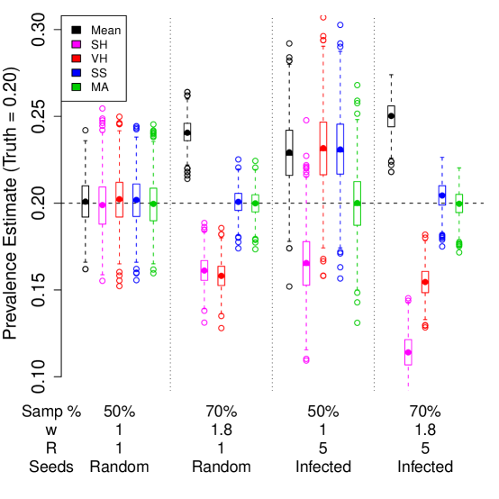
Figure 1: Comparison of performance of five RDS estimators under four conditions. $\hat{\mu}_{SS}$ and $\hat{\mu}_{MA}$ assume correct population size $N$. Results from 1000 simulations.

The second part of Figure 1 illustrates the case $\hat{\mu}_{SS}$ is designed to address. In this case, the sample fraction is large (about 70%, $N=715$), and infected nodes have mean degree 80% higher than that of uninfected ($w=1.8$). In this case there is still no homophily ($R=1$), and no seed bias. Here, the higher-degree infected nodes are over-represented in the sample, resulting in positive bias in the sample mean. Because of assumed linear mapping from degree to sampling probability, $\hat{\mu}_{SH}$ and $\hat{\mu}_{\rm VH}$ over-correct for this feature, resulting in negative bias. $\hat{\mu}_{SS}$ and $\hat{\mu}_{MA}$ appropriately adjust for the over-sampling of infected nodes, resulting in unbiased estimators without increased variance.

The third section of Figure 1 considers the case the new estimator, $\hat{\mu}_{MA},$ is designed to address. There is homophily ($R=5$), and all seeds are selected from among the infected nodes. This case treats a smaller sample fraction ($N=1000$) and activity ratio 1 ($w=1$). Here, all of the earlier estimators exhibit bias due to the selection of seeds (note the direction of bias is different for $\hat{\mu}_{SH}$), while the proposed estimator appropriately corrects for the selection of seeds.

The final case considers the joint effects of large sample fraction ($N=715$), non-activity ratio ($w=1.8$), homophily ($R=5$), and biased selection of seeds (all infected). Here, the sample mean over-represents the higher-degree and initially sampled infected nodes. $\hat{\mu}_{\rm VH}$ exhibits a strong negative bias, similar to that in the second case. The two effects jointly cause tremendous bias in $\hat{\mu}_{SH}$. $\hat{\mu}_{SS}$ is affected by seed bias, although not by the sample fraction. Here, again, the proposed estimator correctly adjusts for all of these effects. Although in this example the effects of sample fraction/activity ratio are of larger magnitude than those of seed bias/homophily, in practice the relative magnitudes of these will vary across data sets.

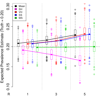
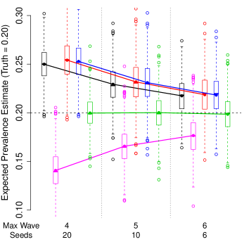
Figure 2: Comparison of the performance of five RDS estimators with biased seed selection and various levels of homophily and numbers of sampling waves. All treat $N=1000,w=1$, and all seeds are selected from among infected nodes only. The first subfigure illustrates the exacerbating effect of homophily on seed bias. The second illustrates the ameliorating effect of increased sampling waves on seed bias.

Figures 2 and 2 illustrate additional features important to the impact of seed selection on the bias of the sample mean and earlier estimators. In particular, Figure 2 illustrates that the bias is exacerbated by increased homophily in the underlying population, and Figure 2 illustrates that bias is attenuated by having more sampling waves (attained by selecting fewer seeds for fixed sample size and branching). In each of these cases, the proposed estimator has negligible bias. Note that for very high levels of homophily ($R=13$), the proposed estimator was found to exhibit positive bias, but of much smaller magnitude than that of the other estimators.

4.3 Sensitivity to the Population Size Estimate

In practice, the size of the hidden population, $N$, may not be known. We therefore conduct a sensitivity analysis illustrating the performance of the proposed estimator in the case of an inaccurate estimate $\hat{N}$ of $N$. We consider cases of $N-\frac{1}{2}(N-n)=\hat{N}_{s}<N$ and $N+\frac{1}{2}(N-n)=\hat{N}_{l}>N$. For each treatment of $\hat{N}$, we treat the four cases in Figure 1. $\hat{\mu}$ and $\hat{\mu}_{\rm VH}$ correspond to the extreme cases of $\hat{N}=n$ and $\hat{N}=\infty,$ respectively, so are plotted for reference alongside $\hat{\mu}_{SS}$ and $\hat{\mu}_{MA}$ for each level of $\hat{N}$.

Figures 3(a) and 3(c) illustrate that in the case of unity activity ratio and a smaller sample fraction, the assumed population size has little impact on the resulting estimators (note that in the case with $\hat{N}=715$ in Figure 3(c), seed bias leads to the perception of a non-unity activity ratio which, along with a smaller assumed population size results in the perception of a larger sample fraction).

Figures 3(b) and 3(d) illustrate that in the case of large sample fraction and activity ratio ($w\neq 1$), the assumed sample fraction does impact the estimators $\hat{\mu}_{SS}$ and $\hat{\mu}_{MA}$. When there is no seed bias (Figure 3(b)), these estimators perform nearly identically. Gile (2011) argues that in this case, $\hat{\mu}_{SS}$ interpolates between the sample mean and $\hat{\mu}_{\rm VH}$, and that trend seems to hold for $\hat{\mu}_{MA}$ as well. In the case of seed bias (Figure 3(d)), however, $\hat{\mu}_{SS}$ and $\hat{\mu}_{MA}$ differ, in that $\hat{\mu}_{MA}$ corrects for the bias induced by the seed selection.

Finally, it is worth noting that for smaller sample fractions, such as in Figure 3(c), the bias induced by seed selection may be of far greater magnitude than the bias induced in $\hat{\mu}_{\rm VH}$ by finite population effects. For this reason, for smaller sample fractions, $\hat{\mu}_{MA}$ may be able to correct for the more important form of bias, without being greatly affected by uncertainty in the population size.

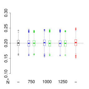
(a) None

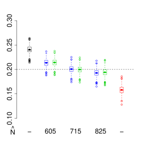
(b) Sample Fraction, Activity Ratio

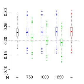
(c) Homophily, Seed Bias

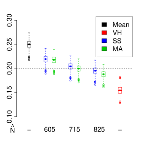
(d) All

Figure 3: Sensitivity of $\hat{\mu}_{SS}$ and $\hat{\mu}_{MA}$ to inaccurate population size under four network and sampling conditions. Gile (2011) argues that $\hat{\mu}_{SS}$ approaches the sample mean for small assumed population sizes, and approaches $\hat{\mu}_{\rm VH}$ for large assumed population sizes.

4.4 Sensitivity to the network working model

The role of the network working model is to provide a (stochastic) representation of the networked population. This model is the basis of the improved representation of the RDS design leveraged by the proposed estimator. The complexity of real-world social networks is high, so that simple network models will typically only capture a subset of this complexity.

The ERGM in (2) is designed to represent two levels of network structure that are important to model RDS. The first is the nodal level representation of the individual heterogeneity in the propensity to have social ties. This is via the nodal degrees which are also a measure of the centrality of the individuals in the network (Freeman, 1979). The second is at the dyadic level and captures the homophily, or propensity for ties to be between individuals with the same infection status (beyond that implied by the infection prevalence). As infection status is the primary outcome of interest, this homophily is the most important to capture. The model (2) does not capture third level triadic effects, those based on the structure of triads of relations between individuals. While these are tertiary to the monadic and dyadic effects they can influence the RDS. Unfortunately RDS results in branching tree patterns of observations that limit the empirical information on these triadic effects. Hence the model (2) presumes that the triadic effects are those that would be produced by the modeled monadic and dyadic components.

The purpose of this section is to assess the sensitivity of the estimator to this misspecification of the triadic effects. Explicitly, we will consider networked populations with higher levels of transitivity than specified in the network working model and compare the performance of the estimators. Transitivity is represented by the edgewise shared partner (alter) statistics, denoted ${\rm EP}_{0}({\bf y}),\ldots,{\rm EP}_{N-2}({\bf y})$, where ${\rm EP}_{k}({\bf y})$ is defined as the number of unordered pairs ${i,j}$ such that ${\bf y}_{ij}=1$ and $i$ and $j$ have exactly $k$ common alters. It is a measure of the shared friendliness of friends. The geometrically weighted edgewise shared partner (GWESP) statistic, conditional on the $\theta$ parameter, is

$$\textrm{gwesp}_{\theta}({\bf y})\equiv e^{\theta}\sum_{i=1}^{N-2}\left[1-(1-e^{-\theta})^{i}\right]{\rm EP}_{i}({\bf y})~{}~{}~{}~{}~{}~{}~{}~{}~{}~{}~{}~{}~{}\theta\geq 0.$$

The GWESP is an aggregate measure of local clustering or the overall “inwardness” of ties. The parameter $\theta$ controls just how “local” the clustering needs to be. If $\theta=0$ an edge with one shared partner counts the same as an edge with two or more shared partners. If $\theta>0$ an edge with one shared partner counts less than an edge with two or more shared partners. So large values of $\theta$ mean that very tight clustering is highly weighted and loose clustering is emphasized less. These terms have been developed for ERGM by Snijders et al. (2006) and Hunter and Handcock (2006).

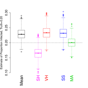
(a) Transitivity via GWESP with $\theta=0$.

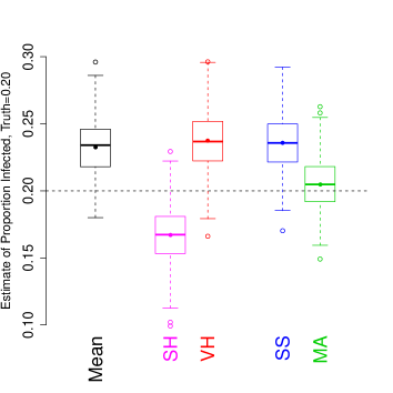
(b) Transitivity via GWESP with $\theta=1$.

Figure 4: Comparison of performance of five RDS estimators when the network working model misspecifies the transitivity. The populations in the left panel have ten times the GWESP with $\theta=0$ and the right panel with $\theta=1$. Results from 1000 simulations.

Most real-world networked populations over which RDS will be applied may be expected to have higher levels of transitivity than that produced by monadic and dyadic effects. Here we will consider two ways to produce networks with higher propensities for “friends of friends to be friends”. To investigate the relative performance of the estimator in populations with higher transitivity, we generate networks with exactly the same monadic and dyadic statistics as those considered in Section 4.2 but with higher transitivity as measured by the GWESP statistic. We do this by adding a $\textrm{gwesp}_{\theta}({\bf y})$ term to the model (4.1) and inflating the mean value parameter of the $\textrm{gwesp}_{\theta}({\bf y})$ while holding the mean value parameters of the other terms, as well as the degrees of each node, fixed. We then simulate networks from the resulting model, and apply the sampling and estimation procedures.

To test the correction for seed bias under model misspecification, we consider the populations in the third section of Figure 1. These have a smaller sample fraction ($N=1000$), high homophily ($R=5$), no differential activity ($w=1$) and biased selection of seeds (all infected). We take the same 1000 populations and re-generate them with the exactly the same degree sequences and homophily but with increased transitivity (as measured by the $\textrm{gwesp}_{\theta}({\bf y})$).

Figure 4 compares the same estimators as in Figure 1. The left panel consider populations with $\textrm{gwesp}_{0}({\bf y})$ ten times that in the original. A value of $\theta=0$ means that the statistic measures the number of pairs of people that are connected both by a direct edge and by a two-path through another person (that is, the number of edges minus the number of edges connected by no two-paths). As can be seen, the performance of $\hat{\mu}_{MA}$ is little effected by the increased transitivity. The right panel compares populations with ten times $\textrm{gwesp}_{1}(y).$ A value of $\theta=1$ means that the statistic weighs up the connectedness of edges with more weight on the terms with more shared partners. In this case $\hat{\mu}_{MA}$ has modest positive bias (0.46%) and similar variance compared to the estimators on the original populations.

5 Application to HIV prevalence in Hidden Populations

We apply our estimator to data collected in 2007 among injecting drug users (IDU) in Mykolaiv, Ukraine. The HIV epidemic in the Ukraine is one of the most severe in Europe, and still growing. As of 2009, the adult HIV prevalence was estimated at 0.86% (Ukrainian AIDS Centre, 2009). Ukraine’s epidemic is most severe among injecting drug users and their sexual partners, who account for the majority of new infections (United States Agency for International Development, 2010). The data we consider here were collected as part of a series of studies of IDU across major Ukrainian cities in 2007 (Kruglov et al., 2008). We focus on the data collected in Mykolaiv because, by chance and because of the contacts available to the researchers, all seeds in this sample were HIV positive.

This study began with 6 seeds and continued until wave 10, with 31 samples from wave 10, and a total of 260 samples. The average wave number was 6.1. The homophily based on HIV status for the population is estimated to be $R=2.47$ and the differential activity is estimated to be 0.72.

Although the size of the population was not known precisely, an estimated range of population sizes is available through scale-up and multiplier methods (Kruglov et al., 2008; UNAIDS/WHO, 2003). We chose a population size, $N=4000$, near the low end of this range. The variability of population size estimates is quite large, with a point estimate closer to 8000 in 2008 (Berleva et al., 2010)). We used sensitivity analysis to verify that population size 4000 is sufficiently large that our estimates are insensitive to increased population size.

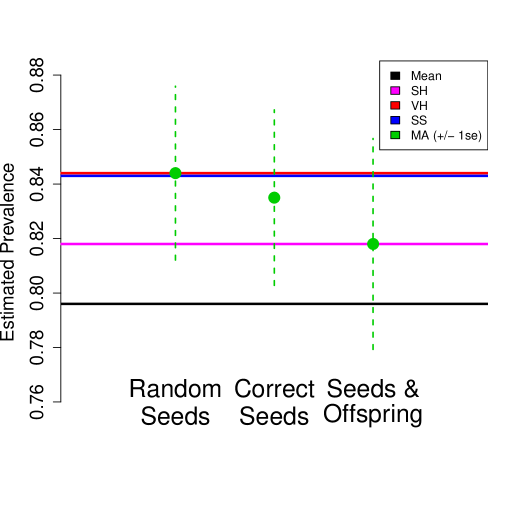
Figure 5: HIV prevalence estimates for injecting drug users in Mykolaiv, Ukraine, 2007.

We compare estimates for this application based on the current standard estimators ($\hat{\mu}_{SH}$, $\hat{\mu}_{\rm VH}$, $\hat{\mu}_{SS}$) and three variants of $\hat{\mu}_{MA}$, summarized in Figure 5. First, we consider a version of $\hat{\mu}_{MA}$ which does not correct for seed bias. In this case, we select the seeds of the simulated samples with probability proportional to degree and without regard to infection status. As illustrated in Figure 5, this results in an estimate very close to that given by $\hat{\mu}_{SS}$ and $\hat{\mu}_{\rm VH}$ ($\hat{\mu}_{\rm VH}=0.844$, $\hat{\mu}_{SS}=0.843$, $\hat{\mu}_{MA}=0.845$). In the second condition, we then apply the correction for seed bias, by matching the simulated seeds to the infection and degree characteristics of the observed seeds. This results in the second estimate in Figure 5, $\hat{\mu}_{MA}=0.837$. This adjustment is in the direction we would expect, decreasing the prevalence estimate, corresponding to down-weighting the group over-represented in the seeds. The modest magnitude of this adjustment can be attributed to the weak homophily in this network, relative to the number of sample waves, as well as the high prevalence, leading to a smaller difference between prevalence in the population and prevalence among the seeds than in our simulation study.

The third condition we considered highlights the flexibility and possibilities for extensions of $\hat{\mu}_{MA}$. We note that in these data, infection groups differed in their recruitment behavior. Some differences in recruitment behavior have been referred to as differential recruitment effectiveness in Heckathorn (2007), as well as in Tomas and Gile (2010) and Guntuboyina et al. (in preparation). This is a pattern in which one group systematically recruits more effectively than another group. In this case, however, the pattern was more complex. On average, infected and uninfected participants did not vary greatly in their recruitment effectiveness. However, uninfected participants in the early waves of the study recruited disproportionately few additional participants, as illustrated in Figure 6. Because of the branching nature of the sampling, this resulted in a dramatic under-representation of uninfected IDU in the survey. To correct for this, however, we needed to estimate and replicate offspring distributions varying by both infection status and survey wave.

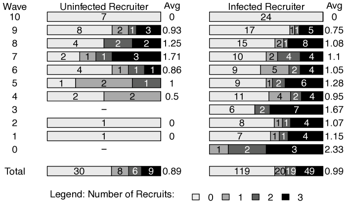
Figure 6: Distribution of number of successful recruitments by wave and infection status of recruiter. Uninfected recruiters were rare and unsuccessful in early waves, contributing to under-representation of uninfected participants in the sample. There were no uninfected participants in waves 0 (seeds) or 3.

We therefore applied a version of $\hat{\mu}_{MA}$, modified to reflect the empirical offspring distribution by wave and infection status. In most cases, this required simply assigning an offspring distribution equal to the empirical offspring distribution by wave and infection status. For uninfected recruiters in wave 3, we used averaged empirical values from waves 2 and 4. For waves 10 and beyond, we replicated the empirical results from wave 9. Whenever a simulated recruiter did not have enough eligible alters to allow for the number of recruits selected from the appropriate distribution, we assigned any unfulfilled recruitments to the next active recruiters of the same infection status with fewer than 3 assigned recruits. This is straight-forward to apply in our model-assisted setting and illustrates how this approach allows the approximation to the sampling design to be improved using available information.

The results of this analysis are illustrated in the third bar of Figure 5. The resulting estimate, $0.817$, was substantially lower than the earlier estimates, suggesting the offspring distribution had a substantial impact on the resulting estimates.

6 Discussion

In this article we introduce a new approach to estimation based on RDS data that uses a working model for the underlying networked population to more accurately estimate the inclusion probabilities necessary for design-based inference.

We demonstrate that this approach allows us to correct for differential sampling probabilities based on nodal degrees, as in earlier RDS estimators (Salganik and Heckathorn, 2004; Heckathorn, 2007; Volz and Heckathorn, 2008), as well as for finite population biases, as addressed by another earlier approach (Gile, 2011). In addition, our proposed estimator is able to adjust for the convenience sample of seeds, a feature not accounted for in any previous approaches.

We apply this approach to obtain improved estimation of HIV prevalence in an IDU population in the Ukraine. We improve the approximation to the actual RDS process resulting in improved estimates, and compute associated measures of uncertainty. We also show the flexibility of the working model approach. It allows for additional information available in a particular application to be incorporated via the ERGM framework, and leverages recent advances in that area (Handcock et al., 2008; Snijders et al., 2006). A significant weakness of our approach is the requirement that the population size is known. Our simulation study illustrates that the proposed estimator is indeed sensitive to estimates of population size, but as long as the population size is not greatly under-estimated, we do not expect it to perform worse than the earlier estimator $\hat{\mu}_{\rm VH}$, and in cases of bias induced by the sample of seeds, $\hat{\mu}_{MA}$ may perform substantially better than any existing estimator, even for highly inaccurate assumptions regarding the population size.

We therefore propose three practical regimes for the use of $\hat{\mu}_{MA}$. First, if the population size is known, the estimator may be applied directly. If the population size is unknown, but a range of estimates is available, the estimator may be applied across the range. If the results vary greatly, the uncertainty of the resulting estimator should be adjusted accordingly. Such may be the case, for example, in populations of men who have sex with men, who are assumed to constitute 1% - 3% of many populations. Finally, if no information on population size is available, $\hat{\mu}_{SS}$ may be compared with $\hat{\mu}_{\rm VH}$ to determine whether there are important finite population effects in this sample. If not, $\hat{\mu}_{MA}$ may then be applied to correct for any effects of seed bias. In the case where finite population effects are found, $\hat{\mu}_{MA}$ may be applied to diagnose the extent of seed bias at each of several estimates of population size. Note that in such cases, the earlier estimators also make an assumption about population size (i.e. that it is sufficiently large), and so do not avoid the problem of unknown population size.

Another important assumption is the form of the social network working model. Our estimator relies on a simple model, not because we believe it to be strictly accurate, but because we expect it to capture the network features most important to the sampling process, and because it is feasible to estimate from the available data. To assess the sensitivity of the estimator to the form of the working model we considered versions of populations with greatly increased transitivity, a feature not captured by the working model. The results indicate only modest impact of high transitivity on the estimator or it uncertainty. While this may not be universally true, it does indicate the ability of the working models to capture nodal and dyadic effects goes a long way to improve the representation of the RDS process.

Several extensions of this approach are possible. First, if data on the characteristics of all alters are not available, we may wish to estimate the sum of cross-group ties ($g({\bf y},{\bf x})$) based on referral patterns. Such an estimate is used in the application to HIV prevalence estimation (Section 5).

Our approach can also be extended to include additional measurable features of the network working model or sampling process, such as homophily on neighborhood of residence or bias in the passing of coupons. We illustrate one such extension in Section 5, in which we observe an aberrant pattern of recruitment by infection status, and adapt the estimator to condition on this pattern. Note that the resulting estimate is very close to that given by $\hat{\mu}_{SH}$. This is consistent with results in Tomas and Gile (2010) indicating that $\hat{\mu}_{SH}$ is not as susceptible to bias induced by differential recruitment effectiveness as $\hat{\mu}_{\rm VH}$ or $\hat{\mu}_{SS}$.

Further extensions of this approach will make it possible to consider the joint estimation of population size and prevalence, or correlations between multiple nodal variables. We explore these features in ongoing work.

We intend to make code available for these procedures in the R package RDS on CRAN (Handcock et al., 2009; R Development Core Team, 2007).

Inferential and Computation:

This supplement presents specifics of the estimation algorithms and our approach to standard error estimation (RDSMAsupplement.pdf)

References

- (1)
- Abdul-Quader et al. (2006) Abdul-Quader, A. S., Heckathorn, D. D., McKnight, C., Bramson, H., Nemeth, C., Sabin, K., Gallagher, K., and Jarlais, D. C. D. (2006), “Effectiveness of Respondent-Driven Sampling for Recruiting Drug Users in New York City: Findings from a Pilot Study,” Journal of Urban Health, 83, 459–476.
- Berleva et al. (2010) Berleva, G. O., Dumchev, K. V., Kobyshcha, Y. V., Paniotto, V. I., Petrenkon, T. V., Saliuk, T. O., and I. A. Shvab, I. A. (2010), Analytical Report based on sociological study results Estimation of the Size of Populations Most-at-Risk for HIV Infection in Ukraine in 2009,, Technical report, International HIV/AIDS Alliance in Ukraine.
- Bernhardt et al. (2006) Bernhardt, A., Heckathorn, D., Milkman, R., and Theodore, N. (2006), “Documenting Unregulated Work: A Survey of Workplace Violations in New York City,” The Future of Work, . http://www.unprotectedworkers.org
- Felix-Medina and Monjardin (2006) Felix-Medina, M. H., and Monjardin, P. E. (2006), “Combining link-tracing sampling and cluster sampling to estimate the size of hidden populations: A Bayesian-Assisted Approach,” Survey Methodology, 32, 187–195.
- Felix-Medina and Thompson (2004) Felix-Medina, M. H., and Thompson, S. K. (2004), “Combining link-tracing sampling and cluster sampling to estimate the size of hidden populations,” Journal of Official Statistics, 20, 19–38.
- Frank (1971) Frank, O. (1971), The Statistical Analysis of Networks, London: Chapman and Hall.
- Frank (2005) Frank, O. (2005), “Network Sampling and Model Fitting,” in Models and Methods in Social Network Analysis, eds. J. S. P. Carrington, and S. S. Wasserman, Cambridge: Cambridge University Press, pp. 31–56.
- Frank and Snijders (1994) Frank, O., and Snijders, T. A. B. (1994), “Estimating the size of hidden populations using snowball sampling,” Journal of Official Statistics, 10(1), 53–67.
- Frank and Strauss (1986) Frank, O., and Strauss, D. (1986), “Markov Graphs,” Journal of the American Statistical Association, 81(395), 832–842.
- Freeman (1979) Freeman, L. C. (1979), “Centrality in Social Networks: Conceptual Clarification,” Social Networks, 1(3), 223–258.
- Freeman (1996) Freeman, L. C. (1996), “Some antecedents of social network analysis,” Connections, 19, 39–42.
- Gile (2011) Gile, K. J. (2011), “Improved Inference for Respondent-Driven Sampling Data with Application to HIV Prevalence Estimation,” Journal of the American Statistical Association, 106, 135–146.
- Gile and Handcock (2010) Gile, K. J., and Handcock, M. S. (2010), “Respondent-Driven Sampling: An Assessment of Current Methodology,” Sociological Methodology, 40, 285–327. http://arxiv.org/abs/0904.1855v1
- Goodman (1961) Goodman, L. A. (1961), “Snowball Sampling,” Annals of Mathematical Statistics, 32, 148–170.
- Guntuboyina et al. (in preparation) Guntuboyina, A., Barbour, R., and Heimer, R. (in preparation), “Bootstrap-based population mean estimators for Respondent Driven Sampling,”.
- Handcock and Gile (2010) Handcock, M. S., and Gile, K. J. (2010), “Modeling Social Networks from Sampled Data,” Annals of Applied Statistics, 4(1), 5–25.
- Handcock et al. (2009) Handcock, M. S., Gile, K. J., and Neely, W. W. (2009), RDS: R Functions for Respondent-Driven Sampling, Hard-to-Reach Population Methods Research Group http://hpmrg.org/, Seattle, WA. R package version 0.10. http://CRAN.R-project.org/package=RDS
- Handcock et al. (2008) Handcock, M. S., Hunter, D. R., Butts, C. T., Goodreau, S. M., and Morris, M. (2008), “statnet: Software tools for the representation, visualization, analysis and simulation of social network data,” Journal of Statistical Software, 24(1). http://www.jstatsoft.org/v24/i01/
- Heckathorn (1997) Heckathorn, D. D. (1997), “Respondent-Driven Sampling: A New Approach to the Study of Hidden Populations,” Social Problems, 44, 174–199.
- Heckathorn (2007) Heckathorn, D. D. (2007), “Extensions of Respondent-Driven Sampling: Analyzing Continuous Variables and Controlling for Differential Recruitment,” Sociological Methodology, 37, 151–207.
- Heckathorn and Jeffri (2001) Heckathorn, D. D., and Jeffri, J. (2001), “Finding the beat: Using respondent-driven sampling to study jazz musicians,” Poetics, 28, 307–329.
- Hunter et al. (2008) Hunter, D. R., Goodreau, S. M., and Handcock, M. S. (2008), “Goodness of Fit for Social Network Models,” Journal of the American Statistical Association, 103, 248–258.
- Hunter and Handcock (2006) Hunter, D. R., and Handcock, M. S. (2006), “Inference in curved exponential family models for networks,” Journal of Computational and Graphical Statistics, 15(3), 565–583.
- Johnston (2010) Johnston, L. G. (2010), “Starting RDS Session III: Seeds,”. http://www.lisagjohnston.com/respondent-driven-sampling
- Kruglov et al. (2008) Kruglov, Y. V., Kobyshcha, Y. V., Salyuk, T., Varetska, O., Shakarishvili, A., and Saldanha, V. P. (2008), “The most severe HIV epidemic in Europe: Ukraine’s national HIV prevalence estimates for 2007,” Sexually Transmitted Infections, 84(Suppl 1), i37–41.
- Lansky et al. (2007) Lansky, A., Abdul-Quader, A. S., Cribbin, M., Hall, T., Finlayson, T. J., Garfein, R. S., Lin, L. S., and Sullivan, P. S. (2007), Developing an HIV behavioral surveillance system for injecting drug users: the National HIV Behavioral Surveillance System,, Technical Report Public Health Reports 2007; 122 Suppl 1: 48-55 17354527, Division of HIV/AIDS Prevention, National Center for HIV, STD, and TB Prevention, Centers for Disease Control and Prevention.
- Lazarsfeld and Merton (1954) Lazarsfeld, P., and Merton, R. (1954), “Friendship as social process: A substantive and methodological analysis,” in Freedom and Control in Modern Society, eds. M. Berger, T. Abel, and C. H. Page, New York: Van Nostrand, pp. 18–66.
- Lee and Meng (2007) Lee, T. C. M., and Meng, X.-L. (2007), “Self-Consistency: A General Recipe for Wavelet Estimation With Irregularly-spaced and/or Incomplete Data,”. ArXiv Preprint. http://arxiv.org/abs/math/0701196v1
- Little and Rubin (2002) Little, R. J. A., and Rubin, D. B. (2002), Statistical Analysis with Missing Data, 2nd. ed., Hoboken, New Jersey: John Wiley & Sons, Inc.
- Lumley (2010) Lumley, T. S. (2010), Complex Surveys: A Guide to Analysis Using R, New York: Wiley. Wiley Series in Survey Methodology.
- Malekinejad et al. (2008) Malekinejad, M., Johnston, L., Kendall, C., Kerr, L., Rifkin, M., and Rutherford, G. (2008), “Using Respondent-Driven Sampling Methodology for HIV Biological and Behavioral Surveillance in International Settings: A Systematic Review,” AIDS and Behavior, 12, 105–130.
- McPherson et al. (2001) McPherson, M., Smith-Lovin, L., and Cook, J. M. (2001), “Birds of a Feather: Homophily in Social Networks,” Annual Review of Sociology, 27, 415–444.
- Pattison et al. (2009) Pattison, P., Robins, G., Daraganova, G., Wang, P., Koskinen, J., and Snijders, T. (2009), “Modelling large social networks: statistical issues,”. Workshop Statistical Network Modeling, Nuffield College, Oxford.
- R Development Core Team (2007) R Development Core Team (2007), R: A Language and Environment for Statistical Computing, R Foundation for Statistical Computing, Vienna, Austria. ISBN 3-900051-07-0, Version 2.6.1. http://www.R-project.org/
- Rubin (1976) Rubin, D. B. (1976), “Inference and missing data,” Biometrika, 63, 581–592.
- Salganik and Heckathorn (2004) Salganik, M. J., and Heckathorn, D. D. (2004), “Sampling and Estimation in Hidden Populations Using Respondent-Driven Sampling,” Sociological Methodology, 34, 193–239.
- Särndal et al. (1992) Särndal, C.-E., Swensson, B., and Wretman, J. (1992), Model Assisted Survey Sampling, New York: Springer-Verlag.
- Snijders et al. (2006) Snijders, T. A. B., Pattison, P., Robins, G. L., and Handcock, M. S. (2006), “New Specifications for Exponential Random Graph Models,” Sociological Methodology, 36, 99–153.
- Thompson (1990) Thompson, S. K. (1990), “Adaptive Cluster Sampling,” Journal of the American Statistical Association, 85, 1050–1059.
- Thompson (1992) Thompson, S. K. (1992), Sampling, New York: Wiley.
- Thompson (2006) Thompson, S. K. (2006), “Adaptive web sampling,” Biometrics, 62(4), 1224–1234.