Implications of unitarity and analyticity for the $D\pi$ form factors

Abstract

We consider the vector and scalar form factors of the charm-changing current responsible for the semileptonic decay $D\rightarrow\pi l\nu$. Using as input dispersion relations and unitarity for the moments of suitable heavy-light correlators evaluated with Operator Product Expansions, including $O(\alpha_{s}^{2})$ terms in perturbative QCD, we constrain the shape parameters of the form factors and find exclusion regions for zeros on the real axis and in the complex plane. For the scalar form factor, a low energy theorem and phase information on the unitarity cut are also implemented to further constrain the shape parameters. We finally propose new analytic expressions for the $D\pi$ form factors, derive constraints on the relevant coefficients from unitarity and analyticity, and briefly discuss the usefulness of the new parametrizations for describing semileptonic data.

1 Introduction

The charm-changing current responsible for the semileptonic decay $D\rightarrow\pi l\nu$ is characterized by the vector and scalar form factors $f_{+}(t)$ and $f_{0}(t)$, defined by

$$\langle\pi^{-}(p^{\prime})|\overline{d}\gamma_{\mu}c|D^{0}(p)\rangle=(p^{\prime}+p)_{\mu}f_{+}(t)+(p-p^{\prime})_{\mu}f_{-}(t),$$ (1)

$$f_{0}(t)=f_{+}(t)+\frac{t}{M_{D}^{2}-M_{\pi}^{2}}f_{-}(t),\quad t=q^{2}=(p-p^{\prime})^{2}.$$ (2)

In the isospin limit the $D^{+}\to\pi^{0}$ form factors are obtained from $f_{\pm}(t)$ by multiplying with $1/\sqrt{2}$.

The knowledge of the shape of the $D\pi$ form factors in the physical region $M_{l}^{2}\leq t\leq(M_{D}-M_{\pi})^{2}$ is of interest for the determination of the element $|V_{cd}|$ of the Cabibbo-Kobayashi-Maskawa (CKM) matrix entering precision tests of the Standard Model. Recent measurements of the branching fractions of the semileptonic decays $D\rightarrow\pi l\nu$ and $D\rightarrow Kl\nu$ by the CLEO collaboration Ge:2008yi ; Besson:2009uv renewed the interest in the theoretical study of these processes.

Earlier studies on the heavy-light form factors are based on simple pole parametrizations which implement heavy quark scaling laws Becirevic:1999kt . The charm-changing form factors have been studied also in phenomenological models based on heavy quark and chiral symmetry Fajfer:2004mv , and more recently in the framework of Quantum Chromodynamics (QCD) light-cone sum rules (LCSR) Khodjamirian:2009ys . Lattice studies have been carried out for the $D\rightarrow\pi,K$ form factors in the whole physical region arXiv:0903.1664 ; Bailey:2010vz ; Na:2010uf ; DiVita:2011py . The $D\rightarrow\pi l\nu$ decay has also been considered recently in the emerging field of hard pion effective theory Bijnens:2010ws .

Analyticity and unitarity are useful tools for improving the knowledge on the form factors. The standard dispersion relations are of little use in the present case due to the scarce information on the $D\pi$ form factors on the unitarity cut. However, the method of unitarity bounds Okubo ; SiRa proves to be a useful approach in cases such as this. The method compensates for the lack of experimental information on the cut by an upper bound on the modulus squared of the form factor, obtained from unitarity and a dispersion relation for a suitable correlator of the same current, which can be evaluated by Operator Product Expansion (OPE) in the spacelike region. Employing standard mathematical techniques, one can then correlate the values of the form factor and its derivatives at different points inside the analyticity domain. Various versions of the method were applied to the pion electromagnetic form factor Caprini2000 ; Ananthanarayan:2008qj ; Ananthanarayan:2008mg ; Abbas:2009ye ; Anant:2011 , the $K\pi$ form factors MM ; AES ; BoMaRa ; BC ; Hill ; Abbas:2009uw ; Abbas:2009dz ; Abbas:2010jc ; Abbas:2010ns , as well as to the heavy-heavy RaTa ; deRafael:1993ib ; Boyd:1995sq ; Boyd:1995xq ; Boyd:1997kz ; CaLeNe and heavy-light form factors Boyd:1994tt ; Lellouch:1995yv ; BoCaLe . A review of the method was presented recently in Abbas:2010jc .

The $D\rightarrow\pi,K$ form factors were investigated with this method some time ago Boyd:1994tt . In this paper we revisit the problem, motivated in part by the progress in perturbative QCD calculations, which yield now the heavy-light correlators of interest to order $\alpha_{s}^{2}$ Chetyrkin:2001je . Since the correlators are given in Chetyrkin:2001je only for a massless light quark, we restrict our study to the $D\rightarrow\pi$ form factors.

In sect. 2 we briefly review the method of unitarity bounds in the heavy-light sector, extending previous studies by exploiting also higher moments of the corresponding correlation functions calculated in perturbative QCD Chetyrkin:2001je . The simultaneous use of several independent constraints is expected to increase the strength of the predictions. In sect. 2, we show also how to incorporate additional information on the form factors in the analyticity domain or on the unitarity cut. The numerical input of the method is reviewed in sect. 3.

In sect. 4 we investigate the model-independent constraints imposed by analyticity and unitarity on the low energy behaviour of the form factors. Specifically, we consider the shape parameters entering the Taylor expansion around $t=0$,

$$f_{k}(t)=f_{k}(0)\left(1+\lambda_{k}^{\prime}\frac{t}{M_{\pi}^{2}}+\frac{1}{2}\lambda_{k}^{\prime\prime}\frac{t^{2}}{M_{\pi}^{4}}+\cdots\right),~{}k=+,0,$$ (3)

and derive allowed ranges for the slopes $\lambda_{k}^{\prime}$ and the curvatures $\lambda_{k}^{\prime\prime}$. We work with dimensionless parameters, the choice of $M_{\pi}^{2}$ as normalization scale being merely a convention which does not influence the results (other choices, for instance $M_{D}^{2}$, would simply scale the coefficients by a constant factor). In the same section we further apply the same formalism in order to isolate regions on the real $t$-axis and in the complex $t$-plane where zeros of the form factors are excluded. The knowledge of the possible zeros is of interest, for instance, for the dispersive methods based on phase (Omnès-type representations) and for testing specific models of the form factors.

In sect. 5 we propose a new parametrization of the $D\pi$ form factors, which generalizes the systematic expansion proposed in BoCaLe for the $B\pi$ case by properly taking into account the position of the singularities generated by the first charm excited states. We derive constraints imposed by analyticity and unitarity on the coefficients of the parametrization and demonstrate its usefulness by fitting a sample of data points generated from the CLEO experimental results Ge:2008yi . Finally, in sect. 6 we summarize our conclusions.

2 Outline of the method

We start with the heavy-light invariant amplitudes $\Pi_{+}(q^{2})$ and $\Pi_{0}(q^{2})$ defined by the vector-vector correlation function

$$-(q^{2}g^{\mu\nu}-q^{\mu}q^{\nu})\Pi_{+}(q^{2})+q^{\mu}q^{\nu}\Pi_{0}(q^{2})\\ =i\int d^{4}xe^{iqx}\langle 0|TV^{\mu}(x)V^{\nu{\dagger}}(0)|0\rangle$$ (4)

where $V_{\mu}=\bar{d}\gamma_{\mu}c$. It is convenient to consider the moments of the invariant amplitudes at $q^{2}=0$,

$$\chi_{k}^{(n)}\equiv\frac{1}{n!}\frac{d^{n}}{(dq^{2})^{n}}\left[\Pi_{k}(q^{2})\right]_{q^{2}=0},\quad k=+,0,$$ (5)

which satisfy dispersion relations of the form

$$\chi_{k}^{(n)}=\frac{1}{\pi}\int_{t_{+}}^{\infty}\!dt\,\frac{{\rm Im}\Pi_{k}(t+i\epsilon)}{t^{n+1}},\quad k=+,0.$$ (6)

where $t_{\pm}=(M_{D}\pm M_{\pi})^{2}$.

From QCD it is known that the amplitude $\Pi_{+}(q^{2})$ satisfies a once subtracted dispersion relation, while for $\Pi_{0}(q^{2})$ an unsubtracted relation converges. Therefore, the quantities $\chi_{+}^{(n)}$ and $\chi_{0}^{(n)}$ are defined for $n\geq 1$ and $n\geq 0$, respectively.

The connection with the form factors $f_{+}(t)$ and $f_{0}(t)$ defined above is provided by unitarity: including in the unitarity sum for the spectral functions the contribution of the $D\pi$ states in the isospin limit leads to the inequalities

$${\rm Im}\Pi_{+}(t+i\epsilon)\geq\frac{3}{2}\frac{1}{48\pi}\displaystyle\frac{\left[(t-t_{+})(t-t_{-})\right]^{3/2}}{t^{3}}|f_{+}(t)|^{2},$$ (7)

$${\rm Im}\Pi_{0}(t+i\epsilon)\geq\frac{3}{2}\frac{t_{+}t_{-}}{16\pi}\frac{[(t-t_{+})(t-t_{-})]^{1/2}}{t^{3}}|f_{0}(t)|^{2},$$ (8)

which hold for $t>t_{+}$.

On the other hand, $\chi_{k}^{(n)}$ can be calculated in OPE as the sum of perturbative ($PT$) and nonperturbative ($NP$) contributions:

$$\chi_{k}^{(n)}=\chi_{k}^{(n)PT}+\chi_{k}^{(n)NP}.$$ (9)

The perturbative parts of the moments of heavy-light correlators for $n\leq 7$ were calculated up to two loops in Chetyrkin:2001je . Using these results we can write

$$\chi_{k}^{(n)PT}=c_{k,0}^{(n)}+c_{k,1}^{(n)}\,\alpha_{s}+c_{k,2}^{(n)}\,\alpha_{s}^{2},$$ (10)

where $\alpha_{s}$ is the strong coupling. The coefficients $c_{k,i}^{(n)}$ obtained using eqns. (34), (35) and the Appendix of Chetyrkin:2001je are compiled in Table 1 for several moments that will be used in this work.

The leading nonperturbative contribution of the quark and gluon condensates can be obtained from Lellouch:1995yv ; Generalis , and is written as

$$\chi_{+}^{(n)NP}=-\frac{1}{m_{c}^{2(n+2)}}\left[\bar{m}_{c}\langle\bar{u}u\rangle+\frac{\langle\alpha G^{2}\rangle}{12\pi}\right],$$ (11)

$$\chi_{0}^{(n)NP}=-\chi_{+}^{(n)NP}.$$ (12)

Table 1: Perturbative coefficients $c_{k,j}^{(n)}$ defined in (10) for the moments $\chi_{k}^{(n)}$ considered in the present work.

$i$	0	1	2
$c_{+,i}^{(1)}$	0.0024536	0.0027977	0.0066398
$c_{+,i}^{(2)}$	0.0001690	0.0002674	0.0009104
$c_{+,i}^{(3)}$	0.0000182	0.0000342	0.0001371
$c_{0,i}^{(0)}$	0.0126651	0.0095139	0.0045948
$c_{0,i}^{(1)}$	0.0008179	0.0013954	0.0037717
$c_{0,i}^{(2)}$	0.0000845	0.0001860	0.0006679

Table 2: Input values in the OPE calculation of the moments.

Quantity	Values
$m_{c}^{pole}$	$1.968\,{\rm GeV}$
$\overline{m}_{c}(\overline{m}_{c})$	$(1.27_{-0.09}^{+0.07})\,\rm GeV$
$\overline{m}_{c}(2\,{\rm GeV})$	$1.078\,{\rm GeV}$
$\langle\overline{u}u\rangle(2\,{\rm GeV})$	$((-0.254\pm 0.15)\,\rm GeV)^{3}$
$\langle\alpha G^{2}\rangle$	$(7.0\pm 1.3)\times 10^{-2}$
$\alpha_{s}(\overline{m}_{c})$	$0.39$

Table 3: OPE predictions for the vector correlators $\chi_{+}^{(n)}$.

$n$	$\chi_{+}^{(n)PT}$	$\chi_{+}^{(n)NP}$	$\chi_{+}^{(n)}$
1	0.0045547	0.0002723	0.0048270
2	0.0004118	0.0000704	0.0004821
3	0.0000524	0.0000182	0.0000706

Table 4: OPE predictions for the scalar correlators $\chi_{0}^{(n)}$.

$n$	$\chi_{0}^{(n)PT}$	$\chi_{0}^{(n)NP}$	$\chi_{0}^{(n)}$
0	0.0170744	-0.0010543	0.0160201
1	0.0019357	-0.0002723	0.0016634
2	0.0002586	-0.0000704	0.0001883

From the dispersion relations (6) and the unitarity conditions (7) and (8), it follows that each form factor $f_{k}(t)$ satisfies a set of integral inequalities written as

$$\frac{1}{\pi}\int^{\infty}_{t_{+}}dt\ \rho_{k}^{(n)}(t)|f_{k}(t)|^{2}\leq\chi_{k}^{(n)},\quad\quad k=+,0,$$ (13)

where the weights $\rho_{k}^{(n)}(t)$ are the product of $1/t^{n+1}$ with the phase space factors entering the unitarity relations. We use now the fact that the form factors $f_{+}(t)$ and $f_{0}(t)$ are analytic functions in the complex $t$-plane cut along the real axis from $t_{+}$ to $\infty$, and apply standard techniques to derive from eq.(13) constraints on their values, in particular on the shape parameters and on the regions in complex energy plane where zeros are excluded. First, the problem is brought to a canonical form by mapping the $t$-plane into the interior of a unit disk. This is achieved by the general conformal transformation

$$\tilde{z}(t,t_{0})=\frac{\sqrt{t_{+}-t_{0}}-\sqrt{t_{+}-t}}{\sqrt{t_{+}-t_{0}}+\sqrt{t_{+}-t}},$$ (14)

which maps the complex $t$-plane cut along the real axis for $t\geq t_{+}$ onto the unit disk $|z|<1$ in the complex plane $z\equiv\tilde{z}(t,t_{0})$, such that $\tilde{z}(t_{+},t_{0})=1$ and $\tilde{z}(\infty,t_{0})=-1$. The real parameter $t_{0}<t_{+}$ is arbitrary and denotes the point mapped onto the origin, $\tilde{z}(t_{0},t_{0})=0$. In the new variable, the inequality (13) takes the form

$$\frac{1}{2\pi}\int_{0}^{2\pi}{\rm d}\theta|g_{k}^{(n)}(e^{i\theta})|^{2}\leq\chi_{k}^{(n)},$$ (15)

where the analytic functions $g_{k}^{(n)}(z)$ are defined as

$$g_{k}^{(n)}(z)=f_{k}(\tilde{t}(z,t_{0}))\,w_{k}^{(n)}(z).$$ (16)

Here $\tilde{t}(z,t_{0})=t_{+}-(t_{+}-t_{0})(1-z)^{2}/(1+z)^{2}$ is the inverse of the function defined in (14) and $w_{k}^{(n)}(z)$ are outer functions, i.e. analytic and without zeros in $|z|<1$, such that their modulus squared on the boundary, $z={\rm e}^{i\theta}$, is equal to $\rho_{k}^{(n)}(\tilde{t}({\rm e}^{i\theta},t_{0}))$ multiplied by the Jacobian of the transformation (14). In our case the outer functions can be written in a compact form as

$$w_{+}^{(n)}(z)=\frac{1}{4\sqrt{2\pi}}[t_{+}-\tilde{t}(z,t_{0})](t_{+}-t_{0})^{-1/4}\\ \times\left[\sqrt{t_{+}-t_{-}}+\sqrt{t_{+}-\tilde{t}(z,t_{0})}\right]^{3/2}\\ \times\left[\sqrt{t_{+}-t_{0}}+\sqrt{t_{+}-\tilde{t}(z,t_{0})}\right]\\ \times\left[\sqrt{t_{+}}+\sqrt{t_{+}-\tilde{t}(z,t_{0})}\right]^{-(n+4)}$$ (17)

$$w_{0}^{(n)}(z)=\frac{\sqrt{3}(m_{D}^{2}-m_{\pi}^{2})\,w_{+}^{(n)}(z)}{\sqrt{t_{+}-\tilde{t}(z,t_{0})}[\sqrt{t_{+}-t_{-}}+\sqrt{t_{+}-\tilde{t}(z,t_{0})}]}.$$ (18)

In the notation we omitted for simplicity the dependence on $t_{0}$ of the functions $g_{k}^{(n)}(z)$, $w_{+}^{(n)}(z)$ and $w_{0}^{(n)}(z)$.

The analytic functions $g_{k}^{(n)}(z)$ admit the expansions

$$g_{k}^{(n)}(z)=g_{k,0}^{(n)}+g_{k,1}^{(n)}z+g_{k,2}^{(n)}z^{2}+\cdots$$ (19)

convergent in $|z|<1$. From eq.(15) it follows that the coefficients satisfy the inequality

$$\sum\limits_{j=0}^{\infty}(g_{k,j}^{(n)})^{2}\leq\chi_{k}^{(n)},\quad k=+,0.$$ (20)

Since each term in the left side is positive, the largest domain allowed for the first Taylor coefficients $g_{k,j}^{(n)}$, $0\leq j\leq J-1$ is obtained from (20) by setting the higher terms to zero. More generally, a rigorous correlation between these coefficients and the values $\xi_{k,p}^{(n)}\equiv g_{k}^{(n)}(z_{p})$ at some real points $z_{p}$, $1\leq p\leq P$, is given by the determinantal inequality Okubo ; SiRa ; BoMaRa ; Abbas:2010jc

$$\left|\begin{array}[]{c c c c c c}\bar{\chi}_{k}^{(n)}&\bar{\xi}_{k,1}^{(n)}&\bar{\xi}_{k,2}^{(n)}&\cdots&\bar{\xi}_{k,P}^{(n)}\\ \bar{\xi}_{k,1}^{(n)}&\displaystyle\frac{z^{2J}_{1}}{1-z^{2}_{1}}&\displaystyle\frac{(z_{1}z_{2})^{J}}{1-z_{1}z_{2}}&\cdots&\displaystyle\frac{(z_{1}z_{P})^{K}}{1-z_{1}z_{P}}\\ \bar{\xi}_{k,2}^{(n)}&\displaystyle\frac{(z_{1}z_{2})^{K}}{1-z_{1}z_{2}}&\displaystyle\frac{(z_{2})^{2J}}{1-z_{2}^{2}}&\cdots&\displaystyle\frac{(z_{2}z_{P})^{K}}{1-z_{2}z_{P}}\\ \vdots&\vdots&\vdots&\vdots&\vdots\\ \bar{\xi}_{k,P}^{(n)}&\displaystyle\frac{(z_{1}z_{P})^{J}}{1-z_{1}z_{P}}&\displaystyle\frac{(z_{2}z_{P})^{J}}{1-z_{2}z_{P}}&\cdots&\displaystyle\frac{z_{P}^{2J}}{1-z_{P}^{2}}\\ \end{array}\right|\geq 0.$$ (21)

where

$$\bar{\chi}_{k}^{(n)}=\chi_{k}^{(n)}-\sum_{j=0}^{J-1}(g_{k,j}^{(n)})^{2},$$ (22)

and

$$\bar{\xi}_{k,p}^{(n)}=\xi_{k,p}^{(n)}-\sum_{j=0}^{J-1}g_{k,j}^{(n)}z_{p}^{j},\quad p=1,2,...P.$$ (23)

The condition (21) is expressed in a straightforward way in terms of the values $f_{k}(t_{p})$ of the form factors at $t_{p}=\tilde{t}(z_{p},t_{0})$ and the derivatives at $t=0$, using eqns. (14) and (16). The generalization to complex points $z_{p}$ can be found in BoMaRa ; Abbas:2010jc .

In the present work we use the inequality (21) to obtain bounds on the slopes and curvatures of the form factors defined in eq.(3). As input we shall take the values $f_{+}(0)=f_{0}(0)$ at $t=0$, which are known from LCSR Khodjamirian:2009ys . An additional piece of information for the scalar form factor is provided by a low-energy soft-pion theorem of the Callan-Treiman CallanTreiman type, proved in DoKoSc , which in the $D\pi$ case reads

$$f_{0}(\Delta_{D\pi})=f_{D}/f_{\pi},$$ (24)

where $\Delta_{D\pi}=M_{D}^{2}-M_{\pi}^{2}$ is the relevant Callan-Treiman point and $f_{D}$ and $f_{\pi}$ are the meson decay constants.

As shown in Abbas:2010jc , from eq.(21) one can derive also regions where zeros of the form factors are excluded: this is done in a straightforward way by including in eq.(21) the input $f_{k}(z_{0})=0$ and finding the values $z_{0}$ for which the inequality is violated.

The constraints on the shape parameters can be further improved if some information on the form factors on the unitarity cut is available, in particular, if the phase $\delta_{k}(t)$ defined as

$$f_{k}(t+i\epsilon)=|f_{k}(t)|{\rm e}^{i\delta_{k}(t)},~{}~{}k=+,0,$$ (25)

is known along a low-energy interval, $t_{+}\leq t\leq t_{in}$. The implementation of this information can be done by the technique of generalized Lagrange multipliers and involves the solution of an integral equation, applied first to the $K\pi$ form factors in MM ; AES . A review of the method and more references are given in Abbas:2010jc .

Previous work on unitarity constraints for the heavy-light form factors Boyd:1994tt ; Lellouch:1995yv ; BoCaLe , exploited dispersion relations for the lowest moments of the correlators, corresponding to $n=1$ ($n=0$) for the vector (scalar) form factor. Here we use also the higher moments calculated to two loops in perturbative QCD Chetyrkin:2001je . Specifically, we use the dispersion relations for the moments $\chi_{+}^{(1)},\chi_{+}^{(2)},\chi_{+}^{(3)}$ and $\chi_{0}^{(0)},\chi_{0}^{(1)},\chi_{0}^{(2)}$. From the inequalities (15) we obtain, for each form factor, a family of three different constraints. The final allowed domain for the parameters of interest will be the intersection of the three individual domains.

Up to now we did not specify the parameter $t_{0}$ appearing in the conformal mapping (14). One can show that the bounds presented above are independent on $t_{0}$: indeed, the bounds are obtained by solving extremum problems upon the class of analytic admissible functions satisfying an $L^{2}$ norm condition like (15). Changing $t_{0}$ amounts to mapping a unit disk to another, and by this the class of admissible functions is not changed Duren . For deriving the bounds reported in sect. 4 we worked with $t_{0}=0$.

3 Choice of the input

We have presented in Table 1 the coefficients $c_{k,j}^{(n)}$ from Chetyrkin:2001je , entering the perturbative calculation of the moments $\chi_{k}^{(n)}$. In Table 2 we compile other quantities entering as input in the calculation of the moments. We exploited the approximate scale invariance of the product $m_{c}\langle\overline{u}u\rangle$ and evaluated it at a scale of 2 GeV. We took the masses and the strong coupling constant from the PDG tables PDG and used the renormalization group equations to evolve them to the relevant scale. The gluon condensate $\langle\alpha G^{2}\rangle$ has been taken from Narison:2010wb ; Narison:2011xe . The denominator of eq.(11) involves the pole mass Generalis . The $PT$ and $NP$ contributions and the total OPE predictions for $\chi_{+}^{(n)}$ and $\chi_{0}^{(n)}$ are summarised in Tables 3 and 4 for the values of $n$ specified above.

As mentioned earlier, we work in the isospin limit, taking for convenience for the $D$ meson the mass $M_{D}=1.869\,{\rm GeV}$ of the neutral $D$ meson, and for $\pi$ the mass $M_{\pi}=0.1395\,{\rm GeV}$ of the charged pion. Then $t_{+}=4.02\,{\rm GeV}^{2}$ and $t_{-}=2.98\,{\rm GeV}^{2}$.

In our analysis, we used as input the value $f_{+}(0)=0.67_{-0.07}^{+0.10}$ provided by LCSR Khodjamirian:2009ys , and $f_{0}(0)=f_{+}(0)$ as follows from eq.(2). Using $f_{D}=(206.7\pm 8.5\pm 2.5)\,{\rm MeV}$ and $f_{\pi}=(130.41\pm 0.03\pm 0.20)\,{\rm MeV}$ PDG , the low-energy theorem (24) gives $f_{0}(\Delta_{D\pi})=1.58\pm 0.07$ as quoted in Khodjamirian:2009ys .

In order to obtain the phase $\delta_{k}(t)$ defined by (25), a method useful in the case of the pion electromagnetic or the $K\pi$ weak form factors is to invoke Fermi-Watson theorem and take the precisely known phase shifts of the corresponding elastic partial waves. Since in the $D\pi$ case the elastic scattering is not yet investigated (except some comments on the $S$-wave in Bugg:2009tu ), we shall roughly estimate the phase of the form factors from the masses and widths of the resonances dominant at low energies. Namely, from the relativistic Breit-Wigner parametrization we obtain

$$\delta(t)=\arctan\left(\frac{M_{R}\Gamma(t)}{M_{R}^{2}-t}\right),$$ (26)

where $M_{R}$ is the mass and $\Gamma(t)$ the energy-dependent width

$$\Gamma(t)=\left(\frac{q(t)}{q(M_{R}^{2})}\right)^{2J+1}\frac{M_{R}}{\sqrt{t}}\,\Gamma_{R},$$ (27)

written in terms of the angular momentum $J$, the width $\Gamma_{R}$ and the c.m. momentum $q(t)=\sqrt{(t-t_{-})(t-t_{+})/4t}$.

The lowest vector $D^{*}$ and scalar $D_{0}^{*}$ excited states that couple to the $D\pi$ system produce singularities above the threshold, on the second Riemann sheet. The central values of the masses and widths of the lowest charged $D\pi$ vector and scalar resonances listed in PDG are: $M_{D^{*}}=2010.25\pm 0.14\,{\rm MeV}$, $\Gamma_{D^{*}}=96\pm 4\pm 22\,{\rm MeV}$ and $M_{D_{0}^{*}}=2403\pm 14\pm 35\,{\rm MeV}$, $\Gamma_{D_{0}^{*}}=283\pm 24\pm 34\,{\rm MeV}$.

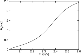
Figure 1: Phase of the $D\pi$ scalar form factor using a relativistic Breit-Wigner parametrization of the lowest resonance $D_{0}^{*}$.

We note that the vector resonance $D^{*}$ is very close to the threshold, so that a reasonable expression of the phase cannot be obtained from a Breit-Wigner parametrization, but in the scalar case we can assume that the phase $\delta_{0}(t)$ is reliably described by the expression (26) with $J=0$, which is plotted in Fig. 1. In our work we shall implement the phase up to the point $t_{in}=(2.6\,{\rm GeV})^{2}$, close to the first inelastic $D\eta$ channel opening at 2.42 GeV.

4 Constraints on the shape parameters and zeros

The interior of the ellipses shown in Fig.2 represent the allowed domains in the slope-curvature plane for the vector form factor, obtained with three moments $\chi^{(n)}_{+}$ of the vector correlator. We use the inequality (21) with no other input on the cut or in the analyticity domain except the value of $f_{+}(0)$ given above. The best (smallest) domain is given by the lowest moment, but the higher moments contribute to slightly reducing it, since one must take the intersection of all the domains in order to fulfill simultaneously the constraints. We also indicate the slope and curvature of the simple pole ansatz Becirevic:1999kt

$$f_{+}(t)=\frac{f_{+}(0)}{(1-t/M_{D^{*}}^{2})(1-\alpha_{D\pi}t/M_{D^{*}}^{2})},$$ (28)

with the parameters $\alpha_{D\pi}=0.21_{-0.07}^{+0.11}$ and $M_{D^{*}}=2.007\,{\rm GeV}$ proposed in Khodjamirian:2009ys . As seen from the figure, the point satisfies the unitarity constraints.

In the scalar case we use additional information on the phase and the soft pion theorem given by eq.(24). Fig. 3 illustrates the effect of these additional constraints, in the particular case of the bounds derived from the lowest moment $\chi_{0}^{(0)}$. We also show the slope and curvature from the pole ansatz Becirevic:1999kt

$$f_{0}(t)=\frac{f_{+}(0)}{1-t/(\beta_{D\pi}M_{D_{0}^{*}}^{2})},$$ (29)

with the parameters $\beta_{D\pi}=1.41\pm 0.06\pm 0.07$ and $M_{D_{0}^{*}}=2.318\,{\rm GeV}$ suggested in Khodjamirian:2009ys . The point satisfies the constraint imposed by the lowest moment, taking into account also the phase and the low-energy theorem (24).

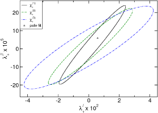
Figure 2: Constraints on the slope and curvature of the vector form factor obtained using as input different moments of the correlator. The point indicates the slope and curvature of the pole ansatz (28).

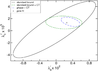
Figure 3: Constraints on the slope and curvature of the scalar form factor obtained with the moment $\chi_{0}^{(0)}$, from the standard bound and by including the phase and the low-energy theorem (24). The point indicates the slope and curvature of the pole ansatz (29).

In Fig. 4 we show the allowed domains obtained by using different moments $\chi_{0}^{(n)}$ of the scalar correlator. The phase and the low-energy constraint (24) have been included in all cases. Again, the smallest ellipse is obtained with the lowest moment $\chi_{0}^{(0)}$, but the simultaneous constraints reduce further this domain. We obtain rather small allowed regions in the slope-curvature plane when the phase as well as the low energy theorem are simultaneously taken into account. In particular, the point corresponding to the pole ansatz (29) falls outside the allowed regions imposed by the moments with $n=1$ and $n=2$.

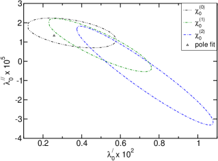
Figure 4: Constraints obtained by considering different moments of the scalar correlator, including information about the phase and the low-energy theorem (24). The point indicates the slope and curvature of the pole ansatz (29).

Figure 5: Domain without zeros for the vector form factor, obtained from the lowest moment $\chi_{+}^{(1)}$ and the input $f_{+}(0)$.

Figure 6: Domain without zeros for the scalar form factor, obtained from the lowest moment $\chi_{0}^{(0)}$ and the input $f_{0}(0)$ (smaller region) and using in addition the constraint (24) (larger region).

We mention that the above bounds were obtained with the central values of the input parameters. By varying simultaneouly all the input values we can obtain more conservative regions, which are slightly larger than the domains shown in the figures. The modification of the moments $\chi_{k}^{(n)}$ entering the inequalities (15) affects the results in a monotonous way: larger values of $\chi_{k}^{(n)}$ lead to weaker bounds. In our study we reduced this source of uncertainty by using more precise perturbative values of heavy-light current correlators, calculated in Chetyrkin:2001je at order $\alpha_{s}^{2}$. We have also studied the influence of the uncertainties in the resonance parameters for the mass and width of the scalar resonance PDG , and the uncertainty on the form factor values at $t=0$ and at the Callan-Treiman point (24). For instance, for the lowest moment illustrated in Fig. 3, the union of the ellipses resulting from the variation of $f_{+}(0)$, $f_{0}(\Delta_{D\pi})$, $M_{D^{*}}$ and $\Gamma_{D^{*}}$ within the errors quoted in sect. 3, and by enlarging $\chi_{+}^{(1)}$ by 10% yield the allowed ranges $0.08\cdot 10^{-2}\lesssim\lambda_{0}^{\prime}\lesssim 0.67\cdot 10^{-2}$ and $0.51\cdot 10^{-5}\lesssim\lambda_{0}^{\prime\prime}\lesssim 2.56\cdot 10^{-5}$, somewhat larger than ranges corresponding to the central values of the input, $0.12\cdot 10^{-2}\lesssim\lambda_{0}^{\prime}\lesssim 0.58\cdot 10^{-2}$ and $0.69\cdot 10^{-5}\lesssim\lambda_{0}^{\prime\prime}\lesssim 2.25\cdot 10^{-5}$.

A similar enlargement of the ellipses given by the next moments in Fig. 4 makes the pole ansatz compatible with the allowed domain given by $\chi_{1}^{(0)}$. It still remains outside the constraint yielded by $\chi_{2}^{(0)}$, but very close to the edge of the allowed domain.

As discussed in earlier works Abbas:2010ns ; Anant:2011 , the knowledge of the zeros is useful for specific fits and for testing general ideas about form factors. Although chiral symmetry for instance implies the existence of zeros in scattering amplitudes, there is not much information theoretically about them in the case of form factors. Nevertheless, phenomenological dispersive analyses often assume that zeros are absent in their fits to experimental data. Whereas remote zeros do not make any appreciable effect on these, nearby zeros if present will affect the behaviour of such fits and influence the number of subtractions. Therefore it is important to exclude zeros in the low-energy region.

For illustration, we consider in the following only the constraints imposed by the lowest moments, corresponding to $n=1$ in the vector case and $n=0$ in the scalar one, using as input the quoted value of $f_{+}(0)$ from LCSR. In the vector case we find that zeros on the real axis are excluded in the range $(-1.0,\,0.80)\,{\rm GeV}^{2}$. For the scalar case the range with no zeros is $(-2.51,\,1.55)\,{\rm GeV}^{2}$ for the standard bounds, while with the inclusion of the low-energy constraint (24) the range is increased to $(-3.55,\,3.89)\,{\rm GeV}^{2}$. In Figs. 5 and 6 we present the regions of excluded zeros in the complex $t$-plane for the vector and scalar form factors. In the scalar case the zeros are excluded in a larger domain if the low-energy constraint (24) is also imposed. In principle it would be possible to include also the phase and solve the integral equations for each point that is being tested. While an improvement of the size of the domains is expected, the computation is a laborious one and is beyond the scope of the present investigation.

5 New parametrization of the $D\pi$ form factors

Until recently, the most popular parametrization of the heavy-light form factors was the pole ansatz Becirevic:1999kt , given in eqs. (28) and (29) . A more general parametrization, based on a systematic expansion in powers of a conformal variable, was proposed in BoCaLe for the $B\pi$ vector form factor. In Khodjamirian:2009ys the same type of parametrization was adopted also in the $D\pi$ case. Specifically, the vector $D\pi$ form factor was written in Khodjamirian:2009ys as

$$f_{+}(t)=\frac{1}{1-t/M_{D^{*}}^{2}}\,\sum\limits_{j=0}^{J}b_{j}z^{j},$$ (30)

where $z=\tilde{z}(t,t_{0})$ is the variable defined in (14). However, this straightforward generalization is not entirely consistent, since the pole due to the lowest $D^{*}$ resonance is above the threshold on the second Riemann sheet, while in the expression (30) the singularity is on the real axis. Due to this fact, as we shall see, unitarity constraints on the free parameters $b_{j}$ cannot be derived. We mention that these constraints are useful not only for restricting the range of the independent parameters, but also for estimating the truncation error BoCaLe .

In the present work we write down improved parametrizations that take into account the proper position of the singularities produced by the first charm excited states. We propose for the vector form factor, instead of eq. (30), the representation

$$f_{+}(t)=\frac{M_{D^{*}}^{2}}{M_{D^{*}}^{2}-t+\sqrt{1-t/t_{+}}M_{D^{*}}\Gamma_{D^{*}}}\,\sum\limits_{j=0}^{J}b_{+,j}z^{j},$$ (31)

where as above $z=\tilde{z}(t,t_{0})$ is the conformal mapping (14). Similarly, for the scalar form factor, we write

$$f_{0}(t)=\frac{M_{D_{0}^{*}}^{2}}{M_{D_{0}^{*}}^{2}-t+\sqrt{1-t/t_{+}}M_{D_{0}^{*}}\Gamma_{D_{0}^{*}}}\,\sum\limits_{j=0}^{J}b_{0,j}z^{j}.$$ (32)

The coefficients $b_{k,j}$ are the parameters to be used in fits of data. Unitarity and analyticity imply that they are not completely free, but satisfy a constraint BoCaLe . In order to derive it, we insert the representations (31) and (32) into the definition (16) of the functions $g_{k}^{(n)}(z)$, extract the corresponding Taylor coefficients and apply the inequality (20). For simplicity, we consider only the constraints obtained with the lowest moments of the correlators. Then the above steps lead to the inequalities

$$\sum\limits_{i,j=0}^{J}B_{ij}^{(k)}b_{k,i}b_{k,j}\leq 1,\quad\quad k=+,0,$$ (33)

where $B_{ij}^{(k)}$ are calculated as BoCaLe .

$$B_{ij}^{(k)}=\frac{1}{\chi_{k}}\sum\limits_{m=0}^{\infty}\eta_{k,m}\eta_{k,m+|i-j|},\quad\quad k=+,0.$$ (34)

Here we used the notations $\chi_{+}\equiv\chi_{+}^{(1)}$, $\chi_{0}\equiv\chi_{0}^{(0)}$, and the numbers $\eta_{k,m}$ are the Taylor coefficients appearing in the expansions

$$\frac{M_{D^{*}}^{2}\,w_{+}^{(1)}(z)}{M_{D^{*}}^{2}-\tilde{t}(z,t_{0})+\sqrt{1-\tilde{t}(z,t_{0})/t_{+}}M_{D^{*}}\Gamma_{D^{*}}}=\sum\limits_{m=0}^{\infty}\eta_{+,m}z^{m},$$ (35)

$$\frac{M_{D_{0}^{*}}^{2}\,w_{0}^{(0)}(z)}{M_{D_{0}^{*}}^{2}-\tilde{t}(z,t_{0})+\sqrt{1-\tilde{t}(z,t_{0})/t_{+}}M_{D_{0}^{*}}\Gamma_{D_{0}^{*}}}=\sum\limits_{m=0}^{\infty}\eta_{0,m}z^{m},$$ (36)

where the outer functions $w_{k}^{(n)}(z)$ are defined in eqs. (17) and (18), and $\tilde{t}(z,t_{0})$ is the inverse of (14).

As remarked in sect. 2, the bounds derived in the previous section are independent of the choice of the parameter $t_{0}$ (in the calculations we have set $t_{0}$ to 0). By contrast, the parametrizations given above are based on truncated expansions and depend on $t_{0}$. For $t_{0}=0$ the semileptonic region $(0,t_{-})$ is mapped onto the range $(0,0.35)$ in the $z$-plane. This may lead to quite large truncation errors at the right end of the physical region. As suggested first in Boyd:1995xq ; Boyd:1994tt , it is more convenient to choose $t_{0}$ such as to map the physical range symmetrically around the origin of the $z$-plane, i.e. $\tilde{z}(0,t_{0})=-\tilde{z}(t_{-},t_{0})$. This gives the optimal value

$$t_{opt}\equiv(m_{D}+m_{\pi})(\sqrt{m_{D}}-\sqrt{m_{\pi}})^{2}=1.97\,\mbox{GeV}^{2},$$ (37)

when the physical range is mapped onto the segment (-0.17, 0.17) in the $z$-plane. In the following we shall investigate both choices $t_{0}=0$ and $t_{0}=t_{opt}$.

Since the outer functions and the BW representations are analytic in the unit disk and have no singularities on the boundary $|z|=1$ (the denominators vanish outside the unit disk), the expansions in the right hand sides of eqns.(35) and (36) are rapidly convergent. Therefore the quantities $B_{ij}^{(k)}$ can be calculated with precision by truncating the series in (34) at a finite order.

The numbers $B_{ij}^{(+)}$ and $B_{ij}^{(0)}$ up to $J=5$ for $t_{0}=0$ are

$$B_{00}^{(+)}=4.45\cdot 10^{-2},\quad B_{01}^{(+)}=2.53\cdot 10^{-2},$$

$$B_{02}^{(+)}=-4.53\cdot 10^{-4},\quad B_{03}^{(+)}=-3.60\cdot 10^{-3},$$

$$B_{04}^{(+)}=-4.60\cdot 10^{-5},\quad B_{05}^{(+)}=-5.81\cdot 10^{-4},$$ (38)

$$B_{00}^{(0)}=2.83,\quad B_{01}^{(0)}=1.18,\quad B_{02}^{(0)}=-1.68$$

$$B_{03}^{(0)}=-2.29,\quad B_{04}^{(0)}=-0.32,\quad B_{05}^{(0)}=1.60.$$ (39)

while for $t_{0}=t_{opt}$ the values read

$$B_{00}^{(+)}=4.45\cdot 10^{-2},\quad B_{01}^{(+)}=1.69\cdot 10^{-2},$$

$$B_{02}^{(+)}=-8.51\cdot 10^{-3},\quad B_{03}^{(+)}=-8.87\cdot 10^{-4},$$

$$B_{04}^{(+)}=5.75\cdot 10^{-4},\quad B_{05}^{(+)}=-3.10\cdot 10^{-3},$$ (40)

$$B_{00}^{(0)}=1.91,\quad B_{01}^{(0)}=0.25,\quad B_{02}^{(0)}=-1.61$$

$$B_{03}^{(0)}=-0.53,\quad B_{04}^{(0)}=1.09,\quad B_{05}^{(0)}=0.51.$$ (41)

Table 5: Sample of data on $f_{+}(t)$ used for a fit with the parametrization (31).

$n$	1	2	3	4	5	6	7	8	9	10
$t_{n}$	0	0.15	0.45	0.745	1.04	1.34	1.59	1.89	2.23	2.68
$f_{+}(t_{n})$	0.67	0.68	0.74	0.760	0.94	0.98	1.06	1.57	1.69	1.94
$\delta f_{+}(t_{n})$	0.10	0.03	0.04	0.05	0.05	0.06	0.08	0.11	0.23	0.29

The remaining coefficients are obtained from the relations $B_{i(i+j)}^{(k)}=B_{0j}^{(k)}$ and the symmetry property $B_{ij}^{(k)}=B_{ji}^{(k)}$ which follow from (34). In the calculation we used for the masses and widths of the resonances the central values from PDG , quoted above. The smaller values of $B_{ij}^{(+)}$ are due partly to the value of the QCD vector correlator and the form of the unitarity inequality (7), and partly to the parameters of the $D^{*}$-resonance.

Additional information, like the values of the form factors at $t=0$ and the low energy theorem (24) for the scalar form factor can be implemented easily. For the vector form factor it is useful to implement also the $P$-wave type behaviour at the unitarity threshold $t_{+}$. As discussed in BoCaLe , this condition is equivalent to

$$\left[\frac{{\rm d}f_{+}(\tilde{t}(z,t_{0}))}{{\rm d}z}\right]_{z=1}=0,$$ (42)

and amounts to the simple algebraic relation

$$M_{D^{*}}\Gamma_{D^{*}}\sum\limits_{j=0}^{J}b_{+,j}+2(M_{D^{*}}^{2}-t_{+})\sum\limits_{j=0}^{J}jb_{+,j}=0,$$ (43)

which must be fulfilled by the parameters $b_{+,j}$, simultaneously with the condition (33). These constraints are useful in the fits of the data, reducing the number of independent parameters.

Figure 7: Fit of a sample of data on the vector form factor $f_{+}(t)$ in the semileptonic region with the parametrization (31).

In order to illustrate the properties of the new parametrizations, we generated from the CLEO data Ge:2008yi a sample of values and errors for the vector form factor $f_{+}(t)$. We obtained the values from Table XIII of Ge:2008yi , using for convenience $|V_{cd}|=0.236$ as in Ge:2008yi . Assuming that the quoted values correspond to the center of the bins defined in Table IX of Ge:2008yi , and adding $f_{+}(0)$ from LCSR as quoted in sect. 3, we obtained the 10 data points given in Table 5. We then made a fit of these data using the expressions (31), with the threshold condition (43), using both $t_{0}=0$ and $t_{0}=t_{opt}$. The results of the two choices are actually very similar: with 2 independent parameters $b_{+,0}$ and $b_{+,1}$, the third one $b_{+,2}$ being determined from eq.(43), we obtained for $t_{0}=0$ a minimal $\chi^{2}=9.71$ with the optimal parameters:

$$b_{+,0}=0.665,\quad b_{+,1}=0.725,\quad b_{+,2}=-1.066,$$ (44)

while for $t_{0}=t_{opt}$ from (37) we obtained $\chi^{2}=9.67$ and the optimal coefficients

$$b_{+,0}=0.757,\quad b_{+,1}=0.397,\quad b_{+,2}=-0.852.$$ (45)

We have checked that the coefficients (44) and (45) satisfy the constraint (33) with $B_{jk}^{(+)}$ from (5) and (5), respectively. The above parametrizations lead actually to almost identical form factors in the semileptonic region, as shown in Fig. 7. However, the choice $t_{0}=t_{opt}$ allows a more accurate determination of the systematic error: assuming, as in BoCaLe , that a reasonable definition of the truncation error is given by $|b_{+,3}|_{max}|\tilde{z}(t,t_{0})|^{3}$, where $|b_{+,3}|_{max}$ is the maximum value of the next coefficient allowed by the condition (33) at the optimal point, we find for $t_{0}=0$, when $|b_{+,3}|_{max}=5.26$ and $\tilde{z}(t_{-},0)=0.35$, that this error reaches a value of about 7%, while for $t_{0}=t_{opt}$, when $|b_{+,3}|_{max}=4.28$ and $\tilde{z}(t_{-},t_{opt})=0.17$, the truncation error can be reduced to less than 1% in the whole semileptonic region.

The nontrivial role played by the condition (33) is seen if one makes a fit with one more independent parameter in (31). Then, for $t_{0}=t_{opt}$, the best fit without constraints gives $\chi^{2}=6.86$. However, the unitarity condition (33) is violated by the optimal parameters, and should be imposed explicitly for a suitable fit.

We finally remark that although the parametrization (31) for $t_{0}=t_{opt}$ is defined such as to optimize the description of the semileptonic region, it has a reasonable behaviour also outside this region and even on the unitarity cut. In particular, the polynomial in the numerator of (31) becomes complex for $t>t_{+}$, when $|z|=1$, but one can check that the phase of the product in (31) increases smoothly above the unitarity threshold and the resonance shape is not distorted, especially when the condition (43) is imposed.

The above exercise demonstrates the usefulness of the new parametrization (31) for data analysis. Of course, in a complete study the new expressions should be used directly in the fit of the partial branching fractions over bins in $t=q^{2}$, given in Ge:2008yi . The values provided by lattice calculations in the physical region arXiv:0903.1664 ; Bailey:2010vz ; DiVita:2011py can be also included in a combined fit, allowing a simultaneous determination of the vector form factor and of $|V_{cd}|$, as was done for the similar $B\pi$ case in BoCaLe .

6 Conclusions

In this work, we have explored the implications of analyticity and unitarity for the $D\pi$ form factors. The work was motivated by the recent experimental measurements of the semileptonic $D\to\pi l\nu$ decay Ge:2008yi ; Besson:2009uv of interest for the extraction of the element $|V_{cd}|$ of the CKM matrix. We have applied the formalism of unitarity bounds, which use as input the dispersion relations satisfied by the moments of suitable heavy-light correlators at $q^{2}=0$. The available calculations of the moments in perturbative QCD up to $O(\alpha_{s}^{2})$ terms Chetyrkin:2001je allow more precise predictions in this framework. We have derived a family of constraints to be satisfied by the shape parameters of both the scalar and vector form factors at $t=0$ and explored the region on the real axis and in the complex plane where the form factors cannot have zeros. The theoretical input at the Callan-Treiman point and the phase information for the scalar form factor play an important role in constraining the corresponding shape parameters. The exclusion regions for the zeros that we have isolated basically cover a significant part of the entire low energy region.

We have also proposed an improved parametrization of the $D\pi$ form factors in the semileptonic region, by properly implementing the singularities related to the lowest charmed resonances. The new parametrizations, given in eqns. (31) and (32) for the vector and scalar case, respectively, are based on truncated expansions in powers of the conformal mapping $z=\tilde{z}(t,t_{0})$ defined in (14), with coefficients satisfying the quadratic condition (33). Additional low-energy constraints or the threshold behaviour for the vector form factor can be easily implemented, as shown above. Using a sample of values produced from the CLEO experimental data Ge:2008yi , we demonstrated the usefulness of the new parametrization for the description of the semileptonic data and a reasonable estimate of the systematic error. A more complex analysis, allowing an accurate simultaneous prediction of the form factor and of $|V_{cd}|$, implies combined fits of the partial branching fractions over bins and of the LCSR and lattice predictions. This analysis will be reported in a future work.

Acknowledgements: BA thanks the Department of Science and Technology, Government of India, and the Homi Bhabha Fellowships Council for support. IC acknowledges support from CNCS in the Program Idei, Contract No. 464/2009 and from ANCS, Contract PN 09370102.

References

- (1) J.Y. Ge et al. [CLEO Collaboration], Phys. Rev. D 79, 052010 (2009) [arXiv:0810.3878 [hep-ex]].
- (2) D. Besson et al. [CLEO Collaboration], Phys. Rev. D 80, 032005 (2009) [arXiv:0906.2983 [hep-ex]].
- (3) D. Becirevic and A.B. Kaidalov, Phys. Lett. B 478, 417 (2000) [arXiv:hep-ph/9904490].
- (4) S. Fajfer, J.F. Kamenik, Phys. Rev. D 71, 014020 (2005) [hep-ph/0412140].
- (5) A. Khodjamirian, C. Klein, T. Mannel and N. Offen, Phys. Rev. D 80, 114005 (2009) [arXiv:0907.2842 [hep-ph]].
- (6) A. Al-Haydari et al. [QCDSF Collaboration], Eur. Phys. J. A 43, 107 (2010) [arXiv:0903.1664 [hep-lat]].
- (7) J.A. Bailey et al. [Fermilab Lattice and MILC Collaborations], PoS LATTICE2010, 306 (2010) [arXiv:1011.2423 [hep-lat]].
- (8) H. Na, C. T. H. Davies, E. Follana, G. P. Lepage and J. Shigemitsu, Phys. Rev. D 82, 114506 (2010) [arXiv:1008.4562 [hep-lat]].
- (9) S. Di Vita, B. Haas, V. Lubicz, F. Mescia, S. Simula, C.Tarantino for the ETM Collaboration, Published in PoS LAT2010:301. e-Print: arXiv:1104.0869 [hep-lat]
- (10) J. Bijnens and I. Jemos, Nucl. Phys. B 840, 54 (2010) [Erratum-ibid. B 844, 182 (2011)] [arXiv:1006.1197 [hep-ph]].
- (11) S. Okubo, Phys. Rev. D 3 (1971) 2807.
- (12) V. Singh and A.K. Raina, Fortsch. Phys. 27 (1979) 561.
- (13) I. Caprini, Eur. Phys. J. C 13, 471 (2000) [arXiv:hep-ph/9907227].
- (14) B. Ananthanarayan and S. Ramanan, Eur. Phys. J. C 54, 461 (2008) [arXiv:0801.2023 [hep-ph]].
- (15) B. Ananthanarayan and S. Ramanan, Eur. Phys. J. C 60, 73 (2009) [arXiv:0811.0482 [hep-ph]].
- (16) G. Abbas, B. Ananthanarayan and S. Ramanan, Eur. Phys. J. A 41, 93 (2009) [arXiv:0903.4297 [hep-ph]].
- (17) B. Ananthanarayan, I. Caprini, I.Sentitemsu Imsong, Phys. Rev. D83 096002 (2011) [arXiv:1102.3299 [hep-ph]]
- (18) M. Micu, Phys. Rev. D 7, 2136 (1973).
- (19) G. Auberson, G. Mahoux and F.R.A. Simão, Nucl. Phys. B 98, 204 (1975).
- (20) C. Bourrely, B. Machet and E. de Rafael, Nucl. Phys. B 189, 157 (1981).
- (21) C. Bourrely and I. Caprini, Nucl. Phys. B 722, 149 (2005), [arXiv:hep-ph/0504016].
- (22) R.J. Hill, Phys. Rev. D 74 (2006) 096006 [arXiv:hep-ph/0607108].
- (23) G. Abbas and B. Ananthanarayan, Eur. Phys. J. A 41, 7 (2009) [arXiv:0905.0951 [hep-ph]].
- (24) G. Abbas, B. Ananthanarayan, I. Caprini, I. Sentitemsu Imsong and S. Ramanan, Eur. Phys. J. A 44, 175 (2010) [arXiv:0912.2831 [hep-ph]].
- (25) G. Abbas, B. Ananthanarayan, I. Caprini, I. Sentitemsu Imsong and S. Ramanan, Eur. Phys. J. A 45, 389 (2010) [arXiv:1004.4257 [hep-ph]].
- (26) G. Abbas, B. Ananthanarayan, I. Caprini and I. Sentitemsu Imsong, Phys. Rev. D 82, 094018 (2010) [arXiv:1008.0925 [hep-ph]].
- (27) E. de Rafael and J. Taron, Phys. Lett. B 282, 215 (1992).
- (28) E. de Rafael and J. Taron, Phys. Rev. D 50, 373 (1994) [arXiv:hep-ph/9306214].
- (29) C.G. Boyd, B. Grinstein and R.F. Lebed, Nucl. Phys. B 461, 493 (1996) [arXiv:hep-ph/9508211].
- (30) C.G. Boyd, B. Grinstein and R.F. Lebed, Nuovo Cim. A 109, 863 (1996) [arXiv:hep-ph/9508242].
- (31) C.G. Boyd, B. Grinstein and R.F. Lebed, Phys. Rev. D 56, 6895 (1997) [arXiv:hep-ph/9705252].
- (32) I. Caprini, L. Lellouch and M. Neubert, Nucl. Phys. B 530, 153 (1998) [arXiv:hep-ph/9712417].
- (33) C.G. Boyd, B. Grinstein and R.F. Lebed, Phys. Rev. Lett. 74, 4603 (1995) [arXiv:hep-ph/9412324].
- (34) L. Lellouch, Nucl. Phys. B 479, 353 (1996). [arXiv:hep-ph/9509358].
- (35) C. Bourrely, I. Caprini and L. Lellouch, Phys. Rev. D 79, 013008 (2009), (E) D82 099902 (2010) [arXiv:0807.2722 [hep-ph]].
- (36) K.G. Chetyrkin and M. Steinhauser, Eur. Phys. J. C 21, 319 (2001) [arXiv:hep-ph/0108017].
- (37) S.C. Generalis, J. Phys. G 16, L117 (1990).
- (38) C.G. Callan and S.B. Treiman, Phys. Rev. Lett. 16, 153 (1966).
- (39) C.A. Dominguez, J.G. Korner and K. Schilcher, Phys. Lett. B 248, 399 (1990).
- (40) P. Duren, Theory of Spaces, Academic Press, New York, 1970.
- (41) K. Nakamura et al. [Particle Data Group], J. Phys. G 37, 075021 (2010).
- (42) S. Narison, Nucl. Phys. Proc. Suppl. 207-208, 315 (2010) [arXiv:1010.1959 [hep-ph]].
- (43) S. Narison, arXiv:1105.2922 [hep-ph].
- (44) D.V. Bugg, J. Phys. G36, 075003 (2009) [arXiv:0901.2217 [hep-ph]].