Electron spin relaxation in graphene with random Rashba field: Comparison of D’yakonov-Perel’ and Elliott-Yafet–like mechanisms

Abstract

Aiming to understand the main spin relaxation mechanism in graphene, we investigate the spin relaxation with random Rashba field induced by both adatoms and substrate, by means of the kinetic spin Bloch equation approach. The charged adatoms on one hand enhance the Rashba spin-orbit coupling locally and on the other hand serve as Coulomb potential scatterers. Both effects contribute to spin relaxation limited by the D’yakonov-Perel’ mechanism. In addition, the random Rashba field also causes spin relaxation by spin-flip scattering, manifesting itself as an Elliott-Yafet–like mechanism. Both mechanisms are sensitive to the correlation length of the random Rashba field, which may be affected by the environmental parameters such as electron density and temperature. By fitting and comparing the experiments from the Groningen group [Józsa et al., Phys. Rev. B 80, 241403(R) (2009)] and Riverside group [Pi et al., Phys. Rev. Lett. 104, 187201 (2010); Han and Kawakami, ibid. 107, 047207 (2011)] which show either D’yakonov-Perel’– (with the spin relaxation rate being inversely proportional to the momentum scattering rate) or Elliott-Yafet–like (with the spin relaxation rate being proportional to the momentum scattering rate) properties, we suggest that the D’yakonov-Perel’ mechanism dominates the spin relaxation in graphene. The latest experimental finding of a nonmonotonic dependence of spin relaxation time on diffusion coefficient by Jo et al. [Phys. Rev. B 84, 075453 (2011)] is also well reproduced by our model.

I Introduction

Graphene, a two-dimensional allotrope of carbon with a honeycomb lattice, has attracted much attention due to its two dimensionality, Dirac-like energy spectrum and potential for the all-carbon based electronics and spintronics in recent years.novoselov666 ; Tombros_07 ; Geim_07 ; castro ; kuemmeth ; peres2673 ; mucciolo273201 ; sarma407 With the breaking of inversion symmetry, possibly caused by ripples,Hernando_06 perpendicular electric fields,Kane_SOC ; Hernando_06 ; Min ; Fabian_SOC ; abde adsorbed adatoms,Castro_imp ; abde ; varykhalov the substrate,ryu4944 ; Fabian_SR ; dedkov107602 etc., the Rashba spin-orbit couplingRashba ; Kane_SOC ; Min arises and results in spin relaxation in the presence of scattering in graphene. A number of experiments on spin relaxation in graphene on SiO₂ substrate are available, revealing a spin relaxation time of the order of 10-100 ps.Tombros_07 ; han222109 ; Pi ; Jozsa_09 ; Tombros_08 ; Popinciuc ; han1012.3435 ; yang047206 ; jo However, somewhat contradictory results are exhibited in these experiments. While a decrease of spin relaxation rate with increasing momentum scattering rate has been observed by Riverside group by surface chemical doping at 18 K,Pi a linear scaling between the momentum and spin scattering has been observed by both Groningen groupJozsa_09 ; Popinciuc ; Tombros_08 at room temperature and very recently Riverside grouphan1012.3435 at low temperature ($\leq 100$ K) via varying the electron density in graphene. The D’yakonov-Perel’dp (DP) mechanism was justified to be important by the former phenomenon, however, the Elliott-Yafetey (EY) mechanism was suggested to account for the latter. In addition, at a temperature as low as 4.2 K, a nonmonotonic dependence of spin relaxation time on diffusion coefficient with the increase of electron density was also reported by Jo et al. very recently.jo They claimed that the spin relaxation is due to the EY mechanism. To fully understand the spin relaxation in graphene, theoretical studies are in progress.hernando146801 ; Castro_imp ; yzhou ; Fabian_SR ; dugaev085306 ; arxiv1107.3386 ; zhanggraphene

Theoretically, the EY mechanism is revealed to be both invalid to account for the linear scaling between the momentum and spin scattering with the increase of electron densityarxiv1107.3386 and also less important than the DP one.hernando146801 According to Refs. hernando146801, and arxiv1107.3386, , the spin relaxation times caused by the EY and DP mechanisms are $\tau_{s}^{\rm EY}\approx(\hbar v_{f}k_{f}/\lambda)^{2}\tau_{p}$ and $\tau_{s}^{\rm DP}\approx\hbar^{2}/(\lambda^{2}\tau_{p})$ respectively. Here $v_{f}$ and $k_{f}$ are the Fermi velocity and momentum, $\lambda$ is the Rashba spin-orbit coupling strength and $\tau_{p}$ is the momentum relaxation time. Consequently, $\tau_{s}^{\rm EY}/\tau_{p}\propto k_{f}^{2}$,arxiv1107.3386 ; hernando146801 disagreeing with the electron density-independent linear scaling between $\tau_{s}$ and $\tau_{p}$ in the experiments.Jozsa_09 ; Popinciuc ; Tombros_08 ; han1012.3435 The latest experiment by Jo et al. reveals the relation $\tau_{s}^{\rm EY}/\tau_{p}\propto k_{f}^{2}$ with the increase of carrier density and hence suggests that the EY mechanism dominates spin relaxation in graphene.jo Nonetheless, from the above theoretical results it is found that $\tau_{s}^{\rm EY}/\tau_{s}^{\rm DP}\approx(k_{f}l)^{2}$ with $l$ being the mean free path. Typically $(k_{f}l)^{2}\gg 1$ in graphene, meaning that the DP mechanism dominates over the EY one.hernando146801 Due to the above reasons, the EY mechanism can not dominate spin relaxation in graphene.

The DP mechanism then becomes the reasonable candidate for the dominant spin relaxation mechanism. Initially, the spin relaxation time limited by the DP mechanism was calculated to be much longer than the experimental data $\sim$10-100 ps due to the weak Rashba field. For example, ripples with curvature radii $\sim$ 50 nm induce the local Rashba spin-orbit coupling with $\lambda\sim 8.5$ $\mu$eV,Hernando_06 and a perpendicular electric field of magnitude $E_{z}$ ($E_{z}\sim 0.1$ V/nm) contributes a Rashba spin-orbit coupling with $\lambda\sim\zeta E_{z}$, where $\zeta$ is 0.258 $\mu$eV/(V/nm) from rough estimation,Kane_SOC 17.9 or 66.6 $\mu$eV/(V/nm) from the tight-binding modelHernando_06 ; Min and 5 $\mu$eV/(V/nm) from the first-principles calculation.Fabian_SOC ; abde Based on this weak Rashba spin-orbit coupling, Zhou and Wu calculated spin relaxation in graphene on SiO₂ substrate with mobility $\sim 10^{4}$ cm²/(V$\cdot$s) taken from the charge transport measurementnovoselov666 and obtained a quite long spin relaxation time of the order of $\mu$s.yzhou However, for the nonlocal measurements of the spin relaxation, the mobility is at least one order of magnitude smaller,Tombros_08 ; han222109 ; Popinciuc ; Jozsa_09 ; han1012.3435 ; jo most likely caused by the extrinsic factors induced by the ferromagnetic electrodes,private e.g., the adatoms. The adatoms, as well as the influence of the substrate, may substantially enhance the Rashba spin-orbit coupling by distorting the graphene lattice and inducing $sp^{3}$ hybridization, leading $\lambda$ to be $\sim$ meV.Castro_imp ; abde ; varykhalov ; dedkov107602 With this enhanced Rashba spin-orbit coupling, the spin relaxation time in graphene is estimatedFabian_SR and calculatedzhanggraphene to be comparable to the experimental data. Nevertheless, whether and how the DP mechanism accounts for the experimentally observed linear scaling between the momentum and spin scattering is questionable.

Apart from the above two mechanisms, another EY-like mechanism may contribute to the spin relaxation in graphene when the Rashba field is random in the real space. As proposed by Sherman in semiconductors,sherman209 ; sherman67 ; glazov2157 the randomness of spin-orbit coupling contributes to or even dominates spin relaxation by spin-flip scattering under certain conditions.sherman209 ; sherman67 ; glazov2157 ; zhou57001 ; dugaev085306 For graphene, the Rashba field induced by a fluctuating electric field from ionized impurities in the substrate or ripples is indeed random in the real space. The former case, with the average Rashba field being nonzero, has been investigated by Ertler et al. via Monte Carlo simulation,Fabian_SR while the latter one, with the average Rashba field being zero, has been studied by Dugaev et al.dugaev085306 via the kinetic equations. However, for both cases the calculated spin relaxation time is much longer than the experimental data.

In this work, we investigate spin relaxation in graphene with random Rashba field (RRF) induced by adatoms and substrate by means of the kinetic spin Bloch equation (KSBE) approach.wu-review A random Rashba model is set up, where the charged adatoms on one hand enhance the Rashba spin-orbit coupling locally and on the other hand serve as Coulomb potential scatterers. Based on this model, an analytical study on spin relaxation with RRF is performed. It is found that while the average Rashba field leads to spin relaxation limited by the DP mechanism, which is absent in the work by Dugaev et al.,dugaev085306 the randomness causes spin relaxation via spin-flip scattering. With the increase of adatom density, the spin relaxation caused by the spin-flip scattering due to the RRF always shows an EY-like behaviour (the spin relaxation rate is proportional to the momentum scattering rate) whereas the DP mechanism can exhibit either EY- or DP-like (the spin relaxation rate is inversely proportional to the momentum scattering rate) one. When all the other parameters are fixed, with the increase of electron density the spin relaxation rates due to both mechanisms increase; Nevertheless, the spin relaxation rate determined by the spin-flip scattering due to the RRF is insensitive to the temperature whereas that determined by the DP mechanism becomes insensitive to the temperature when the electron-impurity scattering is dominant. However, the correlation length of the RRF may vary with the electron density as well as temperature and both mechanisms are sensitive to the correlation length.

We carry out numerical calculations and fit the experiments of RiversidePi ; han1012.3435 and GroningenJozsa_09 groups. By fitting the DP-like behaviour with the increase of adatom density observed by the Riverside group,Pi we find that only when the DP mechanism is dominant can the experimental data be understood and the effect of the spin-flip scattering due to the RRF is negligible. However, the experimental EY-like behaviour with the increase of electron density first observed by the Groningen groupJozsa_09 can be fitted from our model with either the DP mechanism or the spin-flip scattering due to the RRF being dominant by taking into account the decrease of the correlation length of the RRF with the increase of electron density. Nevertheless, the fact that the Riverside group has also observed the similar EY-like behaviour in their samples very recentlyhan1012.3435 suggests that the DP mechanism is dominant but exhibits EY-like properties with the increase of electron density. The temperature dependence of the spin relaxation from the Riverside group,han1012.3435 suggested to be the evidence of the EY mechanism, is also fitted by our random Rashba model with the DP mechanism being dominant. The corresponding temperature dependence from the spin-flip scattering due to the RRF is demonstrated to be in fact temperature insensitive. The similar experimental phenomenon observed with the variation of the electron density by the two groups further suggests that the DP mechanism also dominates the spin relaxation in the experiment of Groningen group.Jozsa_09 Moreover, the latest reported nonmonotonic dependence of spin relaxation time on diffusion coefficientjo is also fitted.

This paper is organized as follows. In Sec. II, we present the model and introduce the KSBEs. In Sec. III, we investigate the spin relaxation analytically and discuss the relative importance of the DP mechanism and mechanism of the spin-flip scattering due to the RRF. In Sec. IV, we perform numerical calculations and fit the experimental data. We discuss and summarize in Sec. V.

II Model and KSBEs

The $n$-doped graphene monolayer under investigation lies on the SiO₂ substrate perpendicular to the $z$-axis. The random Rashba spin-orbit coupling readsKane_SOC ; Min

$$H_{\rm so}=\lambda({\bf r})(\mu\tau_{x}\sigma_{y}-\tau_{y}\sigma_{x}).$$ (1)

Here $\mu=\pm 1$ labels the valley located at $K$ or $K^{\prime}$. $\tau$ and $\sigma$ are the Pauli matrices in the sublattice and spin spaces, respectively. The position-dependent coupling strength $\lambda({\bf r})$, mainly contributed by the randomly distributed adatoms and also possibly by the substrate, can be modeled as

$$\lambda({\bf r})=\lambda_{0}^{i}+\sum_{n=1}^{N^{a}_{i}}\delta_{n}e^{-|{\bf r}-{\bf R}_{n}|^{2}/2\xi^{2}}.$$ (2)

Here the second term is contributed by the adatoms with a total number $N_{i}^{a}$. In this model it is assumed that an adatom located at ${\bf R}_{n}$ induces a local Rashba field peaking at ${\bf R}_{n}$ with a magnitude of $\delta_{n}$ and decaying within a length scale $\sim\xi$ following the Gaussian form. $\delta_{n}$ is of the order of meV (Refs. Castro_imp, ; abde, ; varykhalov, ) and $\xi$ is larger than the graphene lattice constant 0.25 nm.Castro_imp The first term $\lambda_{0}^{i}$ comes from the average contribution from the substrate, whose fluctuation is phenomenally incorporated by affecting $\xi$. The mean value of $\lambda({\bf r})$ reads $\lambda_{0}\equiv\langle\lambda({\bf r})\rangle=\lambda_{0}^{i}+\lambda_{0}^{a}$ with $\lambda_{0}^{a}=2\pi n_{i}^{a}\overline{\delta}\xi^{2}$, where $n_{i}^{a}$ is the areal density of adatoms. The correlation function $C({\bf r})\equiv\langle[\lambda({\bf r})-\lambda_{0}][\lambda(0)-\lambda_{0}]\rangle=\pi n_{i}^{a}\overline{\delta^{2}}\xi^{2}e^{-r^{2}/4\xi^{2}}$, with the corresponding Fourier transformation

$$C_{\bf q}=4\pi^{2}n_{i}^{a}\overline{\delta^{2}}\xi^{4}e^{-\xi^{2}q^{2}}.$$ (3)

This expression is similar to that given in Ref. dugaev085306, except that it depends on $\xi$ in a higher order here. For single-sided adatoms (the adatoms are distributed on the graphene surface), we choose $\delta_{n}=\delta$, by which $\overline{\delta}=\delta$ and $\overline{\delta^{2}}=\delta^{2}$. For double-sided adatoms (the adatoms are distributed both on the graphene surface and at the graphene/substrate interface), we set $\delta_{n}=\delta_{1}$ or $\delta_{2}$ ($\delta_{1}\delta_{2}<0$) with equal possibilities, by which $\overline{\delta}=0.5(\delta_{1}+\delta_{2})$ and $\overline{\delta^{2}}=0.5(\delta_{1}^{2}+\delta_{2}^{2})$. It is noted that the random Rashba model proposed here is modified from the short-range random potential model depicting the electron-hole puddles in graphene.lewen081410

Under the basis laid out in Refs. Fabian_SR, and yzhou, , the electron Hamiltonian can be written asyzhou

$$H=\sum_{{\mu}{\bf k}ss^{\prime}}\big{[}\varepsilon_{\bf k}\delta_{ss^{\prime}}+\bm{\Omega}_{\bf k}\cdot{\mbox{\boldmath$\sigma$\unboldmath}}_{ss^{\prime}}\big{]}{c_{\mu{\bf k}s}}^{\dagger}c_{\mu{\bf k}s^{\prime}}+{H}_{\rm int}$$ (4)

in the momentum space. Here $c_{\mu{\bf k}s}$ (${c_{\mu{\bf k}s}}^{\dagger}$) is the annihilation (creation) operator of electrons in the $\mu$ valley with momentum ${\bf k}$ (relative to the valley center) and spin $s$ ($s=\pm\frac{1}{2}$). $\varepsilon_{\bf k}=\hbar v_{f}k$ with $v_{f}=10^{6}$ m/s. The effective magnetic field $\bm{\Omega}_{\bf k}$ from the average Rashba field is

$$\bm{\Omega}_{\bf k}=\lambda_{0}(-\sin\theta_{\bf k},\cos\theta_{\bf k},0),$$ (5)

where $\theta_{\bf k}$ is the polar angle of momentum ${\bf k}$. The Hamiltonian $H_{\rm int}$ consists of the spin-conserving scattering [electron-impurityAdam_08 (here the impurities include both the ones existing in the substrate and the charged adatoms,Pi ; mccreary taken into account by the minimal model proposed by Adam and Das SarmaAdam_08 ), electron-phonon,hwang1 ; lazzeri ; fratini and electron-electronyzhou scattering] as well as the spin-flip scattering due to the RRF,dugaev085306 ; glazov2157

$$H_{\rm flip}=\sum_{\mu,{\bf k^{\prime}}\neq{\bf k},ss^{\prime}}\lambda_{{\bf k}-{\bf k^{\prime}}}V_{{\bf kk^{\prime}}ss^{\prime}}c_{\mu{\bf k}s}^{\dagger}c_{\mu{\bf k}^{\prime}s^{\prime}},$$ (6)

where

$$\lambda_{\bf q}=\int\lambda({\bf r})e^{-i{\bf q}\cdot{\bf r}}d{\bf r}$$ (7)

and

$$V_{\bf kk^{\prime}}=\left(\begin{array}[]{cc}0&-ie^{-i\theta_{\bf k}}\\ ie^{i\theta_{\bf k^{\prime}}}&0\end{array}\right).$$ (10)

The KSBEs arewu-review

$$\partial_{t}\rho_{\mu\bf k}(t)=\partial_{t}\rho_{\mu\bf k}(t)|_{\rm coh}+\partial_{t}\rho_{\mu\bf k}(t)|_{\rm scat}^{c}+\partial_{t}\rho_{\mu\bf k}(t)|_{\rm scat}^{f}.$$ (11)

Here $\rho_{\mu\bf k}(t)$ represent the density matrices of electrons with relative momentum ${\bf k}$ in valley ${\mu}$ at time $t$. The coherent terms $\partial_{t}\rho_{\mu\bf k}(t)|_{\rm coh}=-\frac{i}{\hbar}[\bm{\Omega}_{\bf k}\cdot{\mbox{\boldmath$\sigma$\unboldmath}},\rho_{\mu{\bf k}}(t)]$ with the Hartree-Fock term from the Coulomb interaction being neglected due to the small spin polarization.wu-review ; yzhou The concrete expressions of the spin-conserving scattering terms $\partial_{t}\rho_{\mu\bf k}(t)|_{\rm scat}^{c}$ can be found in Ref. yzhou, . When the electron mean free path $l$ is much longer than the correlation length of the fluctuating Rashba field $\xi$ (this is easily satisfied as $\xi\sim$ nm while $l\sim$ 10-100 nm in graphene), i.e., the electron spins experience indeed the random spin-orbit coupling, the spin-flip scattering terms can be written as (Appendix A)dugaev085306 ; glazov2157

$$\partial_{t}\rho_{\mu{\bf k}}(t)|_{\rm scat}^{f} = -\frac{2\pi}{\hbar}\sum_{{\bf k}^{\prime}}C_{\bf k-k^{\prime}}\delta(\varepsilon_{\mu\bf k}-\varepsilon_{\mu\bf k^{\prime}})$$ (12)

$$\mbox{}\times[\rho_{\mu{\bf k}}(t)-V_{\bf kk^{\prime}}\rho_{\mu{\bf k^{\prime}}}(t)V_{\bf k^{\prime}k}].$$

By solving the KSBEs, one can obtain the spin relaxation properties from the time evolution of $\rho_{\mu{\bf k}}(t)$.

III Analytical study of spin relaxation

In this section we analytically study the spin relaxation in graphene with the RRF. To realize this, we only take into account the spin-flip scattering as well as the strong elastic electron-impurity scattering. When the valley index is further omitted due to the degeneracy, the KSBEs are simplified to be

$$\partial_{t}\rho_{{\bf k}}(t)= -\frac{i}{\hbar}[\bm{\Omega}_{\bf k}\cdot{\mbox{\boldmath$\sigma$\unboldmath}},\rho_{{\bf k}}(t)]-\frac{2\pi}{\hbar}\sum_{{\bf k}^{\prime}}|U_{\bf k-k^{\prime}}|^{2}I_{\bf kk^{\prime}}$$ (13)

$$\mbox{}\times\delta(\varepsilon_{\bf k}-\varepsilon_{\bf k^{\prime}})[\rho_{{\bf k}}(t)-\rho_{{\bf k^{\prime}}}(t)]$$

$$\mbox{}-\frac{2\pi}{\hbar}\sum_{{\bf k}^{\prime}}C_{{\bf k}-{\bf k^{\prime}}}\delta(\varepsilon_{\bf k}-\varepsilon_{\bf k^{\prime}})$$

$$\mbox{}\times[\rho_{{\bf k}}(t)-V_{\bf kk^{\prime}}\rho_{{\bf k^{\prime}}}(t)V_{\bf k^{\prime}k}]$$

Here $|U_{\bf k-k^{\prime}}|^{2}$ is the effective electron-impurity scattering matrix element and $I_{\bf kk^{\prime}}=\frac{1}{2}[1+\cos(\theta_{\bf k}-\theta_{\bf k^{\prime}})]$ is the form factor.yzhou $|U_{\bf k-k^{\prime}}|^{2}=n_{i}^{a}|U_{\bf k-k^{\prime}}^{a}|^{2}+n_{i}^{s}|U_{\bf k-k^{\prime}}^{s}|^{2}$, with the first (second) term corresponding to the scattering of electrons from adatoms (impurities in the substrate). $|U_{\bf k-k^{\prime}}^{a/s}|^{2}$ is the electron-impurity Coulomb potential scattering matrix element.Adam_08 ; yzhou ; zhanggraphene $n_{i}^{s}$ is the impurity density in the substrate. By defining the spin vector as ${\bf S}_{{\bf k}}(t)=\mbox{Tr}[\rho_{{\bf k}}(t){\mbox{\boldmath$\sigma$\unboldmath}}]$, one obtains the equation of ${\bf S}_{{\bf k}}(t)$ directly from Eq. (13) as

$$\partial_{t}{\bf S}_{{\bf k}}(t)= \frac{2\lambda_{0}}{\hbar}{\bf A}_{\bf k}\cdot{\bf S}_{\bf k}(t)-\frac{2\pi}{\hbar}\sum_{{\bf k}^{\prime}}|U_{\bf k-k^{\prime}}|^{2}I_{\bf kk^{\prime}}$$ (14)

$$\mbox{}\times\delta(\varepsilon_{\bf k}-\varepsilon_{\bf k^{\prime}})[{\bf S}_{{\bf k}}(t)-{\bf S}_{{\bf k^{\prime}}}(t)]$$

$$\mbox{}-\frac{2\pi}{\hbar}\sum_{{\bf k}^{\prime}}C_{{\bf k}-{\bf k^{\prime}}}\delta(\varepsilon_{\bf k}-\varepsilon_{\bf k^{\prime}})$$

$$\mbox{}\times[{\bf S}_{\bf k}(t)-{\bf B}_{\bf kk^{\prime}}\cdot{\bf S}_{\bf k^{\prime}}(t)].$$

Here

$${\bf A}_{\bf k}=\left(\begin{array}[]{ccc}0&0&\cos\theta_{\bf k}\\ 0&0&\sin\theta_{\bf k}\\ -\cos\theta_{\bf k}&-\sin\theta_{\bf k}&0\end{array}\right)$$ (18)

and

$${\bf B}_{\bf kk^{\prime}}=\left(\begin{array}[]{ccc}-\cos(\theta_{\bf k}+\theta_{\bf k^{\prime}})&-\sin(\theta_{\bf k}+\theta_{\bf k^{\prime}})&0\\ -\sin(\theta_{\bf k}+\theta_{\bf k^{\prime}})&\cos(\theta_{\bf k}+\theta_{\bf k^{\prime}})&0\\ 0&0&-1\end{array}\right).$$ (22)

By expanding ${\bf S}_{\bf k}(t)$ as ${\bf S}_{\bf k}(t)=\sum_{l}{\bf S}_{k}^{l}(t)e^{il\theta_{\bf k}}$ and retaining the lowest three orders of ${\bf S}_{k}^{l}(t)$ (i.e., terms with $l=0$, $\pm 1$), one obtains a group of differential equations of ${\bf S}_{k}^{\pm 1,0}(t)$ (Appendix B). With initial conditions, these equations can be solved and the information on spin relaxation is obtained from $S_{k}^{0}(t)$. We label the spin relaxation rate along the $x$-, $y$-, or $z$-axis for states with momentum $k$ as $\Gamma_{x}$, $\Gamma_{y}$ or $\Gamma_{z}$, respectively. One has (Appendix B)

$$\Gamma_{z}=2\Gamma_{x}=2\Gamma_{y}=2/\tau_{ks}^{0}+4\lambda_{0}^{2}\tau_{k}^{1}/\hbar^{2},$$ (23)

where

$$\frac{1}{\tau^{1}_{k}}=\frac{k}{4\pi\hbar^{2}v_{f}}\int_{0}^{2\pi}d\theta|U_{\bf q}|^{2}\sin^{2}\theta$$ (24)

and

$$\frac{1}{\tau^{0}_{ks}}=\frac{k}{2\pi\hbar^{2}v_{f}}\int_{0}^{2\pi}d\theta C_{\bf q},$$ (25)

with $|U_{\bf q}|^{2}$ and $C_{\bf q}$ depending only on $|{\bf q}|=2k\sin\frac{\theta}{2}$. For a highly degenerate electron system in graphene, the spin relaxation is contributed by the spin-polarized electrons around the Fermi circle. Therefore, one can approximately obtain the spin relaxation rate of the whole electron system by replacing $k$ with $k_{f}$ in Eq. (23).

From Eq. (23), one notices that the spin relaxation rate (take $\Gamma_{z}$ as an example) consists of two parts, $\Gamma_{\rm flip}=2/\tau_{k_{f}s}^{0}$, determined by the spin-flip scattering due to the RRF, and $\Gamma_{\rm DP}=4\lambda_{0}^{2}\tau_{k}^{1}/\hbar^{2}$, determined by the average Rashba field due to the DP mechanism. These two mechanisms contribute to spin relaxation independently. It is noted that $\Gamma_{\rm flip}$ obtained here is consistent with that given in Ref. dugaev085306, except the correlation functions are different and $\Gamma_{\rm DP}$ is the one previously given in Ref. zhanggraphene, . In the following we discuss the spin relaxation due to the two mechanisms respectively and compare their relative importance.

III.1 Spin relaxation caused by the spin-flip scattering due to the RRF

By utilizing Eq. (3), one can obtain the spin relaxation rate along the $z$-axis due to the spin-flip scattering as

$$\Gamma_{\rm flip} = \frac{k_{f}}{\pi\hbar^{2}v_{f}}\int_{0}^{2\pi}d\theta C_{\bf q}$$ (26)

$$= \frac{8\pi^{2}n_{i}^{a}\overline{\delta^{2}}\xi^{4}k_{f}}{\hbar^{2}v_{f}}e^{-2\xi^{2}k_{f}^{2}}I_{0}(2\xi^{2}k_{f}^{2})$$

$$= \frac{8\pi^{2}n_{i}^{a}\overline{\delta^{2}}\xi^{3}}{\hbar^{2}v_{f}}F(\xi k_{f})=\frac{8\pi^{2}n_{i}^{a}\overline{\delta^{2}}k_{f}^{-3}}{\hbar^{2}v_{f}}G(\xi k_{f}).$$

In the limits $k_{f}\xi\ll 1$ and $k_{f}\xi\gg 1$,

$$\Gamma_{\rm flip}\approx\frac{8\pi^{2}n_{i}^{a}\overline{\delta^{2}}}{\hbar^{2}v_{f}}\begin{cases}\xi^{4}k_{f}&(k_{f}\xi\ll 1)\\ \xi^{3}/(2\sqrt{\pi})&(k_{f}\xi\gg 1)\end{cases}.$$ (27)

In the above equations $I_{0}(x)$ is the modified Bessel function, $F(x)=xe^{-2x^{2}}I_{0}(2x^{2})$ and $G(x)=x^{3}F(x)$.

We now focus on the various factors affecting $\Gamma_{\rm flip}$. $\Gamma_{\rm flip}$ is proportional to the adatom density $n_{i}^{a}$, as expected. From the $x$ dependence of $F(x)$ and $G(x)$ as shown in Fig. 1, one can explore the dependence of $\Gamma_{\rm flip}$ on $k_{f}$ and $\xi$, respectively. It is found that with the increase of $k_{f}$, $\Gamma_{\rm flip}$ first increases almost linearly when $k_{f}\xi\leq 0.63$, then decreases mildly and eventually saturates [$F(+\infty)=\frac{1}{2\sqrt{\pi}}$]. As a result, with the increase of electron density $n_{e}$, $\Gamma_{\rm flip}$ has a nonmonotonic behaviour with a peak located at $n_{e}^{c}=\frac{1}{\pi}(\frac{0.63}{\xi})^{2}$. When $n_{e}\ll n_{e}^{c}$, $\Gamma_{\rm flip}$ is proportional to $n_{e}^{1/2}$; and when $n_{e}\gg n_{e}^{c}$, $\Gamma_{\rm flip}$ becomes insensitive to $n_{e}$. These features are in consistence with those presented in Ref. dugaev085306, . We give an estimation on $n_{e}^{c}$ here. When the correlation length $\xi$ is set as 1 nm, $n_{e}^{c}\approx 1.3\times 10^{13}$ cm^-2, which is a quite high value compared to the experimental data. Usually $n_{e}$ varies around 10¹² cm^-2. Therefore, in order to observe the nonmonotonic behaviour of $\Gamma_{\rm flip}$ with increasing $n_{e}$, $\xi$ is required to be around a relatively large value, e.g., 3.5 nm. When the electron density is fixed, $\Gamma_{\rm flip}$ increases monotonically with increasing $\xi$, as indicated by the $x$ dependence of $G(x)$ in Fig. 1. The effect of temperature $T$ on $\Gamma_{\rm flip}$ can be inferred from the $k$ dependence of $\Gamma_{\rm flip}$. For the highly degenerate electron system, $\Gamma_{\rm flip}$ is insensitive to $T$. When the electron density is relatively low, with increasing $T$, $\Gamma_{\rm flip}$ is expected to increase mildly as electrons tend to occupy the states with larger momentum. With typical values $\overline{\delta^{2}}=25$ meV², $n_{i}^{a}=3\times 10^{12}$ cm^-2, $n_{e}=10^{12}$ cm^-2 and $\xi=0.5$ nm, one has $k_{f}\xi\approx 0.09$ and $\Gamma_{\rm flip}^{-1}\approx 670$ ps. If $\xi$ is changed to be 2 times larger, i.e., 1 nm, $\Gamma_{\rm flip}^{-1}$ becomes about 16 times smaller, as $\Gamma_{\rm flip}$ is proportional to $\xi^{4}$ when $k_{f}\xi\ll 1$ [Eq. (27)].

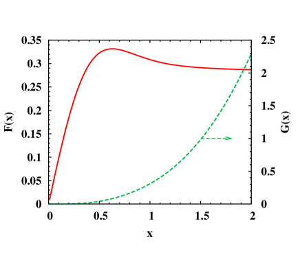
Figure 1: (Color online) $F(x)$ and $G(x)$ in Eq. (26). The scale of $G(x)$ is on the right-hand side of the frame.

III.2 Spin relaxation caused by the DP mechanism

In the analytical study, only the elastic spin-conserving scattering is considered. With the other spin-conserving scattering included, the spin relaxation rate due to the DP mechanism should be modified to be

$$\Gamma_{\rm DP}=4\lambda_{0}^{2}\tau_{p}^{\ast}(k_{f})/\hbar^{2},$$ (28)

where $\tau_{p}^{\ast}(k_{f})$ is the effective momentum relaxation time limited by all the different kinds of scattering, including the electron-electron Coulomb scattering.wu-review When $\lambda_{0}$ is fixed, the electron density and temperature affect $\Gamma_{\rm DP}$ via $\tau_{p}^{\ast}(k_{f})$. It has been shown previouslyyzhou that with the increase of $n_{e}$ or the decrease of $T$, the scattering strength decreases and $\Gamma_{\rm DP}$ increases. However, when the electron-impurity scattering is dominant, $\Gamma_{\rm DP}$ is insensitive to $T$. The dependence of $\Gamma_{\rm DP}$ on $n_{i}^{a}$ is not obvious. To facilitate the investigation, we write ${\tau_{p}^{\ast}}^{-1}(k_{f})=\tau_{p,i}^{-1}(k_{f})+\tau_{p,a}^{-1}(k_{f})$, where $\tau_{p,a}^{-1}(k_{f})$ is contributed by the electron-charged adatom scattering and $\tau_{p,i}^{-1}(k_{f})$ by all the other scattering. From Eq. (24), one has

$$\tau_{p,a}^{-1}(k_{f})=\frac{n_{i}^{a}k_{f}}{4\pi\hbar^{2}v_{f}}\int_{0}^{2\pi}d\theta|U^{a}_{\bf q}|^{2}\sin^{2}\theta\equiv c_{1}n_{i}^{a}$$ (29)

with $|{\bf q}|=2k_{f}\sin\frac{\theta}{2}$. With $\lambda_{0}=\lambda_{0}^{i}+2\pi n_{i}^{a}\overline{\delta}\xi^{2}\equiv\lambda_{0}^{i}+c_{2}n_{i}^{a}$, $\Gamma_{\rm DP}$ can be written as

$$\Gamma_{\rm DP}=\frac{4}{\hbar^{2}}\frac{(\lambda_{0}^{i}+c_{2}n_{i}^{a})^{2}}{\tau_{p,i}^{-1}(k_{f})+c_{1}n_{i}^{a}},$$ (30)

which indicates a complex dependence on $n_{i}^{a}$. When $c_{2}=0$ and $\lambda_{0}^{i}\neq 0$, $c_{2}>0$ and $0\leq n_{i}^{a}\leq c_{2}^{-1}\lambda_{0}^{i}-2c_{1}^{-1}\tau_{p,i}^{-1}(k_{f})$ or $c_{2}<0$ and $0\leq n_{i}^{a}\leq-c_{2}^{-1}\lambda_{0}^{i}$, $\Gamma_{\rm DP}$ decreases with increasing $n_{i}^{a}$, exhibiting the DP-like behaviour. However, most interestingly, when $c_{2}>0$ and $n_{i}^{a}\geq c_{2}^{-1}\lambda_{0}^{i}-2c_{1}^{-1}\tau_{p,i}^{-1}(k_{f})$ or $c_{2}<0$ and $n_{i}^{a}\geq-c_{2}^{-1}\lambda_{0}^{i}$, $\Gamma_{\rm DP}$ increases with increasing $n_{i}^{a}$, exhibiting the EY-like behaviour. Particularly, here in the limit with $n_{i}^{a}$ being large enough, $\Gamma_{\rm DP}\propto n_{i}^{a}$ approximately. With typical values in the presence of adatoms,zhanggraphene $\lambda_{0}=0.2$ meV and $\tau_{p}^{\ast}(k_{f})=0.1$ ps, $\Gamma_{\rm DP}^{-1}$ is calculated to be about 100 ps.

III.3 Comparison of relaxations caused by the spin-flip scattering due to the RRF and the DP mechanism

In this subsection we discuss the relative importance of the mechanism of spin-flip scattering due to the RRF and the DP mechanism in the regime with $k_{f}\xi\ll 1$, which is typically realized in graphene. Under this condition, from Eqs. (27) and (30), one obtains $\Gamma_{\rm DP}/\Gamma_{\rm flip}\approx 10{\overline{\delta}}^{2}/\overline{\delta^{2}}$ when $\lambda_{i}^{0}=\tau_{p,i}^{-1}(k_{f})=0$. For the case with single-sided adatoms, ${\overline{\delta}}^{2}=\overline{\delta^{2}}$, therefore $\Gamma_{\rm DP}/\Gamma_{\rm flip}\approx 10$ and $\Gamma_{\rm flip}$ can be neglected. However, for the case with double-sided adatoms, $\Gamma_{\rm flip}$ can be comparable to or even surpass $\Gamma_{\rm DP}$ as $\overline{\delta}$ may be as small as zero. In reality $\tau_{p,i}^{-1}(k_{f})\neq 0$ and $\Gamma_{\rm DP}$ decreases with increasing $\tau_{p,i}^{-1}(k_{f})$. When the substrate also contributes to the Rashba field as $\lambda_{i}^{0}$, $\Gamma_{\rm DP}$ can be either enhanced (e.g., when $\lambda_{i}^{0}\overline{\delta}>0$) or suppressed. As a consequence, for the configuration with single-sided adatoms, when the contribution from the substrate to the average Rashba field does not compensate that from the adatoms (e.g., when $\lambda_{i}^{0}\overline{\delta}\geq 0$) and the scattering other than the electron-adatom type is not extraordinarily strong (i.e., $\tau_{p,i}^{-1}$ is not unusually large), the spin relaxation caused by the spin-flip scattering due to the RRF can be neglected. In such a case, the spin relaxation is limited by the DP mechanism with the adatoms contributing to the average Rashba field. This is just how the effect of adatoms was incorporated in our previous investigation. zhanggraphene For other cases, whether the spin-flip scattering due to the RRF is important or not when compared to the DP mechanism is condition-dependent. Undoubtly, when the average Rashba field approaches zero, the spin-flip scattering due to the RRF tends to be important. In the work of Dugaev et al.,dugaev085306 the average Rashba field induced by ripples is zero and the spin relaxation is solely determined by the spin-flip scattering due to the RRF. However, the spin relaxation time calculated in their model is of the order of 10 ns, two orders of magnitude larger than the experimental values.

IV Numerical results

The KSBEs need to be solved numerically in order to take full account of all the different kinds of scattering. The initial conditions are set as

$$\rho_{\mu\bf k}(0)=\frac{f^{0}_{{\bf k}\uparrow}+f^{0}_{{\bf k}\downarrow}}{2}+\frac{f^{0}_{{\bf k}\uparrow}-f^{0}_{{\bf k}\downarrow}}{2}{\bf\hat{n}}\cdot{\mbox{\boldmath$\sigma$\unboldmath}},$$ (31)

$$\sum_{\mu\bf k}\mbox{Tr}[\rho_{\mu\bf k}(0){\bf\hat{n}}\cdot{\mbox{\boldmath$\sigma$\unboldmath}}]=n_{e}P(0),$$ (32)

$$\sum_{\mu\bf k}\mbox{Tr}[\rho_{\mu\bf k}(0)]=n_{e}.$$ (33)

At time $t=0$, the electrons are polarized along ${\bf\hat{n}}$ with the density and spin polarization being $n_{e}$ and $P(0)$, respectively. $f^{0}_{{\bf k}\uparrow/\downarrow}$ is the Fermi distribution function of electrons with spins parallel/antiparallel to ${\bf\hat{n}}$, where the chemical potential is determined by Eqs. (32)-(33). By solving the KSBEs, one can obtain the time evolution of spin polarization along ${\bf\hat{n}}$ as $P(t)=\frac{1}{n_{e}}\sum_{\mu\bf k}\mbox{Tr}[\rho_{\mu\bf k}(t){\bf\hat{n}}\cdot{\mbox{\boldmath$\sigma$\unboldmath}}]$ and hence the spin relaxation time $\tau_{s}$. In the calculation, we set $P(0)$ to be as small as 0.05 and ${\bf\hat{n}}$ in the graphene plane, such as, along the $y$-axis, in order to compare with experiments.

IV.1 Adatom density dependence of spin relaxation

In this section we study the adatom density dependence of spin relaxation based on the single-sided adatom model. In Fig. 2, the in-plane spin relaxation rate against the adatom density (at the top of the frame) or the inverse of charge diffusion coefficient (at the bottom of the frame) is shown. The temperature is $T=300$ K, the electron density is $n_{e}=10^{12}$ cm^-2, the density of impurities in the substrate is $n_{i}^{s}=0.2\times 10^{12}$ cm^-2 and the parameters for the single-sided adatom model are $\delta=5$ meV and $\xi=0.5$ nm. In the figure, the spin relaxation rates with different values of $\lambda_{0}^{i}$ are plotted by the curves. The nearby data points of each curve are calculated with the spin-flip scattering being removed. The small discrepancy between each curve and corresponding data points indicates that the DP mechanism dominates the spin relaxation. It is noted that in a large parameter regime of the background Rashba field $\lambda_{i}^{0}$, the curves show obvious EY-like behaviour, i.e., the spin relaxation rate is proportional to the momentum relaxation rate. When $\lambda_{i}^{0}$ is large enough [larger than $2c_{2}c_{1}^{-1}\tau_{p,i}^{-1}(k_{f})\approx 0.05$ meV from the discussion in Sec. III.2], the spin relaxation rate decreases with increasing adatom density at low doping density of adatoms, showing the DP-like behaviour.

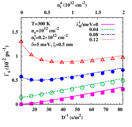
Figure 2: (Color online) The dependence of in-plane spin relaxation rate on the adatom density (at the top of the frame) or the inverse of the charge diffusion coefficient (at the bottom of the frame). The temperature is $T=300$ K, the electron density is $n_{e}=10^{12}$ cm^-2, the density of impurities in the substrate is $n_{i}^{s}=0.2\times 10^{12}$ cm^-2 and the parameters for the single-sided adatom model are $\delta=5$ meV and $\xi=0.5$ nm. The curves are calculated with different $\lambda_{0}^{i}$. For each curve, its nearby data points are calculated with the same parameters but without the spin-flip scattering.

We further apply the single-sided adatom model to reinvestigate the experiment of Pi et al. from Riverside,Pi which shows an obvious DP-like behaviour. At $T=18$ K, with the increasing density of adatoms (Au atoms) from surface deposition (although Au atoms also denote electrons to graphene, the electron density is fixed at 2.9$\times 10^{12}$ cm^-2 by adjusting the gate voltagePi ), the diffusion coefficient decreases while the spin relaxation time increases, as indicated by the crosses with error bars in Fig. 3. By fitting the experimental data without adatoms (before Au deposition), we obtain $\lambda_{i}^{0}=0.153$ meV and $n_{i}^{s}=2.1\times 10^{12}$ cm^-2.zhanggraphene During Au deposition, a group of parameters, $\delta=2.03$ meV and $\xi=0.5$ nm, can reproduce the experimental data except when the adatom density $n_{i}^{a}$ is larger than 2$\times 10^{12}$ cm^-2 (the solid curve). By assuming that $\xi$ decreases with the increase of $n_{i}^{a}$ when $n_{i}^{a}$ is large enough (the inset of Fig. 3), the recalculation can cover the experimental data in the region with large $n_{i}^{a}$ (the dashed curve). Similar to Fig. 2, the dots nearby the solid curve are calculated with the spin-flip scattering being removed (with $\xi$ being fixed as 0.5 nm). The small discrepancy between the solid curve and dots indeed indicates that the spin-flip scattering due to the RRF is not important.

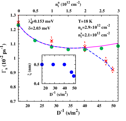
Figure 3: (Color online) The dependence of in-plane spin relaxation rate on the adatom density (at the top of the frame) or the inverse of the charge diffusion coefficient (at the bottom of the frame). The temperature is $T=18$ K, the electron density is $n_{e}=2.9\times 10^{12}$ cm^-2 and the density of impurities in the substrate is $n_{i}^{s}=2.1\times 10^{12}$ cm^-2. The crosses with error bars are the experimental data from Pi et al..Pi The solid curve stands for the fitting data via the single-sided adatom model with $\lambda_{0}^{i}=0.153$ meV, $\delta=2.03$ meV and $\xi=0.5$ nm. The nearby dots of the solid curve are calculated with the spin-flip scattering terms removed. The dashed curve is calculated with the same parameters as that of the solid curve except that $\xi$ decreases with $n_{i}^{a}$ when $n_{i}^{a}>2\times 10^{12}$ cm^-2, as shown in the inset.

IV.2 Electron density dependence of spin relaxation

The electron density dependence of spin relaxation is studied by fitting the experiment of Józsa et al. from Groningen,Jozsa_09 which shows an EY-like behaviour. At room temperature, with the increase of electron density from 0.16 to 2.81$\times 10^{12}$ cm^-2 (adjusted by the gate voltage), both the charge diffusion coefficient and the spin relaxation time increase, with the latter being proportional to the former (the squares in Fig. 4). It should be noted that this EY-like behaviour can not be explained by the nearly linear curves shown in Fig. 2, as the linearity there is due to the increase of adatom density when the electron density is fixed. In fact, according to Sec. III, with the increase of $n_{e}$ as well as the accompanying increase of $D$ [and hence the increase of $\tau_{p}^{\ast}(k_{f})$], both $\Gamma_{\rm flip}$ and $\Gamma_{\rm DP}$ should increase when the parameters for the adatom model are fixed [refer to Eqs. (27) and (30)]. However, as will be shown in the following, with the assumption that $\xi$ decreases with increasing $n_{e}$, both the single-sided and double-sided adatom models (hence both the DP mechanism and the mechanism of the spin-flip scattering due to the RRF) are able to fit the experimental data.

In Fig. 4, we present the fitting to the experimental data of Józsa et al. via the single-sided adatom model where the DP mechanism is dominant. The calculated spin relaxation time is plotted by the open circles in Fig. 4. The fitting parameters are chosen as $\lambda_{0}^{i}=0.127$ meV, $n_{i}^{a}=0.5\times 10^{12}$ cm^-2 and $\delta=4$ meV here. In order to reproduce the electron density dependence of diffusion coefficient, the impurity density in the substrate $n_{i}^{s}$ has to increase with increasing $n_{e}$ possibly due to the increased ionization (otherwise if $n_{i}^{s}$ is fixed, $D$ will increase with increasing $n_{e}$ much more quickly), as shown by the dots in the inset. Meanwhile, with the increase of $n_{e}$, $\xi$ should decrease as shown by the triangles in the inset (the scale is on the right-hand side of the frame) to account for the increase of $\tau_{s}$. Otherwise if $\xi$ is fixed, $\tau_{s}$ will decrease with increasing $D$ mainly due to the increase of $\Gamma_{\rm DP}$, as indicated by the dashed curve in the figure. In Fig. 5, we also present a feasible fitting by the double-sided adatom model. The squares stand for the experimental data and the open circles are from calculation. In our computation, $\lambda_{0}^{i}=0$, $n_{i}^{a}=0.5\times 10^{12}$ cm^-2 and $\delta_{1}=-\delta_{2}=5$ meV. The inset shows the dependences of $\xi$ (open triangles with the scale on the right-hand side of the frame) and $n_{i}^{s}$ (solid circles) on $D$ when $n_{e}$ is increased. In this fitting, only the spin-flip scattering due to the RRF plays a role in spin relaxation.

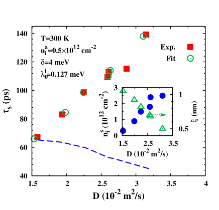
Figure 4: (Color online) Fit to the experimental data (the dependence of spin relaxation time $\tau_{s}$ on the charge diffusion coefficient $D$ with the increase of $n_{e}$) of Józsa et al.Jozsa_09 via the single-sided adatom model. The squares stand for the experimental data and the open circles are from our calculation. The inset shows the dependences of $\xi$ (with the scale on the right-hand side of the frame) and $n_{i}^{s}$ on $D$ when $n_{e}$ is increased. For comparison, the dashed curve is calculated with $\xi$ being fixed at 1.05 nm. $n_{i}^{a}=0.5\times 10^{12}$ cm^-2, $\lambda_{0}^{i}=0.127$ meV and $\delta=4$ meV.

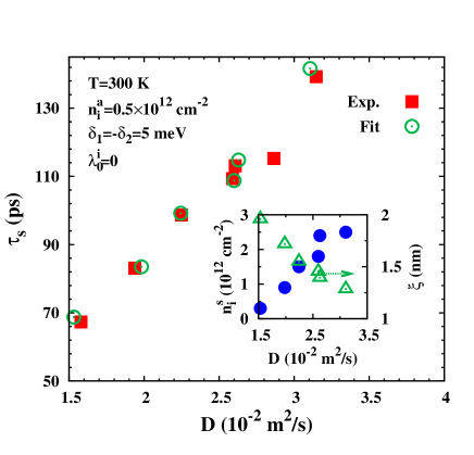
Figure 5: (Color online) Fit to the experimental data (the dependence of spin relaxation time $\tau_{s}$ on the charge diffusion coefficient $D$ with the increase of $n_{e}$) of Józsa et al.Jozsa_09 via the double-sided adatom model. The squares stand for the experimental data and the open circles are from our calculation. The inset shows the dependences of $\xi$ (with the scale on the right-hand side of the frame) and $n_{i}^{s}$ on $D$ when $n_{e}$ is increased. $n_{i}^{a}=0.5\times 10^{12}$ cm^-2, $\lambda_{0}^{i}=0$ and $\delta_{1}=-\delta_{2}=5$ meV.

IV.3 Temperature dependence of spin relaxation

We investigate the temperature dependence of spin relaxation in graphene in this section. Although the spin relaxation time determined by the DP mechanism increases with growing $T$ as pointed out in Sec. III, this dependence becomes very week when the electron-impurity scattering is dominant (which is satisfied in graphene on SiO₂ substrate), as revealed in Fig. 1 of Ref. yzhou, (note the mobility there is even one order of magnitude larger than the ones in this investigation). The spin relaxation time determined by the spin-flip scattering due to the RRF is also insensitive to $T$, as shown in Fig. 6. Therefore, when other parameters are fixed, the spin relaxation in graphene is expected to depend on temperature weakly.

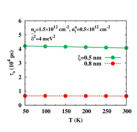
Figure 6: (Color online) Temperature dependence of spin relaxation time due to the spin-flip scattering. The parameters are $n_{e}=1.5\times 10^{12}$ cm^-2, $n_{i}^{a}=0.5\times 10^{12}$ cm^-2 and $\bar{\delta^{2}}=4$ meV². Solid curve: $\xi=0.5$ nm; and dotted curve: $\xi=0.8$ nm.

It is quite interesting that a decrease of $\tau_{s}$ with $T$ is observed by the Riverside group very recently.han1012.3435 Moreover, when $T$ is fixed, with the increase of $n_{e}$ (adjusted by the gate voltage), both $D$ and $\tau_{s}$ increase, similar to the observations by Józsa et al..Jozsa_09 The decrease of $\tau_{s}$ with growing $T$ may be due to the increase of the correlation length $\xi$ of the RRF with the increase of $T$, with either the DP mechanism or the spin-flip scattering due to the RRF being dominant. The linear scaling between $\tau_{s}$ and $D$ with the variation of electron density also can not determine which mechanism is the dominant one, as demonstrated in the previous section.

As a feasible way, we fit the temperature dependence of spin relaxation based on the single-sided adatom model by assuming $\xi$ to increase with $T$. One possible fitting is shown in Fig. 7. Experimentally, when the gate voltage $V_{\rm CNP}=20$ V (60 V), the electron density $n_{e}=1.47\times 10^{12}$ cm^-2 ($4.42\times 10^{12}$ cm^-2).illu In Fig. 7(a) and (b), the squares (open circles) are the experimental data of spin relaxation time and diffusion coefficient with $V_{\rm CNP}=20$ V (60 V), respectively, and the solid (dashed) curves are from our calculation with $V_{\rm CNP}=20$ V (60 V). The fitting parameters are $n_{i}^{a}=0.5\times 10^{12}$ cm^-2, $\lambda_{0}^{i}=0.052$ meV and $\delta=2$ meV. The variation of $\xi$ with $T$ is shown in Fig. 7(c), where the solid (dashed) curve is for $V_{\rm CNP}=20$ V (60 V). The variation of $n_{i}^{s}$ with $T$ is also shown in Fig. 7(c) with the scale on the right-hand side of the frame, where the dotted (chain) curve is for $V_{\rm CNP}=20$ V (60 V). In this fitting, the DP mechanism is dominant and the spin-flip scattering due to the RRF can be neglected. In fact, the calculation with similar parameters in Fig. 6 has indicated that the spin relaxation time caused by the spin-flip scattering due to the RRF is very long. With the same parameters, we further fit the dependence of spin relaxation time on diffusion coefficient at 100 K in Fig. 8. In consistence to the fittings in the previous section, the correlation length of the RRF is also found to decrease with increasing electron density. It is noted that the open squares in the figure are the data measured for holes or near the charge neutrality pointhan1012.3435 and hence are not considered in our fitting.

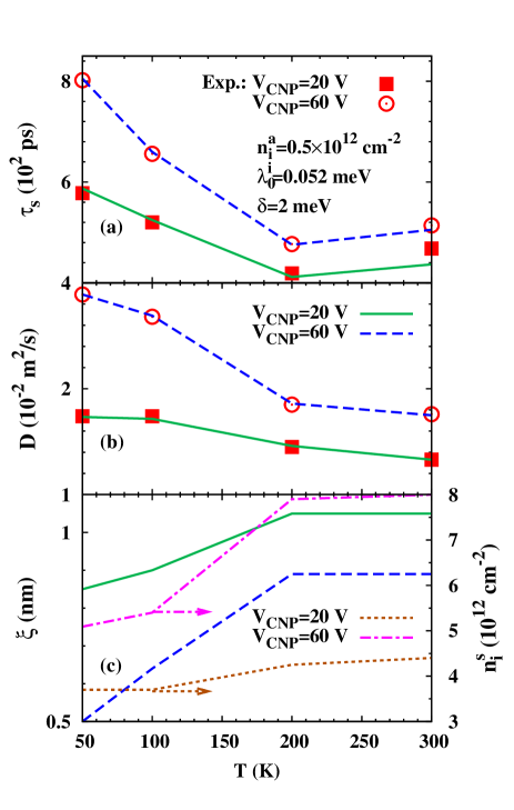
Figure 7: (Color online) Fit to the experimental data of Han and Kawakamihan1012.3435 with the single-sided adatom model. (a) and (b): the temperature dependence of $\tau_{s}$ and $D$. The squares (open circles) are the experimental data with $V_{\rm CNP}=20$ V (60 V), and the solid (dashed) curve is from fitting with $V_{\rm CNP}=20$ V (60 V). (c): the temperature dependences of $\xi$ and $n_{i}^{s}$ (on the right-hand side of the frame). The solid and dotted curves are for the case with $V_{\rm CNP}=20$ V, and the dashed and chain curves are for the case with $V_{\rm CNP}=60$ V.

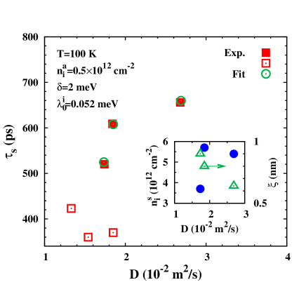
Figure 8: (Color online) Fit to the experimental data (the dependence of spin relaxation time $\tau_{s}$ on the charge diffusion coefficient $D$ with the increase of $n_{e}$) of Han and Kawakamihan1012.3435 via the single-sided adatom model. The solid squares stand for the experimental data and the open circles are from our calculation. The inset shows the dependences of $\xi$ (with the scale on the right-hand side of the frame) and $n_{i}^{s}$ on $D$ when $n_{e}$ is increased. The open squares are the experimental data for holes or near the charge neutrality point, which are not considered in our fitting. $n_{i}^{a}=0.5\times 10^{12}$ cm^-2, $\lambda_{0}^{i}=0.052$ meV and $\delta=2$ meV.

IV.4 A nonmonotonic dependence of $\tau_{s}$ on $D$

In the experiments of both Riversidehan1012.3435 and GroningenJozsa_09 groups, the spin relaxation time $\tau_{s}$ is observed to depend on the diffusion coefficient $D$ monotonically. However, very recently, a nonmonotonic dependence of $\tau_{s}$ on $D$ with the increase of carrier density at $T=4.2$ K was reported by Jo et al..jo Although this phenomenon is reported at the hole band, we can treat it at the electron band by our model due to the electron-hole symmetry of band structure in graphene. In Fig. 9, we fit the experimental data by the single-sided adatom model with $n_{i}^{a}=0.5\times 10^{12}$ cm^-2, $\lambda_{0}^{i}=0.127$ meV and $\delta=4$ meV. The closed squares (solid triangles) are the experimental (fitting) data of the spin relaxation time $\tau_{s}$, and the open squares (solid circles) are the experimental (fitting) data of the diffusion coefficient $D$ (with the scale on the right-hand side of the frame). The inset shows the density dependence of $\xi$ (open triangles with the scale on the right-hand side of the frame) and $n_{i}^{s}$ (solid circles). Due to the slower decrease of $\xi$ and the faster increase of $n_{i}^{s}$ with increasing $n_{e}$, it is possible for $\tau_{s}$ to decrease with $n_{e}$ when the latter is large enough.

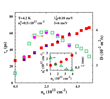
Figure 9: (Color online) Fit to the experimental data (the dependence of spin relaxation time $\tau_{s}$ and charge diffusion coefficient $D$ on electron density $n_{e}$) of Jo et al.jo via the single-sided adatom model. The closed squares (solid triangles) are the experimental (fitting) data of the spin relaxation time $\tau_{s}$, and the open squares (solid circles) are the experimental (fitting) data of the diffusion coefficient $D$ (with the scale on the right-hand side of the frame). The inset shows the density dependence of $\xi$ (with the scale on the right-hand side of the frame) and $n_{i}^{s}$. $n_{i}^{a}=0.5\times 10^{12}$ cm^-2, $\lambda_{0}^{i}=0.18$ meV and $\delta=6$ meV.

IV.5 Possible factors affecting the correlation length of the RRF

In our fittings to the experiments, the variation of the correlation length $\xi$ of the RRF plays an essential role. $\xi$ is found to decrease with increasing electron density and increase with growing temperature. $\xi$ is also found to decrease with the increase of adatom density when the latter is high enough. It is indeed quite possible that $\xi$ is affected by these factors. For example, the correlation length might be shortened by the screening of carriers, which is more effective when the carrier density is high. It is also possible that with growing temperature the adatoms tend to form clusters and enhance the inhomogeneity.mccreary Besides, the puddle size, which measures the correlation length of the short-range random potential in graphene, decreases with increasing density of the charged impurities.rossi The similar feature is also expected in the current study, i.e., $\xi$ decreases with increasing adatom density when the latter is large enough.

V Discussion and conclusion

V.1 Discussion on the possible dominant spin relaxation mechanism

We summarize our numerical fittings to the experiments and discuss the possible dominant spin relaxation mechanism. By fitting the DP-like behaviour with the increase of adatom density observed by the Riverside group,Pi we find that the DP mechanism is the dominant one, only with which can the experimental phenomenon be understood. It is noted that the correlation length $\xi$ of the RRF is supposed to be constant at the low density regime of adatoms, and when $\xi$ is fixed $\Gamma_{\rm flip}$ always increases with the adatom density. Therefore, other kinds of attempts with the spin-flip scattering due to the RRF being dominant fail to reproduce the experimental phenomenon and can be ruled out. However, the EY-like behaviour with the increase of electron density observed by the Groningen groupJozsa_09 can be fitted by our model with either the DP mechanism or the spin-flip scattering due to the RRF being dominant when the decrease of $\xi$ with increasing electron density is considered. Nevertheless, the fact that Riverside group has also observed the similar EY-like behaviour in their samples very recently,han1012.3435 in combination with the observation of the adatom density dependence of the spin relaxation,Pi suggests that the DP mechanism is dominant, but exhibiting EY-like properties with the increase of electron density. The similar experimental phenomenon on the electron density dependence of the spin relaxation from the GroningenJozsa_09 and Riversidehan1012.3435 groups further suggests that the DP mechanism also dominates the spin relaxation in the experiment of Groningen group.Jozsa_09 Consequently, with the DP mechanism being dominant in graphene, the RRF leads to spin relaxation which exhibits either DP- or EY-like properties in the experiments.

V.2 Conclusion

In conclusion, we have studied electron spin relaxation in graphene with random Rashba field by means of the kinetic spin Bloch equations, aiming to understand the main spin relaxation mechanism in graphene of the current experiments. Different from the previously studied case by Zhou and Wu where no adatoms are considered and the mobility is relatively high,yzhou ; novoselov666 the electron mobility investigated in the present work is at least one order of magnitude smaller due to the extrinsic factors caused by the ferromagnetic electrodes used in the spin relaxation measurements,Tombros_08 ; han222109 ; Popinciuc ; Jozsa_09 ; han1012.3435 ; jo e.g., the adatoms. We set up a random Rashba model to incorporate the contribution from both the adatoms and substrate. In this model, the charged adatoms on one hand enhance the Rashba spin-orbit coupling locally and on the other hand serve as Coulomb potential scatterers.

Based on the random Rashba model, the analytical study on spin relaxation in graphene is performed. The average of the random Rashba field leads to spin relaxation limited by the D’yakonov-Perel’ mechanism, which is absent in the work by Dugaev et al.,dugaev085306 while the randomness of the random Rashba field causes spin relaxation by spin-flip scattering, serving as an Elliott-Yafet–like mechanism. With the increase of adatom density, the spin relaxation caused by the spin-flip scattering due to the random Rashba field always shows an Elliott-Yafet–like behaviour, whereas the D’yakonov-Perel’ mechanism can exhibit either Elliott-Yafet– or D’yakonov-Perel’–like one. When all the other parameters are fixed, with the increase of electron density the spin relaxation rates due to both mechanisms increase; Nevertheless, the spin relaxation rate determined by the spin-flip scattering due to the random Rashba field is insensitive to the temperature whereas that determined by the D’yakonov-Perel’ mechanism becomes insensitive to the temperature when the electron-impurity scattering is dominant. However, both mechanisms are sensitive to the correlation length of the random Rashba field, which may be affected by the environmental factors such as electron density and temperature.

We further carry out numerical calculations and fit the experiments of RiversidePi ; han1012.3435 and GroningenJozsa_09 groups, which show either D’yakonov-Perel’– or Elliott-Yafet–like property. By fitting and comparing these experiments, we suggest that the D’yakonov-Perel’ mechanism dominates the spin relaxation in graphene. With the D’yakonov-Perel’ mechanism being dominant, the random Rashba field leads to spin relaxation which exhibits either D’yakonov-Perel’– or Elliott-Yafet–like properties. Besides, a latest reported nonmonotonic dependence of $\tau_{s}$ on $D$ by Jo et al.jo is also fitted by our model with the D’yakonov-Perel’ mechanism being dominant.

Appendix A Spin-flip scattering terms

The spin-flip scattering terms areglazov2157

$$\partial_{t}\rho_{\mu{\bf k}}(t)|_{\rm scat}^{f} = -\frac{\pi}{\hbar}\sum_{{\bf k}^{\prime}\neq{\bf k}}|\lambda_{\bf k-k^{\prime}}|^{2}\delta(\varepsilon_{\mu\bf k}-\varepsilon_{\mu\bf k^{\prime}})$$ (34)

$$\mbox{}\times[\rho_{\mu{\bf k}}(t)V_{\bf kk^{\prime}}V_{\bf k^{\prime}k}+V_{\bf kk^{\prime}}V_{\bf k^{\prime}k}\rho_{\mu{\bf k}}(t)$$

$$\mbox{}-2V_{\bf kk^{\prime}}\rho_{\mu{\bf k^{\prime}}}(t)V_{\bf k^{\prime}k}]$$

$$= -\frac{2\pi}{\hbar}\sum_{{\bf k}^{\prime}}|{\tilde{\lambda}}_{\bf k-k^{\prime}}|^{2}\delta(\varepsilon_{\mu\bf k}-\varepsilon_{\mu\bf k^{\prime}})$$

$$\mbox{}\times[\rho_{\mu{\bf k}}(t)-V_{\bf kk^{\prime}}\rho_{\mu{\bf k^{\prime}}}(t)V_{\bf k^{\prime}k}],$$

where

$${\tilde{\lambda}}_{\bf q} = \int[\lambda({\bf r})-\lambda_{0}]e^{-i{\bf q}\cdot{\bf r}}d{\bf r},$$ (35)

satisfying ${\tilde{\lambda}}_{{\bf q}=0}=0$ and ${\tilde{\lambda}}_{{\bf q}\neq 0}=\lambda_{{\bf q}}$. When the mean free path $l$ is much larger than the correlation length $\xi$ of the fluctuating Rashba field, $|{\tilde{\lambda}}_{\bf q}|^{2}$ can be approximated by its statistical average as follows,

$$|{\tilde{\lambda}}_{\bf q}|^{2} \approx \int\int d{\bf r}d{\bf r^{\prime}}\langle[\lambda({\bf r})-\lambda_{0}][\lambda({\bf r^{\prime}})-\lambda_{0}]\rangle$$ (36)

$$\mbox{}\times e^{-i{\bf q}\cdot({\bf r}-{\bf r^{\prime}})}$$

$$= \int\int d{\bf r}d{\bf r^{\prime}}C({\bf r}-{\bf r^{\prime}})e^{-i{\bf q}\cdot({\bf r}-{\bf r^{\prime}})}=C_{\bf q}.$$

Eqs. (34) and (36) lead to Eq. (12).

Appendix B Analytical study of spin relaxation in graphene

We present the analytical study of spin relaxation in graphene in detail. By expanding ${\bf S}_{\bf k}(t)$ as ${\bf S}_{\bf k}(t)=\sum_{l}{\bf S}_{k}^{l}(t)e^{il\theta_{\bf k}}$, one obtains from Eq. (14) the following equations,

$$\partial_{t}{S}^{l}_{kx}(t)= \frac{\lambda_{0}}{\hbar}\sum_{l_{0}=\pm 1}S_{kz}^{l+l_{0}}(t)-(\frac{1}{\tau_{k}^{l}}+\frac{1}{\tau_{ks}^{0}})S_{kx}^{l}(t)$$ (37)

$$\mbox{}-\sum_{l_{0}=\pm 1}\frac{S_{kx}^{l+2l_{0}}(t)+i^{l_{0}}S_{ky}^{l+2l_{0}}(t)}{2\tau_{ks}^{l+l_{0}}},$$

$$\partial_{t}{S}^{l}_{ky}(t)= \frac{\lambda_{0}}{\hbar}\sum_{l_{0}=\pm 1}i^{l_{0}}S_{kz}^{l+l_{0}}(t)-(\frac{1}{\tau_{k}^{l}}+\frac{1}{\tau_{ks}^{0}})S_{ky}^{l}(t)$$ (38)

$$\mbox{}-\sum_{l_{0}=\pm 1}\frac{i^{l_{0}}S_{kx}^{l+2l_{0}}(t)-S_{ky}^{l+2l_{0}}(t)}{2\tau_{ks}^{l+l_{0}}},$$

$$\partial_{t}{S}^{l}_{kz}(t)= -\frac{\lambda_{0}}{\hbar}\sum_{l_{0}=\pm 1}[S_{kx}^{l+l_{0}}(t)+i^{l_{0}}S_{ky}^{l+l_{0}}(t)]$$ (39)

$$\mbox{}-(\frac{1}{\tau_{k}^{l}}+\frac{2}{\tau_{ks}^{0}})S_{kz}^{l}(t),$$

in which

$$\frac{1}{\tau^{l}_{k}}=\frac{k}{4\pi\hbar^{2}v_{f}}\int_{0}^{2\pi}d\theta|U_{\bf q}|^{2}(1+\cos\theta)(1-\cos l\theta)$$ (40)

and

$$\frac{1}{\tau^{l}_{ks}}=\frac{k}{2\pi\hbar^{2}v_{f}}\int_{0}^{2\pi}d\theta C_{\bf q}\cos l\theta.$$ (41)

Here $|U_{\bf q}|^{2}$ and $C_{\bf q}$ depend only on $|{\bf q}|=2k\sin\frac{\theta}{2}$. It is noted that $\frac{1}{\tau^{l}_{k}}=\frac{1}{\tau^{-l}_{k}}$ and $\frac{1}{\tau^{l}_{ks}}=\frac{1}{\tau^{-l}_{ks}}$. It is also noted that $\frac{1}{\tau^{0}_{k}}=0$ and $\tau_{k}^{1}$ is in fact the momentum relaxation time $\tau_{p}(k)$ limited by the electron-impurity scattering.

By retaining the lowest three orders of ${\bf S}_{k}^{l}(t)$ (i.e., terms with $l=0$, $\pm 1$) in Eqs. (37)-(39), one obtains

$$\left[\partial_{t}-\left(\begin{array}[]{ccc}{\bf F}&{\bf P}&{\bf Q}\\ -{\bf P}^{\dagger}&{\bf G}&{\bf P}\\ {\bf Q}^{\dagger}&-{\bf P}^{\dagger}&{\bf F}\end{array}\right)\right]\left(\begin{array}[]{c}{\bf S}_{k}^{1}\\ {\bf S}_{k}^{0}\\ {\bf S}_{k}^{-1}\end{array}\right)=0,$$ (48)

where

$${\bf G}=-\frac{1}{\tau_{ks}^{0}}\left(\begin{array}[]{ccc}1&0&0\\ 0&1&0\\ 0&0&2\end{array}\right),$$ (52)

$${\bf F}={\bf G}-\frac{1}{\tau_{k}^{1}},$$ (53)

$${\bf P}=\frac{\lambda_{0}}{\hbar}\left(\begin{array}[]{ccc}0&0&1\\ 0&0&-i\\ -1&i&0\end{array}\right),$$ (57)

$${\bf Q}=\frac{1}{2\tau_{ks}^{0}}\left(\begin{array}[]{ccc}-1&i&0\\ i&1&0\\ 0&0&0\end{array}\right).$$ (61)

As the spin flipping rate $1/\tau_{ks}^{0}$ is much smaller than the momentum relaxation rate $1/\tau_{k}^{1}$ (in graphene $1/\tau_{k}^{1}$ is usually of the order of 10 ps^-1; even if $1/\tau_{ks}^{0}$ reaches the experimental value $\sim$ 0.01 ps^-1, $\tau_{k}^{1}/\tau_{ks}^{0}$ is still as small as 10^-3) and ${\bf S}_{k}^{\pm 1}$ are smaller terms compared to ${\bf S}_{k}^{0}$ in the strong scattering limit, we approximate ${\bf F}$ and ${\bf Q}$ as ${\bf F}\approx-\frac{1}{\tau_{k}^{1}}$ and ${\bf Q}\approx 0$. With initial conditions, e.g., ${\bf S}_{k}^{l}(0)=\delta_{l0}(0,0,S_{kz}^{0}(0))^{T}$ ($l=0,\pm 1$), Eq. (48) can be solved as [those of ${\bf S}_{k}^{\pm 1}(t)$ are away from our interest and are not shown here]

$${\bf S}_{k}^{0}(t) = \frac{1}{2}\Big{[}\Big{(}1+\frac{1}{\sqrt{1-c_{z}^{2}}}\Big{)}e^{-\Gamma_{z}^{+}t}+\Big{(}1-\frac{1}{\sqrt{1-c_{z}^{2}}}\Big{)}$$ (62)

$$\times e^{-\Gamma_{z}^{-}t}\Big{]}(0,0,S_{kz}^{0}(0))^{T},$$

where

$$c_{z}=\frac{4\lambda_{0}}{\hbar}\frac{1}{1/\tau_{k}^{1}-1/\tau_{ks}^{0}}$$ (63)

and

$$\Gamma_{z}^{\pm}=\frac{1}{\tau_{ks}^{0}}+\frac{1}{2\tau_{k}^{1}}\pm(\frac{1}{\tau_{ks}^{0}}-\frac{1}{2\tau_{k}^{1}})\sqrt{1-c_{z}^{2}}.$$ (64)

In the strong scattering limit with $c_{z}\ll 1$, $S_{kz}^{0}(t)\approx S_{kz}^{0}(0)e^{-\Gamma_{z}^{+}t}$ where $\Gamma_{z}^{+}\approx 2/\tau_{ks}^{0}+4\lambda_{0}^{2}\tau_{k}^{1}/\hbar^{2}$. Consequently, one obtains

$${\bf S}_{k}^{0}(t)=e^{-\Gamma_{z}t}(0,0,S_{kz}^{0}(0))^{T}$$ (65)

with

$$\Gamma_{z}=2/\tau_{ks}^{0}+4\lambda_{0}^{2}\tau_{k}^{1}/\hbar^{2}.$$ (66)

Similarly, with ${\bf S}_{k}^{l}(0)=\delta_{l0}(S_{kx}^{0}(0),0,0)^{T}$ or ${\bf S}_{k}^{l}(0)=\delta_{l0}(0,S_{ky}^{0}(0),0)^{T}$, ${\bf S}^{0}_{k}(t)$ is solved to be

$${\bf S}_{k}^{0}(t)=e^{-\Gamma_{x}t}(S_{kx}^{0}(0),0,0)^{T},$$ (67)

and

$${\bf S}_{k}^{0}(t)=e^{-\Gamma_{y}t}(0,S_{ky}^{0}(0),0)^{T},$$ (68)

respectively, with $\Gamma_{x}=\Gamma_{y}=\Gamma_{z}/2$.

References

- (1) K. S. Novoselov, A. K. Geim, S. V. Morozov, D. Jiang, Y. Zhang, S. V. Dubonos, I. V. Grigorieva, and A. A. Firsov, Science 306, 666 (2004).
- (2) A. K. Geim and K. S. Novoselov, Nature Mater. 6, 183 (2007).
- (3) N. Tombros, C. Józsa, M. Popinciuc, H. T. Jonkman, and B. J. van Wees, Nature (London) 448, 571 (2007).
- (4) F. Kuemmeth, S. Ilani, D. C. Ralph, and P. L. McEuen, Nature 452, 448 (2008).
- (5) A. H. Castro Neto, F. Guinea, N. M. R. Peres, K. S. Novoselov, and A. K. Geim, Rev. Mod. Phys. 81, 109 (2009).
- (6) N. M. R. Peres, Rev. Mod. Phys. 82, 2673 (2010).
- (7) E. R. Mucciolo and C. H. Lewenkopf, J. Phys.: Condens. Matter 22, 273201 (2010).
- (8) S. Das Sarma, S. Adam, E. H. Hwang, and E. Rossi, Rev. Mod. Phys. 83, 407 (2011).
- (9) D. H. Hernando, F. Guinea, and A. Brataas, Phys. Rev. B 74, 155426 (2006).
- (10) C. L. Kane and E. J. Mele, Phys. Rev. Lett. 95, 226801 (2005).
- (11) H. Min, J. E. Hill, N. A. Sinitsyn, B. R. Sahu, L. Kleinman, and A. H. MacDonald, Phys. Rev. B 74, 165310 (2006).
- (12) M. Gmitra, S. Konschuh, C. Ertler, C. A. Draxl, and J. Fabian, Phys. Rev. B 80, 235431 (2009).
- (13) S. Abdelouahed, A. Ernst, J. Henk, I. V. Maznichenko, and I. Mertig, Phys. Rev. B 82, 125424 (2010).
- (14) A. Varykhalov, J. S. Barriga, A. M. Shikin, C. Biswas, E. Vescovo, A. Rybkin, D. Marchenko, and O. Rader, Phys. Rev. Lett. 101, 157601 (2008).
- (15) A. H. Castro Neto and F. Guinea, Phys. Rev. Lett. 103, 026804 (2009).
- (16) S. Ryu, L. Liu, S. Berciaud, Y. J. Yu, H. Liu, P. Kim, G. W. Flynn, and L. E. Brus, Nano Lett. 10, 4944 (2010).
- (17) Y. S. Dedkov, M. Fonin, U. Rüdiger, and C. Laubschat, Phys. Rev. Lett. 100, 107602 (2008).
- (18) C. Ertler, S. Konschuh, M. Gmitra, and J. Fabian, Phys. Rev. B 80, 041405(R) (2009).
- (19) Y. A. Bychkov and E. I. Rashba, J. Phys. C 17, 6039 (1984).
- (20) N. Tombros, S. Tanabe, A. Veligura, C. Józsa, M. Popinciuc, H. T. Jonkman, and B. J. van Wees, Phys. Rev. Lett. 101, 046601 (2008).
- (21) W. Han, K. Pi, W. Bao, K. M. McCreary, Y. Li, W. H. Wang, C. N. Lau, and R. K. Kawakami, Appl. Phys. Lett. 94, 222109 (2009).
- (22) M. Popinciuc, C. Józsa, P. J. Zomer, N. Tombros, A. Veligura, H. T. Jonkman, and B. J. van Wees, Phys. Rev. B 80, 214427 (2009).
- (23) C. Józsa, T. Maassen, M. Popinciuc, P. J. Zomer, A. Veligura, H. T. Jonkman, and B. J. van Wees, Phys. Rev. B 80, 241403(R) (2009).
- (24) K. Pi, W. Han, K. M. McCreary, A. G. Swartz, Y. Li, and R. K. Kawakami, Phys. Rev. Lett. 104, 187201 (2010).
- (25) T.-Y. Yang, J. Balakrishnan, F. Volmer, A. Avsar, M. Jaiswal, J. Samm, S. R. Ali, A. Pachoud, M. Zeng, M. Popinciuc, G. Güntherodt, B. Beschoten, and B. Özyilmaz, Phys. Rev. Lett. 107, 047206 (2011).
- (26) W. Han and R. K. Kawakami, Phys. Rev. Lett. 107, 047207 (2011).
- (27) S. Jo, D. K. Ki, D. Jeong, H. J. Lee, and S. Kettemann, Phys. Rev. B 84, 075453 (2011).
- (28) M. I. D’yakonov and V. I. Perel’, Zh. Éksp. Teor. Fiz. 60, 1954 (1971) [Sov. Phys. JETP 33, 1053 (1971)].
- (29) R. J. Elliott, Phys. Rev. 96, 266 (1954); Y. Yafet, Phys. Rev. 85, 478 (1952).
- (30) D. H. Hernando, F. Guinea, and A. Brataas, Phys. Rev. Lett. 103, 146801 (2009).
- (31) Y. Zhou and M. W. Wu, Phys. Rev. B 82, 085304 (2010).
- (32) V. K. Dugaev, E. Ya. Sherman, and J. Barnas, Phys. Rev. B 83, 085306 (2011).
- (33) H. Ochoa, A. H. Castro Neto, and F. Guinea, arXiv:1107.3386.
- (34) P. Zhang and M. W. Wu, Phys. Rev. B 84, 045304 (2011).
- (35) Private communication with W. Han.
- (36) E. Ya. Sherman, Phys. Rev. B 67, 161303 (2003).
- (37) E. Ya. Sherman, Appl. Phys. Lett. 82, 209 (2003).
- (38) For review: M. M. Glazov, E. Ya. Sherman, and V. K. Dugaev, Physica E 42, 2157 (2010).
- (39) Y. Zhou and M. W. Wu, Europhys. Lett. 89, 57001 (2010).
- (40) M. W. Wu, J. H. Jiang, and M. Q. Weng, Phys. Rep. 493, 61 (2010).
- (41) C. H. Lewenkopf, E. R. Mucciolo, and A. H. Castro Neto, Phys. Rev. B 77, 081410 (2008).
- (42) S. Adam and S. Das Sarma, Solid State Commun. 146, 356 (2008).
- (43) K. M. McCreary, K. Pi, A. G. Swartz, W. Han, W. Bao, C. N. Lau, F. Guinea, M. I. Katsnelson, and R. K. Kawakami, Phys. Rev. B 81, 115453 (2010).
- (44) M. Lazzeri, S. Piscanec, F. Mauri, A. C. Ferrari, and J. Robertson, Phys. Rev. Lett. 95, 236802 (2005).
- (45) E. H. Hwang and S. Das Sarma, Phys. Rev. B 77, 115449 (2008).
- (46) S. Fratini and F. Guinea, Phys. Rev. B 77, 195415 (2008).
- (47) The electron density is obtained from the arXiv version of Ref. han1012.3435, (arXiv:1012.3435).
- (48) E. Rossi and S. Das Sarma, Phys. Rev. Lett. 101, 166803 (2008).