Entangled spin-orbital phases in the bilayer Kugel-Khomskii model

Abstract

We derive the Kugel-Khomskii spin-orbital model for a bilayer and investigate its phase diagram depending on Hund’s exchange $J_{H}$ and the $e_{g}$ orbital splitting $E_{z}$. In the (classical) mean-field approach with on-site spin $\langle S_{i}^{z}\rangle$ and orbital $\langle\tau_{i}^{z}\rangle$ order parameters and factorized spin-and-orbital degrees of freedom, we demonstrate a competition between the phases with either $G$-type or $A$-type antiferromagnetic (AF) or ferromagnetic long-range order. Next we develop a Bethe-Peierls-Weiss method with a Lanczos exact diagonalization of a cube coupled to its neighbors in $ab$ planes by the mean-field terms — this approach captures quantum fluctuations on the bonds which decide about the nature of disordered phases in the highly frustrated regime near the orbital degeneracy. We show that the long-range spin order is unstable in a large part of the phase diagram which contains then six phases, including also the valence-bond phase with interlayer spin singlets stabilized by holes in $3z^{2}-r^{2}$ orbitals (VB$z$ phase), a disordered plaquette valence-bond (PVB) phase and a crossover phase between the VB$z$ and the $A$-type AF phase. When on-site spin-orbital coupling is also included by the $\langle S_{i}^{z}\tau_{i}^{z}\rangle$ order parameter, we discover in addition two entangled spin-disordered phases which compete with $A$-type AF phase and another crossover phase in between the $G$-AF phase with occupied $x^{2}-y^{2}$ orbitals and the PVB phase. Thus, the present bilayer model provides an interesting example of spin-orbital entanglement which generates novel disordered phases. We analyze the order parameters in all phases and identify situations where spin-orbital entanglement is crucial and mean-field factorization of the spin and orbital degrees of freedom leads to qualitatively incorrect results. We point out that spin-orbital entanglement may play a role in a bilayer fluoride K₃Cu₂F₇ which is an experimental realization of the VB$z$ phase.
Published in: Physical Review B 83, 214408 (2011).

I Introduction

Recent interest and progress in the theory of spin-orbital superexchange models was triggered by the observation that orbital degeneracy drastically increases quantum fluctuations which may suppress long-range order in the regime of strong competition between different types of ordered states near the quantum critical point.Fei97 The simplest model of this type is the Kugel-Khomskii ($d^{9}$) model introduced long agoKug82 for KCuF₃, a strongly correlated system with a single hole within degenerate $e_{g}$ orbitals at each Cu²⁺ ion. Kugel and Khomskii showed that many-body effects could then give rise to orbital order stabilized by a purely electronic superexchange mechanism. A similar situation occurs in a number of compounds with active orbital degrees of freedom, where strong on-site Coulomb interactions localize electrons (or holes) and give rise to spin-orbital superexchange. Nag00 ; Kha05 ; Hfm The orbital superexchange may stabilize the orbital order by itself, but in $e_{g}$ systems it is usually helped by the orbital interactions which follow from the Jahn-Teller distortions of the lattice.Kug82 ; Zaa93 ; Fei99 ; Ole05 For instance, in LaMnO₃ these contributions are of equal importance and both of them are necessary to explain the observed high temperature of the structural transition.Fei99 Also in KCuF₃ the lattice distortions play an important role and explain its strongly anisotropic magnetic and optical properties. Ole05 ; Dei08 ; Leo10

An important feature of spin-orbital superexchange, which arises in transition metal oxides with active orbital degrees of freedom, Kug82 ; Nag00 ; Kha05 ; Hfm is generic frustration of the orbital part of the superexchange. It follows from the directional nature of orbital interactions,Fei97 which is in contrast to the SU(2) symmetry of spin interactions. Therefore, the orbital part of the spin-orbital superexchange is intrinsically frustrated also on lattices without geometrical frustration, such as the three-dimensional (3D) perovskite lattice of KCuF₃ or LaMnO₃. Generic features of this direction-dependent orbital interactions are best captured within the two-dimensional (2D) quantum compass model, Nus04 which exhibits a quantum phase transition from one to the other one-dimensional (1D) columnar order through a point with isotropic and strongly frustrated interactions.Wen08 ; Oru09 In spite of the intrinsic frustration and high degeneracy of the ground state, the long-range order of 1D type exists in the 2D quantum compass model, as shown by a rigorous proof.You10 Numerical simulations demonstrate that this model is in the universality class of the 2D Ising modelNus08 and the order persists in a range of finite temperature.Wen08 In contrast, the superexchange interactions for the 2D $e_{g}$ orbital model contain orbital quantum fluctuations on the bonds,Fei97 ; vdB99 but nevertheless the long-range order survives also in this case.You07

An intriguing situation arises when spin and orbital part of the superexchange are strongly coupled and compete with each other, as found in realistic spin-orbital models for several transition metal oxides.Kha05 ; Hfm For instance, a qualitatively new spin-orbital liquid phase may arise when the superexchange interactions are geometrically frustrated on the triangular lattice,Nor08 or spin order cannot stabilize in LiNiO₂, another compound with triangular lattice of magnetic, in spite of presence of strong orbital interactions which suggest pronounced orbital order.Ver04 A more standard situation is found in the transition metal oxides which crystallize in the perovskite lattice, where in general spin order coexists with orbital order, Nag00 ; Kha05 ; Hfm and both satisfy the classical Goodenough-Kanamori rules.Goode A well known example is the archetypical compound with degenerate $e_{g}$ orbitals, KCuF₃, in which the orbital order is stabilized jointly by the superexchange and Jahn-Teller lattice distortions.Ole05 ; Leo10 As a result, the magnetic interactions are strongly anisotropic and give rise to quasi-1D Heisenberg antiferromagnetic (AF) chain dominated by quantum fluctuations and characterized by spinon excitations, Ten93 with a dimensional crossover occurring when temperature is lowered below the Néel temperature $T_{N}$.Lak05

While the coexisting $A$-type AF ($A$-AF) order and the orbital order is well established in KCuF₃ below $T_{N}$,Cuc02 and this phase is reproduced by the spin-orbital $d^{9}$ superexchange model,Ole00 the model poses an interesting question by itself: Which types of coexisting spin and orbital order (or disorder) are possible when its microscopic parameters are varied? So far, it was only established that the long-range AF order is destroyed by strong quantum fluctuations,Ole00 ; Fei98 and it has been shown that instead certain spin disordered phases with valence-bond (VB) correlations stabilized by local orbital correlations are favored. Fei97 ; Kha05 However, the phase diagram of the Kugel-Khomskii $d^{9}$ model is unknown — it was not studied systematically beyond the mean-field (MF) approximation and certain simple variational wave functions and it remains an outstanding problem in the theory.Fei97

The purpose of this paper is to analyze a simpler situation of the spin-orbital Kugel-Khomskii model for a bilayer, called below bilayer spin-orbital $d^{9}$ model, consisting of two $ab$ layers connected by interlayer bonds along the $c$ axis. This choice is motivated by an expected competition of the long-range AF order with VB-like states. One of them, a VB phase with spin singlets on the interlayer bonds (VB$z$ phase), is stabilized by large crystal field $E_{z}$ which favors occupied $3z^{2}-r^{2}$ orbitals (by holes). We shall investigate the range of stability of this and other phases, including the $A$-AF phase similar to the one found in KCuF₃.

To establish reliable results concerning short-range order in the crossover regime between phases with long-range AF or FM order, we developed a cluster MF approach which goes beyond the single site MF in the spin-orbital systemDeS03 and is based on an exact diagonalization of an eight-site cubic cluster coupled to its neighbors by MF terms. This unit is sufficient for investigating both AF phases with four sublattices and VB states, with spin singlets either along the $c$ axis or within the $ab$ planes. This theoretical method is motivated by possible spin-orbital entanglementOle06 which is particularly pronounced in the 1D SU(4) [or SU(2)$\otimes$SU(2)] spin-orbital models,Fri99 and occurs also in the models for perovskites with AF spin correlations on the bonds where it violates the Goodenough-Kanamori rules. Goode In the perovskite vanadates such entangled states play an important role in their optical properties,Kha04 in the phase diagramHor08 and in the dimerization of FM interactions along the $c$ axis in the $C$-AF phase of YVO₃.Ulr03 ; Sir08 Below we shall investigate whether entangled states could play a role in the present Kugel-Khomskii model for a bilayer with nearly degenerate $e_{g}$ orbitals. Thereby we establish exotic type of spin-orbital order stabilized by joint quantum spin-orbital fluctuations, and investigate signatures of entangled states in this phase.

The paper is organized as follows. In Sec. II we present the Kugel-Khomskii $d^{9}$ spin-orbital model for a bilayer which consists of two 2D square lattices in $ab$ planes coupled by vertical bonds along the $c$ axis. First in Sec. II.1 we introduce the $d^{9}$ spin-orbital model for a bilayer derived here following Ref. Ole00, . Its classical phase diagram obtained in a single-site MF approximation is presented in Sec. II.2. Next we argue that quantum fluctuations and intrinsic frustration of the superexchange near the orbital degeneracy motivate the solution of this model in a better MF approximation based on an embedded cubic cluster, which we introduce in Sec. II.3. It leads to MF equations which were solved self-consistently in an iterative way, as described in Sec. II.4. In Sec. III we present two phase diagrams obtained from the MF analysis using Bethe-Peierls-Weiss cluster method: (i) the phase diagram which follows from factorization of spin and orbital degrees of freedom in Sec. III.1, and (ii) the one obtained when also on-site joint on-site spin-orbital order parameter is introduced, see Sec. III.2. The latter approach gives nine different phases, and we describe characteristic features of their order parameters in Sec. IV. We introduce bond correlation functions in Sec. V.1, and concentrate their analysis on the regime of almost degenerate $e_{g}$ orbitals, focusing on the proximity of the plaquette VB (PVB) and entangled spin-orbital (ESO) phases in Secs. V.2 and V.3. Finally, we quantify the spin-orbital entanglement using on-site and bond correlations, see Sec. VI, which modifies significantly the phase diagram of the model with respect to the one obtained when spin and orbital operators are disentangled. General discussion and summary are presented in Sec. VII.

II Spin-orbital model and methods

II.1 Kugel-Khomskii model for a bilayer

For realistic parameters the late transition metal oxides or fluorides are strongly correlated and electrons localize in the $3d$ orbitals, Ole87 ; Gra92 leading to Cu²⁺ ions with spin $S=1/2$ in $d^{9}$ configuration, as e.g. in KCuF₃ or La₂CuO₄. The virtual charge excitations lead then to superexchange which involves also orbital degrees of freedom in systems with partly filled degenerate orbitals. In analogy to the models introduced for bilayer manganite,Ole03 ; Dag06 La_2-xSr_xMn₂O₇, we consider here a model for K₃Cu₂F₇ bilayer compound, with two active and nearly degenerate $e_{g}$ orbitals,

$$|x\rangle\equiv(x^{2}-y^{2})/\sqrt{2},\hskip 19.91684pt|z\rangle\equiv(3z^{2}-r^{2})/\sqrt{6}\,,$$ (1)

while $t_{2g}$ orbitals do not contribute and are filled with electrons. They do not couple to $e_{g}$’s by hopping through fluorine and hence can be neglected. We investigate in what follows an electronic model and neglect coupling to the lattice distortions arising due to Jahn-Teller effect. The bilayer K₃Cu₂F₇ system is known since twenty years,Von81 but its magnetic properties were reported only recently.Man07 We shall address the orbital order and magnetic correlations realized in this system below.

The Hamiltonian for $d^{9}$ systems contains: holes’ kinetic energy $H_{t}$ with hopping amplitude $t$, electron-electron interactions $H_{\rm int}$, with on-site Hubbard $U$ and Hund’s exchange coupling $J_{H}$, as well as crystal-field splitting term $H_{z}$ playing a role of external orbital field $E_{z}$ acting on $e_{g}$ orbitals:

$$H_{e_{g}}=H_{t}+H_{\rm int}+H_{z}.$$ (2)

Because of the shape of the two $e_{g}$ orbitals Eq. (1), the effective hopping elements are direction dependent and different depending on the direction of the bond $\langle ij\rangle$. The only non-vanishing $(dd\sigma)$ hopping element in the $c$ direction connects two $|z\rangle$ orbitals,Zaa93 while the elements in the $ab$ planes satisfy Slater-Koster relations.

Taking the effective $(dd\sigma)$ hopping element $t$ for two $z$ orbitals on a bond along the $c$ axis as a unit, $H_{t}$ is given by

$$H_{t} = \frac{t}{4}\!\sum_{\langle ij\rangle\parallel ab}\left\{3d^{\dagger}_{ix\sigma}d_{jx\sigma}+d^{\dagger}_{ix\sigma}d_{jz\sigma})\right.$$ (3)

$$\left.\hskip 34.14322pt\pm\sqrt{3}(d^{\dagger}_{iz\sigma}d_{jx\sigma}+d^{\dagger}_{ix\sigma}d_{jz\sigma})+{\rm H.c.}\right\}$$

$$+ t\sum_{\langle ij\rangle\parallel c}(d^{\dagger}_{iz\sigma}d_{jz\sigma}+{\rm H.c.}),$$

where $d^{\dagger}_{ix\sigma}$ and $d^{\dagger}_{iz\sigma}$ are creation operators for a hole in $x$ and $z$ orbital with spin $\sigma=\uparrow,\downarrow$, and the in-plane $x$–$z$ hopping depends on the phase of $|x\rangle$ orbital involved in the hopping process along the bond $\langle ij\rangle$ and is included in the alternating sign of the terms $\propto\sqrt{3}$ between $a$ and $b$ cubic axes. The on-site electron-electron interactions are described by:Ole83

$$H_{\rm int} = U\sum_{i\alpha}n_{i\alpha\uparrow}n_{i\alpha\downarrow}+(U-3J_{H})\sum_{i\sigma}n_{ix\sigma}n_{iz\sigma}$$ (4)

$$+ (U-2J_{H})\sum_{i\sigma}n_{ix\sigma}n_{iz\bar{\sigma}}-J_{H}\!\sum_{i\sigma}\!d^{\dagger}_{ix\sigma}d_{ix\bar{\sigma}}d^{\dagger}_{iz\bar{\sigma}}d_{iz\sigma}$$

$$+ J_{H}\!\sum_{i}(d^{\dagger}_{ix\uparrow}d^{\dagger}_{ix\downarrow}d_{iz\downarrow}d_{iz\uparrow}+H.c.)\,.$$

Here $n_{i\alpha\sigma}$ stands for the hole density operator in orbital $\alpha=x,z$ with spin $\sigma$, and $\bar{\sigma}=-\sigma$. This Hamiltonian describes the multiplet structure of $d^{8}$ or $d^{2}$ ions and is rotationally invariant in the orbital space. We assumed the wave function to be real which gives the same amplitude $J_{H}$ for Hund’s exchange interaction and for pair hopping term between $|x\rangle$ and $|z\rangle$ orbitals. The last term of the $H_{e_{g}}$ Hamiltonian lifts the degeneracy of the two $e_{g}$ orbitals

$$H_{z}=-\frac{1}{2}E_{z}\sum_{i\sigma}(n_{ix\sigma}-n_{iz\sigma}),$$ (5)

and favors hole occupancy of $x$ ($z$) orbitals when $E_{z}>0$ ($E_{z}<0$). It can be associated with a uniaxial pressure along the $c$ axis, induced by the bilayer geometry or by external pressure.

The typical energies for the Coulomb $U$ and Hund’s exchange $J_{H}$ elements can be deduced from the atomic spectra or found using density functional theory with constrained electron densities. Earlier studies performed within the local density approximation (LDA) gave rather large values of the interaction parameters:Gra92 $U=8.96$ eV and $J_{H}=1.19$ eV. More recent studies used the LDA with on-site Coulomb interaction treated within the LDA+$U$ scheme and gave somewhat reduced values:Lic95 $U=7.5$ eV and $J_{H}=0.9$ eV. However, both parameter sets give rather similar values of Hund’s exchange parameter,

$$\eta=\frac{J_{H}}{U},$$ (6)

being close to 0.13 or 0.12, i.e., within the expected range $0.1<\eta<0.2$ for strongly correlated late transition metal oxides. Note that the physically acceptable range which follows from Eq. (4) is much broader, i.e., $0<\eta<1/3$.

The value of effective intersite $(dd\sigma)$ hopping element $t$ is more difficult to estimate. It follows from the usual effective process via the oxygen orbitals described by a $t_{pd}$ hopping, and the energy difference between the $3d$ and $2p$ orbitals involved in the hopping process, so-called charge-transfer energy.Zaa93 A representative value of $t\simeq 0.65$ eV may be derived from the realistic parameters Gra92 of CuO₂ planes in La₂CuO₄. Taking in addition $U=7.5$ eV, one finds the superexchange constant between hole $S=1/2$ spins within $|x\rangle$ orbitals in a single CuO₂ plane, $J_{x}=(9/4)t^{2}/U\simeq 0.127$ eV, which reproduces well the experimental value, as discussed in Ref. Ole00, .

Thanks to $t\ll U$ we can safely assume that the ground state is insulating at the filling of one hole localized at each Cu²⁺ ion. In the atomic limit ($t=0$ and $E_{z}=0$) we have large $4^{N}$-fold degeneracy as the hole can occupy either $x$ or $z$ orbital and have up or down spin. This high degeneracy is lifted due to effective superexchange interactions between spins and orbitals at nearest neighbor Cu ions $i$ and $j$ which act along the bond $\langle ij\rangle$. They originate from the virtual transitions to the excited states, i.e., $d^{9}_{i}d^{9}_{j}\rightleftharpoons d^{10}_{i}d^{8}_{j}$, and are generated by the hopping term Eq. (3). Hence, the effective spin-orbital model can be derived from the atomic limit Hamiltonian containing interaction Eq. (4) and the crystal-field term Eq. (5), treating the kinetic term Eq. (3) as a perturbation. Taking into account the full multiplet structure of the excited states for the $d^{8}$ configuration,Ole00 one gets the corrections of the order of $J_{H}$ to the Hamiltonian which results for the degenerate excited states (at $J_{H}=0$). Calculating the energies of the excited $d^{8}$ states we neglected their dependence on the crystal-field splitting $E_{z}$. This assumption is well justified as the deviation from the equidistant spectrum at $E_{z}=0$ become significant only for $|E_{z}|/J_{H}>1$ and in case of La₂CuO₄ one finds $|E_{z}|/J_{H}\approx 0.27$. For systems close to orbital degeneracy, which we are interested in, this ratio is even smaller.

The derivation which follows Ref. Ole00, leads to the spin-orbital model, with the Heisenberg Hamiltonian for the spins coupled to the orbital problem, as follows:

$${\cal H} = -\frac{1}{2}J\!\!\sum_{\langle ij\rangle||\gamma}\left\{(r_{1}\,\Pi_{t}^{(ij)}+r_{2}\,\Pi_{s}^{(ij)})\left(\frac{1}{4}-\tau^{\gamma}_{i}\tau^{\gamma}_{j}\right)\right.$$ (7)

$$\hskip 19.91684pt+\left.\left(r_{2}+r_{4}\right)\Pi_{s}^{(ij)}\left(\frac{1}{2}-\tau^{\gamma}_{i}\right)\left(\frac{1}{2}-\tau^{\gamma}_{j}\right)\right\}$$

$$- E_{z}\sum_{i}\tau_{i}^{c}\,.$$

Here $\gamma=a,b,c$ labels the direction of a bond $\langle ij\rangle$ in the bilayer system. The energy scale is given by the superexchange constant,

$$J=\frac{4t^{2}}{U}\,,$$ (8)

and the orbital operators at site $i$ are given by $\vec{\tau}_{i}=\{\tau_{i}^{a},\tau_{i}^{b},\tau_{i}^{c}\}$. The terms proportional to the coefficients $\{r_{1},r_{2},r_{4}\}$ refer to the charge excitations to the upper Hubbard bandOle00 which occur in the $d^{9}_{i}d^{9}_{j}\rightleftharpoons d^{9}_{i}d^{10}_{j}$ processes and depend on Hund’s exchange parameter $\eta$ Eq. (6) via the coefficients:noteri

$$r_{1}=\frac{1}{1-3\eta},\hskip 19.91684ptr_{2}=\frac{1}{1-\eta},\hskip 19.91684ptr_{4}=\frac{1}{1+\eta}.$$ (9)

The model Eq. (7) depends thus on two parameters: (i) Hund’s exchange coupling $\eta$ Eq. (6), and (ii) the crystal-field splitting $E_{z}/J$.

The operators $\Pi^{s}_{ij}$ and $\Pi^{t}_{ij}$ stand for projections of spin states on the bond $\langle ij\rangle$ on a singlet ($\Pi^{s}_{ij}$) and triplet ($\Pi^{t}_{ij}$) configuration, respectively,

$$\Pi_{s}^{(ij)}=\left(\frac{1}{4}-{\bf S}_{i}\cdot{\bf S}_{j}\right),\hskip 14.22636pt\Pi_{t}^{(ij)}=\left(\frac{3}{4}+{\bf S}_{i}\cdot{\bf S}_{j}\right),$$ (10)

for spins $S=1/2$ at both sites $i$ and $j$, and $\tau^{\gamma}_{i}$ (with $\gamma=a,b,c$ standing for a direction in the real space) represent $e_{g}$ orbital degrees of freedom and can be expressed in terms of Pauli matrices $\{\sigma^{x}_{i},\sigma^{y}_{i},\sigma^{z}_{i}\}$ in the following way:

$$\tau^{a,b}_{i}\equiv\frac{1}{4}(-\sigma^{z}_{i}\pm\sqrt{3}\sigma^{x}_{i}),\hskip 14.22636pt\tau^{c}_{i}\equiv\frac{1}{2}\sigma^{z}_{i}.$$ (11)

The matrices $\{\sigma^{\gamma}_{i}\}$ act in the orbital space (and have nothing to do with the physical spin ${\bf S}_{i}$ present in this problem). Note that $\tau^{\gamma}_{i}$ operators are not independent because they satisfy the local constraint, $\sum_{\gamma}\tau^{\gamma}_{i}\equiv 0$.

In Fig. 1 we present typical orbitals configurations with ferro-orbital (FO) order and alternating orbital (AO) order considered in the $e_{g}$ orbital models.Fei97 ; vdB99 In the next sections we shall analyze their possible coexistence with spin order in the bilayer $d^{9}$ spin-orbital model Eq. (7). As we can see, the maximal (minimal) value of the orbital operators $\tau^{\gamma}_{i}$ is related with orbital taking shape of a clover (cigar) with symmetry axis pointing along the direction $\gamma$.

II.2 Single-site mean-field approximation

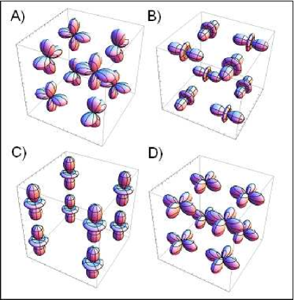
Figure 1: (Color online) Schematic view of four representative orbital configurations on a cubic cluster: (a) AO order with $\langle\tau^{a(b)}_{i}\rangle=1/2$ changing from site to site and $\langle\tau^{c}_{i}\rangle=-1/4$, obtained for $E_{z}<0$, (b) AO order with $\langle\tau^{a(b)}_{i}\rangle=-1/2$ changing from site to site and $\langle\tau^{c}_{i}\rangle=-1/4$, obtained for $E_{z}>0$, (c) FO order with occupied $z$ orbitals and $\langle\tau^{c}_{i}\rangle=-1/2$ (cigar-shaped orbitals), and (d) FO order with occupied $x$ orbitals and $\langle\tau^{c}_{i}\rangle=1/2$ (clover-shaped orbitals).

The bilayer spin-orbital $d^{9}$ model Eq. (7) poses a difficult many-body problem which cannot be solved exactly. The only simple limits are either $|E_{z}|\to\infty$ or $\eta\to(1/3)^{-}$ which we discuss below. In the first case the dominant term is the crystal field $\propto E_{z}$ and, depending on its sign, we get uniform orbital configuration $\tau^{c}_{i}\equiv\pm 1/2$ and $\tau^{a,b}_{i}\equiv\mp 1/4$. After inserting these classical expectation values into the Hamiltonian Eq. (7) we are left with the spin part which has purely Heisenberg form.

We will show below that in the bilayer geometry of the lattice the single-site MF approximation predicts long-range ordered $G$-AF phases at $\eta=0$ known from the 3D spin-orbital $d^{9}$ model,Fei97 see Fig. 2(d). For negative $E_{z}\to-\infty$ and FO order of $z$ orbitals shown in Fig. 1(c), we get an AF coupling in the $c$ direction and a weaker AF coupling in the $ab$ planar directions (in the regime of small $\eta$). For positive $E_{z}\to\infty$ one finds instead the FO order of $x$ orbitals shown in Fig. 1(d), and two $ab$ planes decouple, so we are left with the AF Heisenberg model on two independent 2D square lattices. In this case and the spins exhibit either $G$-AF, see Fig. 2(d) or $C$-AF order (not shown). Ferromagnetism is obtained in the present model for any $E_{z}$ if $\eta$ is sufficiently large, i.e., when the superexchange is dominated by terms proportional to $r_{1}$ which favor formation of spin triplets on the bonds accompanied by AO order depicted in Figs. 1(a) and 1(b).

In what follows we will show the simplest, single-site MF approximation of the Hamiltonian Eq. (7) and the resulting phase diagram. The Hamiltonian, originally expressed in terms of bond operators, can be then written in a ”single-site” form given below:

$${\cal H}_{\rm MF}\!\! = \!\frac{1}{2}J\sum_{i,\gamma}\!\left\{\tau^{\gamma}_{i}\tau^{\gamma}_{i+\gamma}(\chi^{\gamma}-\xi^{\gamma})+\frac{1}{2}\tau^{\gamma}_{i}\xi^{\gamma}-\frac{1}{4}(\chi^{\gamma}+\xi^{\gamma})\right\}$$ (12)

$$- E_{z}\sum_{i}\tau_{i}^{c},$$

with sum running over all sites and cubic axes $\gamma=a,b,c$. Here we adopted a shorthand notation with $i+\gamma$ meaning the nearest neighbor of site $i$ in the direction $\gamma$.

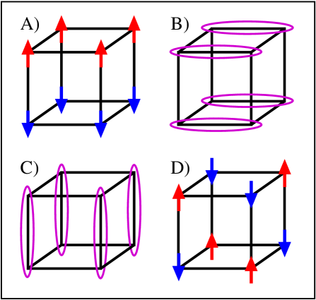
Figure 2: (Color online) Schematic view of four different spin ordered phases on a cube realized in the $d^{9}$ spin-orbital model Eq. (7): (a) $A$-AF configuration, (b) plaquette valence bond (PVB) singlet configuration, (c) VB$z$ phase with singlets along the $c$ axis, and (d) $G$-AF configuration. Arrows stand for up or down spins, oval (violet) frames indicate singlets. Spin disordered phases with singlets on certain bonds (b) and (c) are stabilized by particular orbital order, see Sec. III.

The quantities

$$\chi^{\gamma}=\left\{\begin{array}[]{ccc}r_{1}\Pi_{t}^{\gamma}+r_{2}\Pi_{s}^{\gamma}&if&\gamma=a,b\\ \frac{1}{2}(r_{1}\Pi_{t}^{\gamma}+r_{2}\Pi_{s}^{\gamma})&if&\gamma=c\end{array}\right\},$$ (15)

and

$$\xi^{\gamma}=\left\{\begin{array}[]{ccc}(r_{2}+r_{4})\Pi_{s}^{\gamma}&if&\gamma=a,b\\ \frac{1}{2}(r_{2}+r_{4})\Pi_{s}^{\gamma}&if&\gamma=c\end{array}\right\},$$ (16)

are parameters obtained by averaging over spin operators. The coefficients $1/2$ in the $\chi^{\gamma}$ and $\xi^{\gamma}$ terms along the $c$ axis follow from the bilayer geometry of the lattice. We assumed that the spin order, determining $\chi^{\gamma}$ and $\xi^{\gamma}$, depends only on the direction $\gamma$ and not on site $i$. This is sufficient to investigate the phases with either AF or FM long-range order. More precisely, these are spin-singlet and spin-triplet projectors $\Pi_{s(t)}^{\gamma}\equiv\Pi^{s(t)}_{i,i+\gamma}$ Eqs. (10) that are independent of $i$. As far as only a single site is concerned the spins cannot fluctuate at zero temperature and the projectors can be replaced by their average values:

$$\Pi_{s}^{\gamma}=\frac{1}{4}-\langle{\bf S}_{i}\cdot{\bf S}_{i+\gamma}\rangle,\hskip 14.22636pt\Pi_{t}^{\gamma}=\frac{3}{4}+\langle{\bf S}_{i}\cdot{\bf S}_{i+\gamma}\rangle.$$ (17)

The values of the projectors depend on the assumed spin order. Here we consider four different spin configurations: (i) $G$-AF - antiferromagnet in all three directions shown in Fig. 2(d), (ii) $C$-AF - antiferromagnet in the $ab$ planes with FM correlations in the $c$ direction (not shown), (iii) $A$-AF - AF phase with FM order in the $ab$ planes and AF correlations in the $c$ direction depicted in Fig. 2(a), (iv) FM phase (not shown). The numerical values of the spin projection operators in these phases are listed in Table 1.

Table 1: Mean values of triplet $\Pi_{t}^{\gamma}$ and singlet $\Pi_{s}^{\gamma}$ projection operators Eqs. (17) for a bond $\langle ij\rangle$ along the axis $\gamma$ in different phases with long-range magnetic order which occur in the MF phase diagram, see Fig. 3.

phase	$\Pi_{t}^{a(b)}$	$\Pi_{t}^{c}$	$\Pi_{s}^{a(b)}$	$\Pi_{s}^{c}$
$G$-AF	1/2	1/2	1/2	1/2
$C$-AF	1/2	1	1/2	0
$A$-AF	1	1/2	0	1/2
FM	1	1	0	0

After fixing spins, the MF approximation involves the well-know decoupling for the orbital operators:

$$\tau_{i}^{\gamma}\tau_{i+\gamma}^{\gamma}\simeq\langle\tau_{i}^{\gamma}\rangle\tau_{i+\gamma}^{\gamma}+\tau_{i}^{\gamma}\langle\tau_{i+\gamma}^{\gamma}\rangle-\langle\tau_{i}^{\gamma}\rangle\langle\tau_{i+\gamma}^{\gamma}\rangle.$$ (18)

The last step is to define sublattices for the orbitals. The most reasonable choice would be to assume AO order meaning that neighboring orbitals are always rotated by $\pi/2$ in the $ab$ plane with respect to each other. To implement this structure into the MF Hamiltonian we define new direction $\bar{\gamma}$ as follows: $\bar{\gamma}=b,a$ for $\gamma=a,b$ and $\bar{\gamma}=c$ for $\gamma=c$. Using $\bar{\gamma}$ we can now easily define staggered order parameters:

$$t_{i}^{\gamma}\equiv\langle\tau_{i}^{\gamma}\rangle=\langle\tau_{i\pm\gamma}^{\bar{\gamma}}\rangle.$$ (19)

The final single-site MF Hamiltonian can be written in the same form for any site so further on we will not use site index $i$ anymore. The desired formula is:

$${\cal H}^{(0)}_{{\rm MF}}=\sum_{\gamma}\Theta^{\gamma}\tau^{\gamma}+f(t_{a},t_{c})=\alpha\sigma^{z}+\beta\sigma^{x}+f(t_{a},t_{c}),$$ (20)

with

$$\Theta^{\gamma}=\frac{1}{2}\xi^{\gamma}+t^{\bar{\gamma}}(\chi^{\gamma}-\xi^{\gamma})-E_{z}\delta_{\gamma c},$$ (21)

and

$$f(t_{a},t_{c})=-\frac{1}{8}\sum_{\gamma}\left\{(\chi^{\gamma}+\xi^{\gamma})+4t^{\gamma}t^{\bar{\gamma}}(\chi^{\gamma}-\xi^{\gamma})\right\}.$$ (22)

For convenience we set $J=1$; note that the energy scale can easily be recovered by replacing $E_{z}$ by $E_{z}/J$. As we can see the MF Hamiltonian is very simple and can be written in terms of two Pauli matrices $\{\sigma^{x},\sigma^{z}\}$ with

$$\alpha=\frac{1}{2}\left(\Theta^{c}-\frac{1}{2}\Theta^{a}-\frac{1}{2}\Theta^{b}\right),\hskip 14.22636pt\beta=\frac{\sqrt{3}}{4}\left(\Theta^{a}-\Theta^{b}\right).$$ (23)

Solving the $2\times 2$ eigen-problem we obtain self-consistency equations for the order parameters $t^{a}$ and $t^{c}$:

$$t^{a} = \frac{1}{4\Delta}\left(\alpha-\sqrt{3}\beta\right),$$ (24)

$$t^{c} = -\frac{1}{2\Delta}\alpha,$$ (25)

where $\Delta=\sqrt{\alpha^{2}+\beta^{2}}$ and the ground state energy given by:

$$E_{0}=-\Delta-f(t^{a},t^{c}).$$ (26)

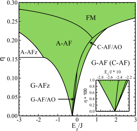
Figure 3: (Color online) Phase diagram of the bilayer $d^{9}$ spin-orbital model Eq. (20) obtained in the single-site MF approximation with spin and orbital MFs. In this approach the $G$-AF and $C$-AF phases (for $E_{z}>-0.25$ and moderate $\eta$) have exactly the same energy. Shaded gray (green) area indicates phases with AO order, while the remaining states with long-range $G$-AF spin order are accompanied by FO order. The enlarged area around the multicritical point at $E_{z}=-0.25J$ and $\eta=0$ is shown in the inset.

The solution of self-consistency equations is very elegant and entertaining so we are not going to present it here and recommend it to the reader as an exercise (the results can be next compared with those given in the Appendix). It turns out that all four phases considered here can appear as orbitally uniform, i.e., having FO order with orbitals being either perfect clovers or perfect cigars everywhere, or as phases with AO order between two sublattices. The phase diagram presented in Fig. 3 was obtained by purely energetic consideration and shows the boarder lines between phases with the lowest energies for given $\eta$ and $E_{z}$. This diagram is surprisingly complex taking into account the simplicity of the single-site approach; it reveals seven different phases. For $\eta=0$ we have only two AF phases: (i) $G$-AF$z$ for $E_{z}<-1/4J$ and (ii) $G$-AF for $E_{z}>-1/4J$, with a different but uniform orbital configuration (FO order) which involves either cigar-shaped $z$ orbitals in the $G$-AF$z$ phase, see Fig. 1(c), or clover-shaped $x$ orbitals in the $G$-AF, see Fig. 1(d). Because of the planar orbital configuration in the latter $G$-AF phase one finds no interplane exchange coupling and thus this phase is degenerate with the $C$-AF one.

For higher $\eta$ the number of phases increases abruptly by three phases with AO configurations, as shown in the inset of Fig. 3: the $A$-AF, $G$-AF/AO and $C$-AF/AO phase. Surprisingly, the AO version of the $G$-AF phase is connected neither to $z$ nor to $x$ FO order in an antiferromagnet, excluding the multicritical point at $(E_{z}/J,\eta)=(-0.25,0)$, and disappears completely for $\eta\approx 0.118$. The $C$-AF/AO phase stays on top of uniform $G$($C$)-AF phase, lifting the degeneracy of the above phases at relatively large $\eta$ and then gets replaced by the FM phase which always coexists with AO order. One can therefore conclude that the $G$($C$)-AF degeneracy is most easily lifted by turning on the orbital alternation.

On the opposite side of the diagram the $G$-AF$z$ phase is completely surrounded by $A$-AF phases: for $\eta>(2/\sqrt{3}-1)$ the $G$-AF$z$ phase turns into orbitally uniform $A$-AF$z$ independently of the value of $E_{z}$ (interorbital triplet excitations dominate then on the bonds in the $ab$ planes), and for smaller $\eta$ into the $A$-AF phase with AO order. In the $A$-AF phase the AF correlations in the $c$ direction survive despite the overall FM tendency when $\eta$ grows. This follows from the orbitals’ elongation in the $c$ direction present for $E_{z}<0$, which would cause interplane singlets formation if we were not working in single-site MF approximation, see Sec. III. In the present case it favors either the $G$-AF$z$ or $A$-AF($z$) configuration with uniform or alternating orbitals depending on the values of $E_{z}/J$ and $\eta$. Finally, the FM phase is favorable for any $E_{z}$ if only $\eta$ is sufficiently close to $1/3$ which only confirms that the single-site MF approximation is sound and not totally wrong with this respect.

The central part of the presented diagram is the most frustrated one judging by the number of competing phases with long-range spin order. This behavior is consistent with that found in the 3D spin-orbital $d^{9}$ model in the regime of $E_{z}\simeq 0$ and finite $\eta$.Fei97 Four of these phases could be expected by looking at the phase diagram of the 3D model: two $G$-AF phases, the $A$-AF phase and the FM phase.Fei97 Note, however, that in the phases stable in the central part of the phase diagram, namely in the $A$-AF, $A$-AF/AO and FM phase, the occupied orbitals alternate. While the FM phase is not surprising in this respect and obeys the Goodenough-Kanamori rule of having FM spin order accompanied by the AO order, in the $A$-AF one finds an example that both spin and orbital order could in principle alternate between the two $ab$ planes. This finding suggests that in this central part of the phase diagram one may expect either other VB-type phases or even states with more complex spin-orbital disorder. Such ordered or disordered phases require a more sophisticated approach, either variational wave functions,Fei97 ; Nor08 or the embedded cluster approach which we explain below in Sec. II.3

II.3 Cluster mean–field Hamiltonian

Now we introduce a more sophisticated approach which goes beyond the single-site MF approximation of Sec. II.2. In what follows we use a cluster MF approach with a cube depicted in Fig. 4. It contains eight sites coupled to its neighbors along the bonds in $ab$ planes by the MF terms. This choice is motivated by the form of the Hamiltonian with different interactions along the bonds in three different directions — the cube is the smallest cluster which does not break the symmetry between the $a$ and $b$ axes and contains equal numbers of $a$, $b$ and $c$ bonds. After dividing the entire bilayer square lattice into identical cubes which cover the lattice, the Hamiltonian (7) can be written in a cluster MF form as follows,

$${\cal H}_{\rm MF}=\sum_{m\in{\cal C}}({\cal H}^{\rm int}_{m}+{\cal H}^{\rm ext}_{m})\,,$$ (27)

where the sum runs over the set of cubes ${\cal C}$, with individual cube labeled by $C_{m}\in{\cal C}$. Here ${\cal H}^{\rm int}_{m}$ contains all bonds from ${\cal H}_{m}$ belonging to the cube $C_{m}$ and the crystal field terms $\propto E_{z}$, i.e., it depends only on the operators on the sites inside the cube, while ${\cal H}^{\rm ext}_{m}$ contains all bonds outgoing from the cube $m$ and connecting neighboring clusters, making them correlated.

The basic idea of the cluster MF approach is to approximate ${\cal H}^{\rm ext}_{m}$ by $\tilde{{\cal H}}^{\rm ext}_{m}$ containing only operators from the cube $m$. This can be accomplished in many different ways depending on which phase we wish to investigate. Our choice will be to take $\tilde{{\cal H}}^{\rm ext}_{m}$ of the following form:

$$\tilde{{\cal H}}^{\rm ext}_{m}=\frac{1}{2}\!\sum_{\gamma=a,b\atop i\in C_{m}}\left\{S^{z}_{i}a^{\gamma}_{i}+S^{z}_{i}\tau^{\gamma}_{i}b^{\gamma}_{i}+\tau^{\gamma}_{i}c^{\gamma}_{i}+d^{\gamma}_{i}\right\},$$ (28)

containing spin field $S^{z}_{i}$ breaking SU(2) symmetry, orbital field $\tau^{\gamma}_{i}$ and spin–orbital field $S^{z}_{i}\tau^{\gamma}_{i}$. Coefficients $\{a^{\gamma}_{j},b^{\gamma}_{j},c^{\gamma}_{j},d^{\gamma}_{j}\}$ are the Weiss fields and should be fixed self–consistently depending on $E_{z}$ and $\eta$. Our motivation for such expression is simple: if orbital degrees of freedom are fixed then the problem reduces to the Heisenberg model which has long–range ordered AF phase — that is why we take $S^{z}_{i}$ field, the orbitals are present in the Hamiltonian so taking $\tau^{\gamma}_{i}$ is the simplest way of treating them on equal footing to describe possible orbital order. Finally, we introduce also spin-orbital field $S^{z}_{j}\tau^{\gamma}_{j}$ because we believe that in some phases spins and orbitals alone do not suffice to describe the symmetry breaking and these operators can act together.

Figure 4: Schematic view of the cluster used in the Bethe–Peierls–Weiss MF approach of Sec. II.3. Vertices $i=1,\cdots,8$ and directions $\gamma=a,b,c$ are marked in the figure, and dashed lines stand for the outgoing MF interactions in the $a$ and $b$ direction.

The standard way to go on is to write self–consistency equations for the Weiss fields. This can be done in a straightforward fashion: we take the operator products from ${\cal H}^{\rm ext}_{m}$ and divide them into a part depending only on $O_{i}$ operators from the cube $m$, and on $O_{j}$ ones — from a neighboring cube $n$. Then we use the well known MF decoupling for such operator products,

$$O_{i}O_{j} \approx \langle O_{i}\rangle O_{j}+O_{i}\langle O_{j}\rangle-\langle O_{i}\rangle\langle O_{j}\rangle$$

$$= O_{i}\langle O_{j}\rangle-\frac{1}{2}\langle O_{i}\rangle\langle O_{j}\rangle+O_{j}\langle O_{i}\rangle-\frac{1}{2}\langle O_{i}\rangle\langle O_{j}\rangle\,,$$

and write it in a symmetric way. Now the first two terms can be included into $\tilde{{\cal H}}^{\rm ext}_{m}$ and the last two into $\tilde{{\cal H}}^{\rm ext}_{n}$. This procedure can be applied to all operator products in ${\cal H}^{\rm ext}_{m}$ and full $\tilde{{\cal H}}^{\rm ext}_{m}$ can be recovered in the form given by Eq. (28). Repeating this for all clusters leads to a Hamiltonian describing a set of commuting cubes interacting in a self–consistent way. After using Eq. (LABEL:deco) on the Hamiltonian Eq. (7) we obtain the formulas for the Weiss fields:

$$a^{\gamma}_{i} = \frac{1}{2}(r_{2}+r_{4})u^{\gamma}_{i}+\frac{1}{4}(r_{2}-r_{1})s^{\gamma}_{i},$$ (30)

$$b^{\gamma}_{i} = -(r_{4}+r_{1})u^{\gamma}_{i}-\frac{1}{2}(r_{2}-r_{1})s^{\gamma}_{i},$$ (31)

$$c^{\gamma}_{i} = \frac{1}{4}(3r_{1}-r_{4})t^{\gamma}_{i}+\frac{1}{8}(r_{2}+r_{4}),$$ (32)

$$d^{\gamma}_{i} = -\frac{1}{2}(r_{1}+r_{4})u^{\gamma}_{i}u^{\gamma}_{m,i}-\frac{1}{4}(r_{2}-r_{1})(s_{i}u^{\gamma}_{i}+s^{\gamma}_{i}u^{\gamma}_{m,i})$$ (33)

$$- \frac{1}{16}(r_{2}+r_{4})(t^{\gamma}_{m,i}-t^{\gamma}_{i})+\frac{1}{8}(r_{4}-3r_{1})t^{\gamma}_{i}t^{\gamma}_{m,i}$$

$$- \frac{1}{32}(3r_{1}+2r_{2}+r_{4}),$$

where the order parameters at site $i$ are:

$$s_{i} \equiv \left\langle S^{z}_{i}\right\rangle,$$ (34)

$$t^{\gamma}_{m,i} \equiv \left\langle\tau^{\gamma}_{i}\right\rangle,$$ (35)

$$u^{\gamma}_{m,i} \equiv \left\langle S^{z}_{i}\left(\frac{1}{2}-\tau^{\gamma}_{i}\right)\right\rangle.$$ (36)

Note that $\{s_{i},t^{\gamma}_{m,i},u^{\gamma}_{m,i}\}$ are the mean values of operators at site $i$ belonging to the cluster $m$, and $\{s^{\gamma}_{i},t^{\gamma}_{i},u^{\gamma}_{i}\}$ are the mean values of the same operators at sites neighboring with $i$ in the direction $\gamma$. The geometry of a bilayer implies that each site $i$ has one neighbor along the axis $a$ and another one along the axis $b$, and these sites belong to different cubes.

The next crucial step is to impose a condition that $\{s^{\gamma}_{i},t^{\gamma}_{i},u^{\gamma}_{i}\}$ are related to the order parameters obtained on the internal sites of the considered cluster. The simplest solution is to assume that all clusters have identical orbital configuration; $t^{\gamma}_{i}=t^{\gamma}_{m,i}$, spin configuration is in agreement with a type of global magnetic order we want to impose; $s^{\gamma}_{i}=\pm s_{i}$ and spin orbital configuration is as if spin and orbitals were factorized, i.e., $u^{\gamma}_{i}=\pm u^{\gamma}_{m,i}$. This solution has one disadvantage: if $a$ or $b$ direction is favored in the orbital configuration of the cube then this broken symmetry will propagate through whole lattice which is contradictory with the form of the Hamiltonian Eq. (7). That is why it is better to assume that two neighboring cubes can differ in orbital (and spin-orbital) configuration by the interchange of $a$ and $b$ direction, i.e.,

$$s^{\gamma}_{i}=\pm s_{i},\hskip 19.91684ptt^{\gamma}_{i}=t^{\bar{\gamma}}_{m,i},\hskip 19.91684ptu^{\gamma}_{i}=\pm u^{\bar{\gamma}}_{m,i}$$ (37)

with $\bar{\gamma}$ being the complementary direction in the $ab$ plane to $\gamma$, i.e., $(\gamma,\bar{\gamma})=(a,b),(b,a)$. This relation gives the same results as the previous one in case when the $(a,b)$ symmetry in the cube is not broken, but keeps the whole system $(a,b)$ symmetric in the other case. Here we again treat the spin-orbital field as factorized but surprisingly it turns out that this does not prevent spin-orbital entanglement to occur, see below. We have also tried to impose relations between $u^{\gamma}_{i}$ and $u^{\gamma}_{m,i}$ which have nothing to do with spin and orbital sectors alone but this only resulted in the lack of convergence of self–consistency iterations.

II.4 Self–consistent iterative procedure

The self–consistency equations cannot be solved exactly because the effective cluster Hilbert space is too large even if we use total ${\cal S}^{z}$ conservation in the considered cluster $m$ (then the largest subspace dimension is $d=17920$) and because of their non–linearity. The way out is to use Bethe–Peierls–Weiss method, i.e., set certain initial values for the order parameters $\{s_{i},t^{\gamma}_{m,i},u^{\gamma}_{m,i}\}$ and next employ Lanczos algorithm to diagonalize ${\cal H}_{\rm MF}$ Eq. (27). Below we present results obtained by self-consistent calculations of phases with broken symmetry or with spin disorder. In order to determine the ground state one recalculates mean values of spin, orbital and spin-orbital fields given by Eqs. (37) and determines new order parameters. This procedure is continued until convergence (of energy and order parameters) is reached. This process can be very slow due to the number of order parameters which is $24$ (three per site) for the cube but we have overcome this problem by imposing certain symmetry breaking on the cluster. We implement it in the following way: after each iteration we calculate $\{s_{i},t^{\gamma}_{m,i},u^{\gamma}_{m,i}\}$ only for one site $i=1$ and the remaining coefficients are fixed assuming certain symmetries of the phase we are searching for.

For simplicity let us enumerate the vertices $i=1,\cdots,8$ in the cubic cluster as shown in Fig. 4. To obtain $G$-AF phases we assume that:

$$s_{i}=\left\{\begin{array}[]{c}s_{1}\;\;\;if\;\;\;i\in A\\ -s_{1}\;\;if\;\;i\in B\end{array}\right\}$$ (40)

for a two-sublattice structure, where $A=\{1,4,5,8\}$ and $B=\{2,3,6,7\}$. In FM case it is enough to put $s_{i}\equiv s_{1}$ and in case of FM order within the planes and AF between them (in the $A$-AF phase) we use instead: $s_{i}=(-1)^{i-1}s_{1}$. In the orbital sector we can impose a completely uniform configuration with $t^{\gamma}_{m,i}\equiv t^{\gamma}_{m,1}$, which can however lead to non–uniform configuration of the whole system because neighboring clusters are rotated by $\pi/2$ with respect to each other, or we can produce a phase with AO order taking:

$$t^{\gamma}_{m,i}=\left\{\begin{array}[]{c}t^{\gamma}_{m,1}\;\;\;if\;\;i\in A\\ t^{\bar{\gamma}}_{m,1}\;\;if\;\;i\in B\end{array}\right\}$$ (43)

with $(\gamma,\bar{\gamma})=(a,b),(b,a)$. Other choices would be to take the above equation either with $A=\{1,2,5,6\}$ and $B=\{3,4,7,8\}$ or with $A=\{1,3,5,7\}$ and $B=\{2,4,6,8\}$. More generally speaking, every choice of orbital sublattices is good as long as the total MF wave function does not violate the symmetry between directions $a$ and $b$. The sublattices for spin-orbital field are constructed as if $u^{\gamma}_{m,1}$ could be expressed as $u^{\gamma}_{m,i}=s_{i}(\frac{1}{2}-t^{\gamma}_{m,i})$.

III Phase diagrams

III.1 Disentangled spin and orbital operators

The zero–temperature phase diagram of the present bilayer $d^{9}$ spin-orbital model Eq. (7) depends on parameters $(E_{z},\eta)$, and was obtained by comparing ground state energies for different sublattices formed by $\{s_{i},t^{\gamma}_{m,i},u^{\gamma}_{m,i}\}$ MFs. In this way we determined the ground state with the lowest energy and its order parameters. We begin with the phase diagram of Fig. 5 obtained by assuming that spin-orbital operators may be factorized into spin and orbital parts, i.e., $u^{\gamma}_{m,i}\equiv s_{i}(1/2-t^{\gamma}_{m,i})$ or:

$$\langle S^{z}_{i}\tau^{\gamma}_{i}\rangle\equiv\langle S^{z}_{i}\rangle\langle\tau^{\gamma}_{i}\rangle.$$ (44)

Next we report the phase diagram (in Sec. III.2), where we include $u^{\gamma}_{m,i}$ calculated following the definition in Eq. (36). Comparing these two schemes allows us to determine which phases cannot exist without spin-orbital entanglement.

The low–$\eta$ part of the diagram in Fig. 5 is dominated by three phases: VB$z$ for negative $E_{z}$, PVB for $E_{z}$ close to zero and $G$-AF for positive $E_{z}$. The VB$z$ phase with ordered interlayer valence bonds for occupied $z$ orbitals and spin singlets, see Fig. 2(c), has replaced the $G$-AFz phase obtained before in Sec. II.2. Both phases exhibit uniform FO order, i.e., $t^{c}_{m,i}$ is close to $-1/2$ for all $i$ which means that orbitals take the shape of cigars aligned along the $c$ bonds, see Fig. 1(c). One finds that quantum fluctuations which could be included within the present approach select the VB$z$ phase and magnetization vanishes due to the singlets formation. For higher values of $E_{z}\simeq 0$ also a different phase is found: the plaquette VB (PVB) phase with singlets formed on the bonds in $a$ or $b$ direction of the cluster, see Fig. 2(b). This phase breaks the $a$–$b$ symmetry of the model locally but the global symmetry is preserved thanks to the $\pi/2$ rotation of neighboring clusters (see Eq. (37)). The orbitals are again uniform within the cluster with $t^{a}_{m,i}$ or $t^{b}_{m,i}$ close to $-1/2$, meaning that they take shape of cigars pointing in the direction of the singlets. For high positive values of $E_{z}$ the ground state is the $G$-AF phase with long–range AF order and FO order of $x$ occupied orbitals, i.e., $t^{c}_{m,i}$ close to $1/2$, see Fig. 1(d). This means that orbitals are indeed of the $x$ type and take shape of four–leaf clovers in the $ab$ plane with lobes pointing along $a$ and $b$ directions which makes the two planes very weakly coupled.

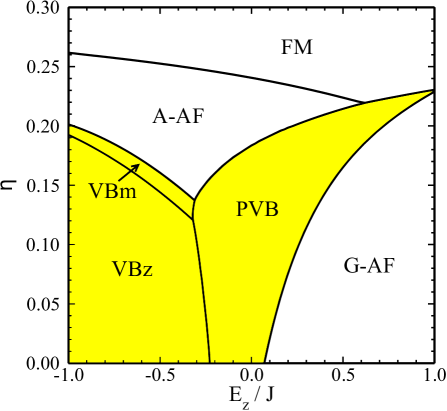
Figure 5: (Color online) Phase diagram of the $d^{9}$ spin-orbital superexchange model Eq. (27) obtained using the cluster method for an embedded cube with factorized spin-orbital operators. Valence-bond phases with spin disorder are stable in the shaded area.

The FO order in the VB$z$ and $G$-AF phases agrees with the limiting configurations for $E_{z}\to\pm\infty$ described earlier. The first of them is a quantum phase with local singlets, in contrast to the $G$-AF$z$ one found already in Sec. II.2 and in the 3D spin-orbital $d^{9}$ model.Fei97 If we consider now the VB$z$ phase and increase $\eta$, we pass through the VBm phase (where ”m” stands for mixed orbital configuration) and reach the $A$-AF phase with non–zero global magnetization such that spins order ferromagnetically in the $ab$ planes and antiferromagnetically between them (along $c$ axis), see Fig. 2(a). We believe that this regime of the phase diagram is of relevance for the spin and orbital correlations in K₃Cu₂F₇ and discuss it also in Sec. VII. The orbital order is of the AO type with $t^{c}_{m,i}$ close to zero, positive or negative depending on $E_{z}$, see Figs. 1(a) and 1(b). The VBm phase occurs when the orbitals in the VB$z$ phase start to deviate from the uniform configuration and ends when the global magnetization appears, accompanied by the change of the orbital order. The first transition is of second order, being the only second order phase transition in this diagram of Fig. 5.

The presence of both $A$-AF phases on top of the VB$z$ can be understood qualitatively as follows: in the VB$z$ phase AF spin coupling is strong only within the singlets, so if $\eta$ is increased the weak in-plane spin correlations can easily switch to FM ones, while AF correlations will still survive between the planes. The last phase of the diagram is the FM phase with AO order, similar to the AO order in the $A$-AF phase. Due to the absence of thermal and quantum fluctuations the magnetization in this phase is constant and maximal. The FM phase appears for any $E_{z}$, if only $\eta$ is sufficiently close to $1/3$, which agrees qualitatively with the previous discussion of the exact limiting configurations and with the phase diagram found before in the single-site MF approach, see Fig. 3.

Comparing Fig. 5 to the MF phase diagram of Fig. 3 we can immediately recognize the main difference: the existence of the VB$z$ and PVB phases. These phases contain spin singlets on the bonds and do not follow from the single-site MF approach. Another difference is the lack of sharp transitions between AO and FO order within one phase; these transitions are smoothened by spin fluctuations absent in the single-site MF and perfect FO configurations are now available only for extremely high values of $|E_{z}|$.

III.2 Phase diagram with spin-orbital field

When the spin-orbital MF is not factorized but calculated according to its definition given in Eq. (36), one finds the phase diagram displayed in Fig. 6. We would like to emphasize that this non-factorizability cannot be included within the single-site MF approach because there all spin fluctuations are absent. Of course, one can imagine that we take the $S^{z}_{i}\langle S^{z}_{i+\gamma}\rangle$ decoupling in the pure-spin sector and $S^{x}_{i}\langle S^{x}_{i+\gamma}\rangle$ decoupling in the spin-orbital sector of the Hamiltonian Eq. (7) leading to the fluctuating spins but this would break both the magnetization conservation and homogeneity of the spin-spin interactions included into the Kugel-Khomskii model.

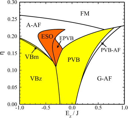
Figure 6: (Color online) The phase diagram of the cluster MF Hamiltonian Eq. (27) of the $d^{9}$ spin-orbital model for a bilayer, with independent spin, orbital and spin-orbital mean fields. Valence-bond phases with spin disorder are stable in the light shaded (yellow) area, and phases with spin-orbital entanglement are indicated by dark gray (orange) shading.

In addition to the phases obtained in the phase diagram of Fig. 5, we get here also the following phases: ESO, EPVB and PVB-AF (the VBm phase is still stable between the VB$z$ and $A$-AF ones but has much smaller area). The first two above phases are formed in the highly frustrated region of the phase diagram where both $E_{z}$ and $\eta$ are moderate. ESO stands for entangled spin–orbital phase and is characterized by relatively high values of spin-orbital order parameters, especially for high $\eta$ values when other order parameters are close to zero. This phase contains singlets along the bonds parallel to the $c$ axis, its magnetization vanishes and the orbital configuration is uniform. One can say that this is the VB$z$ phase with weakened orbital order transformed into uniform spin-orbital order for the same spin and orbital sublattices. EPVB stands for entangled PVB phase and resembles it, but has in addition finite non–uniform spin-orbital fields, and weak global AF order. A different type of phase with spin-orbital entanglement is the PVB-AF phase connecting PVB and $G$-AF in a smooth (as it will be shown below) way but only if $\eta$ is large enough. In contrast to the direct PVB-to-$G$-AF transition, passing through the PVB-AF involves second order phase transitions and the same happens in case of the EPVB connecting the ESO and PVB phases. Similarly to the previous diagram, the transition from the VB$z$ to VBm phase is of the second order while the other transitions produce discontinuities in order parameters (see Sec. IV) and correlation functions (see Sec. V).

Finally, we should also point out that the $G$-AF/$C$-AF degeneracy found in Fig. 3 is lifted in the cluster approach and the $C$-AF phase does not appear in any of the two phase diagrams presented in Figs. 5 and 6. Another interesting feature of the phase diagrams are points of high degeneracy where different phases have the same ground-state energies. In case of the single-site MF diagram this quantum critical point is found at $(E_{z}=-1/4J,\eta=0)$, where six phases meet. The use of cluster MF method which includes singlet phases lifts this point upwards along the border line between VB$z$ and PVB to $(E_{z},\eta)\approx(-0.3J,0.11)$ in case of Fig. 6. This means that singlet formation acts against interaction frustration caused by Hund’s exchange coupling and moves the most frustrated region of phase diagram to high-$\eta$ regime. This shows once again that the simple single-site approach is not sufficient to describe correctly the properties of the bilayer $d^{9}$ spin-orbital model.

IV The order parameters

The ground state is characterized by order parameters obtained directly during the self–consistency iterations in each phase: spin, orbital and spin-orbital order parameters, $\{s_{1},t^{a,b}_{m,1},u^{a,b}_{m,1}\}$. We focus here on the phases shown in the phase diagram of Fig. 6. For the physical reasons it is however better justified to define joint spin-orbital order parameter in a slightly different way, introducing a new variable $v^{\gamma}_{m,i}$ as follows:

$$v^{\gamma}_{m,i}\equiv\langle S^{z}_{i}\tau^{\gamma}_{i}\rangle,$$ (45)

which differs from the old order parameter by a subtraction of the spin field, i.e., $u^{\gamma}_{m,i}=\frac{1}{2}s_{i}-v^{\gamma}_{m,i}$. Now one can study the behavior of order parameters along different cuts of the phase diagram of Fig. 6 and determine types of phase transitions. Below we present a few representative results. For this purpose we first choose $\eta=0.05$ and start within the VB$z$ phase, where by increasing $E_{z}$ one gets first into the PVB and next to $G$-AF phase, see Fig. 7. For $\eta=0.15$ there are even more phases and one passes through the $A$-AF, ESO, EPVB, PVB, and AF-PVB phases, before reaching finally the $G$-AF phase, see Figs. 8 and 9. We also investigated the dependence of order parameters on Hund’s exchange coupling — we fixed $E_{z}=-0.72J$, started in the VB$z$ phase and increased $\eta$ to get to the VBm and $A$-AF phases — these results are shown in Figs. 10.

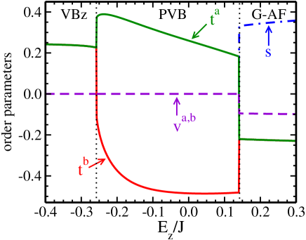
Figure 7: (Color online) Order parameters $\{s,t^{a,b},v^{a,b}\}$ for $\eta=0.05$ and $-0.4<E_{z}/J<0.3$ in the VB$z$, PVB and $G$-AF phase, from left to right.

In what follows we use shorthand notation for the order parameters,

$$\{s,t^{a,b},v^{a,b}\}\equiv\{s_{1},t^{a,b}_{m,1},v^{a,b}_{m,1}\}.$$ (46)

In Fig. 7 we displayed the order parameters for increasing $E_{z}$ in phases VB$z$, PVB and $G$-AF (separated by dotted lines in the plot). The sublattice magnetization $s$ is non–zero only in the $G$-AF phase because the remaining phases are of the VB crystal type, with spin singlets oriented either along the $c$ direction or in the $ab$ planes. In the $G$-AF phase the spin order grows stronger for increasing $E_{z}$ when the orbital fluctuations weaken and spin fluctuations present in the $G$-AF phase reduce $s$ from the classical value of 1/2.

Consider now decreasing values of $E_{z}$ in Fig. 7. Both orbital order parameters remain equal and close to $-1/4$ in the $G$-AF phase until the (first order) transition point to the PVB phase, where orbital configuration changes abruptly and becomes anisotropic. In this case the $a$–$b$ symmetry was broken in such a way that that spin singlets point in the PVB phase in $b$ direction and so the directional orbitals (cigars) do. This explains the robust orbital order with $t^{b}$ being close to $-1/2$ in most of the PVB phase. The global symmetry is not broken as the VB singlets form here a checkerboard pattern in the $ab$ plane, with AO order of directional orbitals along the $a$ and $b$ axis in the neighboring plaquettes. The transition to the VB$z$ phase is discontinuous (first order) in the orbital sector too: $t^{a}$ grows constantly while decreasing $E_{z}$ down to $0.4J$, drops slightly close to the transition point and jumps to $1/4$ in the VB$z$ phase, $t^{b}$ grows quickly to $t^{b}\approx 0.125$ while approaching the transition and then jumps to the value of $t^{a}$. Qualitatively this means that close to the above transition the orbital cigars pointing along the $b$ axis change gradually into a shape very similar to clover orbitals lying in the $bc$ plane and then suddenly the lobes along the $b$ direction disappear and we are left with the pure VB$z$ phase.

The spin-orbital order parameter behaves in a much less intriguing way; it remains zero in the VB$z$ and PVB phases, jumps to finite value at the PVB-to-$G$-AF transition and remains almost constant and close to $-0.1$ in the $G$-AF phase. The vanishing value of $v^{a,b}$ in the singlet phases is simple to understand: the orbitals are here fixed and spins form singlets and fluctuate independently between the values $\pm 1/2$. This means that $t^{a,b}$ and $s$ are not ”synchronized” in any way and only this could lead to $v^{a,b}\not=0$. This condition is satisfied in the $G$-AF phase; orbitals are fixed and the spin configuration is here determined by $s$ order parameter.

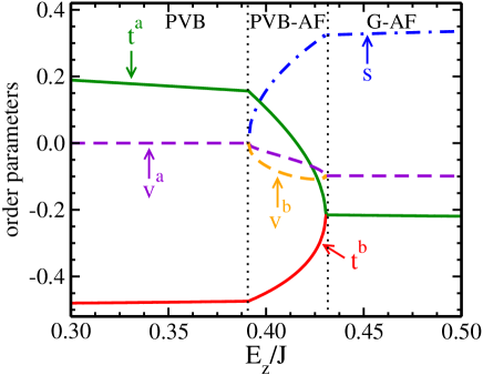
Figure 8: (Color online) Order parameters $\{s,t^{a,b},v^{a,b}\}$ for $\eta=0.15$ and $0.3<E_{z}/J<0.5$ in the PVB, PVB-AF and $G$-AF phase, from left to right.

Figure 8 shows that the transition between the PVB and $G$-AF phases can have a completely different character than described above. The difference comes from a higher value of $\eta$ which is now equal to $0.15$, enhancing the FM channel of superexchange and leading to the intermediate PVB-AF phase and to a smooth transition from the PVB to $G$-AF phase. In the PVB-AF phase staggered magnetization $s$ grows continuously from zero (in the PVB) to a finite value in the $G$-AF phase and remains saturated there. This means that planar singlets in the PVB phase decay gradually and spins get partially ”synchronized” with orbitals, moving toward uniform configuration which gives finite spin-orbital order parameters $v^{\gamma}\neq 0$. The anisotropy $(v^{a}\neq v^{b})$ follows from the anisotropy of orbitals inherited from the PVB order. This mechanism of the PVB-to-$G$-AF transition is absent for low values of $\eta$ — we anticipate that the enhanced FM component of interactions reduces spin fluctuations which makes the correlations between spins and orbitals possible.

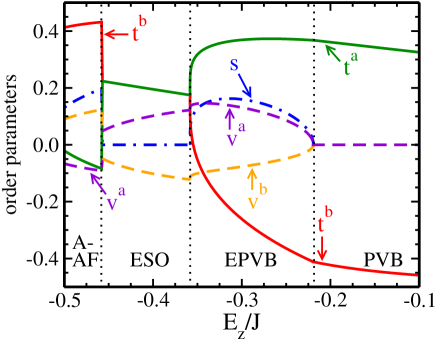
Figure 9: (Color online) Order parameters $\{s,t^{a,b},v^{a,b}\}$ for $\eta=0.15$ and $-0.5<E_{z}/J<-0.1$ in the $A$-AF, ESO, EPVB and PVB phases, from left to right.

In Fig. 9 we focus on the complementary regime of the phase diagram, $\eta=0.15$ and negative $E_{z}$. In this regime we describe three different consecutive phase transitions between the phases: $A$-AF, ESO, EPVB and PVB. The first phase transition can be regarded as a little bit artificial because this is a meeting point of two completely different types of spin and orbital order, with different symmetries and sublattices. For this reason the transition has to be discontinuous and the spin order parameter has different physical meaning on both sides of the transition line, i.e., $s$ in the magnetic moment in the $A$-AF phase while it is a weak AF order parameter in the ESO phase. We anticipate that a smooth crossover occurs in place of such a transition in the thermodynamic limit, nevertheless by comparing the energies we concluded that this transition follows from the cluster MF approach. Note also that the ESO phase has predominantly $z$ orbitals accompanied by fluctuations, i.e., $t^{c}\simeq-0.4$ and $t^{a}=t^{b}$, and may be seen as an extension of the VB$z$ phase.

On the contrary, the second quantum EPVB phase which occurs in the phase diagram of Fig. 6 may be seen as a precursor of the PVB phase and is characterized again by finite joint spin-orbital fluctuations, with $v^{\alpha}\neq 0$ for $\alpha=a,b$. What is especially peculiar in the EPVB phase is the non–zero staggered magnetization $s$ which grows smoothly from the zero values at the phase borders meaning that we have a wedge of antiferromagnetism between two VB configurations. The EPVB phase seems to be similar to PVB-AF in a sense that spin-orbital fields are non–zero and non–uniform but the qualitative behavior of the order parameters is different, e.g. in the EPVB phase spin-orbital fields have always opposite signs, while in the PVB-AF phase the sings are the same.

Looking at the orbital order parameters $t^{a,b}$ in the $A$-AF phase (Fig. 9), one observes similar anisotropy as in the PVB one but this time $a$-$b$ symmetry is not broken within the cluster because in the $A$-AF phase every orbital is rotated by $\pi/2$ with respect to its neighbors in the $ab$ plane. Another difference is that the orbitals take the shape of clovers, not cigars, with symmetry axes pointing along the $a$ or $b$ axis which is described by $t^{b}$ being close to $1/2$. In the $A$-AF phase we have also long–range magnetic order and finite spin-orbital fields, indicating joint behavior of spin and orbital MF variables.

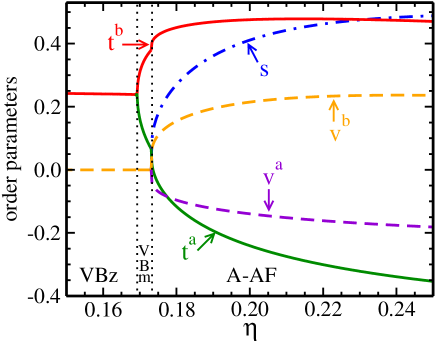
Figure 10: (Color online) Order parameters $\{s,t^{a,b},v^{a,b}\}$ for $E_{z}=-0.72J$ and $0.15<E_{z}/J<0.25$ in the VB$z$, VBm and $A$-AF phases, from left to right.

Next Fig. 10 shows the behavior of order parameters for $E_{z}=-0.72J$ and $\eta$ changing in an interval allowing us to study the transitions from the VB$z$ to VBm phase, and between the VBm and $A$-AF phase. In this case all the phases can be described by the same spin and orbital sublattices because VB$z$ is uniform in the orbital sector and has no long–range magnetic order so it can be described both in terms of the PVB and $A$-AF type of ordering. Global magnetization appears only in the $A$-AF phase jumping from the zero value in the VBm and growing with increasing $\eta$. Transition from the VB$z$ to VBm phase is continuous in both spin and orbital sectors.

The orbital order parameters $t^{a,b}$ bifurcate in Fig. 10 at $\eta\simeq 0.169$ from the isotropic value $t^{a}=t^{b}\simeq 1/4$ and the orbital anisotropy grows in the VBm phase to give AO order in the $A$-AF phase (Fig. 10), and next shows a discontinuity at the second transition. The final AO order can be described by clover orbitals with symmetry axes alternating between $a$ and $b$ directions from site to site. Relatively big, negative value of $t^{a}$ means that the clovers’ lobes are elongated in the $a$ or $b$ direction, perpendicular to their axes. The elongation depends also on the value if $E_{z}$: the $E_{z}\to-\infty$ limit corresponds to pure clover–like orbitals, while for $E_{z}\to\infty$ one gets pure cigars. This tendency is especially visible in the FM phase which is not limited in horizontal direction of the phase diagram. Consequently, the VBm phase can be regarded as a crossover regime between orbitally uniform VB$z$ and alternating $A$-AF phases. This resembles to some extent the PVB-AF phase described earlier but we want to emphasize the main difference between these phases: the VBm phase does not need non–factorizable spin-orbital MF to appear while the PVB-AF one needs it (compare Figs. 5 and 6). The question of spin-orbital non–factorizability will be addressed in more details below, see Sec. VI.

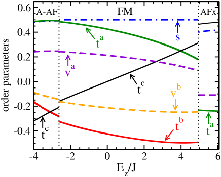
Figure 11: (Color online) Order parameters $\{s,t^{a,b,c},v^{a,b}\}$ for $\eta=0.28$ and $-4.0<E_{z}/J<6.0$ in the $A$-AF, FM and $G$-AF phases, from left to right.

Finally, we show the behavior of the order parameters $\{s,t^{a,b,c},v^{a,b}\}$ and the quantum fluctuation effects on them in the $A$-AF, FM and $G$-AF phases for $\eta=0.28$, see Fig. 11. The third orbital field $t^{c}$ is linearly dependent on $t^{a}$ and $t^{b}$ (by the constraint $t^{c}=-t^{a}-t^{b}$), and was added here to visualize the orbital order along the $c$ direction which is essential in the large $|E_{z}|$ regime showed in Fig. 11. In FM phase the spin order is saturated because of the lack of quantum and thermal fluctuation. For the same reason spin-orbital field factorizes and $\{v^{a},v^{b}\}$ fields bring no extra information which would not be already contained in $\{t^{a},t^{b}\}$. The overall behavior of $t^{c}$ is in agreement with the crystal field part of the Hamiltonian Eq. (7) with $t^{c}\to\pm 1/2$, giving uniform cigar or clover orbitals depending on the sign of $E_{z}$.

We emphasize that for increasing $E_{z}$ one finds two crossing points of $t^{c}$ with $\{t^{a},t^{b}\}$ curves, one at $t^{c}=t^{b}=-1/4$ and the other one at $t^{c}=t^{a}=1/4$. At these two points the orbitals take shapes of perfect clovers ($E_{z}<0$) or perfect cigars ($E_{z}>0$), with symmetry axes alternating in the $ab$ plane from site to site. Only one of these points belongs to the FM phase meaning that the four ”perfect” orbital configurations: AO order with clovers/cigars and FO order with clovers/cigars are separated by phase transitions in the spin-orbital model Eq. (7). The transitions shown in Fig. 11 are discontinuous due to the change of global spin order in each phase. The spin order parameter $s$ plays a role of staggered $A$-AF or AF magnetization in the extremal phases and is trivial (saturated) in the FM phase. On the other hand, all three phases displayed in Fig. 11 can be described by the same orbital sublattices assuming AO order. The large scale of $E_{z}$ in Fig. 11 is in contrast to those in other figures — it indicates that orbital degrees of freedom are very rigid when spins are almost frozen and one needs rather high energies to change their configuration.

V Nearest–neighbor correlations

V.1 Spin, orbital and spin-orbital correlations

Studying order parameters in different phases we get complete information about symmetry broken or disordered phases of the system, but this alone does not justify the use of the cluster MF method as order parameters can in principle be obtained using standard single-site MF approximation, see Sec. II.2. The advantage of the cluster method becomes evident when we investigate correlation functions on the bonds belonging to the considered cube. The most obvious ones are the spin–spin correlations $\langle{\bf S}_{i}\cdot{\bf S}_{j}\rangle$ or orbital–orbital correlations $\langle\tau^{\gamma}_{i}\tau^{\gamma}_{j}\rangle$, but in addition one may also determine joint spin-orbital correlations, $\langle({\bf S}_{i}\cdot{\bf S}_{j})\tau^{\gamma}_{i}\tau^{\gamma}_{j}\rangle$. Although one could in principle invent several other bond correlation functions, the above ones have the most transparent physical meaning because they enter the Hamiltonian. For the same reason we will only consider orbital correlation functions for different bond direction $\gamma=a,b,c$. This gives nine correlation functions, three in each direction, for each vertex of the cube. For symmetry reasons it is enough to consider only one chosen vertex, e.g. vertex number 1 in Fig. 4. For convenience we will use the following notation:

$$C_{s}^{\gamma} \equiv \langle{\bf S}_{1}\cdot{\bf S}_{i}\rangle,$$ (47)

$$C_{t}^{\gamma} \equiv \langle\tau^{\gamma}_{1}\tau^{\gamma}_{i}\rangle,$$ (48)

$$C_{st}^{\gamma} \equiv \langle({\bf S}_{1}\cdot{\bf S}_{i})\tau^{\gamma}_{1}\tau^{\gamma}_{i}\rangle,$$ (49)

where the bond $\langle 1i\rangle||\gamma$ and $i\in\{2,3,7\}$ which gives all nonequivalent nearest neighbor correlations along $\gamma=a,b,c$ (see Fig. 4).

In the next paragraphs we will present the numerical results for bond correlations $\{C_{s}^{\gamma},C_{t}^{\gamma},C_{st}^{\gamma}\}$ along different cuts of the phase diagram of Fig. 6. For all three–panel plots each panel describes correlation of one type: upper panel — spin correlations, middle one — orbital correlations, and bottom one — spin-orbital correlations. For each panel different characters (colors) of line indicate different direction $\gamma$: solid (red) line stands for $\gamma=c$, dashed (green) line for $\gamma=a$ and dashed–dotted (blue) line for $\gamma=b$. In case of two–panel plots there are only two directions considered, $c$ and $a$ because for symmetry reasons correlations along the $b$ and $a$ axes are identical. Therefore, the left panel concerns all three types of correlators for $\gamma=c$ and the right one for $\gamma=a$ in the way that solid (red) lines are spin–spin correlation functions, dashed (green) ones are orbital–orbital correlations and dashed–dotted (blue) represent spin-orbital correlators. In order to investigate the nature of spin-orbital entanglement we focus the discussion on two quantum phases which occur at finite values of Hund’s exchange $\eta$ near the orbital degeneracy: (i) the PVB phase, and (ii) the ESO phase.

V.2 Plaquette valence-bond phase

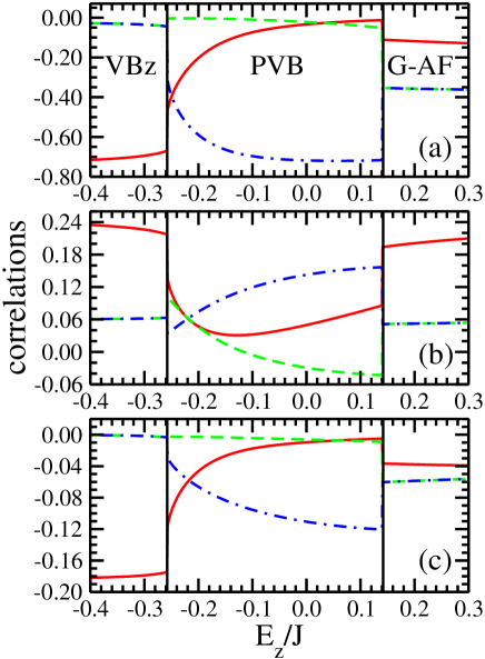
Figure 12: (Color online) Nearest neighbor correlations for $\eta=0.05$ and $-0.4<E_{z}/J<0.3$ in the VB$z$, PVB and $G$-AF phases. (a) Spin correlations: solid (red) line — $C_{s}^{c}$, dashed (green) line — $C_{s}^{a}$ and dashed–dotted (blue) line — $C_{s}^{b}$. (b) Orbital correlations: solid (red) line — $C_{t}^{c}$, dashed (green) line — $C_{t}^{a}$ and dashed–dotted (blue) line — $C_{t}^{b}$. (c) Spin-orbital correlations: solid (red) line — $C_{st}^{c}$, dashed (green) line — $C_{st}^{a}$ and dashed–dotted (blue) line — $C_{st}^{b}$.

We begin with bond correlation functions for $\eta=0.05$ and $-0.4<E_{z}/J<0.3$ in the VB$z$, PVB and $G$-AF phase. The $C_{s}^{c}$ function stays close to $-3/4$ in the VB$z$ phase while the other spin correlations are almost zero as one can expect in the interlayer singlet phase, see Fig. 12(a). After the first transition at $E_{z}\simeq-0.26J$ the situation changes — now the singlets are in $b$ direction and $C_{s}^{b}$ gets close to $-3/4$ when $E_{z}$ increases. After the second transition at $E_{z}\simeq 0.14J$ all the spin correlations take finite negative values with $C_{s}^{c}$ relatively weakest, keeping the symmetry between $a$ and $b$ direction. This is in agreement with the spin order in the $G$-AF phase discussed in Sec. IV.

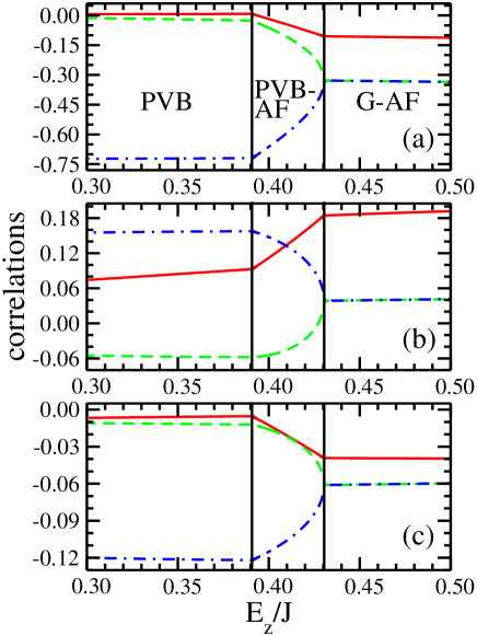
Figure 13: (Color online) Nearest neighbor correlations for $\eta=0.15$ and $0.3<E_{z}/J<0.5$ in the PVB, PVB-AF and $G$-AF phases. (a) Spin correlations: solid (red) line — $C_{s}^{c}$, dashed (green) line — $C_{s}^{a}$ and dashed–dotted (blue) line — $C_{s}^{b}$. (b) Orbital correlations: solid (red) line — $C_{t}^{c}$, dashed (green) line — $C_{t}^{a}$ and dashed–dotted (blue) line — $C_{t}^{b}$. (c) Spin-orbital correlations: solid (red) line — $C_{st}^{c}$, dashed (green) line — $C_{st}^{a}$ and dashed–dotted (blue) line — $C_{st}^{b}$.

The orbital correlation functions in the VB$z$ and $G$-AF phases behave as if the orbitals were frozen in uniform configuration with $t^{c}=\pm 1/2$ and $t^{a,b}=\mp 1/4$ whereas in the PVB phase their behavior is more nontrivial; the dominant $C_{t}^{b}$ is quite distant from its maximal value $1/4$ and the difference between $C_{t}^{a}$ and $C_{t}^{c}$ is visible, especially close to the $G$-AF phase, see Fig. 12(b). This result is due to quantum fluctuations: perfect VB$z$ and $G$-AF configurations are the exact eigenstates of the Hamiltonian, at least in the limit of large $|E_{z}|$, while perfect PVB state cannot be obtained exactly in any limit and gets easily destabilized by varying $E_{z}$. It is peculiar that the spin configuration is almost nonsensitive to the orbital splitting $E_{z}$ and the singlets stay rigid in the regime of spin disordered phases, i.e., below the transition to the $G$-AF phase. The spin-orbital sector, shown in Fig. 12(c), does not bring any new information; all the lines behave as if spin and orbital degrees of freedom were factorizable.

Figure 13 presents the bond correlations for a gradual transition between the PVB and $G$-AF phases, with an intermediate PVB-AF phase for $\eta=0.15$ and $0.3<E_{z}/J<0.5$. By decreasing $E_{z}$, i.e., looking from right to left, we can see the in–plane spin correlation bifurcating smoothly at the transition to the PVB-AF phase and evolving monotonically to the values characteristic of the PVB phase, see Fig. 13(a). The interplane spin correlations $C_{s}^{c}$ stay relatively weak everywhere which is obvious in both PVB and $G$-AF phase and hence not so surprising in the intermediate PVB-AF phase.

In the orbital sector we can see here very similar behavior to the one observed in Fig. 12 — again the order is far from the perfect PVB but $C_{t}^{c}$ is close to the classical value of $1/16$ obtained for the plane perpendicular to two directional orbitals along the $b$ axis, while $C_{t}^{a}$ is almost exactly opposite and $C_{t}^{b}$ stays below $1/4$, see Fig. 13(b). This shows some kind of universality at the transition from the PVB to $G$-AF phase which is independent of the intermediate phase. Again, the spin-orbital sectors, shown in Fig. 13(c), does not indicate any qualitatively new behavior comparing to spins and orbitals alone but looking at the phase diagrams with (Fig. 5) and without (Fig. 6) spin-orbital factorization we recognize that on-site spin-orbital entanglement must be responsible for the onset of the PVB-AF phase.

V.3 Phases with entangled spin-orbital order

Consider now smaller (negative) values of $E_{z}$, where unexpected and qualitatively new entangled phases occur in the phase diagram of Fig. 6. We display bond correlation functions in Fig. 14 in two neighboring highly frustrated and entangled phases, the ESO and EPVB phase — the latter one turns into the PVB phase when $E_{z}$ is increased. The relevant parameter range for $\eta=0.15$ is $-0.45<E_{z}/J<-0.1$. On the first glance this plot shows that the transitions between the ESO and EPVB as well as between the EPVB and PVB phases are of the second order. In the spin sector one observes weakening singlet order in the ESO phase with $C_{s}^{c}$ getting far from $-3/4$ and in-plane correlations $C_{s}^{a,b}$ being practically vanishing, see Fig. 14(a). After the first transition (at $E_{z}\simeq-0.36J$) $C_{s}^{b}$ grows rapidly toward negative values while $C_{s}^{c}$ goes to zero much more gently and $C_{s}^{a}$ stays close to zero. This means that in the EPVB phase we have relatively strong AF order in the $bc$ plane inside the cluster, turning into the $ac$ plane order on neighboring cubes. This gives finite magnetization $s$ shown in Fig. 9. When approaching the second transition (at $E_{z}\simeq-0.22J$) $C_{s}^{c}$ weakens and $C_{s}^{b}$ gets closer to $-3/4$ and this is continued within the PVB phase.

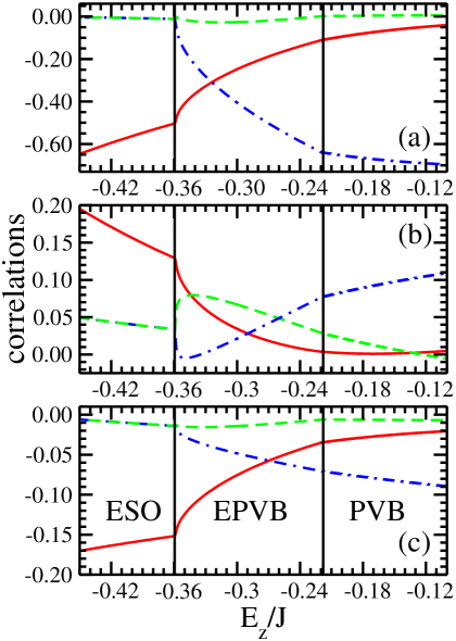
Figure 14: (Color online) Nearest neighbor correlations for $\eta=0.15$ and $-0.45<E_{z}/J<-0.1$ in the ESO, EPVB and PVB phases. (a) Spin correlations: solid (red) line — $C_{s}^{c}$, dashed (green) line — $C_{s}^{a}$ and dashed–dotted (blue) line — $C_{s}^{b}$. (b) Orbital correlations: solid (red) line — $C_{t}^{c}$, dashed (green) line — $C_{t}^{a}$ and dashed–dotted (blue) line — $C_{t}^{b}$. (c) Spin-orbital correlations: solid (red) line — $C_{st}^{c}$, dashed (green) line — $C_{st}^{a}$ and dashed–dotted (blue) line — $C_{st}^{b}$.

In the orbital sector we can find other differences between entangled and disentangled phases, see Fig. 14(b). In the ESO phase the $C_{t}^{c}$ drops considerably when approaching the first transition; this is in contrast with the VB$z$ phase where $C_{t}^{c}$ stays almost constant until the transition occurs. However, one finds that the spin-orbital bond correlation $C_{st}^{c}$ stays constant in the ESO phase, see Fig. 14(c). The behavior of in-plane correlation functions $C_{t}^{a,b}$ becomes somewhat puzzling within the EPVB phase: after bifurcation at the transition point $C_{t}^{b}$ drops to zero and slowly recovers to become dominant in the PVB phase, while $C_{t}^{a}$ stays dominant in certain region of the EPVB phase even though the spin correlations in $a$ direction vanish. Only $C_{t}^{c}$ gradually drops to zero throughout all three phases.

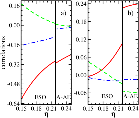
Figure 15: (Color online) Nearest neighbor correlations for $E_{z}=-0.43J$ and $0.15<\eta<0.25$ in the ESO and $A$-AF phases. (a) Correlations along the $c$ axis: solid (red) line — $C_{s}^{c}$, dashed (green) line — $C_{t}^{c}$ and dashed–dotted (blue) line — $C_{st}^{c}$. (b) Correlations within $ab$ planes: solid (red) line — $C_{s}^{a}$ , dashed (green) line — $C_{t}^{a}$ and dashed–dotted (blue) line — $C_{st}^{a}$. Correlations in $a$ and $b$ direction are the same.

Note that in the spin-orbital sector we can see the joint order in both entangled phases in a more transparent way than in the orbital one, at least concerning the ESO and EPVB phases (we should keep in mind that $-3/16\leq C_{st}^{\gamma}\leq 1/16$ while $-1/4\leq C_{t}^{\gamma}\leq 1/4$ where the bottom limit for $C_{st}^{\gamma}$ is realized only in singlet phases). The $C_{st}^{c}$ correlation is definitely dominant in the ESO phase and stays dominant in most of the EPVB phase in contrary to spin $C_{s}^{c}$ correlation. In addition, close to the second transition the $C_{st}^{c}$ correlation is overcome by $C_{st}^{b}$ which grows here stronger because of singlets being formed on the bonds along the $b$ axis. This tendency is further amplified within the PVB phase. Note that $C_{st}^{a}$ stays practically zero in all the phases shown in Fig. 14.

Now we turn to the dependence of bond correlations on increasing Hund’s exchange $\eta$. In Fig. 15 we display correlations for $E_{z}=-0.43J$ and $0.15<\eta<0.25$ in the ESO and $A$-AF phases. Both phases can be described by a strong tendency toward AO order with two sublattices which does not violate the $a$–$b$ symmetry inside the cube; for this reason we show only correlations along the $c$ and $a$ direction. The spin sector within the ESO phase is dominated by the decay of interplanar singlets accompanied by growth of in-plane correlations which triggers global $A$-AF order above the transition (at $\eta\simeq 0.22$). The orbital correlations in the $c$ direction drop almost to zero when $\eta$ grows and stay small in the $A$-AF phase. The in-plane orbital correlations $C_{t}^{a,b}$ decrease in the ESO phase too but remain finite after the transition. Summarizing, in the ESO phase close to the onset of the $A$-AF one we find a very weak orbital order accompanied by precursors of the $A$-AF order in spin sector.

Consider now the spin-orbital correlations. In the ESO phase $C_{st}^{c}$ takes relatively big, negative values and does not change much except for the transition point where it jumps to zero. In contrast, in the $A$-AF phase we no longer observe any spin-orbital ordering. Note that a peculiar signature of the ESO phase is rather robust spin-orbital order on the interlayer bonds along the $c$ axis which turns out to be more rigid against quantum fluctuations than orbital order and remains finite even when orbital order vanishes.

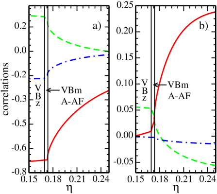
Figure 16: (Color online) Nearest neighbor correlations for $E_{z}=-0.72J$ and $0.10<\eta<0.25$ in the VB$z$, VBm and $A$-AF phases. (a) Correlations along the $c$ axis: solid (red) line — $C_{s}^{c}$, dashed (green) line — $C_{t}^{c}$ and dashed–dotted (blue) line — $C_{st}^{c}$. (b) Correlations within $ab$ plane: solid (red) line — $C_{s}^{a}$ , dashed (green) line — $C_{t}^{a}$ and dashed–dotted (blue) line — $C_{st}^{a}$. Correlations in $a$ and $b$ direction are the same.

In the last figure, Fig. 16, we display bond correlation functions in the VB$z$, VBm and $A$-AF phases for $E_{z}=-0.72J$ and $0.10<\eta<0.25$. As before, all the in-plane correlations are independent of $\gamma$. The plots prove that the transition from the VB$z$ to VBm phase is of the second order while the transition from the VBm to $A$-AF phase produces no discontinuities in correlations either, but the behavior of order parameters (see Fig. 10) is here slightly discontinuous. In the spin sector we observe first (at $\eta<0.17$) that robust singlets along the $c$ axis with $C_{s}^{c}\simeq-0.7$, see Fig. 16(a), are gradually weakened under increasing $\eta$ and weak FM correlations occur in the VB$z$ phase close to the first phase transition to the VBm order. We suggest that this regime of parameters could correspond to K₃Cu₂F₇, where the magnetic properties indicate interplanar singlets as formed in the VB$z$ and VBm phases accompanied by weak FM correlations in the $ab$ planes.Man07

Note that the changes in spin correlations with increasing $\eta$ become fast only after leaving the VBm phase. In the orbital sector perfect VB$z$ order dies out quickly already in the VBm regime, both on the bonds along the $c$ and $a$ axes. After entering the $A$-AF phase, $C_{t}^{c}$ vanishes exponentially while $C_{t}^{a}$ crosses zero and gradually falls to negative values. This behavior is in agreement with that shown in Fig. 10 saying that $t^{c}$ remains close to zero in the $A$-AF phase and the negative $C_{t}^{a}$ confirms AO order in $ab$ planes. Altogether, the spin-orbital sector does not exhibit here any considerable non-factorizable features.

VI Spin–orbital entanglement

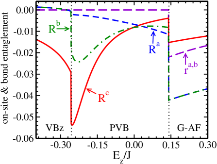
Figure 17: (Color online) On-site $r^{\gamma}$ Eq. (50) and bond $R^{\gamma}$ Eq. (51) entanglement parameters for $\eta=0.05$ and $-0.4<E_{z}<0.3$ in the VB$z$, PVB and $G$-AF phases.

The essence of spin-orbital entanglement observed in the cluster MF approach is spin-orbital non-factorizability. This feature can have either on-site or bond character, the latter was introduced in Ref. Ole06, . We emphasize that on-site entanglement which is characteristic for cases with finite spin-orbit coupling,Jac09 occurs also in the present superexchange model as shown below. We define the on-site entanglement as non-separability of the order parameters, i.e., spin and orbital operators are entangled when $v^{\gamma}\not=st^{\gamma}$, while the entanglement as being of bond type whenOle06 $C_{st}^{\gamma}\not=C_{s}^{\gamma}C_{t}^{\gamma}$, implying that it can be detected by investigating the respective correlation functions. Therefore we analyze in this Section the numerical results for the quantities (covariances) motivated by the above discussion which are defined as follows:

$$r^{\gamma} = v^{\gamma}-st^{\gamma}\,,$$ (50)

$$R^{\gamma} = C_{st}^{\gamma}-C_{s}^{\gamma}C_{t}^{\gamma}\,.$$ (51)

In case of $r^{\gamma}$ we consider only $\gamma=a,b$ as the on-site covariance satisfy the local constraint,

$$r^{c}=-r^{a}-r^{b},$$ (52)

while for $R^{\gamma}$ we shall present the data for $\gamma=a,b,c$. In order to quantify the above non-factorizability and to recognize whether it is strong or weak in a given phase, it is necessary to establish first the minimal and maximal values of $R^{\gamma}$ and $r^{\gamma}$. Simple algebraic considerations give the following inequalities: the bond covariances $|R^{\gamma}|<0.25$ in singlet phases, $|R^{\gamma}|<0.125$ in phases with magnetic order, and the on-site covariances $|r^{\gamma}|<0.25$ everywhere.

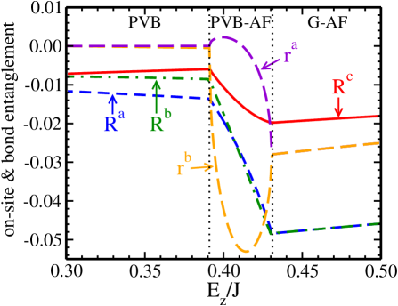
Figure 18: (Color online) On-site $r^{\gamma}$ Eq. (50) and bond $R^{\gamma}$ Eq. (51) entanglement parameters for $\eta=0.15$ and $0.3<E_{z}/J<0.5$ in the PVB, PVB-AF and $G$-AF phases.

First of all, the numerical results show that both bond Eq. (51) and on-site Eq. (50) spin-orbital entanglement is small in the regime of weak Hund’s exchange coupling. This feature is illustrated in Fig. 17 for the VB$z$, PVB and $G$-AF phases at $\eta=0.05$ and $-0.4<E_{z}/J<0.3$. The $r^{a}=r^{b}$ curves show no on-site spin-orbital entanglement ($r^{\gamma}=0$) in both VB$z$ and PVB phases, while it is finite in the $G$-AF phase ($r^{a}=r^{b}<0$) and gradually approaches zero with increasing $E_{z}$. We emphasize that this on-site non-factorizability is minute, being one order of magnitude smaller than its maximal value, and does not play any important role for the stability of the $G$-AF ground state. This is confirmed by the fact that $G$-AF phase exists in the same region of parameters in both phase diagrams: factorizable (Fig. 5) and non-factorizable one (Fig. 6), and occurs even in the single-site MF approximation (Fig. 3). It is interesting to note that the in-plane bond entanglement $R^{a,b}$ takes relatively high values in the $G$-AF phase. This is clearly an effect of quantum fluctuations; the perfect (classical) $G$-AF phase of Fig. 3 has uniform fixed $x$ orbital configuration with $t^{c}=1/2$ which suppresses any non-factorizability. As the on-site entanglement, also the bond spin-orbital entanglement vanishes gradually for high values of $E_{z}\to\infty$.

At the border line between the VB$z$ and PVB phases we noticed a considerable increase of $R^{c}$ and less pronounced growth of $R^{b}$ which seem to be induced by the transition as the $R^{b,c}$ drop quickly for higher values of $E_{z}$. In the VB$z$ phase we expect all the spin-orbital covariances to be zero for the same reasons as in the $G$-AF phase and this also applies to the perfect PVB phase. In Fig. 17, however, the VB$z$ and PVB phases are dominated by the critical behavior which distorts perfect orderings.

Also in the regime of higher Hund’s exchange interaction $\eta=0.15$ the spin-orbital covariances in the PVB, PVB-AF and $G$-AF phases are small in the range of their stability, see Fig. 18 for $0.3<E_{z}/J<0.5$. In the PVB phase all the covariances take small values showing that the PVB type of order has no serious quantum fluctuations in this parameter range. The on-site covariances $\{r^{a},r^{b}\}$ bifurcate from the zero value at the first transition and this emergence of non-factorizability stabilizes here the intermediate PVB-AF phase (compare Figs. 5 and 6) and persists in the $G$-AF phase where they overlap again ($r^{a}=r^{b}$). In the regime of PVB-AF phase we observe also almost linear decrease of the in-plane $R^{a,b}$ staying close to each other and a smaller drop of $R^{c}$. Although these quantities are all small, the order parameters (see Fig. 8) are small too, so we conclude that spin-orbital entanglement is qualitatively important here. The minimum of all $R^{\gamma}$ is located at the second transition indicating that highly entangled states play a role also at the onset of the $G$-AF phase.

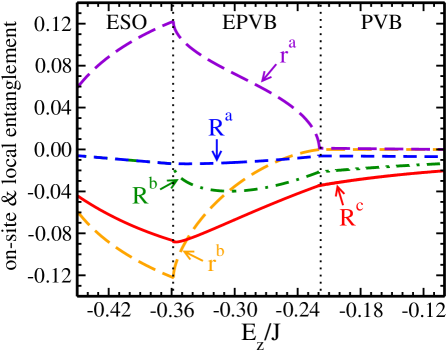
Figure 19: (Color online) On-site $r^{\gamma}$ Eq. (50) and bond $R^{\gamma}$ Eq. (51) entanglement parameters for $\eta=0.15$ and $-0.45<E_{z}/J<-0.1$ in the ESO, EPVB and PVB phases.

Figure 19 shows spin-orbital entanglement in the most exotic part of the phase diagram with the ESO, EPVB and PVB phases for $\eta=0.15$ and $-0.45<E_{z}/J<-0.1$. The on-site spin-orbital covariances $\{r^{a},r^{b}\}$ take high, opposite values in both the ESO and EPVB phase, with maximum (minimum) at the transition line between them. Comparing to other phases $r^{a,b}$ values are highest in the ESO and EPVB phases, and comparing the two phase diagrams in Figs. 5 and 6, we recognize that spin-orbital entanglement is a constitutive feature of both ESO and EPVB states. We emphasize that the on-site spin-orbital entanglement is strong and complementary in the ESO phase on the bonds along the $a$ and $b$ direction ($r^{a}=-r^{b}$), while it vanishes between the $ab$ planes ($r^{c}=0$). These results indicate spin-orbital fluctuations in the $ab$ planes, with $\langle S^{z}\sigma^{x}\rangle\neq 0$ and no fluctuations along the $c$ axis, where $r^{c}$ follows from $\langle S^{z}\sigma^{z}\rangle=0$. In contrast, in the EPVB phase there is also finite on-site entanglement for the interlayer order parameters, $r^{c}\neq 0$.

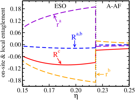
Figure 20: (Color online) On-site $r^{\gamma}$ Eq. (50) and bond $R^{\gamma}$ Eq. (51) entanglement parameters for $E_{z}=-0.43J$ and $0.15<\eta<0.25$ in the ESO and $A$-AF phases.

Looking at the bond parameters $R^{\gamma}$ we see that the dominant one is $R^{c}$ falling gradually in the ESO down to the minimum at the ESO-EPVB transition. At the same point $R^{b}$ drops from zero value in the ESO phase and takes maximally negative value inside the EPVB regime. In contrast, $R^{a}$ remains close to zero in the entire regime of parameters and in the PVB all the covariances go to zero showing that the order within the PVB phase is practically disentangled. The dominant role of $R^{c}$ comes from the $c$–axial symmetry of the ESO phase and increased quantum fluctuations on the ESO-EPVB border while the non-zero value of $R^{b}$ in the EPVB phase follows from the magnetic and orbital order on the cube in the $bc$ plane mentioned in the previous section.

When Hund’s exchange is increased across the transition between the ESO and $A$-AF phases, one finds that bond and on-site spin-orbital covariances are radically different in both phases, see Fig. 20. The plot shows that the ESO phases is much stronger entangled than the $A$-AF one where all the covariances stay close to zero. Only the in-plane $R^{a,b}$ parameters are small also in the ESO phase but the other covariances, including the bond covariance along the $c$ axis $R^{c}$, take considerable values.

Finally, we focus on the range of large negative crystal field splitting $E_{z}=-0.72J$ and display the spin-orbital covariances in the VB$z$, VBm and $A$-AF phases for increasing Hund’s exchange $0.15<\eta<0.25$, see Fig. 21. On the one hand, looking at the VBm region of the plot we can understand why this phase can exist when factorized spin-orbital MF is applied (again, compare Figs. 5 and 6); the on-site covariances $\{r^{a},r^{b}\}$ vanish here and within the VB$z$ phase. On the other hand, one finds certain on-site entanglement in the $A$-AF phase, especially close to the transition line — this shows why the $A$-AF area is expanded in Fig. 6 as compared with the non-factorized phase diagram of Fig. 5. Concerning bond entanglement, it is significant (finite $R^{c}<0$) only along the interlayer $c$ bonds in all these three phases, taking maximal values of $|R^{c}|$ in the $A$-AF phase. One can understand this as follows: in the VB$z$ phase the orbital order is almost perfect and orbitals stay frozen — therefore spin-orbital factorization is here almost exact as indicated by a low value of $R^{c}$. This is not the case in the $A$-AF phase where orbitals fluctuate, especially close to the transition line to the VBm phase. The $R^{a,b}$ bond parameters are small due to the imposed FM order within the $ab$ planes which decouples the spin from orbital fluctuations on the bonds along the $a$ and $b$ directions.

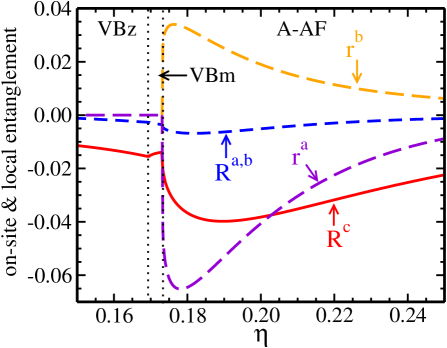
Figure 21: (Color online) On-site $r^{\gamma}$ Eq. (50) and bond $R^{\gamma}$ Eq. (51) entanglement parameters for $E_{z}=-0.72J$ and $0.15<\eta<0.25$ in the VB$z$, VBm and $A$-AF phases.

VII Discussion and summary

The numerical results presented in the last three sections, obtained using the sophisticated mean-field approach with an embedded cubic cluster, provide a transparent and rather complete picture of possible ordered and disordered phases in the bilayer spin–orbital $d^{9}$ model. This approach is well designed to determine the character of spin, orbital and spin-orbital order and correlations in all the discussed phases as it includes the most important quantum fluctuations on the bonds and captures the essential features of spin-orbital entanglement. By analyzing order parameters we also presented evidence which allowed us to identify essential features of different phases and to distinguish between first and second order phase transitions. This is especially important in cases when two phases are separated by an intermediate configuration, such as the PVB-AF or VBm phase, where one finds a gradual evolution from singlet to AF correlations, supported (or not) by non-factorizable spin-orbital order parameter. We believe that the cluster mean-field approach presented here and including thie joint spin-orbital order parameter is more realistic because there is no physical reason, apart from the form of the $d^{9}$ Hamiltonian, to treat spin and orbital operators as the only fundamental symmetry-breaking degrees of freedom in any phase.

Interestingly, the results show that the bottom part of the phase diagram of the $d^{9}$ spin-orbital model does not exhibit any frustration or spin-orbital entanglement up to $\eta\simeq 0.07$ and the type of spin and orbital order are chosen there predominantly by the crystal field term $\propto E_{z}$. Quantum fluctuations dominate at $E_{z}\simeq 0$ and for $E_{z}<0$, where they stabilize either in-plane or interplanar spin singlets accompanied by directional orbitals which stabilize them. These two phases are reminiscent of the resonating valence-bond (RVB) phase and PVB phase found in the 3D spin-orbital $d^{9}$ model.Fei97 Here, however, the VB$z$ phase extends down to large values of $E_{z}$, where instead the long-range order in the $G$-AF$z$ phase was found in the 3D model. This demonstrates that interlayer quantum fluctuations are particularly strong in the present bilayer case. On the contrary, at $E_{z}>0$ one finds the $G$-AF spin order which coexists with FO order of $x$ orbitals. It is clear that both the VB$z$ and $G$-AF phase are favored by the interplay of lattice geometry and by the shape of occupied orbitals for $E_{z}\to\pm\infty$. In this low-$\eta$ regime of the diagram the area occupied by the PVB phase is narrow and especially orbital order is affected by the quantum critical fluctuations. The planar singlets are formed shortly after leaving the VB$z$ phase and remain stable afterwards. Spin-orbital non-factorizability seems to be marginal in the entire VB$z$ phase but plays certain role when switching to the planar singlet phase, especially visible for the interplane bond covariance $R^{c}$.

On the contrary, in the PVB phase away from the critical regime spin-orbital non-factorizability vanishes and suddenly reappears in the $G$-AF phase, not as a transition effect but rather as a robust feature vanishing only for high values of $E_{z}$. We argue that this is related with surprisingly rigid interplane spin-spin correlations which should, if we think in spin-orbital factorizable way, decay quickly as $t^{c}$ approaches $1/2$. Following this ”factorizable reasoning” we could also expect stability of the $C$-AF phase for higher values of $\eta$, above the $G$-AF phase. These effects are absent in our results, showing that intuition suggesting spin-orbital factorization can be misleading even when considering such a simple isotropic orbital configuration.

For higher values of Hund’s exchange $\eta$ frustration increases when AF exchange interactions compete with FM ones, and as a result the most exotic phases with explicit on-site spin-orbital entanglement arise; two of them, the ESO and EPVB phase are neighboring and placed in between the VB$z$ and PVB ones, and they become degenerate with both of them at the multicritical point where four phases meet (see Fig. 6). This situation follows from the fact that singlet phases are more susceptible to ferromagnetism favored by high $\eta$ than the $G$-AF phase is, which turned out to be surprisingly robust. The ESO phase is also a singlet phase similar to the VB$z$ one but with spin singlets and orbital order gradually suppressed under increasing Hund’s exchange $\eta$. At the same time spin-orbital order stays almost constant and spin-orbital entanglement grows.

Further increase of $\eta$ always leads to the $A$-AF phase throughout a discontinuous transition accompanied by an abrupt drop of spin-orbital entanglement. Above $\eta\simeq 0.2$ the ESO phase is completely immersed in the $A$-AF one and ends up with a single bicritical point. If we come back below $\eta\approx 0.2$ then the ESO changes smoothly into the EPVB phase, being an entangled precursor of the PVB order, meaning that the non-uniform orbital order and in-plane singlets are formed and spin-orbital entanglement drops. On the other hand, this phase can be also seen as an extension of the $A$-AF into fully AF sector because the EPVB phase has long-range magnetic order, being however strongly non-uniform (see Fig. 14).

Finally, we would like to remark that experimental phase diagrams of strongly correlated transition metal oxides are one of the challenging directions of recent research. Systematic trends observed for the onset of the magnetic and orbital order in the $R$VO₃ perovskites have been successfully explained by the competing interactions in presence of spin-orbital entanglement.Hor08 In contrast, the theory could not explain exceptionally detailed information on the phase diagram of the $R$MnO₃ manganites which accumulated due to impressive experimental work.Goo06 The present K₃Cu₂F₇ bilayer system is somewhat similar to La_2-2xSr_1+2xMn₂O₇ bilayer manganites with very rich phase diagrams and competition between phases with different types of long-range order in doped systems.bilay Such phases are generic in transition metal oxides and were also reproduced in models of bilayer manganites which have to include in addition superexchange interaction between core $t_{2g}$ spinsOle03 ; Dag06 that suppresses spin-orbital fluctuations and entanglement in the $e_{g}$ subsystem. In contrast, K₃Cu₂F₇ bilayer is rather unique as the only electronic interactions arise here due to entangled spin-orbital superexchange. They explain the origin of the VB$z$ phase observedMan07 in K₃Cu₂F₇ but not found in bilayer manganites, and provide a unique opportunity of investigating whether signatures of spin-orbital entanglement could be identified in future experiments.

Summarizing, the presented analysis demonstrates that spin-orbital entanglement plays a crucial role in complete understanding of the phase diagram of the bilayer spin-orbital $d^{9}$ model. By introducing additional spin-orbital order parameter independent of spin and orbital mean fields we obtained phases with spin disorder in highly frustrated regime of parameters. The example of the entangled ESO and EPVB phases shows that joint spin-orbital order can be at least as strong as the other two (spin or orbital) types of order, or may even persist as the only symmetry breaking field when the remaining ones vanish. We argue that the cluster method we used here is sufficiently realistic to investigate the phase diagram of the 3D spin-orbital $d^{9}$ model, and could be applied to other spin-orbital superexchange models adequate for undoped transition metal oxides.

Appendix A Solution of the mean-field equations

Here we present briefly the solution of the self-consistency Eqs. (24) and (25) obtained in the single-site MF approximation. It is obtained as follows: assuming $a$–$b$ symmetry of the system, i.e., putting $\chi^{a}=\chi^{b}$ and $\xi^{a}=\xi^{b}$, we derive $t^{a}$ and $t^{c}$ from Eq. (23) as functions of $\alpha$ and $\beta$,

$$t^{c} = 4g\alpha+2gE_{z}+g_{1},$$ (53)

$$t^{a} = -2g\alpha-\frac{2\beta}{\sqrt{3}}g_{2}-\frac{1}{2}(2gE_{z}+g_{1}),$$ (54)

with

$$g = (\chi^{a}-\xi^{a}+2\chi^{c}-2\xi^{c})^{-1},$$ (55)

$$g_{1} = g(\xi^{a}-\xi^{c}),$$ (56)

$$g_{2} = (\chi^{a}-\xi^{a})^{-1}.$$ (57)

Now we introduce a parametrization

$$\alpha=\Delta\sin\phi,\hskip 28.45274pt\beta=\Delta\cos\phi,$$ (58)

and use the self-consistency Eqs. (24) and (25). From $t^{c}$ one finds immediately $\sin{\phi}$ depending on $\Delta$,

$$\sin{\phi}=-2\,\frac{2gE_{z}+g_{1}}{8g\Delta+1}.$$ (59)

Comparing Eqs. (24) and (53) for $t^{a}$ one gets:

$$\sin\phi-\sqrt{3}\cos{\phi}=$$ (60)

$$- 4\left(2g\Delta\sin{\phi}+\frac{2}{\sqrt{3}}g_{2}\Delta\cos{\phi}+gE_{z}+\frac{1}{2}g_{1}\right).$$

After inserting $\sin{\phi}$ into Eq. (60) we obtain a surprisingly simple result for $\cos{\phi}$:

$$\cos{\phi}\left(\Delta-\frac{3}{8g_{2}}\right)=0.$$ (61)

This leads to two classes of solutions of self-consistency Eqs. (24) and (25): (i) either $\cos{\phi}=0$, or (ii) $\Delta=3/8g_{2}$ and $\cos{\phi}\not=0$. The first option implies $\sin{\phi}=\pm 1$ and leads to two uniform orbital configurations with $t^{c}=\mp\frac{1}{2}$ and $t^{a}=t^{b}=-t^{c}/2$. Furthermore, using Eq. (59) we can calculate $\Delta$ and find the borders of these uniform phases demanding $\Delta\geq 0$.

The second option, i.e., $\cos{\phi}\not=0$, implies AO-type of order with:

$$t_{c}\!\! = \!\frac{2gE_{z}+g_{1}}{3g/g_{2}+1},$$ (62)

$$t_{a}\!\! = \!-\frac{1}{2}\frac{2gE_{z}+g_{1}}{3g/g_{2}+1}\mp\frac{\sqrt{3}}{2}\sqrt{\frac{1}{4}-\left(\frac{2gE_{z}+g_{1}}{3g/g_{2}+1}\right)^{2}},$$ (63)

and with phase borders defined by the condition: $2|t^{c}|\leq 1$. The phase borders given here set the maximal range of the phase under consideration and cannot be treated as the lines of phase transitions shown in the phase diagram; the latter lines are determined by comparing the ground state energies $E_{0}$ calculated form Eq. (26).

References

- (1) L. F. Feiner, A. M. Oleś, and J. Zaanen, Phys. Rev. Lett. 78, 2799 (1997).
- (2) K. I. Kugel and D. I. Khomskii, Usp. Fiz. Nauk 136, 621 (1982) [Sov. Phys. Usp. 25, 231 (1982)].
- (3) Y. Tokura and N. Nagaosa, Science 288, 462 (2000).
- (4) G. Khaliullin, Prog. Theor. Phys. Suppl. 160, 155 (2005); A. M. Oleś, Acta Phys. Polon. A 115, 36 (2009) [http://przyrbwn.icm.edu.pl/APP/PDF/115/a115z1006.pdf].
- (5) J. van den Brink, Z. Nussinov, and A. M. Oleś, in: Introduction to Frustrated Magnetism: Materials, Experiments, Theory, edited by C. Lacroix, P. Mendels, and F. Mila, Springer Series in Solid-State Sciences, Vol. 164 (Springer, New York, 2011), pp. 631-672.
- (6) J. Zaanen and A. M. Oleś, Phys. Rev. B48, 7197 (1993).
- (7) L. F. Feiner and A. M. Oleś, Phys. Rev. B59, 3295 (1999); P. Benedetti and R. Zeyher, ibid. 59, 9923 (1999).
- (8) A. M. Oleś, P. Horsch, G. Khaliullin, and L. F. Feiner, Phys. Rev. B72, 214431 (2005).
- (9) J. Deisenhofer, I. Leonov, M. V. Eremin, Ch. Kant, P. Ghigna, F. Mayr, V. V. Iglamov, V. I. Anisimov, and D. van der Marel, Phys. Rev. Lett. 101, 157406 (2008).
- (10) N. Binggeli and M. Altarelli, Phys. Rev. B70, 085117 (2004); I. Leonov, D. Korotin, N. Binggeli, V. I. Anisimov, and D. Vollhardt, ibid. 81, 075109 (2010).
- (11) D. I. Khomskii and M. V. Mostovoy, J. Phys. A 36, 9197 (2003); Z. Nussinov, M. Biskup, L. Chayes, and J. van den Brink, Europhys. Lett. 67, 990 (2004); B. Douçot, M. V. Feigel’man, L. B. Ioffe, and A. S. Ioselevich, Phys. Rev. B71, 024505 (2005); J. Dorier, F. Becca, and F. Mila, ibid. 72, 024448 (2005).
- (12) S. Wenzel and W. Janke, ibid. 78, 064402 (2008); S. Wenzel, W. Janke, and A. M. Läuchli, Phys. Rev. E81, 066702 (2010).
- (13) Z. Nussinov and G. Ortiz, Europhys. Lett. 84, 36005 (2008); F. Trousselet, A. M. Oleś, and P. Horsch, ibid. 91, 40005 (2010).
- (14) R. Orús, A. C. Doherty, and G. Vidal, Phys. Rev. Lett. 102, 077203 (2009); W. Brzezicki and A. M. Oleś, Phys. Rev. B82, 060401 (2010); L. Cincio, J. Dziarmaga, and A. M. Oleś, ibid. 82, 104416 (2010).
- (15) Wen-Long You, Guang-Shan Tian, and Hai-Qing Lin, J. Phys. A 43, 275001 (2010).
- (16) J. van der Brink, P. Horsch, F. Mack, and A. M. Oleś, Phys. Rev. B59, 6795 (1999); J. van der Brink, New J. Phys. 6, 201 (2004); J. van der Brink, P. Horsch, and A. M. Oleś, Phys. Rev. Lett. 85, 5174 (2000); A. van Rynbach, S. Todo, and S. Trebst, ibid. 105, 146402 (2010).
- (17) Wen-Long You, Guang-Shan Tian, and Hai-Qing Lin, Phys. Rev. B75, 195118 (2007).
- (18) B. Normand and A. M. Oleś, Phys. Rev. B78, 094427 (2008); B. Normand, ibid. 83, 064413 (2011); J. Chaloupka and A. M. Oleś, ibid. 83, 094406 (2011).
- (19) F. Vernay, K. Penc, P. Fazekas, and F. Mila, Phys. Rev. B70, 014428 (2004); F. Vernay, A. Ralko, F. Becca, and F. Mila, ibid. 74, 054402 (2006); F. Mila, F. Vernay, A. Ralko, F. Becca, P. Fazekas, and K. Penc, J. Phys. Condens. Matter 19, 145201 (2007); A. Reitsma, L. F. Feiner, and A. M. Oleś, New J. Phys. 7, 121 (2005).
- (20) J. B. Goodenough, Magnetism and the Chemical Bond (Interscience, New York, 1963); J. Kanamori, J. Phys. Chem. Solids 10, 87 (1959).
- (21) D. A. Tennant, T. G. Perring, R. A. Cowley, and S. E. Nagler, Phys. Rev. Lett. 70, 4003 (1993); S. E. Nagler, D. A. Tennant, R. A. Cowley, T. G. Perring, and S. K. Satija, Phys. Rev. B44, 12361 (1991); D. A. Tennant, R. A. Cowley, S. E. Nagler, and A. M. Tsvelik, ibid. 52, 13368 (1995).
- (22) B. Lake, D. A. Tennant, and S. E. Nagler, Phys. Rev. B71, 134412 (2005); B. Lake, D. A. Tennant, C. D. Frost, and S. E. Nagler, Nature Materials 4, 329(2005).
- (23) R. Caciuffo, L. Paolasini, A. Sollier, P. Ghigna, E. Pavarini, J. van den Brink, and M. Altarelli, Phys. Rev. B65, 174425 (2002).
- (24) A. M. Oleś, L. F. Feiner, and J. Zaanen, Phys. Rev. B61, 6257 (2000).
- (25) G. Khaliullin and V. Oudovenko, Phys. Rev. B56, R14243 (1997); L. F. Feiner, A. M. Oleś, and J. Zaanen, J. Phys.: Condens. Matter 10, L555 (1998).
- (26) T. N. De Silva, A. Joshi, M. Ma, and F. C. Zhang, Phys. Rev. B68, 184402 (2003).
- (27) A. M. Oleś, P. Horsch, L. F. Feiner, and G. Khaliullin, Phys. Rev. Lett. 96, 147205 (2006).
- (28) B. Frischmuth, F. Mila, and M. Troyer, Phys. Rev. Lett. 82, 835 (1999); Yan Chen, Z. D. Wang, Y. Q. Li, and F. C. Zhang, Phys. Rev. B75, 195113 (2007); A. M. Oleś, P. Horsch, and G. Khaliullin, Phys. Status Solidi B 244, 2378 (2007).
- (29) G. Khaliullin, P. Horsch, and A. M. Oleś, Phys. Rev. B70, 195103 (2004).
- (30) P. Horsch, A. M. Oleś, L. F. Feiner, and G. Khaliullin, Phys. Rev. Lett. 100, 167205 (2008).
- (31) C. Ulrich, G. Khaliullin, J. Sirker, M. Reehuis, M. Ohl, S. Miyasaka, Y. Tokura, and B. Keimer, Phys. Rev. Lett. 91, 257202 (2003); P. Horsch, G. Khaliullin, and A. M. Oleś, ibid. 91, 257203 (2003).
- (32) J. Sirker, A. Herzog, A. M. Oleś, and P. Horsch, Phys. Rev. Lett. 101, 157204 (2008).
- (33) A. M. Oleś, J. Zaanen, and P. Fulde, Physica B&C 148, 260 (1987); A. M. Oleś and W. Grzelka, Phys. Rev. B44, 9531 (1991).
- (34) A. K. McMahan, J. F. Annett, and R. M. Martin, Phys. Rev. B42, 6268 (1990); J. B. Grant and A. K. McMahan, ibid. 46, 8440 (1992).
- (35) G. Jackeli and N. B. Perkins, Phys. Rev. B65, 212402 (2002); A. M. Oleś and L. F. Feiner, ibid. 67, 092407 (2003); K. Rościszewski and A. M. Oleś, J. Phys. Condens. Matter 20, 365212 (2008).
- (36) M. Daghofer, A. M. Oleś, D. M. Neuber, and W. von der Linden, Phys. Rev. B73, 104451 (2006).
- (37) Von E. Herdtweck and D. Babel, Z. Anorg. Allg. Chem. 474, 113 (1981).
- (38) H. Manaka, Y. Miyashita, Y. Watanabe, and T. Masuda, J. Phys. Soc. Jpn. 76, 044710 (2007).
- (39) A. M. Oleś, Phys. Rev. B28, 327 (1983).
- (40) A. I. Lichtenstein, V. I. Anisimov, and J. Zaanen, Phys. Rev. B52, R5467 (1995); J. E. Medvedeva, M. A. Korotin, V. I. Anisimov, and A. J. Freeman, ibid. 65, 172413 (2002).
- (41) For convenience, we use here the same notation for the multiplet coefficients as in Ref. Ole05, .
- (42) G. Jackeli and G. Khaliullin, Phys. Rev. Lett. 102, 017205 (2009); 103, 067205 (2009).
- (43) J.-S. Zhou and J. B. Goodenough, Phys. Rev. Lett. 96, 247202 (2006).
- (44) M. Medarde, J. F. Mitchell, J. E. Millburn, S. Short, and J. D. Jorgensen, Phys. Rev. Lett. 83, 1223 (1999); M. Kubota, H. Fujioka, K. Hirota, K. Ohoyama, Y. Moritomo, H. Yoshizawa, and Y. Endoh, J. Phys. Soc. Jpn. 69, 1606 (2000); C. D. Ling, J. E. Millburn, J. F. Mitchell, D. N. Argyriou, J. Linton, and H. N. Bordallo, Phys. Rev. B62, 15096 (2000)