Dynamical Symmetry Breaking with Four-Superfield Interactions

Abstract

We investigate the dynamical mass generation resulted from interaction terms with four chiral superfields. The kind of interactions maybe considered a supersymmetric generalization of the four-fermion interactions of the classic Nambu–Jona-Lasinio model. A four-superfield interaction that contains a four-fermion interaction as one of its component terms has been the standard supersymmetrization of the NJL model for decades. Recently, we introduced a holomorphic variant with a dimension five interaction term instead. The latter is a main target of the present analysis. With the introduction of a new perspective on the superfield gap equation, we derive it for each one of the four-superfield interactions, using the supergraph technique. Through analyzing solutions to the gap equations, we illustrate the dynamical generation of superfield Dirac mass, including a supersymmetry breaking part. A dynamical symmetry breaking generally goes along with the dynamical mass generation, for which a bi-superfield condensate is responsible. The explicit illustration of dynamical symmetry breaking from the holomorphic dimension five interaction is reported for the first time. It has rich and novel features, which would be easily missed without the superfield approach developed here. We also discuss the nature of the bi-superfield condensate and its role of the effective Higgs superfield picture for both cases, illustrating their difference. Note that such a holomorphic quark superfield interaction term can successful account for the electroweak symmetry breaking with Higgs superfields as composites.

I Introduction

Dynamical mass generation and symmetry breaking is a very interesting theoretical topic with important phenomenological applications. In the early studies of mechanism for spontaneous symmetry breaking, Nambu adopted the idea of Cooper pairing Nobel to construct a classic model of dynamical mass generation and symmetry breaking. This is the Nambu–Jona-Lasinio (NJL) model Nambu:1961tp , with a strong attractive four-fermi interaction. It can be shown through the analysis of the nonperturbative gap equation that the interaction induces a bi-fermion vacuum condensate which serves as the source for the fermion Dirac mass. The condensate naturally breaks whatever symmetry the bi-fermion configuration carries a nontrivial quantum number of. The classic example is the (Dirac fermion) chiral symmetry, which was Nambu’s first concern Nobel ; N60 . After the Standard Model was generally established, the exact mechanism of electroweak symmetry breaking became a problem of paramount importance in the phenomenological domain. It is still open till today. It was pointed out by Nambu Nambu that for a sufficiently heavy top quark, an NJL model of top condensate can give rise to electroweak symmetry breaking. The top quark, however, turns out to be not heavy enough tSM ; Chung:2005yz .

Supersymmetry is another important theme in modern physics. The idea of constructing a supersymmetric version of the NJL model was introduced in 1982 BL . A dimension six four-superfield interaction containing the NJL four-fermion interaction was the basic feature. The superfield gap equation analysis however showed no nontrivial mass solution. The model supplemented with soft supersymmetric breaking mass terms was later established, through an effective potential analysis of its effective theory with auxiliary Higgs superfield introduced, to success in giving dynamical mass generation BE . A direct gap equation analysis from the original model Lagrangian, however, has not been available. On the side of phenomenological applications, a gauged version of the kind of model was presented for electroweak symmetry breaking, giving the supersymmetric Standard Model as the low-energy effective theory CLB ; 92 . Supersymmetry fixes the unnatural fine tuning of the four-fermion coupling required in the NJL model of top condensation. Phenomenological viability of the model has been severely unfavorable cornered with the relatively small top mass value determined and constraint on the $\tan\!\beta$ parameter 034 .

In a re-examination of the supersymmetrization of the NJL model, it was realized that there is a natural alternative to the one given in Refs.BL ; BE , as elaborated in Ref.035 . The alternative was presented in Ref.034 , together with an explicit model version that can give rise to electroweak symmetry breaking. The new model has a dimension five four-superfield interaction instead. The interaction is a superpotential term, hence holomorphic. It was named the holomorphic supersymmetric Nambu–Jona-Lasinio (HSNJL) model, while the the name supersymmetric Nambu–Jona-Lasinio (SNJL) model is kept for the dimension six version. The HSNJL model for electroweak symmetry breaking is a gauged version with two composite superfields. It also gives rise to the supersymmetric Standard Model as the low-energy effective theory. A first step renormalization group analysis was presented to illustrate the basic compatibility of the current experimental constraints on the latter model with the HSNJL model features. We are interested in establishing the dynamical mass generation for the generic HSNJL model structure, with a direct gap equation analysis. More generally, we seek to obtain gap equation results for both the dimension five and dimension six four-superfield interactions. We success in doing that, only with the development of a new perspective on the superfield gap equation. We obtain gap equations and dynamical mass generation results for both cases with generic couplings. For the case with the dimension five interaction, our analysis here mostly focused on the simplest version of a HSNJL model, with one superfield composite. Generalization to the two composite case should be straight forward. For the dimension six case, we obtain a supersymmetric breaking part of the dynamical mass generation not available before.

Our calculational framework is based on the supergraph techniques of Grisaru, Siegel and Roček GSR , with extension to fully accommodate supersymmetric breaking effect as developed by Miller M , Helayel-Neto H , Scholl S , and others. In a way, we take it a step further. All couplings, including mass terms, in the superfield Lagrangian are considered like constant superfields, i.e. with in general both a supersymmetric parts and a (soft) supersymmetry breaking parts. The effective action may then be considered as a superfield functional with explicit dependence on the Grassmannian coordinates $\theta$ and $\bar{\theta}$, hence also having supersymmetric and supersymmetry breaking parts. In particular, we will calculate the proper self-energy with its supersymmetric part and supersymmetry breaking part to obtain the gap equation for a model as a pair of coupled equations involving both the corresponding supersymmetric and supersymmetry breaking parts of the Dirac mass parameter. Note that the supersymmetric part contribute to the usual fermion Dirac mass as well as mass-squared for the two scalar field components, while the supersymmetry breaking part contributes to the mass mixing between the scalars. One will see that the approach is powerful for a comprehensive analysis of the general case of the parameter value. If one considers only the parameter $m$ it will leads to the wrong, or at least in complete, answer.

Our gap equation analysis will be presented in Sec.II, which is the main content of the paper. In Sec.III, we discussed some details of the mass generation and symmetry breaking features, after which we conclude in Sec.IV.

II Dynamical Mass Generation — Gap Equation Analysis

We start with the following Lagrangian density for what one wants to have as a Dirac pair of chiral (‘quark’) superfields, $\Phi_{\pm}(y,\theta)=A_{\pm}(y)+\sqrt{2}{\theta}\psi_{\pm}(y)+{\theta}^{2}F_{\pm}(y)$ :

$${\cal L}=\int\!\!d^{4}\theta~{}\bigg{[}\left(\Phi_{+}^{\dagger}\Phi_{+}+\Phi_{-}^{\dagger}\Phi_{-}\right)(1-\Delta)+\big{(}{\mathcal{M}}\,\Phi_{+}\Phi_{-}\,\delta^{2}\!(\bar{\theta})+h.c.\big{)}\bigg{]}\;\;+\;\;{\cal L}_{I}\;.$$ (1)

Here, $\Delta=\tilde{m}^{2}\theta^{2}{\bar{\theta}}^{2}$ characterizes a soft supersymmetry breaking mass-squared $\tilde{m}^{2}$ for the scalar fields $A_{\pm}$ and ${\mathcal{M}}$ a superfield Dirac mass parameter. An important point to note is that ${\mathcal{M}}$ should be considered like a constant superfield with a supersymmetric as well as a supersymmetry breaking part M ; S . We write

$${\mathcal{M}}=m-{\theta}^{2}\eta\;,$$ (2)

where $m$ is the usual (supersymmetric) Dirac mass and $\eta$ its supersymmetry breaking counterpart. In general, $m$ and $\eta$ should be taken as complex. At least a relative phase between the two cannot be rotated away. The former corresponds to Dirac mass for the fermion pair $\psi_{\pm}$ and $|m|^{2}$ contributions to both $A_{\pm}$ mass-squared, while the supersymmetry breaking part $\eta$ gives (so-called left-right) mass mixing between the $A_{\pm}$ pair, and does not correspond to a mass eigenvalue. The Dirac mass term is a superpotential term; the $\int\!d^{4}\theta\,\delta^{2}\!(\bar{\theta})$ integral reduces to an $\int\!d^{2}\theta$ integral in the commonly written form. The crucial step in our analysis is to write the effective action as $\Gamma\equiv\Gamma(\Phi_{+},\Phi_{-},\Phi^{\dagger}_{+},\Phi^{\dagger}_{-},\theta,\bar{\theta})$ accordingly, where the explicit dependence on $\theta$ and $\bar{\theta}$ allows supersymmetry breaking parts to be included. We are interested in the quadratic part $\Gamma^{(2)}_{+-}(p,\theta)$ in $\Gamma$, with

$$\Gamma=\int\frac{d^{4}p}{2\pi^{4}}\int\!\!d^{2}\!\theta\,\Phi_{+}(-p,\theta)\,\Gamma^{(2)}_{+-}(p,\theta^{2})\,\Phi_{-}(p,\theta)+h.c.+\cdots\;,$$ (3)

where

$$\Phi_{\pm}(p,\theta)=\int d^{4}\!x~{}e^{-ip.x}\Phi_{\pm}(x,\theta)\;.$$ (4)

The $\Gamma^{(2)}_{+-}(p,\theta^{2})$ function again contains in general a scalar part and a part with ${\theta}^{2}$, in exact analog to the parameter ${\mathcal{M}}$. The former is supersymmetric while the latter is supersymmetry breaking, corresponding to the $\eta$ term in ${\mathcal{M}}$ .

As a self-consistent Hartree approximation for the dynamically generated nonzero ${\mathcal{M}}$, the interaction Lagrangian density ${\cal L}_{I}$ is taken to contain a $-\big{[}{\mathcal{M}}\,\Phi_{+}\Phi_{-}\delta^{2}\!(\bar{\theta})+h.c.\big{]}$ term and at least an extra true interaction term which is to be the true origin of the nonzero Dirac mass parameter. One looks for nontrivial solution for ${\mathcal{M}}$ from the equation

$$\left.\Gamma^{(2)}_{+-}(p,\theta^{2})\right|_{\mbox{\tiny on-shell}}=0$$ (5)

which is equivalent to the vanishing of the proper self-energy

$$\left.\Sigma_{+-}(p,\theta^{2})\right|_{\mbox{\tiny on-shell}}=0$$ (6)

from diagrams produced by ${\cal L}_{I}$. With the ${\mathcal{M}}$ term in ${\cal L}_{I}$, we have

$$-{\mathcal{M}}=\left.\Sigma^{({\mbox{\tiny}loop})}_{+-}(p,\theta^{2})\right|_{\mbox{\tiny on-shell}}\;,$$ (7)

where $\Sigma^{({\mbox{\tiny}loop})}_{+-}$ denotes the lowest order contributions to the proper self-energy from loop diagrams involving the true interaction, i.e. either one of the four-superfield interactions we will consider. As for ${\mathcal{M}}$ and $\Gamma^{(2)}_{+-}$, $\Sigma^{({\mbox{\tiny}loop})}_{+-}$ includes plausiby a supersymmetry breaking part. The above is the gap equation. However, we have exactly extended the usual gap equation as an equation for the Dirac mass $m$ to one for ${\mathcal{M}}$, which may then be interpreted as two coupled equations for $m$ and $\eta$.

With the framework for the calculation outlined, now we come to the proper self-energy diagrams through supergraph analysis. First of all, we need the superfield propagators in the generic framework. We obtained, within the formulation of Grisaru, Siegel and Roček GSR ,

$$\langle T(\Phi_{\pm}(1)\Phi_{\pm}^{\dagger}(2))\rangle = \frac{-i}{p^{2}+|m|^{2}}\delta^{4}_{\scriptscriptstyle 12}-\frac{i}{[(p^{2}+|m|^{2}+\tilde{m}^{2})^{2}-|\eta|^{2}]}\left(\eta\bar{m}\theta_{\!\scriptscriptstyle 1}^{2}+\bar{\eta}m\bar{\theta_{\!\scriptscriptstyle 1}}^{2}\right)\,\delta^{4}_{\scriptscriptstyle 12}$$

$$+\frac{i\;[\tilde{m}^{2}(p^{2}+|m|^{2}+\tilde{m}^{2})-|\eta|^{2}]}{(p^{2}+|m|^{2})[(p^{2}+|m|^{2}+\tilde{m}^{2})^{2}-|\eta|^{2}]}\left[|m|^{2}\theta_{\!\scriptscriptstyle 1}^{2}\bar{\theta_{\!\scriptscriptstyle 1}}^{2}+\frac{D_{\!\scriptscriptstyle 1}^{2}\theta_{\!\scriptscriptstyle 1}^{2}\bar{\theta_{\!\scriptscriptstyle 1}}^{2}\overline{D}_{\!\scriptscriptstyle 1}^{2}}{16}\right]\,\delta^{4}_{\scriptscriptstyle 12}\;,$$

$$\left\langle T(\Phi_{+}(1)\Phi_{-}(2))\right\rangle = \frac{i\,\bar{m}}{p^{2}(p^{2}+|m|^{2})}\frac{D_{\!\scriptscriptstyle 1}^{2}}{4}\delta^{4}_{\scriptscriptstyle 12}$$ (9)

$$-\frac{i}{[(p^{2}+|m|^{2}+\tilde{m}^{2})^{2}-|\eta|^{2}]}\!\left[\frac{\bar{\eta}\,D_{\!\scriptscriptstyle 1}^{2}\bar{\theta_{\!\scriptscriptstyle 1}}^{2}}{4}-\frac{\eta|m|^{2}\,D_{\!\scriptscriptstyle 1}^{2}{\theta_{\!\scriptscriptstyle 1}}^{2}}{4p^{2}}\!\right]\!\delta^{4}_{\scriptscriptstyle 12}$$

$$+\frac{i\,\bar{m}\;[\tilde{m}^{2}(p^{2}+|m|^{2}+\tilde{m}^{2})-|\eta|^{2}]}{(p^{2}+|m|^{2})[(p^{2}+|m|^{2}+\tilde{m}^{2})^{2}-|\eta|^{2}]}\;\left[\frac{D_{\!\scriptscriptstyle 1}^{2}\theta_{\!\scriptscriptstyle 1}^{2}\bar{\theta_{\!\scriptscriptstyle 1}}^{2}}{4}+\frac{\bar{\theta_{\!\scriptscriptstyle 1}}^{2}\theta_{\!\scriptscriptstyle 1}^{2}D_{\!\scriptscriptstyle 1}^{2}}{4}\!\right]\delta^{4}_{\scriptscriptstyle 12}\;.$$

where $\delta^{4}_{\scriptscriptstyle 12}=\delta^{4}(\theta_{\!\scriptscriptstyle 1}-\theta_{\!\scriptscriptstyle 2})$. Our expressions here agree with Refs.S ; H .

Next, we introduce the interactions of interest that are expected to lead to nontrivial $\Sigma^{({\mbox{\tiny}loop})}_{+-}$. Consider the dimension six four-superfield interaction

$$g^{2}\int\!\!d^{4}\theta\,\Phi_{+}^{\dagger}\Phi_{-}^{\dagger}\Phi_{+}\Phi_{-}\,(1-\tilde{m}_{\!\scriptscriptstyle C}^{2}\theta^{2}{\bar{\theta}}^{2})$$ (10)

coming with a supersymmetry breaking part. This interaction gives the SNJL model, here extended to include the supersymmetry breaking $\tilde{m}_{\scriptscriptstyle C}^{2}$ part. The dimension five four-superfield interaction is given by

$$-\frac{G}{2}\int\!\!d^{4}\theta\,\Phi_{+}\Phi_{-}\Phi_{+}\Phi_{-}\,(1+B\theta^{2})\,\delta^{2}\!(\bar{\theta})\;.$$ (11)

It is really a superpotential term, as indicated by the $\delta^{2}\!(\bar{\theta})$, hence holomorphic. This HSNJL model is proposed as an alternative supersymmetrization of the NJL model. The two four-superfield interactions are the focus of our interest.

With the above, we are ready to implement the supergraph evaluation of $\Sigma^{({\mbox{\tiny}loop})}_{+-}(p,\theta^{2})$ at one-loop level. We use a technique from Miller M on one-loop tadpole, extending it to the proper self-energy diagram. The technique can be considered as re-writing the effective action as

$$\Gamma=\int\frac{d^{4}p}{2\pi^{4}}\left.\int\!\!d^{2}\!\theta\,\Phi_{+}(-p,\theta_{1})\left[\int\!\!d^{2}\!\bar{\theta}\,\Gamma^{(2)}_{+-}(p,\theta^{2})\,\delta^{2}\!(\bar{\theta})\right]\Phi_{-}(p,\theta_{2})\right|_{\theta_{1}=\theta_{2}=\theta}+h.c.+\cdots\;,$$ (12)

splitting the vertex with $\theta_{1}$ and $\theta_{2}$ distinct from $\theta$ in the evaluation of the diagrams before finally enforcing the equal limit. The proper self-energy diagram is to be taken as an integrand over $d^{4}\theta$, with amplitude at the ${\theta_{1}=\theta_{2}=\theta}$ limit contributing to $\Sigma^{({\mbox{\tiny}1loop})}_{+-}(p,\theta^{2})$ as given schematically by

$$\left.\int\!\!d^{2}\!\bar{\theta}\,\big{[}\mbox{Amplitude}\big{]}\right|_{\theta_{1}=\theta_{2}=\theta}\longrightarrow\int\!\!d^{2}\!\bar{\theta}\,\Sigma^{({\mbox{\tiny}1loop})}_{+-}(p,\theta^{2})\,\delta^{2}\!(\bar{\theta})\;.$$ (13)

Note that at the one-loop level, $\Sigma^{({\mbox{\tiny}1loop})}_{+-}$ is actually independent of the external momentum $p$, with a loop momentum integral to be evaluated with a cut-off $\Lambda$. The on-shell condition for the gap equation [c.f. Eq.(7)] is trivial.

II.1 Results from the dimension six interaction

For dimension six interaction, the $g^{2}$ vertex gives at one-loop level the proper self-energy diagram of Fig. 1. As clear from the diagram, a $\Phi_{+}^{\dagger}\Phi_{-}^{\dagger}$ propagator is involved in the corresponding proper self-energy $\Sigma^{({\mbox{\tiny}fig1})}$, which is independent of the external momentum $p$. The propagator as from (the conjugate of) Eq.(9) has three terms, the last two each has two parts (from the two fractions inside the big bracket). We present our results on the contribution from each part separately schematically as

$$\Sigma^{({\mbox{\tiny}fig1})}=\Sigma^{({\mbox{\tiny}fig1})}_{1}+\Sigma^{({\mbox{\tiny}fig1})}_{2a}+\Sigma^{({\mbox{\tiny}fig1})}_{2b}+\Sigma^{({\mbox{\tiny}fig1})}_{3a}+\Sigma^{({\mbox{\tiny}fig1})}_{3b}\;,$$

in order to illustrate the roles of the supersymmetric and supersymmetry breaking parts of the coupling, the mass parameter ${\mathcal{M}}$, and the propagator on the $\Sigma^{({\mbox{\tiny}fig1})}$. Reader may then read off directly from the results the contributions to the the supersymmetric ($m$) and supersymmetry breaking ($\eta$) parts of gap equation,

$$-{\mathcal{M}}=\Sigma^{({\mbox{\tiny}fig1})}$$

in this case, as to be presented below.

Through the term by term supergraph calculations of the partial amplitudes, we obtain

$$\int\!\!d^{2}\!\bar{\theta}\,\Sigma^{({\mbox{\tiny}fig1})}_{1}\,\delta^{2}\!(\bar{\theta}) = \int\!\!d^{2}\!\bar{\theta}\,0\;,$$

$$\int\!\!d^{2}\!\bar{\theta}\,\Sigma^{({\mbox{\tiny}fig1})}_{2a}\,\delta^{2}\!(\bar{\theta}) = \int\!\!d^{2}\!\bar{\theta}\,(-\eta g^{2})(1-\tilde{m}_{\!\scriptscriptstyle C}^{2}\theta^{2}{\bar{\theta}}^{2})\,I_{2}(|m|^{2},\tilde{m}^{2},|\eta|,\Lambda^{2})\;,$$

$$\int\!\!d^{2}\!\bar{\theta}\,\Sigma^{({\mbox{\tiny}fig1})}_{2b}\,\delta^{2}\!(\bar{\theta}) = \int\!\!d^{2}\!\bar{\theta}\,0\;,$$

$$\int\!\!d^{2}\!\bar{\theta}\,\Sigma^{({\mbox{\tiny}fig1})}_{3a}\,\delta^{2}\!(\bar{\theta}) = \int\!\!d^{2}\!\bar{\theta}\,mg^{2}(1-\tilde{m}_{\!\scriptscriptstyle C}^{2}\theta^{2}{\bar{\theta}}^{2})\,I_{1}(|m|^{2},\tilde{m}^{2},|\eta|,\Lambda^{2})\,\bar{\theta}^{2}\;,$$

$$\int\!\!d^{2}\!\bar{\theta}\,\Sigma^{({\mbox{\tiny}fig1})}_{3b}\,\delta^{2}\!(\bar{\theta}) = \int\!\!d^{2}\!\bar{\theta}\,mg^{2}(1-\tilde{m}_{\!\scriptscriptstyle C}^{2}\theta^{2}{\bar{\theta}}^{2})\,I_{1}(|m|^{2},\tilde{m}^{2},|\eta|,\Lambda^{2})\,\bar{\theta}^{2}\;,$$ (14)

where

$$I_{1}(|m|^{2},\tilde{m}^{2},|\eta|,\Lambda^{2}) = \int\frac{d^{4}k}{(2\pi)^{4}}\frac{[\tilde{m}^{2}(k^{2}+|m|^{2}+\tilde{m}^{2})-|\eta|^{2}]}{(k^{2}+|m|^{2})[(k^{2}+|m|^{2}+\tilde{m}^{2})^{2}-|\eta|^{2}]}$$

$$= \!\!\!\!\!\!\!\!\!\!\frac{1}{16\pi^{2}}\left[\frac{1}{2}(|m|^{2}+\tilde{m}^{2})\ln{\frac{(|m|^{2}+\tilde{m}^{2}+\Lambda^{2})^{2}-|\eta|^{2}}{(|m|^{2}+\tilde{m}^{2})^{2}-|\eta|^{2}}}-|m|^{2}\ln{\frac{(|m|^{2}+\Lambda^{2})}{|m|^{2}}}\right.$$

$$+\left.|\eta|\left(\tanh^{-1}\frac{|m|^{2}+\tilde{m}^{2}+\Lambda^{2}}{|\eta|}-\tanh^{-1}\frac{|m|^{2}+\tilde{m}^{2}}{|\eta|}\right)\right]\;,$$

$$I_{2}(|m|^{2},\tilde{m}^{2},|\eta|,\Lambda^{2}) = \int\frac{d^{4}k}{(2\pi)^{4}}\frac{1}{(k^{2}+|m|^{2}+\tilde{m}^{2})^{2}-|\eta|^{2}}$$

$$= \!\!\!\!\!\!\!\!\!\!\frac{1}{16\pi^{2}}\left[\frac{1}{2}\ln{\frac{(|m|^{2}+\tilde{m}^{2}+\Lambda^{2})^{2}-|\eta|^{2}}{(|m|^{2}+\tilde{m}^{2})^{2}-|\eta|^{2}}}\right.$$ (15)

$$\!\!\!\!+\left.\frac{|m|^{2}+\tilde{m}^{2}}{|\eta|}\left(\tanh^{-1}\frac{|m|^{2}+\tilde{m}^{2}+\Lambda^{2}}{|\eta|}-\tanh^{-1}\frac{|m|^{2}+\tilde{m}^{2}}{|\eta|}\right)\right].$$

One can see that the two loop function have a built-in constraint that $(|m|^{2}+\tilde{m}^{2})^{2}-|\eta|^{2}>0$. This is nothing other than the condition for the left-right mixing mass between the scalars to be small enough to avoid giving a tachyonic mass eigenvalue. For the gap equation (7) with $\Sigma^{({\mbox{\tiny}fig1})}$, we hence obtain

$$m = 2mg^{2}I_{1}(|m|^{2},\tilde{m}^{2},|\eta|,\Lambda^{2})\;,$$

$$\eta = -\eta\,g^{2}\tilde{m}_{\!\scriptscriptstyle C}^{2}\,{I}_{2}(|m|^{2},\tilde{m}^{2},|\eta|,\Lambda^{2})\;.$$ (16)

Note that the equations for $m$ and $\eta$ are somewhat decoupled, which we will see is not the case with the dimension five interaction.

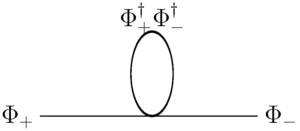
Figure 1: Superfield diagram for proper self-energy $\Sigma_{+-}(p,\theta^{2})$ with the dimension six four-superfield interaction.

 

A couple of remarks are in order. Firstly, if the parameter $\tilde{m}_{\!\scriptscriptstyle C}^{2}$ vanishes, we have $\eta=0$ and hence the gap equation for $m$ reduces to

$$m=2m\,g^{2}I(|m|^{2},\tilde{m}^{2},\Lambda^{2})\;,$$ (17)

where

$$I(|m|^{2},\tilde{m}^{2},\Lambda^{2})=\frac{1}{16\pi^{2}}\left[|m|^{2}\ln{\frac{|m|^{2}(|m|^{2}+\tilde{m}^{2}+\Lambda^{2})}{(|m|^{2}+\tilde{m}^{2})(|m|^{2}+\Lambda^{2})}}+\tilde{m}^{2}\ln\left(1+\frac{\Lambda^{2}}{|m|^{2}+\tilde{m}^{2}}\right)\right]\;.$$ (18)

The equation gives a supersymmetric Dirac mass $m$ which vanishes for $\tilde{m}^{2}=0$. Note that the case with both $\tilde{m}_{\!\scriptscriptstyle C}^{2}$ and $\tilde{m}^{2}$ being zero corresponds to the SNJL model with an exactly supersymmetric Lagrangian BL . On the other hand, taking the limit $\tilde{m}\rightarrow\infty$ where the scalar particles of $\Phi_{\pm}$ become heavy and decoupled, $m$ becomes the simple Dirac fermion/quark mass which then satisfies the equation

$$m=\frac{mg^{2}}{8\pi^{2}}\big{[}\Lambda^{2}+|m|^{2}\ln{|m|^{2}}-|m|^{2}\ln(\Lambda^{2}+|m|^{2})\big{]}\;,$$ (19)

giving

$$(g^{2})^{-1}=\frac{\Lambda^{2}}{8\pi^{2}}\left[1-\frac{|m|^{2}}{\Lambda^{2}}\,\ln{\frac{\Lambda^{2}}{|m|^{2}}}+O(1/\Lambda^{4})\right]\;.$$ (20)

This is the standard NJL result for the pure fermionic model usually given with and extra $N_{c}$ factor for the $\psi_{\pm}$ fermions as colored quarks. For the SNJL case with nonzero $\tilde{m}^{2}$, the gap equation for $m$ has been obtained in Ref.BE through a component field effective potential analysis of the low energy effective Lagrangian after the introduction of two auxiliary (Higgs/composite) superfields. Their result is

$$\frac{2mg}{\Lambda^{2}}\left[\frac{8\pi^{2}}{g^{2}\Lambda^{2}}-\frac{|m|^{2}+\tilde{m}^{2}}{\Lambda^{2}}\ln\left(1+\frac{\Lambda^{2}}{|m|^{2}+\tilde{m}^{2}}\right)+\frac{|m|^{2}}{\Lambda^{2}}\ln\left(1+{\frac{\Lambda^{2}}{|m|^{2}}}\right)\right]=0\;.$$ (21)

One can easily see, with a little algebra, that it agrees exactly with our result. Note that nontrivial solution for $m$ exists for the coupling constant satisfying the inequality BE

$$g^{2}>\frac{8\pi^{2}}{\tilde{m}^{2}\ln\left(1+\frac{\Lambda^{2}}{\tilde{m}^{2}}\right)}\;,$$ (22)

generating a mass for the Dirac fermion pair. As we will also illustrate in the next section, the mass term comes from a bi-superfield condensate, which contains a bi-fermion part, that breaks the chiral symmetry in the original Lagrangian.

The case without supersymmetry breaking corresponds to $\tilde{m}^{2}=\tilde{m}_{\!\scriptscriptstyle C}^{2}=0$. In that case, a supergraph analysis has been performed going to two-loop evaluation of $\Sigma^{({\mbox{\tiny}loop})}_{+-}(p,\theta)$ BL . No nontrivial solution for $m$ exists. While we do not have serious doubt on that result, we note that their superfield gap equation analysis did not include the equation for $\eta$, the supersymmetric breaking part, as we do. Our result here, however, explicitly establishes that, up to the one-loop level, vanishing $\tilde{m}_{\!\scriptscriptstyle C}^{2}$ necessarily implies zero $\eta$ no matter what value $\tilde{m}^{2}$ has. Formally speaking, such fully general gap equation result still have to be obtained for the two-loop analysis; and nontrivial solution for $\eta$ will imply spontaneous supersymmetry breaking.

To further illustrate the power of our general gap equation results, we report also result for a scenario on the other extreme where $m=0$ but $\eta\neq 0$ solution for Eq.(16). Naively, one enforces zero $m$ in the the $I_{2}$ integral of the equation for $\eta$. Nontrivial solution for the latter exists under the condition

$$\frac{1}{16\pi^{2}}\left[\ln{\left(1+\frac{\Lambda^{2}}{\tilde{m}^{2}}\right)}-\frac{\Lambda^{2}}{\Lambda^{2}+\tilde{m}^{2}}\right]\leq\frac{1}{-g^{2}\tilde{m}_{\!\scriptscriptstyle C}^{2}}<\frac{1}{16\pi^{2}}\ln{\left(1+\frac{\Lambda^{2}}{2\tilde{m}^{2}}\right)}\;,$$ (23)

details of the analysis behind which we leave to appendix A. The last part of the inequality comes from an analysis similar to that of the condition for nonotrivial $m$ under $\eta=0$. The magnitude of the responsible coupling, ${g^{2}\tilde{m}_{\!\scriptscriptstyle C}^{2}}$ here, has to be big enough. The other part of the inequality is actually from $|\eta|\leq(m^{2}+\tilde{m}^{2})$ beyond which there will be a tachyonic scalar mass eigenvalue. Note that one always needs a negative ${\tilde{m}_{\!\scriptscriptstyle C}^{2}}$ for nontrivial $\eta$ solution. The parameter is to be appreciated as the soft mass term for the composite superfield, as we will show explicitly in the next section.

Next we turn to the dimension five holomorphic interaction case, which actually shows an amazingly strong interplay between $m$ and $\eta$.

II.2 Results from the dimension five interaction

For the dimension five interaction, the G vertex gives at one-loop level a diagram only slightly different from the previous case, as Fig. 2. The propagator $\Phi_{+}\Phi_{-}$ is involved instead. Again, we write schematically

$$\Sigma^{({\mbox{\tiny}fig2})}=\Sigma^{({\mbox{\tiny}fig2})}_{1}+\Sigma^{({\mbox{\tiny}fig2})}_{2a}+\Sigma^{({\mbox{\tiny}fig2})}_{2b}+\Sigma^{({\mbox{\tiny}fig2})}_{3a}+\Sigma^{({\mbox{\tiny}fig2})}_{3b}\;.$$

Our calculations give the partial amplitude from the various parts of the propagator in Eq.(9) as

$$\int\!\!d^{2}\!\bar{\theta}\,\Sigma^{({\mbox{\tiny}{fig2}})}_{1}\,\delta^{2}\!(\bar{\theta}) = \int\!\!d^{2}\!\bar{\theta}\,0\,\delta^{2}\!(\bar{\theta})\;,$$

$$\int\!\!d^{2}\!\bar{\theta}\,\Sigma^{({\mbox{\tiny}{fig2}})}_{2a}\,\delta^{2}\!(\bar{\theta}) = \int\!\!d^{2}\!\bar{\theta}\,\,\frac{\bar{\eta}G}{2}(1+B\theta^{2})\,I_{2}(|m|^{2},\tilde{m}^{2},|\eta|,\Lambda^{2})\,\delta^{2}\!(\bar{\theta})\;,$$

$$\int\!\!d^{2}\!\bar{\theta}\,\Sigma^{({\mbox{\tiny}{fig2}})}_{2b}\,\delta^{2}\!(\bar{\theta}) = \int\!\!d^{2}\!\bar{\theta}\,0\,\delta^{2}\!(\bar{\theta})\;,$$

$$\int\!\!d^{2}\!\bar{\theta}\,\Sigma^{({\mbox{\tiny}{fig2}})}_{3a}\,\delta^{2}\!(\bar{\theta}) = \int\!\!d^{2}\!\bar{\theta}\,\frac{-\bar{m}G}{2}(1+B\theta^{2})\,I_{1}(|m|^{2},\tilde{m}^{2},|\eta|,\Lambda^{2})\,{\theta}^{2}\,\delta^{2}\!(\bar{\theta})\;,$$

$$\int\!\!d^{2}\!\bar{\theta}\,\Sigma^{({\mbox{\tiny}{fig2}})}_{3b}\,\delta^{2}\!(\bar{\theta}) = \int\!\!d^{2}\!\bar{\theta}\,\frac{-\bar{m}G}{2}(1+B\theta^{2})\,I_{1}(|m|^{2},\tilde{m}^{2},|\eta|,\Lambda^{2})\,{\theta}^{2}\,\delta^{2}\!(\bar{\theta})\;.$$ (24)

where $I_{1}(|m|^{2},\tilde{m}^{2},|\eta|,\Lambda^{2})$ and $I_{2}(|m|^{2},\tilde{m}^{2},|\eta|,\Lambda^{2})$ are the same loop integrals as in Eq.(15). That gives the gap equation with $\Sigma^{({\mbox{\tiny}{fig2}})}$ as

$$m = \frac{\bar{\eta}G}{2}\;I_{2}(|m|^{2},\tilde{m}^{2},|\eta|,\Lambda^{2})\;,$$

$$\eta = \bar{m}G\;I_{1}(|m|^{2},\tilde{m}^{2},|\eta|,\Lambda^{2})-\frac{\bar{\eta}GB}{2}\;I_{2}(|m|^{2},\tilde{m}^{2},|\eta|,\Lambda^{2})\;.$$ (25)

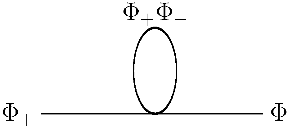
Figure 2: Superfield diagram for proper self-energy $\Sigma_{+-}(p,\theta^{2})$ with the dimension five four-superfield interaction.

 

The first thing to note in the gap equation result is the important fact that the equations for $m$ and $\eta$ are completely coupled. If one naively drop $\eta$ from consideration, for instance, one will not see any nontrivial expression and completely miss the possible dynamical mass generation. The two parameters will either both have nontrivial solutions or both vanishing.

Considering only the case of real values for $m$ and $\eta$ under the assumption of a real and small $B$ value, we find that nontrivial solution exists for large enough G (taken as real and positive here by convention) satisfying

$$G>\sqrt{G_{0}^{2}+b^{2}}+b\sim G_{0}+b\;,$$ (26)

where

$$G_{0}^{2}=\frac{512\pi^{2}}{\tilde{m}^{2}\ln{\left(1+\frac{\Lambda^{2}}{\tilde{m}^{2}}\right)}\left[\ln{\left(1+\frac{\Lambda^{2}}{\tilde{m}^{2}}\right)}-\frac{\Lambda^{2}}{\tilde{m}^{2}+\Lambda^{2}}\right]}\;$$ (27)

gives the critical $G^{2}$ for $B=0$, and

$$b=B\;\frac{8\pi^{2}}{\tilde{m}^{2}\ln{\left(1+\frac{\Lambda^{2}}{\tilde{m}^{2}}\right)}}\;.$$ (28)

Details are to be given in appendix A. Note that $B$ may be positive or negative, or more generally contains a complex phase. Solution condition for more general cases is to be further investigated.

III Model Features of Mass Generation and Symmetry Breaking

Let us take a careful look at the mass generation and symmetry breaking structure of the two simplest models with the different four-superfield interactions. That is best done in each case with the consideration of the effective theory having the composite superfield as a basic ingredient. We will see that the HSNJL model has theoretical features at least as appealing as the NJL model itself, while the SNJL model maybe considered somewhat inferior in comparison. The model also raises the idea of bi-scalar condensate playing a key role in (fermion) mass generation and symmetry breaking.

In our HSNJL model with the dimension five four-superfield interaction 034 , the bi-superfield condensate $\left\langle\Phi_{+}\Phi_{-}\right\rangle$ is considered to be the source of mass generation. Hence, whatever symmetry the superfield product carries a nontrivial quantum number will be spontaneously broken through the dynamics. The symmetry breaking vacuum condensate can have a supersymmetric part and a supersymmetry breaking part. One can see easily that the condensate induces mass term ${\mathcal{M}}$ by explicitly matching expression (11) to the term as

$$-\frac{G}{2}\int\!\!d^{2}\!\theta\,\left\langle\Phi_{+}\Phi_{-}\right\rangle\Phi_{+}\Phi_{-}\,(1+B\theta^{2})\longrightarrow\int\!\!d^{2}\!\theta\,(m-\eta\,\theta^{2})\,\Phi_{+}\Phi_{-}\;,$$

which gives

$$m\;(\Phi_{+}\Phi_{-})_{F} = -\,G\left\langle\Phi_{+}\Phi_{-}\right\rangle_{A}\,(\Phi_{+}\Phi_{-})_{F}\;,$$

$$\eta\;(\Phi_{+}\Phi_{-})_{A} = G\bigg{(}\left\langle\Phi_{+}\Phi_{-}\right\rangle_{F}+B\left\langle\Phi_{+}\Phi_{-}\right\rangle_{A}\bigg{)}(\Phi_{+}\Phi_{-})_{A}\;.$$ (29)

The supersymmetry breaking nature of $\eta$ is clearly illustrated in the last equation. It is really a contribution to the so-called left-right mixing of the scalar mass. It has already been pointed out that the model has the bi-superfield condensate $\left\langle\Phi_{+}\Phi_{-}\right\rangle_{F}$ [which contains a bi-fermion part : $(\Phi_{+}\Phi_{-})_{F}=A_{+}F_{-}+F_{+}A_{-}-\psi_{+}\psi_{-}$] contributing only to scalar mass (mixing) while it is the bi-scalar condensate $\left\langle\Phi_{+}\Phi_{-}\right\rangle_{A}$ that gives Dirac fermion mass 035 . Recall that the model actually has no four-fermion interaction, unlike the case of the SNJL model.

In the SNJL model with the dimension six four-superfield interaction, however, the story is less straightforward. The interaction term from expression (10) in the presence of the condensate $\left\langle\Phi_{+}\Phi_{-}\right\rangle$ reads

$$g^{2}\int\!\!d^{4}\theta\,\left\langle\Phi_{+}^{\dagger}\Phi_{-}^{\dagger}\right\rangle\Phi_{+}\Phi_{-}\,(1-\tilde{m}_{\!\scriptscriptstyle C}^{2}\theta^{2}{\bar{\theta}}^{2})\;.$$

The component content is given by

$$g^{2}\left\langle\Phi_{+}^{\dagger}\Phi_{-}^{\dagger}\right\rangle_{\!F}\,(\Phi_{+}\Phi_{-})_{F}\qquad\mbox{and}\qquad-g^{2}\tilde{m}_{\!\scriptscriptstyle C}^{2}\,\left\langle\Phi_{+}^{\dagger}\Phi_{-}^{\dagger}\right\rangle_{\!A}\,(\Phi_{+}\Phi_{-})_{A}\;.$$

For the two terms to be recast as components of a superfield Dirac mass term ${\mathcal{M}}$, we have

$$m = g^{2}\left\langle\Phi_{+}^{\dagger}\Phi_{-}^{\dagger}\right\rangle_{\!F}\;,$$

$$\eta = g^{2}\tilde{m}_{\!\scriptscriptstyle C}^{2}\,\left\langle\Phi_{+}^{\dagger}\Phi_{-}^{\dagger}\right\rangle_{\!A}\;.$$ (30)

The matching of $\left\langle\Phi_{+}^{\dagger}\Phi_{-}^{\dagger}\right\rangle$ to ${\mathcal{M}}$ is hence in the wrong order, with a switching of the scalar $A$- and auxiliary $F$- parts. Only through the introduction of an auxiliary Higgs superfield $\Phi_{\!\scriptscriptstyle H}$ other than the $\Phi_{+}\Phi_{-}$ composite one can put the term originated in the Kähler potential as a superpotential term. This twisting of matching the dimension six Kähler potential term to a superpotential term as the Dirac mass is the reason why one cannot take the $\Phi_{+}\Phi_{-}$ composite to be an effective Higgs superfield directly BE — a price to pay to retain a four-fermion interaction.

The very different theoretical structure between the two models will be more transparent with the effective theory perspective. For the HSNJL model, we have 034

$${\cal L}_{\mbox{\tiny HSNJL}}^{\mbox{\tiny eff}} = \int\!d^{4}\theta\left({\Phi}_{+}^{\dagger}{\Phi}_{+}+{\Phi}_{-}^{\dagger}{\Phi}_{-}\right)(1-\tilde{m}^{2}\theta^{2}\bar{\theta}^{2})$$ (31)

$$+\left\{\int\!d^{2}\!\theta\left[\frac{1}{2}(\sqrt{\mu_{0}}{\Phi}_{0}+\sqrt{G}{\Phi}_{+}{\Phi}_{-})(\sqrt{\mu_{0}}{\Phi}_{0}+\sqrt{G}{\Phi}_{+}{\Phi}_{-})\right.\right.$$

$$\left.\left.\qquad-\frac{G}{2}{\Phi}_{+}{\Phi}_{-}{\Phi}_{+}{\Phi}_{-}\right](1+B\theta^{2})+h.c.\right\}$$

$$= \int d^{4}\theta\left({\Phi}_{+}^{\dagger}{\Phi}_{+}+{\Phi}_{-}^{\dagger}{\Phi}_{-}\right)(1-\tilde{m}^{2}\theta^{2}\bar{\theta}^{2})$$

$$+\left\{\int\!d^{2}\!\theta\left[\frac{\mu_{0}}{2}{\Phi}_{0}^{2}+\sqrt{\mu_{0}G}{\Phi}_{0}{\Phi}_{+}{\Phi}_{-}\right](1+B\theta^{2})+h.c.\right\}\;,$$

where ${\Phi}_{0}$ is the auxiliary Higgs superfield that comes out as the composite

$${\Phi}_{0}=-\sqrt{G/\mu_{0}}\,{\Phi}_{+}{\Phi}_{-}\;,$$ (32)

from its own equation of motion. Hence, the Lagrangian differs from the original one only in having an extra term that vanished by the above equation. The path integral over the auxiliary superfield is a trivial Gaussian. When it is integrated out in the effective theory, one can retrieve the generating functional of the original theory up to a constant factor. This feature mimics exactly that of the NJL modelKK . As the ${\Phi}_{0}$ develops a vacuum expection value (VEV), we have the mass

$${\mathcal{M}}=m-\eta\theta^{2}=\sqrt{\mu_{0}G}\left\langle{\Phi}_{0}\right\rangle(1+B\theta^{2})$$ (33)

or

$$m = \sqrt{\mu_{0}G}\left\langle{\Phi}_{0}\right\rangle_{A}\;,$$

$$\eta = -\sqrt{\mu_{0}G}\left(\,\left\langle{\Phi}_{0}\right\rangle_{F}+B\left\langle{\Phi}_{0}\right\rangle_{A}\right)\;.$$ (34)

The result matches directly to that of Eq.(29), again mimicking exactly the basic feature in the NJL model. Despite having a four-superfield interaction that does not contain a four-fermion interaction, the HSNJL model with its effective Lagrangian formulation looks like an exact supersymmetrization of the NJL model.

Situation for the case of the SNJL model is quite a bit more complicated. In the effective theory picture, the Higgs superfield cannot be obtained as the composite. We have instead

$${\cal L}_{\mbox{\tiny SNJL}}^{\mbox{\tiny eff}} = \int d^{4}\theta\left[\left({\Phi}_{+}^{\dagger}{\Phi}_{+}+{\Phi}_{-}^{\dagger}{\Phi}_{-}\right)(1-\tilde{m}^{2}\theta^{2}\bar{\theta}^{2})+{\Phi}_{\!\scriptscriptstyle C}^{\dagger}{\Phi}_{\!\scriptscriptstyle C}\,(1-\tilde{m}_{\!\scriptscriptstyle C}^{2}\theta^{2}{\bar{\theta}}^{2})\right]$$ (35)

$$+\left\{\int\!d^{2}\!\theta\;\mu\;{\Phi}_{\!\scriptscriptstyle H}\left({\Phi}_{\!\scriptscriptstyle C}+g\Phi_{+}\Phi_{-}\right)(1+A\theta^{2})+h.c.\right\}\;.$$

where ${\Phi}_{\!\scriptscriptstyle H}$ is the auxiliary Higgs superfield whose equation of motion gives the other superfield introduced ${\Phi}_{\!\scriptscriptstyle C}$ as the composite

$${\Phi}_{\!\scriptscriptstyle C}=-{g}\Phi_{+}\Phi_{-}\;.$$ (36)

In addition, we have put in an extra supersymmetry breaking part characterized by parameter $A$ in the superpotential. Unlike the $B$ parameter in the previous model, the admissible $A$ parameter is arbitrary; it is not even related to any parameter in the original Lagrangian. Apart from adding to the original Lagrangian the superpotential term which is constrained to be zero, we actually have to replace the $g^{2}{\Phi}_{+}^{\dagger}{\Phi}_{-}^{\dagger}{\Phi}_{+}{\Phi}_{-}$ in the Kähler potential by ${\Phi}_{\!\scriptscriptstyle C}^{\dagger}{\Phi}_{\!\scriptscriptstyle C}$ too. Moreover, from the point of view of the original Lagrangian, there is no clear picture on how the ${\Phi}_{\!\scriptscriptstyle H}$, or rather $\mu{\Phi}_{\!\scriptscriptstyle H}$, arises out of the dynamics for ${\Phi}_{\pm}$. It is not a simple composite. Equations of motion for components of ${\Phi}_{\!\scriptscriptstyle C}$ from the effective Lagrangian give, for instance,

$$\mu F_{\scriptscriptstyle H}+A\,\mu A_{\scriptscriptstyle H} = -\partial^{m}\partial_{m}A_{\scriptscriptstyle C}^{*}-\tilde{m}_{\!\scriptscriptstyle C}^{2}\,A_{\scriptscriptstyle C}^{*}\;,$$

$$\mu\psi_{\scriptscriptstyle H} = -i\sigma^{m}\partial_{m}\psi_{\scriptscriptstyle C}^{\dagger}\;,$$

$$\mu A_{\scriptscriptstyle H} = -F_{\scriptscriptstyle C}^{*}\;,$$ (37)

respectively. Nevertheless, the Lagrangian in the presence of nontrivial VEV for ${\Phi}_{\!\scriptscriptstyle H}$ gives

$${\mathcal{M}}=m-\eta\,\theta^{2}={\mu g}\left\langle{\Phi}_{\!\scriptscriptstyle H}\right\rangle(1+A\theta^{2})\;.$$ (38)

The result needs to be mapped to that of Eq.(30) as

$$m = {\mu g}\left\langle{\Phi}_{\!\scriptscriptstyle H}\right\rangle_{A}\quad\longrightarrow\quad-{g}\left\langle{\Phi}_{\!\scriptscriptstyle C}^{\dagger}\right\rangle_{F}\;,$$

$$\eta = -{\mu g}\left(\,\left\langle{\Phi}_{\!\scriptscriptstyle H}\right\rangle_{F}+A\left\langle{\Phi}_{\!\scriptscriptstyle H}\right\rangle_{A}\right)\quad\longrightarrow\quad-{g}\,\tilde{m}_{\!\scriptscriptstyle C}^{2}\left\langle{\Phi}_{\!\scriptscriptstyle C}^{\dagger}\right\rangle_{A}\;.$$ (39)

The matching is consistent with Eq.(37). Contrary to a claim in Ref.92 , we see that nonzero $\eta$ and hence nonzero $\left\langle{\Phi}_{\!\scriptscriptstyle C}^{\dagger}\right\rangle_{A}$ is possible even with $A=0$. As mentioned above, the $A$ parameter has no role in the original Lagrangian. Actually, Eq.(37) also shows the parameter is not constrained, while its value affects the determination of the auxiliary component of ${\Phi}_{\!\scriptscriptstyle H}$.

We can see from above the ${\Phi}_{\!\scriptscriptstyle 0}$ and ${\Phi}_{\!\scriptscriptstyle C}$ as superfield composites have the quantum number of $\Phi_{+}\Phi_{-}$, while ${\Phi}_{\!\scriptscriptstyle H}$ has the conjugate quantum number. With the mass term generated, the two chiral superfields $\Phi_{+}$ and $\Phi_{-}$ make a Dirac pair. The simplest symmetry breaking picture of the SNJL model, for singlet superfields, is that of the Dirac fermion chiral symmetry, namely $U(1)_{V}\times U(1)_{A}\rightarrow U(1)_{V}$, which is the same as the original NJL model. The Standard Model with spontaneous electroweak symmetry breaking, however, has Weyl fermions as a basic ingredient with gauge symmetry forbidding any Dirac pairing. It is the same in theories with (N=1) supersymmetry. Chiral superfields are chiral exactly because they bear each a Weyl fermion. With such theories, chiral symmetry is not an issue. The $U(1)_{V}\times U(1)_{A}$ symmetry is really a $U(1)_{+}\times U(1)_{-}$, or $\Phi_{+}$ and $\Phi_{-}$ number symmetries which one has no reason to expect an interaction term to respect. It is broken by the dimension five interaction in the HSNJL model. The SNJL model breaks the $U(1)_{+}\times U(1)_{-}$ symmetry dynamically to a $U(1)_{+}-U(1)_{-}$ symmetry.

In the simplest model with the holomorphic four-superfield interaction discussed above, presence of the ${\Phi}_{\!\scriptscriptstyle 0}^{2}$ term says that composite ${\Phi}_{\!\scriptscriptstyle 0}$ has to be in the real representation of the model symmetry. Symmetry breaking options are hence very limited. In a model with more than two basic chiral superfields (superfields $\Phi_{+}$ and/or $\Phi_{-}$ being multiplets), a holomorphic four-superfield interaction may give rise to a wide range of symmetry breaking. We focus in this paper in the simplest model of the type, to illustrate the basic feature. To give an explicit symmetry breaking picture for the simplest version of the HSNJL model (with singlet superfields), one can consider a $Z_{4}$ symmetry under which both the $\Phi_{+}$ and $\Phi_{-}$ superfields have a basic charge $e^{i\pi/2}$. The dimension five interaction obviously respects the symmetry while the $\Phi_{+}\Phi_{-}$ Dirac mass term is not allowed, that is till the $Z_{4}$ symmetry is dynamically broken by the $\Phi_{+}\Phi_{-}$ vacuum condensate. The condensate leaves a $Z_{2}$ symmetry that survives. An $SU(2)$ symmetry breaking example can be constructed with $\Phi_{+}$ being an $SU(2)$-triplet while having an equal and opposite $U(1)$ charge with a singlet $\Phi_{-}$. The $\Phi_{+}\Phi_{-}$ term is then invariant under the $U(1)$ but remains an $SU(2)$-triplet; its condensate breaks the $SU(2)$ symmetry. In that case, the condensate will be along one of the three $SU(2)$ components. Hence the Dirac mass is only for the corresponding component of $\Phi_{+}$ which is what really forms a Dirac pair with the singlet $\Phi_{-}$. The other two components of the $\Phi_{+}$ multiplet remains massless. Note that an explicit model giving rise to electroweak symmetry breaking in an effective supersymmetric standard model has been discussed in Ref.034 . The model involves three superfield multiplets with two superfield condensates but otherwise the same holomorphic four-superfield interaction structure. We will give more details for the continuous symmetry cases in appendix B.

IV Conclusion

We presented above derivation of the superfield gap equations for the simplest models with a dimension six or dimension five four-superfield interactions, and analyzed some interesting cases for nontrivial solution. We proposed that the gap equation in the superfield setting should be taken as one on the Dirac mass parameter as a superspace scalar, like a constant superfield, with both a supersymmetric and a supersymmetry breaking part. The amplitude of the proper self-energy diagram, or two-point functions, effective action $\dots$ etc., should all be considered in the same footing. Of course the fermionic part should be zero. The supersymmetric breaking auxiliary part, however, is in general nontrivial and could have an important role to play. From our results for the Dirac mass parameter $\mathcal{M}=m-\theta^{2}\eta$ in the case of the dimension five interaction, nontrivial solution for $m$ requires nonzero $\eta$, and vice versa. Considering the usual supersymmetric Dirac mass $m$ only will completely miss the result. For the dimension six case, though independent nontrivial solution for $m$ and $\eta$ are possible, a nontrivial $\eta$ has its own interest and does affect the solution for $m$. The approach will also be useful to check spontaneous supersymmetry breaking.

The two kinds of four-superfield interactions are alternative supersymmetrization of the four-fermion interaction in the NJL model of dynamical mass generation and symmetry breaking. They could each be used as a mechanism for dynamical electroweak symmetry breaking. The two kinds of models (SNJL and HSNJL models) have otherwise very different theoretical mass generation features, with phenomenological implications. We illustrated some of the key aspects.

Our results explicitly establish the dynamical mass generation induced by the dimension five four-superfield interaction, for the prototype HSNJL model. The model has actually no four-fermion interaction and has a bi-scalar condensate, instead of bi-fermion condensate, as the source of Dirac fermion mass. It has otherwise theoretical features that look like a direct supersymmetric version of the NJL model. It is arguably a more natural supersymmetrization of the latter, though only constructed almost thirty years after the SNJL model with the four-fermion interaction. It is expected to provide an alternative paradigm for dynamical mass generation and symmetry breaking, at least for superfield theories. The explicit symmetry breaking picture of the simplest HSNJL model maybe considered as $Z_{4}\rightarrow Z_{2}$. A version of the HSNJL with the basics superfields being (gauge) multiplets gives a simple application to the breaking of a continuous symmetry. A simple example is given by an $SU(2)\times U(1)$ triplet and a singlet. We also have extended versions with more than two basic superfield multiplets that can achieve a rich spectrum of dynamical symmetry breaking. A case example, which was also the original target for the idea of the HSNJL model is the one for electroweak symmetry breaking. More details are available in appendix B.

Appendix A Analysis of Conditions for Nontrivial Solutions of the Gap Equations

We have two pairs of gap equations,

$$m = 2mg^{2}I_{1}(|m|^{2},\tilde{m}^{2},|\eta|,\Lambda^{2})\;,$$

$$\eta = -\eta\,g^{2}\tilde{m}_{\!\scriptscriptstyle C}^{2}\,{I}_{2}(|m|^{2},\tilde{m}^{2},|\eta|,\Lambda^{2})\;,$$ (40)

for the case of a dimension six interaction, and

$$m = \frac{\bar{\eta}G}{2}\;I_{2}(|m|^{2},\tilde{m}^{2},|\eta|,\Lambda^{2})\;,$$

$$\eta = \bar{m}G\;I_{1}(|m|^{2},\tilde{m}^{2},|\eta|,\Lambda^{2})-\frac{\bar{\eta}GB}{2}\;I_{2}(|m|^{2},\tilde{m}^{2},|\eta|,\Lambda^{2})\;,$$ (41)

for the case of the dimension five interaction.

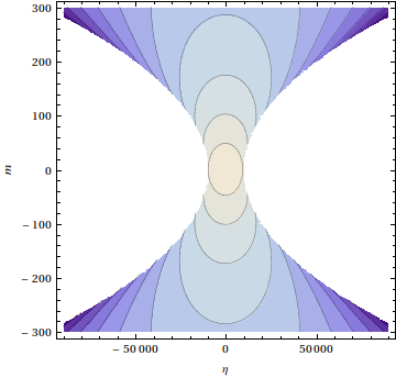
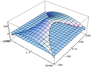
Figure 3: Contour plot (left) and 3D plot (right) of $I_{1}$ in the real $\left(\eta,m\right)$ plane.

 

We first look into the general properties of the two loop-functions $I_{1}$ and $I_{2}$. The shape of function $I_{1}$ is presented in Fig. 3 for generic given $\Lambda$ and $\tilde{m}^{2}$. Here we consider only real values for $m$ and $\eta$. The blank regions are where $|\eta|>m^{2}+\tilde{m}^{2}$, which gives an unacceptable tachyonic mass for a scalar mass eigenstate. We can see that the function is convex on the $\eta$-$m$ plane with its maximum value at the origin $\left(\eta=0,m=0\right)$. Along the border lines that satisfy $|\eta|=m^{2}+\tilde{m}^{2}$, the value of function approaches $-\frac{\Lambda^{2}}{32\pi^{2}}$, definitely negative. The maximum value at the origin is

$$I_{1}\left(0,\tilde{m}^{2},0,\Lambda^{2}\right)=\frac{\tilde{m}^{2}}{16\pi^{2}}\log{\left[1+\frac{\Lambda^{2}}{\tilde{m}^{2}}\right]}\;.$$ (42)

On the $\eta$-axis ($m=0$), at the both ends, i.e. $\left(|\eta|=\tilde{m}^{2},0\right)$, we have

$$I_{1}\left(0,\tilde{m}^{2},|\eta|=\tilde{m}^{2},\Lambda^{2}\right)=\frac{\tilde{m}^{2}}{16\pi^{2}}\log{\left[1+\frac{\Lambda^{2}}{2\tilde{m}^{2}}\right]}\;.$$ (43)

The $I_{2}$ function, however, has the shape of a saddle as depicted in Fig. 4. It is concave along the $\eta$-axis and convex along the $m$-axis. It attains its maximum value at $\left(|\eta|=\tilde{m}^{2},0\right)$ on the centers of the tachyonic exclusion borders ($|\eta|=m^{2}+\tilde{m}^{2}$). The value is given be

$$I_{2}\left(0,\tilde{m}^{2},|\eta|=\tilde{m}^{2},\Lambda^{2}\right)=\frac{1}{16\pi^{2}}\log{\left[1+\frac{\Lambda^{2}}{2\tilde{m}^{2}}\right]}\;.$$ (44)

The origin is a local minimum, with a value given by

$$I_{2}\left(0,\tilde{m}^{2},0,\Lambda^{2}\right)=\frac{1}{16\pi^{2}}\left(\log{\left[1+\frac{\Lambda^{2}}{\tilde{m}^{2}}\right]}-\frac{\Lambda^{2}}{\Lambda^{2}+\tilde{m}^{2}}\right)\;.$$ (45)

In addition, it is positive definite.

With the gap equation set (40), nontrivial solution for $m$ requires

$$I_{1}=\frac{1}{2g^{2}}\;,$$ (46)

hence one can easily see the lower bound for $g^{2}$ from the maximum value of $I_{1}$ given in Eq.(42). The point corresponds to $\eta=0$. For any particular nonzero $\eta$, an even larger $g^{2}$ will be required, but the simultaneous solution with

$$I_{2}=\frac{1}{-g^{2}\tilde{m}_{\!\scriptscriptstyle C}^{2}}\;,$$ (47)

is required. The latter has a negative $\tilde{m}_{\!\scriptscriptstyle C}^{2}$ as a necessary condition. The maximum value of $I_{2}$ within the no-tachyonic mass constraint given in Eq.(44) gives a lower bound for the magnitude of ${g^{2}\tilde{m}_{\!\scriptscriptstyle C}^{2}}$ and at $m=0$ the local minimum given in Eq.(45) gives an upper bound.

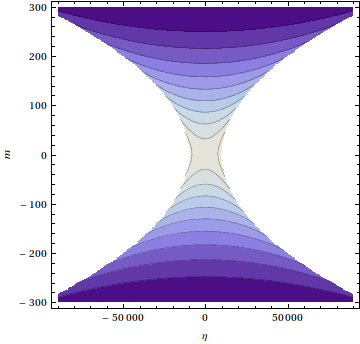
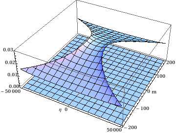
Figure 4: Contour plot (left) and 3D plot(right) of $I_{2}$ in the real $\left(\eta,m\right)$ plane.

 

With the gap equation set (41), one has to look for simultaneous nontrivial solution for $m$ and $\eta$. Without lost of generosity, one can take $G$ to be real and positive. For $B=0$, the solution satisfies the equation

$$\frac{\eta^{2}}{2}I_{2}=m^{2}I_{1}\;,$$ (48)

which is illustrated in Fig. 5 as (3) together with the two gap equations (1) and (2). The general shapes of the three curves are independent of the values of $\Lambda$ and $\tilde{m}^{2}$. We can see that so long as the slope of curve (1) at the origin is larger than that of curve (2), existence of solution as given by the intersecting points is to be expected. The slope of the curve (1) at the origin is given by

$$\frac{dm}{d\eta}_{\!\!(1)}=\frac{G}{32\pi^{2}}\left[\ln{\left(1+\frac{\Lambda^{2}}{\tilde{m}^{2}}\right)}-\frac{\Lambda^{2}}{\tilde{m}^{2}+\Lambda^{2}}\right]\;,$$ (49)

and the slope of the curve (2) is given by

$$\frac{dm}{d\eta}_{\!\!(2)}=\frac{1}{G}\frac{16\pi^{2}}{\tilde{m}^{2}\ln{\left(1+\frac{\Lambda^{2}}{\tilde{m}^{2}}\right)}}\;.$$ (50)

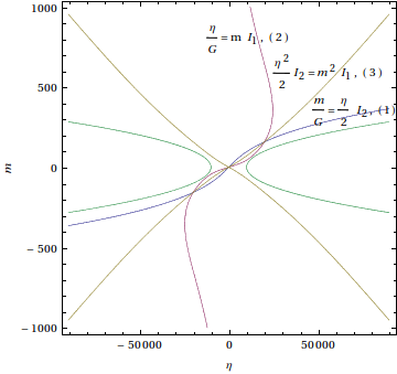
Figure 5: Solutions of to gap equations on the real $\left(\eta,m\right)$ plane.

 

Hence, the condition $\frac{dm}{d\eta}_{\!\!\scriptscriptstyle(1)}>\frac{dm}{d\eta}_{\!\!\scriptscriptstyle(2)}$ implies

$$G^{2}>G_{0}^{2}=\frac{512\pi^{2}}{\tilde{m}^{2}\ln{\left(1+\frac{\Lambda^{2}}{\tilde{m}^{2}}\right)}\left[\ln{\left(1+\frac{\Lambda^{2}}{\tilde{m}^{2}}\right)}-\frac{\Lambda^{2}}{\tilde{m}^{2}+\Lambda^{2}}\right]}\;.$$ (51)

For nonzero (real) value of $B$ small enough to be considered a perturbation for the above case, the slope of the curve (2) is modified as

$$\frac{dm}{d\eta}_{\!\!(2)}=\frac{1}{G}\frac{16\pi^{2}}{\tilde{m}^{2}\ln{\left(1+\frac{\Lambda^{2}}{\tilde{m}^{2}}\right)}}+\frac{B}{2}\frac{\left[\ln{\left(1+\frac{\Lambda^{2}}{\tilde{m}^{2}}\right)}-\frac{\Lambda^{2}}{\tilde{m}^{2}+\Lambda^{2}}\right]}{\tilde{m}^{2}\ln{\left(1+\frac{\Lambda^{2}}{\tilde{m}^{2}}\right)}}\;.$$ (52)

The condition for solution is modified to

$$G>\sqrt{G_{0}^{2}+b^{2}}+b\;,$$ (53)

where

$$b=B\;\frac{8\pi^{2}}{\tilde{m}^{2}\ln{\left(1+\frac{\Lambda^{2}}{\tilde{m}^{2}}\right)}}\;\;.$$ (54)

Appendix B Application of the models to $SU(2)\times U(1)$ symmetry breaking

We illustrate further in this appendix the application of the HSNJL and the SNJL models to the phenomenological case of electroweak symmetry breaking. The application is a key motivation for the construction of the HSNJL model reported in Ref.034 . The reference discusses the effective field theory picture, illustrates how the full Lagrangian for the MSSM can be retrieved from an original model without the Higgs superfields. The only interaction terms among the chiral superfields (besides the gauge interactions) are the dimension five superpotential terms. What is missing is the direct establishment of dynamical symmetry breaking from a first principle gap equation analysis. Hence, we perform the present study. Note that such a first principle establishment of the symmetry breaking had not been available for the SNJL model either.

To get the electroweak symmetry breaking of the MSSM, we need Higgs superfields that are $SU(2)$ doublets. A direct application of the HSNJL model only allows an effective Higgs in a real representation of the model symmetry, hence not the doublet. However, getting two Higgs doublets through a double composite/condensate structure is feasible 034 . Before going into that, let us illustrate first the single composite and single condensate case of the SJNL model and a simpler $SU(2)\times U(1)$ symmetry breaking HSNJL model we have suggested in the main text.

For the case of the SNJL model, we have the basic Lagrangian

$${\cal L} = \int\!\!d^{4}\theta\left[\hat{Q}^{\dagger}\hat{Q}(1-\tilde{m}^{2}_{Q}\theta^{2}{\bar{\theta}}^{2})+\hat{T^{c}}^{\dagger}\hat{T^{c}}(1-\tilde{m}^{2}_{t}\theta^{2}{\bar{\theta}}^{2})\right]$$ (55)

$$+ g^{2}\int\!\!d^{4}\theta\,\hat{Q}^{\dagger}\hat{T}^{c\dagger}\hat{Q}\hat{T^{c}}\,(1+\tilde{m}_{C}^{2}\theta^{2}\bar{\theta}^{2})\,.$$

The superfield notation here is the standard one in the MSSM, with $\hat{Q}$ being the quark doublet superfield (containing $t_{\scriptscriptstyle L}$ and $b_{\scriptscriptstyle L}$) and $\hat{T^{c}}$ the singlet one containing $\bar{t}$. For the superfield gap equation analysis, we add the Dirac mass term

$$\int\!\!d^{4}\theta\left[{\mathcal{M}}_{t}\,\hat{Q}\hat{T^{c}}\delta^{2}\!(\bar{\theta})+h.c.\right]\;,$$ (56)

and derive the superfield gap equation for self-consistent solutions of ${\mathcal{M}}_{t}$ with

$${\mathcal{M}}_{t}=m_{t}-{\theta}^{2}\eta_{t}\;.$$ (57)

We need, in the derivation, the (hermitian conjugate of) following propagator

$$\left\langle T(\hat{Q}(1)\hat{T^{c}}(2))\right\rangle=\frac{i\,\bar{m}_{t}}{p^{2}(p^{2}+|m_{t}|^{2})}\frac{D_{\!\scriptscriptstyle 1}^{2}}{4}\delta^{4}_{\scriptscriptstyle 12}$$ (58)

$$- \frac{i}{[(p^{2}+|m_{t}|^{2}+\frac{\tilde{m}_{Q}^{2}+\tilde{m}_{t}^{2}}{2})^{2}-\frac{1}{4}(\tilde{m}_{Q}^{2}-\tilde{m}_{t}^{2})^{2}-|\eta_{t}|^{2}]}\!\left[\frac{\bar{\eta}_{t}\,D_{\!\scriptscriptstyle 1}^{2}\bar{\theta_{\!\scriptscriptstyle 1}}^{2}}{4}-\frac{\eta_{t}|m_{t}|^{2}\,D_{\!\scriptscriptstyle 1}^{2}{\theta_{\!\scriptscriptstyle 1}}^{2}}{4p^{2}}\!\right]\!\delta^{4}_{\scriptscriptstyle 12}$$

$$+ \frac{i\,\bar{m}_{t}\;[\tilde{m}_{Q}^{2}(p^{2}+|m_{t}|^{2}+\tilde{m}_{t}^{2})-|\eta_{t}|^{2}]}{(p^{2}+|m_{t}|^{2})[(p^{2}+|m_{t}|^{2}+\frac{\tilde{m}_{Q}^{2}+\tilde{m}_{t}^{2}}{2})^{2}-\frac{1}{4}(\tilde{m}_{Q}^{2}-\tilde{m}_{t}^{2})^{2}-|\eta_{t}|^{2}]}\;\frac{D_{\!\scriptscriptstyle 1}^{2}\theta_{\!\scriptscriptstyle 1}^{2}\bar{\theta_{\!\scriptscriptstyle 1}}^{2}}{4}$$

$$+ \frac{i\,\bar{m}_{t}\;[\tilde{m}_{t}^{2}(p^{2}+|m_{t}|^{2}+\tilde{m}_{Q}^{2})-|\eta_{t}|^{2}]}{(p^{2}+|m_{t}|^{2})[(p^{2}+|m_{t}|^{2}+\frac{\tilde{m}_{Q}^{2}+\tilde{m}_{t}^{2}}{2})^{2}-\frac{1}{4}(\tilde{m}_{Q}^{2}-\tilde{m}_{t}^{2})^{2}-|\eta_{t}|^{2}]}\frac{\bar{\theta_{\!\scriptscriptstyle 1}}^{2}\theta_{\!\scriptscriptstyle 1}^{2}D_{\!\scriptscriptstyle 1}^{2}}{4}\!\delta^{4}_{\scriptscriptstyle 12}\;.$$

Note that the color indices are suppressed here, as in the Lagrangian.

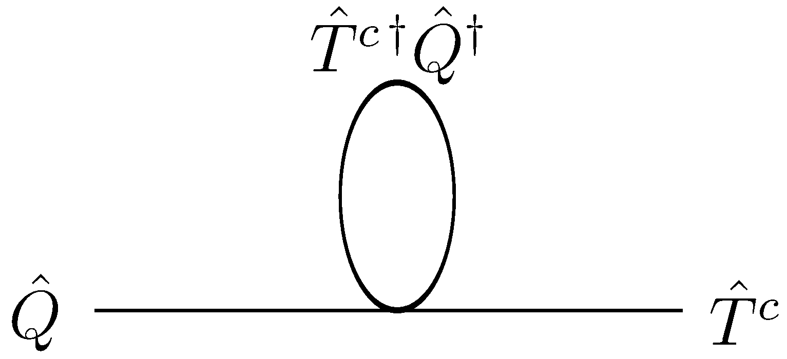
Figure 6: Superfield diagram for proper self-energy $\Sigma^{t}_{+-}(p,\theta^{2})$ with the dimension six four-superfield interaction.

 

Following the calculations as illustrated in the main text with $\Sigma^{t}_{+-}(p,\theta^{2})$ shown in Fig. 6, we have

$$m_{t} = 3\cdot 2~{}m_{t}~{}g^{2}~{}I^{\prime}_{1}(|m_{t}|^{2},\tilde{m}_{Q}^{2},\tilde{m}_{t}^{2},|\eta_{t}|,\Lambda^{2})\;,$$

$$\eta_{t} = -3~{}\eta_{t}~{}g^{2}~{}\tilde{m}_{C}^{2}~{}I^{\prime}_{2}(|m_{t}|^{2},\tilde{m}_{Q}^{2},\tilde{m}_{t}^{2},|\eta_{t}|,\Lambda^{2})\;,$$ (59)

where

$$I^{\prime}_{1}\!\left(|m_{t}|^{2},\tilde{m}_{Q}^{2},\tilde{m}_{t}^{2},|\eta_{t}|,\Lambda^{2}\right)=\!\!\int\!\!\frac{d^{4}k}{(2\pi)^{4}}\frac{[\tilde{m}_{Q}^{2}(k^{2}+|m_{t}|^{2}+\tilde{m}_{t}^{2})+\tilde{m}_{t}^{2}(k^{2}+|m_{t}|^{2}+\tilde{m}_{Q}^{2})-2|\eta_{t}|^{2}]}{(k^{2}+|m_{t}|^{2})[(k^{2}+|m_{t}|^{2}+\tilde{m}^{2})^{2}-|\eta_{t}|^{2}]}$$

$$= \frac{1}{16\pi^{2}}\left[\;\;\frac{1}{2}\left(|m_{t}|^{2}+\frac{\tilde{m}_{Q}^{2}+\tilde{m}_{t}^{2}}{2}\right)\,\ln{\frac{(|m_{t}|^{2}+\tilde{m}_{Q}^{2}+\Lambda^{2})(|m_{t}|^{2}+\tilde{m}_{t}^{2}+\Lambda^{2})-|\eta_{t}|^{2}}{(|m_{t}|^{2}+\tilde{m}_{Q}^{2})(|m_{t}|^{2}+\tilde{m}_{t}^{2})-|\eta_{t}|^{2}}}\right.$$

$$-\;|m_{t}|^{2}\ln{\frac{(|m_{t}|^{2}+\Lambda^{2})}{|m_{t}|^{2}}}\;\;+\;\sqrt{|\eta_{t}|^{2}+\frac{1}{4}(\tilde{m}_{Q}^{2}-\tilde{m}_{t}^{2})^{2}}\cdot$$

$$\left.\hskip 56.9055pt\left(\tanh^{-1}\frac{|m_{t}|^{2}+\frac{\tilde{m}_{Q}^{2}+\tilde{m}_{t}^{2}}{2}+\Lambda^{2}}{\sqrt{|\eta_{t}|^{2}+\frac{1}{4}(\tilde{m}_{Q}^{2}-\tilde{m}_{t}^{2})^{2}}}-\tanh^{-1}\frac{|m_{t}|^{2}+\frac{\tilde{m}_{Q}^{2}+\tilde{m}_{t}^{2}}{2}}{\sqrt{|\eta_{t}|^{2}+\frac{1}{4}(\tilde{m}_{Q}^{2}-\tilde{m}_{t}^{2})^{2}}}\right)\;\;\right]\;,$$

$$I^{\prime}_{2}(|m_{t}|^{2},\tilde{m}_{Q}^{2},\tilde{m}_{t}^{2},|\eta_{t}|,\Lambda^{2})=\int\frac{d^{4}k}{[(p^{2}+|m_{t}|^{2}+\frac{\tilde{m}_{Q}^{2}+\tilde{m}_{t}^{2}}{2})^{2}-\frac{1}{4}(\tilde{m}_{Q}^{2}-\tilde{m}_{t}^{2})^{2}-|\eta_{t}|^{2}]}$$

$$= \frac{1}{16\pi^{2}}\left[\frac{1}{2}\ln{\frac{(|m_{t}|^{2}+\tilde{m}_{Q}^{2}+\Lambda^{2})(|m_{t}|^{2}+\tilde{m}_{t}^{2}+\Lambda^{2})-|\eta_{t}|^{2}}{(|m_{t}|^{2}+\tilde{m}_{Q}^{2})(|m_{t}|^{2}+\tilde{m}_{t}^{2})-|\eta_{t}|^{2}}}\right.$$

$$\!\!\!\!\!+ \!\!\!\!\left.\frac{|m_{t}|^{2}+\frac{\tilde{m}_{Q}^{2}+\tilde{m}_{t}^{2}}{2}}{\sqrt{|\eta_{t}|^{2}+\frac{1}{4}(\tilde{m}_{Q}^{2}-\tilde{m}_{t}^{2})^{2}}}\left(\!\tanh^{-1}\!\frac{|m_{t}|^{2}+\frac{\tilde{m}_{Q}^{2}+\tilde{m}_{t}^{2}}{2}+\Lambda^{2}}{{\sqrt{|\eta_{t}|^{2}+\frac{1}{4}(\tilde{m}_{Q}^{2}-\tilde{m}_{t}^{2})^{2}}}}-\tanh^{-1}\frac{|m_{t}|^{2}+\frac{\tilde{m}_{Q}^{2}+\tilde{m}_{t}^{2}}{2}}{{\sqrt{|\eta_{t}|^{2}+\frac{1}{4}(\tilde{m}_{Q}^{2}-\tilde{m}_{t}^{2})^{2}}}}\right)\!\right].$$

In the gap equation, there appears extra color factor of 3. The expression corresponds otherwise exactly to the one given in the main text generalized to admit unequal soft masses for the two superfields. After all, it is standard to apply Feynman diagram calculations directly to nontrivial multiplets of any (gauge) symmetry. More explicitly, as the $\hat{Q}\hat{T^{c}}$ combination in the Dirac mass term ${\mathcal{M}}_{t}\,\hat{Q}\hat{T^{c}}$ is an $SU(2)_{L}$ doublet, the ${\mathcal{M}}_{t}$ parameter is likewise a doublet vector. The $SU(2)_{L}$ symmetry is to be applied to pick the nonzero direction of ${\mathcal{M}}_{t}$ as the symmetry breaking direction, and the corresponding matching direction in $\hat{Q}\hat{T^{c}}$ may only then be identified as the $t_{\scriptscriptstyle L}$ direction. With the direction assumed, the gap equation is one for a superfield scalar parameter ${\mathcal{M}}_{t}$.

There is a simple, special, case for which it is easy to see that the gap equation does admit nontrivial electroweak symmetry breaking solution. If we take $\tilde{m}_{Q}^{2}=\tilde{m}_{t}^{2}$ in the Lagrangian of Eqn.(62), the case is essentially the same as the one analyzed in the main text. Explicitly, the integrals reduce exactly to the ones given there; and with the color factor 3 absorbed into $g^{2}$ the gap equation becomes identical to the one analyzed. Hence, electroweak symmetry breaking is established for the SNJL model. For the more general $\tilde{m}_{Q}^{2}\neq\tilde{m}_{t}^{2}$ case, solution analysis similar to the one for the prototype case presented in the main text can be performed. One may also consider modifying effects from a fully realistic Lagrangian, for example from the QCD interaction. That is, however, beyond the scope of the present paper.

Next, we take on the one composite/condensate HSNJL model with $SU(2)\times U(1)$ symmetry suggested in the main text. This is a model with $\Phi_{+}\equiv\Phi_{3_{+}}$, an $SU(2)$ triplet with an $U(1)$ charge, and $\Phi_{-}\equiv\Phi_{1_{-}}$, an $SU(2)$ singlet with the opposite $U(1)$ charge. We have, explicitly, the Lagrangian

$${\cal L}= \int\!\!d^{4}\theta~{}\bigg{[}\left(\Phi_{3_{+}}^{\dagger}\Phi_{3_{+}}+\Phi_{1_{-}}^{\dagger}\Phi_{1_{-}}\right)(1-\tilde{m}^{2}\theta^{2}{\bar{\theta}}^{2})\bigg{]}$$ (61)

$$- \frac{G}{2}\int\!\!d^{4}\theta\left(\Phi_{3_{+}}\Phi_{1_{-}}\right)^{2}\,\delta^{2}\!(\bar{\theta})+h.c.\;,$$

in which we stick to the universal soft supersymmetry breaking mass term for simplicity. By introducing the mass term ${\cal M}\Phi_{3_{+}}\Phi_{1_{-}}$, with ${\cal M}=m-\theta^{2}\eta$ as in the main text, the supergraph calculation and resulted gap equation as derived from the diagram in Fig. 7 are exactly those given in the main text. Again, the Dirac mass ${\cal M}$ is naively an $SU(2)$ triplet vector in which one direction would be single out by the symmetry breaking. Hence, our analysis in the main text leads to the conclusion that the HSNJL model has $SU(2)\times U(1)$ symmetry breaking solutions. The model can be extended to have the symmetry as a gauge one. It may be consider a prototype model of continuous (gauge) symmetry breaking with the dimension five four-superfield interaction. However, the composite superfield $\Phi_{3_{+}}\Phi_{1_{-}}$ developing vacuum condensate is an $SU(2)$ triplet with zero charge under the $U(1)$, hence not one that can be used for the phenomenological electroweak symmetry breaking.

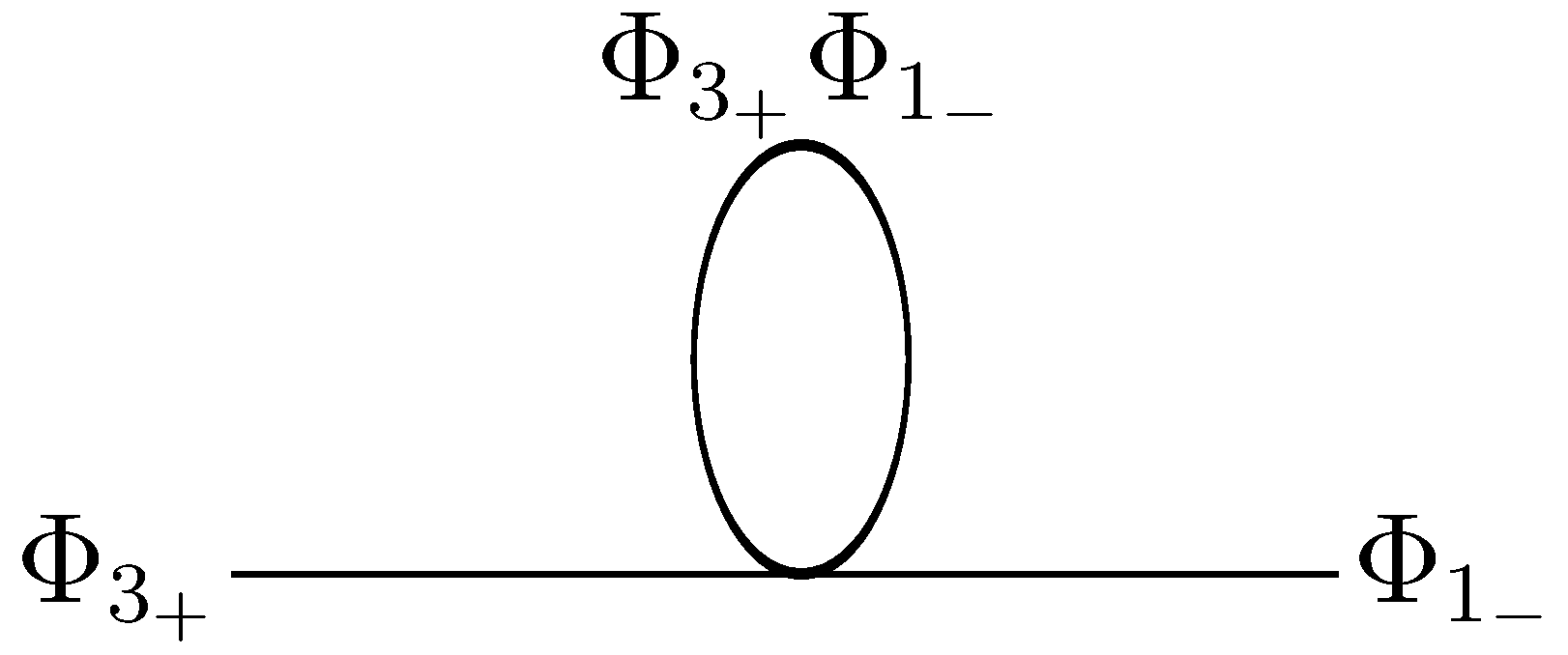
Figure 7: Superfield diagram for proper self-energy $\Sigma_{+-}(p,\theta^{2})$ with the dimension five four-superfield interaction involving a triplet and a singlet.

 

The HSNJL case to be applied to the MSSM is a bit more complicated. The basic Lagrangian is

$${\cal L} = \int\!\!d^{4}\theta~{}\left[\hat{Q}^{\dagger}\hat{Q}(1-\tilde{m}^{2}_{Q}\theta^{2}{\bar{\theta}}^{2})+\hat{T^{c}}^{\dagger}\hat{T^{c}}(1-\tilde{m}^{2}_{t}\theta^{2}{\bar{\theta}}^{2})+\hat{B}^{c\!^{\dagger}}\hat{B^{c}}(1-\tilde{m}^{2}_{b}\theta^{2}{\bar{\theta}}^{2})\right]$$ (62)

$$- \frac{G}{2}\int\!\!d^{4}\theta\,\hat{Q}\hat{T^{c}}\hat{Q}\hat{B^{c}}\,(1+B\theta^{2})\,\delta^{2}\!(\bar{\theta})+h.c.\;.$$

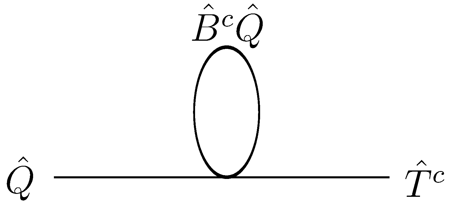
Figure 8: Superfield diagrams for proper self-energy, (a) for $\Sigma^{b}_{+-}(p,\theta^{2})$ and (b) for $\Sigma^{t}_{+-}(p,\theta^{2})$, with the dimension five four-superfield interaction.

 

The basic Lagrangian, in the presence of $\hat{Q}\hat{T^{c}}$ and $\hat{Q}\hat{B^{c}}$ composites as the effective $\hat{H}_{d}$ and $\hat{H}_{u}$, respectively, can be easily extended to give the full MSSM Lagrangian as the effective theory 034 . For the superfield gap equation analysis, we have to consider the two Dirac mass terms

$$\int\!\!d^{4}\theta~{}\left[({\mathcal{M}}_{t}\,\hat{Q}\hat{T^{c}}+{\mathcal{M}}_{b}\,\hat{Q}\hat{B^{c}})\,\delta^{2}\!(\bar{\theta})+h.c.\right]\;,$$ (63)

with

$${\mathcal{M}}_{t}=m_{t}-{\theta}^{2}\eta_{t}\;,$$

$${\mathcal{M}}_{b}=m_{b}-{\theta}^{2}\eta_{b}\;.$$ (64)

We need the propagator $\left\langle T\left(\hat{Q}(1)\hat{T^{c}}(2)\right)\right\rangle$ given explicitly above together with an exact matching one for $\left\langle T\left(\hat{Q}(1)\hat{B^{c}}(2)\right)\right\rangle$ (with all subscript $t$ replaced by $b$). Following the calculations as illustrated in the main text with $\Sigma^{b}_{+-}(p,\theta^{2})$ shown in Fig. 8, we have

$$m_{b} = 2\frac{\bar{\eta}_{t}G}{2}\;I^{\prime}_{2}(|m_{t}|^{2},\tilde{m}_{Q}^{2},\tilde{m}_{t}^{2},|\eta_{t}|,\Lambda^{2})\;,$$

$$\eta_{b} = 2\bar{m}_{t}G\;I^{\prime}_{1}(|m_{t}|^{2},\tilde{m}_{Q}^{2},\tilde{m}_{t}^{2},|\eta_{t}|,\Lambda^{2})-2\frac{\bar{\eta}_{t}GB}{2}\;I^{\prime}_{2}(|m_{t}|^{2},\tilde{m}_{Q}^{2},\tilde{m}_{t}^{2},|\eta_{t}|,\Lambda^{2})\;.$$ (65)

Similarly, $\Sigma^{t}_{+-}(p,\theta^{2})$ shown in Fig. 8 gives

$$m_{t} = 2\frac{\bar{\eta}_{b}G}{2}\;I^{\prime}_{2}(|m_{b}|^{2},\tilde{m}_{Q}^{2},\tilde{m}_{b}^{2},|\eta_{b}|,\Lambda^{2})\;,$$

$$\eta_{t} = 2\bar{m}_{b}G\;I^{\prime}_{1}(|m_{b}|^{2},\tilde{m}_{Q}^{2},\tilde{m}_{b}^{2},|\eta_{b}|,\Lambda^{2})-2\frac{\bar{\eta}_{b}GB}{2}\;I^{\prime}_{2}(|m_{b}|^{2},\tilde{m}_{Q}^{2},\tilde{m}_{b}^{2},|\eta_{b}|,\Lambda^{2})\;,$$ (66)

[where $I^{\prime}_{1}(|m_{t}|^{2},\tilde{m}_{Q}^{2},\tilde{m}_{t}^{2},|\eta_{t}|,\Lambda^{2})$ and $I^{\prime}_{2}(|m_{t}|^{2},\tilde{m}_{Q}^{2},\tilde{m}_{t}^{2},|\eta_{t}|,\Lambda^{2})$ can be obtained from $I^{\prime}_{1}(|m_{b}|^{2},\tilde{m}_{Q}^{2},\tilde{m}_{b}^{2},|\eta_{b}|,\Lambda^{2})$ and $I^{\prime}_{2}(|m_{b}|^{2},\tilde{m}_{Q}^{2},\tilde{m}_{b}^{2},|\eta_{b}|,\Lambda^{2})$ by the replacements $m_{b}$ by $m_{t}$, $\tilde{m}_{b}^{2}$ by $\tilde{m}_{t}^{2}$ and $\eta_{b}$ by $\eta_{t}$]. In both cases there is extra factor 2 which appears from the color factor. (In fact, the interaction term with the color indices reads $\hat{Q}^{\alpha}\hat{T}^{c}_{\alpha}\hat{Q}^{\beta}\hat{B}^{c}_{\beta}$ without which the indistinguishable $\hat{Q}^{\alpha}$ and $\hat{Q}^{\beta}$ giving vanishing result as the singlet direction is antisymmetric in the $SU(2)$ indices of the two $\hat{Q}$ doublets — hence the factor 2 instead of 3.)

We have the model gap equations as given by Eqns.(66) and (65). Nontrivial solutions to the two superfield Dirac mass parameters ${\mathcal{M}}_{t}$ and ${\mathcal{M}}_{b}$ correspond to electroweak symmetry breaking with two $SU(2)\times U(1)$ doublets aligned to preserve the electromagnetic $U(1)$. We have to leave reporting nontrivial solutions for the generic case to a future publication, due to the very demanding analysis involved. However, we can again use a simple, special, case to establish that the usual electroweak symmetry breaking can be obtained. If we take $\tilde{m}_{b}^{2}=\tilde{m}_{t}^{2}$ in the original Lagrangian of Eqn.(62), the model dynamic is obviously symmetrical for $t$ and $b$. That naturally suggests looking for solution with ${\mathcal{M}}_{t}={\mathcal{M}}_{b}$. In this case, the two set of gap equations collapsed into one. Take further the same soft mass value for $\tilde{m}_{Q}^{2}$. The set of gap equations then becomes identical to the one of our prototype model discussed in the main text, with nontrivial solution explicitly illustrated. Under the special case, we have electroweak symmetry breaking for the MSSM, with however phenomenologically wrong identical top and bottom masses. To get the right masses, we sure need $\tilde{m}_{b}^{2}\neq\tilde{m}_{t}^{2}$ as a starting point.

Our key purpose here is to illustrate explicitly the HSNJL model as one that is capable of giving rising to dynamical symmetry breaking and Dirac mass generation, including interesting continuous symmetry like $SU(2)\times U(1)$. The most phenomenologically interesting application would be for the case with the MSSM as the effective field theory, which we also discussed here. The model can also be easily applied to other symmetry breaking setting of possible phenomenological interest, such as a grand unification symmetry.

References

(1)
Y. Nambu, Nobel Lecture: Spontaneous Symmetry Breaking in
Particle Physics: A Case of Cross Fertilization, Int. J. Mod.
Phys. A 24, 2371 (2009), Rev. Mod. Phys.81
1015 (2009).
(2)
Y. Nambu and G. Jona-Lasinio, Dynamical Model of Elementary Particles Based on an Analogy with
Superconductivity. I, Phys. Rev.122 (1961) 345;
Dynamical Model of Elementary Particles Based on an Analogy with
Superconductivity. II,ibid.124 (1961) 246.
(3)
Y. Nambu, Axial Vector Current Conservation in Weak
Interactions, Phys. Rev. Lett.4 (1960) 380.
(4)
Y. Nambu, Enerico Fermi Institute Report No. 89-08 (1989), Bootstrap Symmetry Breaking in Electroweak Unification.
(5)
V. Miransky, M. Tanabashi, and K. Yamawaki, Is the t Quark
Responsible for the Mass of W and Z Bosons?, Mod. Phys. Lett. A
4 (1989) 1043; Dynamical Electroweak Symmetry Breaking
with Large Anomalous Dimension and t Quark Condensate, Phys.
Lett. B 221 (1989) 177; W.J. Marciano, Heavy Top
Quark Mass Predictions, Phys. Rev. Lett.62 (1989) 2793;