Pre-dewetting transition on a hydrophobic wall: Statics and dynamics

Abstract

For one-component fluids, we predict a pre-dewetting phase transition between a thin and thick low-density layer in liquid on a wall repelling the fluid. This is the case of a hydrophobic wall for water. A pre-dewetting line starts from the coexistence curve and ends at a surface critical point in the phase diagram. We calculate this line numerically using the van der Waals model and analytically using the free energy expansion up to the quartic order. We also examine the pre-dewetting dynamics of a layer created on a hydrophobic spot on a heterogeneous wall. It is from a thin to thick layer during decompression and from a thick to thin layer during compression. Upon the transition, a liquid region above the film is cooled for decompression and heated for compression due to latent heat convection and a small pressure pulse is emitted from the film into the liquid.

I Introduction

Extensive efforts have been made on the wetting transitions for various liquids and walls both theoretically and experimentally Cahn ; PG ; Bonnreview . As is well-known, when a liquid droplet is placed on a wall in gas, the three-phase contact angle changes from a finite value (partial wetting) to zero (complete wetting) at a wetting transition temperature $T_{\rm w}$ on the coexistence curve. Furthermore, there is a phase transition of adsorption between a thin and thick liquid layer across a prewetting line outside the coexistence curve Cahn ; Ebner ; Bonnreview ; Evans . For one-component fluids, the line starts from the wetting transition point $T=T_{\rm w}$ on the coexistence curve and ends at a surface critical point at $T=T_{c}^{\rm pw}$ in the $T$-$n$ or $T$-$p$ plane, where $n$ and $p$ are the density and the pressure in the surrounding gas region.

On the other hand, many authors have been interested in the structural change in the hydrogen bonding network formed by the water molecules in the vicinity of a hydrophobic surface Is ; Sti ; Pratt ; Ro ; Berne ; Chandler1999 ; Ash ; Koishi ; Netz ; Chandler . We also mention many observations of surface bubbles or films on mesoscopic scales (with 10-100 nm thickness) on hydrophobic walls in water Higashi ; Zhang ; Attard ; Loshe . Here the attractive interaction among the water molecules arise from the hydrogen bonding. As a result, there can even be a gas region in contact with a hydrophobic surface in liquid water at room temperature and at the atmospheric pressure ($\sim 1$atom). To support this behavior, the solvation free energy $\Delta G_{\rm sol}$ of a hydrophobic particle with radius $R$ in water is nearly given by $4\pi R^{2}\sigma$ per particle for relatively large $R(\gtrsim 1$nm) Chandler , where $\sigma$ is the gas-liquid surface tension.

In this paper, we examine whether or not a low-density film in liquid on a hydrophobic wall undergoes a pre-dewetting phase transion between a thin and thick low-density layer. As in the prewetting case, a pre-dewetting line should start from a point, $T=T_{\rm cx}^{dw}$, on the coexistence curve and ends at a pre-dewetting critical point. It follows complete dewetting for $T>T_{\rm cx}^{dw}$ on the coexistence curve. We develop a mean-field theory based on the Ginzburg-Landau model as in the original paper Cahn . Our calculations are thus performed rather close to the critical point (at $T\sim 0.9T_{c})$, where the film density is not very small compared to the ambient liquid density.

Furthermore, we are interested in the dynamics of the wetting transition of volatile liquids, where understanding of evaporation and condensation at the interface is still inadequate Bonn ; Hardy ; Dussan . For example, Koplik et al. p3 performed molecular dynamic simulation to observe evaporation of a droplet and a decrease of the contact angle upon heating a wall in partial wetting. Gu$\acute{\rm e}$na et al. Caza performed an experiment, where a weakly volatile droplet spread as an involatile droplet in an initial stage but disappeared after a long time due to evaporation in complete wetting. In a near-critical one-component fluid, Hegseth et al. Hegseth observed that a bubble was attracted to a heated wall even when it was completely wetted by liquid in equilibrium. To study such problems, we have recently developed a phase-field model for compressible fluids with inhomogeneous temperature, called the dynamic van der Waals model Onuki . (See a review on various phase-field theories of fluids phase1 .) In our framework, we may describe the gas-liquid transition and convective latent heat transport without assuming any evaporation formula. We then numerically investigated evaporation of a liquid droplet on a heated substrate Teshi1 and spreading of a liquid film on a cooled or warmed substrate for a one-component fluid Teshi2 . The lattice Boltzmann method has been applied to two-phase fluids also Y ; Pooly ; In . However, this method has not yet been fully developed to describe evaporation and condensation.

This paper also presents simulation results on the film dynamics using the numerical method in our previous studies Teshi1 ; Teshi2 . We initially start with an equilibrium thin or thick film on a wall at the bottom near the pre-dewetting transition and then cool or heat the temperature at the top. (We use ”bottom” and ”top” though we do not assume gravity.) Subsequently, the cell is gradually decompressed or compressed and the pre-dewetting transition is induced in the film.

The organization of this paper is as follows. In Sec.II, we will examine the static aspect of the pre-dewetting transition in the Ginzburg-Landau scheme Cahn ; PG in the mean field theory. In Sec.III, we will apply the dynamic van der Waals model to investigate the pre-dewetting dynamics by cooling and heating the top plate of a cylindrical cell. In the appendix, the pre-dewetting transition will be examined near the critical point by expanding the free energy with respect to the density $n$ around the critical density $n_{c}$ up to the quartic order.

II Statics

II.1 Ginzburg-Landau model

We consider a one-component fluid in contact with a sold wall in equilibrium, where the number density $n$ is the order parameter. Assuming short-ranged forces, we set up the free energy $F$ with the gradient contribution as Onukibook ; vander

$${F}=\int d{\mbox{\boldmath$r$}}\bigg{[}{f(n,T)}+\frac{1}{2}M|\nabla n|^{2}\bigg{]}+\int da\gamma n,$$ (2.1)

where the integral is in the fluid container in the first term and on the wall surface in the second term ($\int da$ being the surface integral). As a function of $n$ and $T$, $f=f(n,T)$ is the Helmholtz free energy density. In our numerical calculation, we will use the simple van der Waals form Onukibook ,

$$f=k_{B}Tn\bigg{[}\ln[{n\lambda_{\rm th}^{3}}/({1-v_{0}n})]-1\bigg{]}-\epsilon v_{0}n^{2},$$ (2.2)

where $v_{0}$ is the molecular volume, $\epsilon$ is the magnitude of the attractive pair potential, and $\lambda_{\rm th}=\hbar(2\pi/mk_{B}T)^{1/2}$ is the thermal de Broglie length with $m$ being the molecular mass. The coefficient $M$ of the gradient free energy will be assumed to be independent of $n$ but proportional to $T$. The last term is the surface free energy expressed as the integration on the solid surface Cahn ; PG ; Bonnreview , where the second-order term of the form $M\lambda_{e}^{-1}(n-n_{c})^{2}/2$ (present in the original work Cahn ) is neglected. (This is allowable for very large $|\lambda_{e}|$ compared to the correlation length Binderreview .) In the literature Bonnreview ; Binderreview , the so-called surface field is given by $-\gamma$. For water-like fluids, $\gamma>0$ for a hydrophobic surface and $\gamma<0$ for a hydrophilic surface. For this surface free energy, the pre-dewetting transition occurs for $\gamma>0$, while the prewetting transition for $\gamma<0$.

In equilibrium, the space-dependent density $n=n({\mbox{\boldmath$r$}})$ in the bulk region is determined by

$$\mu-M\nabla^{2}n=\mu_{0}$$ (2.3)

where $\mu=\partial f/\partial n$ is the chemical potential and $\mu_{0}$ is a constant. The left hand side $\mu-M\nabla^{2}n$ represents the generalized chemical potential including the gradient contribution. On the wall surface we have

$$M{\mbox{\boldmath$\nu$}}\cdot\nabla n=\gamma,$$ (2.4)

where $\nu$ is the outward normal unit vector (from the wall to the fluid) on the wall surface.

II.2 Pre-dewetting transition for $n_{0}>n_{c}$

Let us consider an equilibrium one-component fluid in the region $z>0$ in contact with a planar substrate with $\gamma>0$ placed at $z=0$. In this one-dimensional geometry, all the quantities depend only on $z$. The density $n(z)$ tends to a constant liquid density $n_{0}$ far from the wall. The pressure and the chemical potential far from the wall are written as $p_{0}$ and $\mu_{0}$, respectively, where $p_{0}=n_{0}k_{B}T/(1-v_{0}n_{0})-v_{0}\epsilon n_{0}^{2}$ for the van der Waals model (2.2). In equilibrium, we should minimize the grand potential $\Omega$ (per unit area) given by

$$\Omega=\int_{0}^{\infty}dz[\omega+\frac{1}{2}M|n^{\prime}|^{2}]+\gamma n_{s},$$ (2.5)

where $n^{\prime}=dn/dz$ and $n_{s}$ is the surface density,

$$n_{s}=n(0).$$ (2.6)

We introduce the grand potential density as

$$\omega=f-\mu_{0}n+p_{0},$$ (2.7)

Use of the van der Waals form (2.2) gives

$$\omega = k_{B}Tn\ln\bigg{[}\frac{n(1-v_{0}n_{0})}{n_{0}(1-v_{0}n)}\bigg{]}-k_{B}T\frac{n-n_{0}}{1-v_{0}n_{0}}$$ (2.8)

$$-\epsilon v_{0}(n-n_{0})^{2}.$$

Far from the wall, $\omega$ behaves as $\omega\cong\chi(n_{0})(n-n_{0})^{2}/2$ and tends to zero. We define

$$\chi(n)=\partial^{2}f/\partial n^{2}=1/n^{2}K_{T},$$ (2.9)

where $K_{T}$ is the isothermal compressibility.

In the region $z>0$, the density profile $n=n(z)$ is determined by $\mu-Mn^{\prime\prime}=\mu_{0}$ from Eq.(2.3), where $n^{\prime\prime}=d^{2}n/dz^{2}$. We multiply this equation by $n^{\prime}$ and integrate the resultant one with respect to $z$ to obtain Onukibook

$$\omega=M|n^{\prime}|^{2}/2.$$ (2.10)

From Eq.(2.4) the boundary condition at $z=0$ reads

$$Mn^{\prime}(0)=\gamma.$$ (2.11)

On the basis of the van der Waals model (2.2), we introduce a microscopic length $\ell$ defined by

$$\ell=(M/2k_{B}Tv_{0})^{1/2}.$$ (2.12)

Since $\gamma>0$, Eq.(2.10) is rewritten as

$$n^{\prime}(z)=\sqrt{2\omega(n(z))/M}=\ell^{-1}\sqrt{\omega(n(z))/k_{B}Tv_{0}},$$ (2.13)

where $\omega$ is treated as a function of $n$ and its $T$ dependence is suppressed. Using $\ell$, we integrate this equation as

$$z=\ell\int_{n_{s}}^{n}dn/\sqrt{\omega(n)/k_{B}Tv_{0}}.$$ (2.14)

From Eqs.(2.11) and (2.13) we have

$$\gamma=\sqrt{2M\omega(n_{s})}=2\ell\sqrt{k_{B}Tv_{0}\omega(n_{s})}.$$ (2.15)

Using Eq.(2.13) we rewrite Eq.(2.5) as Cahn

$$\Omega=\int_{n_{s}}^{n_{0}}dn[\sqrt{2M\omega(n)}-\gamma]+\gamma n_{0},$$ (2.16)

where the integrand vanishes at the lower bound $n=n_{s}$ from Eq.(2.15).

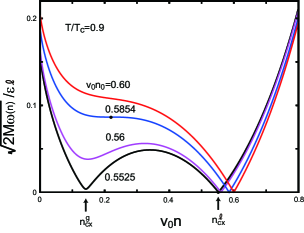
Figure 1: (Color online) $\sqrt{2M\omega(n)}/{\epsilon\ell}$ vs $v_{0}n$ at $T/T_{c}=0.9$ for $v_{0}n_{0}=0.5525$, $0.56,0.58,0.60$ from below, where the smallest one is very close to the coexistence liquid density $n_{\rm cx}^{\ell}=0.5524$. Use is made of the van der Waals form (2.8).

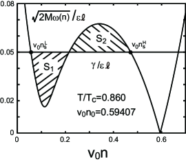
Figure 2: Illustration of a pre-dewetting transition, where $\sqrt{2M\omega(n)}/\epsilon\ell$ is plotted for $T/T_{c}=0.860$ and $v_{0}n_{0}=0.59407$. At $\gamma/\epsilon\ell=0.05$, the areas of the regions $S_{1}$ and $S_{2}$ coincide, leading to the same value of $\Omega$ in Eq.(2.16) at two surface densities $n_{s}=n_{s}^{L}$ and $n_{s}^{H}$.

Cahn Cahn showed that the thickness of a film of the preferred phase on a wall grows logarithmically as the surrounding fluid approaches a state on the coexistence curve. In our case, the film thickness $D$ increases logarithmically as $n_{0}$ approaches the liquid density on the coexistence curve $n_{\rm cx}^{\ell}$, where we may take the isothermal path of approach, for example. To show this, we expand the free energy density $f$ around the corresponding gas density on the coexistence curve $n_{\rm cx}^{g}$ as

$$f\cong-p_{\rm cx}+\mu_{\rm cx}n+\chi_{g}(n-n_{\rm cx}^{g})^{2}/2,$$ (2.17)

where $p_{\rm cx}$ and $\mu_{\rm cx}$ are the pressure and the chemical potential, respectively, on the coexistence curve. When the bulk density $n_{0}$ is slightly larger than $n_{\rm cx}^{\ell}$, we have $(p_{0}-p_{\rm cx})/n_{\rm cx}^{\ell}\cong\mu_{0}-\mu_{\rm cx}\cong\chi_{\ell}(n_{0}-n_{\rm cx}^{\ell})$, so that

$$\omega\cong\chi_{g}(n-n_{\rm cx}^{g})^{2}/2+\chi_{\ell}(n_{\rm cx}^{\ell}-n_{\rm cx}^{g})(n_{0}-n_{\rm cx}^{\ell}).$$ (2.18)

Substitution of this relation into Eq.(2.14) yields

$$D\cong\xi_{g}\ln\bigg{[}\frac{2\chi_{g}(n_{\rm cx}^{g}-n_{s})}{\chi_{\ell}(n_{0}-n_{\rm cx}^{\ell})}\bigg{]},$$ (2.19)

where $\chi_{g}=\chi(n_{\rm cx}^{g})$ and $\chi_{\ell}=\chi(n_{\rm cx}^{\ell})$ are defined on the coexistence curve and $\xi_{g}=(M/\chi_{\rm cx}^{g})^{1/2}$ is the correlation length in the gas phase. As $n_{0}-n_{\rm cx}^{\ell}$ tends to zero, a well-defined interface appears.

In Fig.1, we plot $\sqrt{2M\omega(n)}/\epsilon\ell=2\sqrt{k_{B}Tv_{0}\omega(n)}/\epsilon$ vs $v_{0}n$ at $T=0.9T_{c}$ for four bulk densities $n_{0}$, using the van der Waals model (2.8). (i) The smallest bulk density is $0.5525v_{0}^{-1}$, which is slightly larger than the coexistence liquid density $n_{\rm cx}^{\ell}=0.5524v_{0}^{-1}$. As a result, $\omega(n)$ nearly vanishes at the coexistence gas density $n_{\rm cx}^{g}=0.1419v_{0}^{-1}$. The gas layer thickness $D$ is logarithmically dependent on $n_{0}-n_{\rm cx}^{\ell}$ as in Eq.(2.19). (ii) At $n_{0}=0.56v_{0}^{-1}$, there are a minimum and a maximum satisfying $\partial\omega/\partial n=f^{\prime}-\mu_{0}=0$. (iii) At $n_{0}=0.5854v_{0}^{-1}$, the two extrema merge into a point $n=n_{\rm sc}$, at which $\partial^{2}\omega/\partial n^{2}=\chi=0$ holds and $n_{\rm sc}$ coincides with the so-called spinodal density on the gas branch for the linear form of the surface free energy. (iv) At $n_{0}=0.60v_{0}^{-1}$, $\sqrt{\omega(n)}$ increases with decreasing $n$ in the range $n<n_{0}$. Then Eq.(2.15) yields a unique surface density $n_{s}$ for any $\gamma>0$.

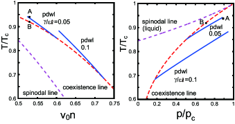
Figure 3: (Color online) Pre-dewetting lines (pdwl) for $\gamma/\epsilon\ell=0.05$ and 0.10 in the $T$-$n$ plane (left) and in the $T$-$p$ plane (right), where $n$ and $p$ are the bulk values (written as $n_{0}$ and $p_{0}$ in the text). Each pdwl starts from a point on the coexistence curve, where $T=T_{\rm cx}^{\rm dw}(\gamma)$ and $p=p_{\rm cx}^{\rm dw}(\gamma)$, and ends at a pre-dewetting critical point, where $T=T_{c}^{\rm dw}(\gamma)$ and $p=p_{c}^{\rm dw}(\gamma)$. See Sec.III for nonequilibrium simulations starting with points A and B as initial equilibrium states.

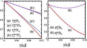
Figure 4: (Color online) Left: (a) Pre-dewetting temperature $T_{\rm cx}^{\rm dw}$ on the coexistence curve and (b) pre-dewetting critical temperature $T_{c}^{\rm dw}$ as functions of $\gamma/\epsilon\ell$. Their linear approximations are (a’) $T_{\rm cx}^{\rm dw,0}$ and (b’) $T_{c}^{\rm dw,0}$ (see Eqs.(2.22) and (2.23)). Right: (a) Pre-dewetting pressure $p_{\rm cx}^{\rm dw}$ on the coexistence curve and (b) pre-dewetting critical pressure $p_{c}^{\rm dw}$ as functions of $\gamma/\epsilon\ell$.

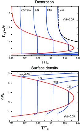
Figure 5: (Color online) Normalized desorption $v_{0}\ell^{-1}\Gamma_{1d}$ in Eq.(2.25) (top) and normalized surface density $v_{0}n_{s}$ (bottom) as functions of $T/T_{c}$ for $v_{0}n_{0}=0.59,0.57,0.55,$ and 0.53 (from left) at $\gamma/\epsilon\ell=0.05$. They change discontinuously across the pre-dewetting transition. Theoretical curve for $v_{0}\ell^{-1}\Gamma_{1d}$ from the Landau expansion is shown for $v_{0}n_{0}=0.53$ (broken line, rightest in top plate).

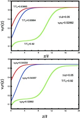
Figure 6: (Color online) Normalized density profile $v_{0}n(z)$ vs normalized distance $z/\ell$ from a wall at $\gamma/\epsilon\ell=0.05$. Shown are those for $T/T_{c}=0.93665,0.93664$, and 0.92 at $v_{0}n_{0}=0.52892$ (top) and those for $v_{0}n_{0}=0.54358,0.54357$, and 0.52892 at $T/T_{c}=0.92$ (bottom). The first two curves from above are taken just before and after the pre-dewetting transition, while the third one close to the coexistence curve.

As illustrated in Fig.2, a pre-dewetting transition appears when the curve of $\sqrt{\omega(n)}$ has two extrema as in the case of $n_{0}=0.56v_{0}^{-1}$ in Fig.1. That is, if the areas $S_{1}$ and $S_{2}$ are equal, a first-order transition occurs between two surface densities $n_{s}^{L}$ and $n_{s}^{H}$. For each given $\gamma>0$, a pre-dewetting line starts from a temperature, $T=T_{\rm cx}^{\rm dw}(\gamma)$, on the coexistence curve and ends at a pre-dewetting critical temperature, $T=T_{c}^{\rm dw}(\gamma)$, outside the coexistence curve. The wall is completely dewetted by the gas phase for $T>T_{\rm cx}^{\rm dw}(\gamma)$ on the coexistence curve.

In Fig.3, two examples of the pre-dewetting line are written for $\gamma/\epsilon\ell=0.05$ and 0.1 in the $T$-$n$ plane (left) and in the $T$-$p$ plane (right), where $n$ and $p$ denote those in the bulk ($n_{0}$ and $p_{0}$). In this paper, the coefficient $M$ is independent of $n$ and is proportional to $T$ as

$$M=TC.$$ (2.20)

Then $C$ and hence $\ell=(C/2v_{0}k_{B})^{1/2}$ are independent of $n$ and $T$. However, essentially the same results were obtained even if $M$ is independent of $T$ (not shown in this paper). We give $T_{\rm cx}^{\rm dw}$ and $T_{c}^{\rm dw}$ and the corresponding densities $n_{\rm cx}^{\rm dw}$ and $n_{c}^{\rm dw}$. For $\gamma/\epsilon\ell=0.05$, we have $(T_{\rm cx}^{\rm dw}/T_{c},v_{0}n_{\rm cx}^{\rm dw})=(0.851,0.601)$ and $(T_{c}^{\rm dw}/Tc,v_{0}n_{c}^{\rm dw})=(0.943,0.524)$. For $\gamma/\epsilon\ell=0.1$, we have $(T_{\rm cx}^{\rm dw}/T_{c},v_{0}n_{\rm cx}^{\rm dw})=(0.683,0.724)$ and $(T_{c}^{\rm dw}/T_{c},v_{0}n_{c}^{\rm dw})=(0.883,0.606)$.

In Fig.4, the left (right) panel displays the pre-dewetting transition temperature (pressure) $T_{\rm cx}^{\rm dw}(\gamma)$ ($p_{\rm cx}^{\rm dw}(\gamma)$) on the coexistence curve and the pre-dewetting critical temperature (pressure) $T_{c}^{\rm dw}(\gamma)$ ($p_{c}^{\rm dw}(\gamma)$) as functions of $\gamma/\epsilon\ell$. For each $\gamma$, the pre-dewetting line is in the range $T_{\rm cx}^{\rm dw}(\gamma)<T<T_{c}^{\rm dw}(\gamma)$. If $\gamma/\epsilon\ell\ll 1$, these temperatures are both close to $T_{c}$ and are expanded with respect to $\gamma$ as

$$T_{\rm cx}^{\rm dw}(\gamma)=T_{c}(1-A_{\rm cx}\gamma/\epsilon\ell+\cdots),$$ (2.21)

$$T_{c}^{\rm dw}(\gamma)=T_{c}(1-A_{c}\gamma/\epsilon\ell+\cdots).$$ (2.22)

On the basis of the van der Waals model (2.2), the coefficients $A_{\rm cx}$ and $A_{c}$ are calculated in the appendix as

$$A_{\rm cx}=\frac{9}{8}\sqrt{2\sqrt{3}+3},\quad A_{c}=\frac{9}{8}.$$ (2.23)

We also plot the linear approximations $T_{\rm cx}^{\rm dw,0}(\gamma)=T_{c}(1-A_{\rm cx}\gamma/\epsilon\ell)$ and $T_{c}^{\rm dw,0}(\gamma)=T_{c}(1-A_{c}\gamma/\epsilon\ell)$, which are indeed in good agreement with the numerical curves for small $\gamma\ll\epsilon\ell$. For the usual prewetting transition in the case $\gamma<0$, the counterparts of $T_{\rm cx}^{\rm dw}$ and $T_{c}^{\rm dw}$ are the wetting temperature $T_{\rm w}$ on the coexistence curve and the prewetting critical temperature $T_{c}^{\rm pw}$. As will be discussed in the appendix, they are expanded as in Eqs. (2.21) and (2.22) if $\gamma$ is replaced by $|\gamma|$.

In Fig.5, we show the desorption $\Gamma_{1d}$ per unit area in the top plate and the surface density $n_{s}$ in the bottom plate as functions of $T/T_{c}$ for $v_{0}n_{0}=0.59,0.57,0.55,$ and 0.53 at $\gamma/\epsilon\ell=0.05$. These lines are outside the coexistence curve in the $T$-$n$ plane. They change discontinuously across the pre-dewetting transition in the range $T_{\rm cx}^{\rm dw}<T<T_{c}^{\rm dw}$. The discontinuities vanish as $T\to T_{c}^{\rm dw}$. We calculate the desorption of the fluid by

$$\Gamma_{1d}=\int_{0}^{\infty}dz[n_{0}-n(r,z)].$$ (2.24)

On each line, as $T\to T_{\rm cx}^{\rm dw}$, $\Gamma_{1d}$ grows logarithmically as $(n_{0}-n_{cx}^{g})D$ with $D$ being given by Eq.(2.20), while $n_{s}$ tends a well-defined limit (see the lower panel of Fig.5). The curve for $v_{0}n_{0}=0.53$ is closest to the pre-dewetting criticality, so we also display its theoretical approximation from the Landau expansion in the appendix.

In Fig.6, we display the density profile $n(z)$ at $\gamma/\epsilon\ell=0.05$. In the top plate we set $T/T_{c}=0.93665,0.93664$, and 0.92 at fixed $n_{0}=0.52892v_{0}^{-1}$, while in the bottom plate we set $v_{0}n_{0}=0.54358,0.54357$, and 0.52892 at fixed $T=0.92T_{c}$. In these plates, the first two curves represent the profiles just before and after the pre-dewetting transition, while the third one is obtained close to the coexistence curve with a well-defined thick gas layer.

II.3 Rough estimates of $C$ and $\gamma$ for water

In our continuum theory, the constant $C$ in Eq.(2.21) and the length $\ell$ in Eq.(2.12) remain arbitrary. For each fluid, we may roughly estimate their sizes with input of the experimental values of $T_{c}$, $n_{c}$, and the surface tension $\sigma$ at some temperature $T$. For example, we have $T_{c}=647$K and $n_{c}=1.076\times 10^{22}$cm^-3 for water. Using these $T_{c}$ and $n_{c}$ in the van der Waals model calculation, we have $\epsilon=28k_{B}T_{c}/8=3.0\times 10^{-17}$mJ and $v_{0}=(3n_{c})^{-1}=31\times 10^{-24}$cm³, from which we define the van der Waals radius by $a_{\rm vdw}=v_{0}^{1/3}=3.1{\rm\AA}$. For water, an experimental surface tension is $\sigma=9.3$mJ$/$m² $=0.030\epsilon/a^{2}$ at $T=0.92T_{c}$ Kislev . On the other hand, from the model (2.1) under Eqs.(2.12) and (2.21), the surface tension is numerically calculated as $\sigma_{\rm vdw}=0.0097\epsilon\ell/v_{0}$ at $T=0.92T_{c}$. If we equate these experimental and numerical values of the surface tension, we obtain $\ell\cong 3.1a_{\rm vdw}$ and $C/2k_{B}\sim 10a_{\rm vdw}^{5}$ Kitamura . In the same manner, for argon, we have $\epsilon=0.70\times 10^{-17}$mJ, $v_{0}=4.11\times 10^{21}$cm³, and $\gamma=9.3$mJ$/$m${}^{2}=0.016\epsilon\ell$ at $T=0.92T_{c}$ Buff , leading to $C/2k_{B}\sim 6.8a_{\rm vdw}^{5}$.

For water, we estimate the surface field $\gamma$ by

$$\gamma\sim\sigma/n_{\rm liq},$$ (2.25)

for a typical hydrophobic surface. Here $n_{\rm liq}$ and $\sigma$ are some appropriate liquid density and surface tension. We use the the above-mentioned surface tension for water and set $n_{\rm liq}\sim n_{c}$ to obtain $\gamma/\epsilon\ell\sim 0.03$. This estimation is based on the behavior of the solvation free energy $\Delta G_{\rm sol}$ of a large hydrophobic particle in water Chandler , as discussed in Sec.1.

II.4 Nanobubbles on a hydrophobic spot

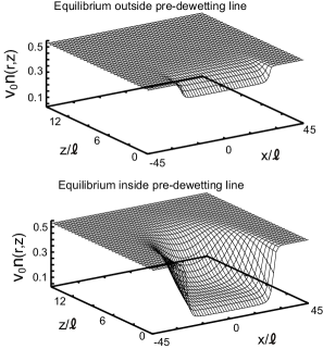
Figure 7: Equilibrium axisymmetric density profile $n(z,r)$ at $y=0$ on a hydrophobic spot with radius $25\ell$, within which $\gamma/\epsilon\ell=0.05$ and outside which $\gamma=0$. Top: $T=0.94T_{c}$, $p_{0}=0.89p_{c}$, and $n_{0}=0.52894v_{0}^{-1}$ at point A in Fig.3, where the fluid is outside the prewetting line and the minimum surface density is $n_{s}=0.40587v_{0}^{-1}$ on the center of the spot. Bottom: $T=0.92T_{c}$, $p_{0}=0.71177p_{c}$, and $n_{0}=0.52925v_{0}^{-1}$ at point B in Fig.3, where the fluid is inside the prewetting line and the minimum surface density is $n_{s}=0.088433v_{0}^{-1}$.

Dewetting as well as wetting is very sensitive to heterogeneity of the substrate. Here we realize bubbles in equilibrium on a heterogeneous surface with a position-dependent $\gamma$.

In this paper, we suppose a circular hydrophobic spot with radius $25\ell$ on the bottom surface by setting

$$\gamma(r) = 0.05\epsilon\ell\quad(r<25\ell),$$ (2.26)

$$= 0~{}~{}~{}\qquad(r>25\ell),$$

where $r=(x^{2}+y^{2})^{1/2}$ at $z=0$. The resultant equilibrium density $n(r,z)$ satisfies Eq.(2.3). Its boundary condition at $z=0$ is given by $\partial n/\partial z=0.05\gamma/M=0.025\epsilon/k_{B}Tv_{0}\ell$ for $r<25\ell$ and $\partial n/\partial z=0$ for $r>25\ell$.

Slightly above the pre-dewetting line, the top plate of Fig.7 gives the cross-sectional density profile $n(r,z)$ at $y=0$ for the point A in Fig.3, where $T=0.94T_{c}$, $p_{0}=0.89p_{c}$, and $n_{0}=0.52894v_{0}^{-1}$. The minimum density is $n_{s}=0.40587v_{0}^{-1}$ at the spot center on the surface. Below the pre-dewetting line, the bottom plate of Fig.7 gives the profile at the point B in Fig.3, where $T=0.92T_{c}$, $p_{0}=0.71177p_{c}$, and $n_{0}=0.52925v_{0}^{-1}$. The minimum density is $n_{s}=0.088433v_{0}^{-1}$ at the spot center. These profiles are very different. To characterize the film size, we introduce the desorption of the fluid by

$$\Gamma=2\pi\int_{0}^{z_{0}}dz\int_{0}^{r_{0}}drr[n_{0}-n(r,z)],$$ (2.27)

where the gas film is well within the integration region $0<z<z_{0}$ and $r<r_{0}$. By setting $z_{0}=15\ell$ and $r_{0}=37.5\ell$, we obtain $\Gamma=339\ell^{3}v_{0}^{-1}$ and $3460\ell^{3}v_{0}^{-1}$ for the top and bottom plates in Fig.7, respectively.

III Dynamics

In this section, using the dynamic van der Waals modelOnuki , we numerically investigate the dynamics of a thin gas layer created on the hydrophobic spot in Eq.(2.27). We treat a one-component fluid without gravity in a temperature range $0.92\leq T/T_{c}\leq 0.94$, where the gas density is $25-30\%$ of the liquid density (see the bottom curves in Fig.6). Then the mean free path in the gas $\ell_{\rm mf}$ is not very long. For very long $\ell_{\rm mf}$, however, numerical analysis based on a continuum phase-field model becomes very difficult. In our simulation, furthermore, relatively small temperature changes are applied and heat and mass fluxes passing through the interface remain weak. As a result, $T$ and the generalized chemical potential (the left hand side of Eq.(2.4)) are continuous across the interface.

In our diffuse interface method, the interface thickness needs to be longer than the simulation mesh size $\Delta x$, so our system size cannot be very large. In our simulation to follow, its length is $150\ell$. Nevertheless, our cell contains many particles about $Vn_{0}\sim 6\times 10^{6}\ell^{3}/v_{0}$, where $V$ is the volume and $n_{0}$ is the initial liquid density.

III.1 Hydrodynamic equations with gradient stress

We set up the hydrodynamic equations for the mass density $\rho=mn$, the momentum density $\rho{\mbox{\boldmath$v$}}$, and the entropy density $\hat{S}$ Teshi1 ; Teshi2 , where $m$ is the molecular mass and $v$ is the velocity field. Here $\hat{S}$ consists of the usual entropy density $ns$ and the negative gradient entropy as

$$\hat{S}=ns-\frac{1}{2}C|\nabla n|^{2}.$$ (3.1)

where $s$ is the entropy per particle and the coefficient $C$ in Eq.(2.21) appears here. The internal energy density, written as $e$, can also contain the gradient contribution, but we neglect it for simplicity Onuki . Then the total Helmholtz free energy density is given by $e-T{\hat{S}}=f+M|\nabla n|^{2}/2$ as in the first term as given in Eq.(2.1). In our scheme, we use the entropy equation instead of the energy equation to achieve the numerical stability in the interface region. That is, with our entropy method, we may remove the so-called parasitic flow at the interface, which has been encountered by many authors para .

We integrated the following hydrodynamic equations without gravity for $\rho$, $\rho{\mbox{\boldmath$v$}}$, and $\hat{S}$ Teshi1 ; Teshi2 :

$$\frac{\partial}{\partial t}\rho+\nabla\cdot(\rho{\mbox{\boldmath$v$}})=0,$$ (3.2)

$$\frac{\partial}{\partial t}\rho{\mbox{\boldmath$v$}}+\nabla\cdot(\rho{\mbox{\boldmath$v$}}{\mbox{\boldmath$v$}}+\tensor{\Pi})=\nabla\cdot\tensor{\sigma},$$ (3.3)

$$\frac{\partial}{\partial t}\hat{S}+\nabla\cdot\bigg{[}\hat{S}{\mbox{\boldmath$v$}}-Cn(\nabla\cdot{\mbox{\boldmath$v$}})\nabla n\bigg{]}=\nabla\cdot\frac{\lambda}{T}\nabla T$$

$$\hskip 56.9055pt+({\dot{\epsilon}_{v}+\dot{\epsilon}_{\theta}})/{T},$$ (3.4)

where the terms in the right hand sides are dissipative. In Eq.(3.3), $\tensor{\Pi}=\{\Pi_{ij}\}$ is the reversible stress tensor,

$$\Pi_{ij} = \bigg{[}p-CT(n\nabla^{2}n+\frac{1}{2}|\nabla n|^{2})\bigg{]}\delta_{ij}$$ (3.5)

$$+CT(\nabla_{i}n)(\nabla_{j}n),$$

where ${p}$ is the van der Waals pressure. Hereafter $\nabla_{i}=\partial/\partial x_{i}$ with $x_{i}$ representing $x$, $y$, or $z$. The terms proportional to $C$ arise from the gradient entropy, constituting the gradient stress tensor. The $\tensor{\sigma}=\{{\sigma}_{ij}\}$ in the right hand side of Eq.(3.3) is the viscous stress tensor,

$${\sigma}_{ij}=\eta(\nabla_{i}v_{j}+\nabla_{j}v_{i})+(\zeta-2\eta/3)(\nabla\cdot{\mbox{\boldmath$v$}})\delta_{ij},$$ (3.6)

in terms of the shear viscosity $\eta$ and the bulk viscosity $\zeta$. In Eq.(3.4), $\lambda$ is the thermal conductivity, while

$$\dot{\epsilon}_{v}=\sum_{ij}\sigma_{ij}\nabla_{j}v_{i},\quad\dot{\epsilon_{\theta}}=\lambda(\nabla T)^{2}/T,$$ (3.7)

are the nonnegative entropy production rates arising from the viscosities and the thermal conductivity, respectively. On approaching equilibrium, $\dot{\epsilon}_{v}$ and $\dot{\epsilon_{\theta}}$ tend to zero, leading to vanishing of the gradients of $v$ and $T$.

The (total) energy density in the bulk is defined by

$$e_{\rm T}={e}+\rho{\mbox{\boldmath$v$}}^{2}/2,$$ (3.8)

which includes the kinetic energy density. The energy-conservation equation reads Landau

$$\frac{\partial}{\partial t}{e}_{\rm T}=-\nabla\cdot\bigg{[}e_{\rm T}{\mbox{\boldmath$v$}}+(\tensor{\Pi}-\tensor{\sigma})\cdot{\mbox{\boldmath$v$}}-\lambda\nabla T\bigg{]}.$$ (3.9)

If Eqs.(3.2) and (3.3) are assumed, the entropy equation (3.4) and the energy equation (3.9) are obviously equivalent. In the text book Landau , however, the entropy equation is derived from the three fundamental conservation equations (3.2), (3.3), and (3.9) Now the total fluid entropy ${\cal S}_{\rm tot}$ and the total fluid energy ${\cal E}_{\rm tot}$ are written as

$${\cal S}_{\rm tot}=\int d{\mbox{\boldmath$r$}}\hat{S},\quad{\cal E}_{\rm tot}=\int d{\mbox{\boldmath$r$}}e_{\rm T}+\int da\gamma n.$$ (3.10)

If the surface field $\gamma$ is independent of $T$ as in Eq.(2.26), the surface term in Eq.(2.1) is the surface energy and there is no surface entropy on all the boundaries. In a fixed cell, we assume the no-slip condition ${\mbox{\boldmath$v$}}={\mbox{\boldmath$0$}}$ on its boundaries. Then the space integrations of Eq.(3.4) and (3.9) yield the time derivatives of ${\cal S}_{\rm tot}$ and ${\cal E}_{\rm tot}$:

$$\frac{d}{dt}{\cal S}_{\rm tot}=\int d{\mbox{\boldmath$r$}}\frac{\dot{\epsilon}_{v}+\dot{\epsilon}_{\theta}}{T}+\int da\frac{{\mbox{\boldmath$\nu$}}\cdot\lambda\nabla T+\gamma\dot{n}}{T},$$ (3.11)

$$\frac{d}{dt}{\cal E}_{\rm tot}=\int da({{\mbox{\boldmath$\nu$}}\cdot\lambda\nabla T+\gamma\dot{n}}),$$ (3.12)

where $\dot{n}=\partial n/\partial t$ and $\gamma$ can be heterogeneous as in Eq.(2.26). If there is no heat input and ${\dot{n}}=0$ on the boundary walls, ${\cal S}_{\rm tot}$ continue to increase monotonically until an equilibrium state is realized.

III.2 Simulation method

We suppose a cylindrical cell in the axisymmetric geometry, where our model fluid is in the region $0\leq z\leq H$ and $0\leq r=({x^{2}+y^{2}})^{1/2}\leq L$. Assuming that all the variables depend only on $z,$ $r$ and $t$, we perform simulations on a two-dimensional $300\times 300$ lattice. We take the simulation mesh length $\Delta x$ equal to $\Delta x=\ell/2$, where $\ell$ is defined in Eq.(2.12). Thus our cell is characterized by

$$H=150\ell,\quad L=150\ell,$$ (3.13)

The velocity $v$ vanishes on all the boundaries. The viscosities and the thermal conductivities are proportional to $n$ as

$$\eta=\zeta=\nu_{0}mn,\quad\lambda=4k_{B}\nu_{0}n.$$ (3.14)

These coefficients are larger in liquid than in gas by the density ratio $n_{\ell}/n_{g}(\sim 5$ in our simulation). The kinematic viscosity $\nu_{0}=\eta/mn$ is a constant. We will measure time in units of the viscous relaxation time,

$$\tau_{0}=\ell^{2}/\nu_{0}=C/2k_{B}v_{0}\nu_{0},$$ (3.15)

on the scale of $\ell$. The thermal diffusion constant $D_{\rm th}=\lambda/C_{p}$ is of order $\nu_{0}$, where $C_{p}$ is the isobaric specific heat per unit volume of order $k_{B}n$ (not very close to the critical point). The time mesh size $\Delta t$ in integrating Eqs.(3.2)-(3.4) is $0.02\tau_{0}$. If the dynamic equations are made dimensionless, there appears a dimensionless number given by $\hat{\sigma}\equiv m\nu_{0}^{2}/\epsilon\ell^{2}$ (written as $\sigma$ in Ref.Onuki ), where $m$ is the molecular mass. The transport coefficients are proportional to $\nu_{0}\propto\hat{\sigma}^{1/2}$. In this paper we set $\sigma=0.06$, for which sound waves are well-defined as oscillatory modes for wavelengths longer than $\ell$ Onuki .

As the boundary conditions, we assume Eq.(2.4) for the density $n$ (even in nonequilibrium) so that $C\partial n/\partial z=0.05\epsilon\ell/T$ on the hydrophobic spot at $z=0$ and ${\mbox{\boldmath$\nu$}}\cdot\nabla n=0$ on all the other surface regions. For the velocity $v$, the no-slip condition ${\mbox{\boldmath$v$}}={\mbox{\boldmath$0$}}$ is assumed. The temperature is fixed at $T_{0}$ at the bottom $z=0$ and at $T_{H}$ at the top $z=H$. The side wall is thermally insulating as $\partial T/\partial r=0$ at $r=L$.

III.3 Decompression by cooling the upper plate

We prepared the equilibrium state at $T=0.94T_{c}$ in the upper plate of Fig.7 as an initial state at $t=0$. We then cooled the top temperature $T_{H}$ from $0.94T_{c}$ to $0.92T_{c}$ fixing the bottom temperature $T_{0}$ at $0.94T_{c}$ for $t>0$. After a very long time $(t>H^{2}/4D_{\rm th}$), the fluid tended to a steady heat-conducting state.

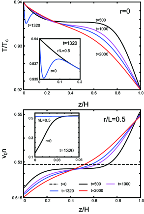
Figure 8: (Color online) Normalized temperature $T(r,z,t)/T_{c}$ at $r=0$ (top) and density $v_{0}n(r,z,t)$ at $r/L=0.5$ (bottom) vs $z/H$ after cooling the top from $0.94T_{c}$ to $0.92T_{c}$. At $t=500\tau_{0}$, thermal diffusion layers appear near the top and bottom, causing an adiabatic change in the middle region. For $t\gtrsim 1000\tau_{0}$, the thermal diffusion extends throughout the cell. The density is decreased in the lower part of the cell, resulting in a homogeneous pressure decrease. Around $t=1320\tau_{0}$, a cool spot appears above the film during the pre-dewetting transition from a thin to thick film. In the inset, the profiles of $T$ and $n$ at $r=0$ and $L/2$ near the bottom are compared.

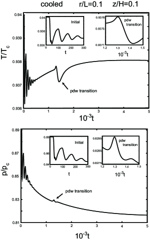
Figure 9: Normalized temperature $T(r,z,t)/T_{c}$ (top) and pressure $p(r,z,t)/p_{c}$ (bottom) as functions of $t$ in units of $\tau_{0}$ in Eq.(3.15) at $(z/H,r/L)=(0.1,0.1)$ (slightly above the gas film) after cooling the top. Two insets in each panel show initial oscillatory behavior due to sound wave propagation (left) and a sudden change at the prewetting transition (right).

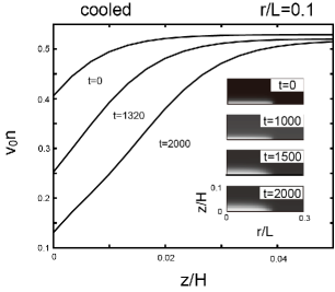
Figure 10: Normalized density $v_{0}n(r,z,t)$ vs $z/H$ at $r/H=0.1$ for $t/\tau_{0}=0$, $1320$, and $2000$ from above after cooling the top. At $t=1320\tau_{0}$, the film thickness is increasing abruptly at the pre-dewetting transition, while at $t=2000\tau_{0}$ it is still increasing slowly (see Fig.11). Cross-sectional film profiles are also given in the right, where the darkness represents the density at four times.

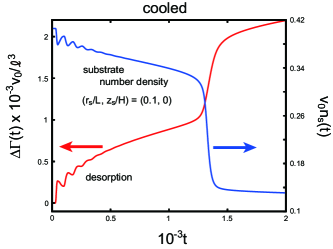
Figure 11: Normalized excess desorption $v_{0}\ell^{-3}\Delta\Gamma(t)$ in Eq.(3.16) and surface density $v_{0}n_{s}(r,t)$ vs $t$ at $r/L=0.1$ in units of $\tau_{0}$ after cooling the top. They exhibit oscillatory behavior in the initial stage and an abrupt change at the pre-dewetting transition taking place in a time interval of $250\tau_{0}$.

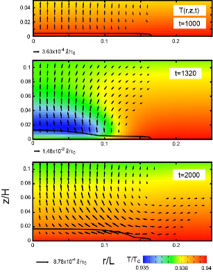
Figure 12: (Color online) Temperature $T(r,z,t)$ in gradation at $t/\tau_{0}=1000,1320$, and $2000$ around the hydrophobic spot. On the block line, $|\nabla n|$ is largest, indicating the film location. Arrows indicate the velocity $v$. Their amplitudes are known from reference arrows below the middle abd bottom panels. The liquid region above the film is cooled due to latent heat absorption to the film at the pre-dewetting transition. The profile at $t=2000\tau_{0}$ (bottom) is nearly stationary, where condensation is taking from the side and evaporation from the upper surface. The colors represent $T/T_{c}$ according to the color bar at the bottom.

In Fig.8, we show the profiles of the temperature $T(r,z,t)$ at $r=0$ and the density $n(r,z,t)$ at $r=L/2$ as functions of $z$ to illustrate how cooling and decompression are realized in the cell. In the initial stage, the piston effect is operative, which has been studied theoretically Ferrell ; Zappoli and experimentally Beysens ; Moldover ; Miura . In this situation, there appear a compressed thermal diffusion layer at the top and an expanded one at the bottom with thickness growing in time as $\ell_{\rm D}(t)=(D_{\rm th}t)^{1/2}$, which produce sound waves propagating in the cell and causes an adiabatic change outside the diffusion layers. The sound velocity in the present case is about $c=4\ell/\tau_{0}$, so the acoustic traversal time over the cell is $H/c\sim 35\tau_{0}$. In fact, at $t=500\tau_{0}$, $T$ and $n$ are flat in the middle region, where $T$ and $n$ are changed adiabatically. However, in the late stage $t\gtrsim 1000\tau_{0}$, the layer thickness reaches $H/2$ and the thermal diffusion becomes relevant throughout the cell. In all these processes, the pressure $p$ is kept nearly homogeneous in the cell.

In our problem, we should focus on the behavior of $T$ and $p$ around the gas film on the hydrophobic spot. The film is under gradual decompression, but nearly at the initial temperature (since the bottom temperature is pinned). As a result, at $t=1320\tau_{0}$, the pre-dewetting transition takes place from a thin to thick gas film. This is indicated by formation of a cool spot in the liquid above the film in Fig.8. It is caused by the latent heat adsorption to the expanding film at the first-order phase transition (see Fig.12 in more detail). There is no cooling outside the film region $r/L\gtrsim 0.2$.

In Fig.9, we display the temperature $T(r,z,t)$ and the pressure $p(r,z,t)$ slightly above the film at a fixed position located at $(z/H,r/L)=(0.1,0.1)$. In the early stage $t\lesssim 300\tau_{0}$, we can see their oscillatory relaxations caused by sound wave traversals. Upon occurrence of the pre-dewetting transition at $t\sim 1300\tau_{0}$, we can see a small drop in $T$ of order $5\times 10^{-4}T_{c}$ and a small peak in $p$ of order $10^{-3}p_{c}$ on their curves. However, the insets in Fig.9 reveal that their behavior is somewhat complicated on a short time scale of order $50\tau_{0}$, because they change on arrivals of a sound wave and a velocity disturbance from the film. At long times, $T$ tends to a constant about $0.938T_{c}$, but $p$ continues to decrease slowly.

In Fig.10, the profiles of the density $n(r,z,t)$ vs $z$ are given at $r/H=0.1$ at three times together with their cross-sectional profiles. The increase in the film thickness is abrupt around $t=1320\tau_{0}$ at the pre-dewetting transition and is very slow at $t=2000\tau_{0}$. Figure 11 presents the time evolution of the surface density $n_{s}(r,t)$ at $r/L=0.1$ and the excess desorption $\Delta\Gamma(t)$ defined by

$$\Delta\Gamma(t)=2\pi\int_{0}^{z_{0}}dz\int_{0}^{r_{0}}drr[(n_{0}(r,z)-n(t,r,z))],$$ (3.16)

where $n_{0}(r,z)=n(0,r,z)$ is the initial density profile and we set $z_{0}=0.1H$ and $r_{0}=0.25L$. The initial oscillatory relaxations arise from traversals of sound waves, while $n_{s}$ decreases and $\Gamma$ increases abruptly at the pre-dewetting transition at $t\sim 1.3\times 10^{3}\tau_{0}$. We recognize that the pre-dewetting transition from a thin to thick film occurs in a time of order $250\tau_{0}$.

In Fig.12, we show $T(r,z,t)$ in gradation at $t/\tau_{0}=1000,1320$, and $2000$ around the hydrophobic spot. Since there is no clear interface here, a gas-liquid boundary is indicated by a line on which $|\nabla n|$ is largest in the direction of $\nabla n$. We also display the velocity $v$ by arrows. The reference arrow below each panel represents the maximum velocity, being equal to 0.0363, 1.48, and 0.0878, at $t/\tau_{0}=1000,1320$, and $2000$, respectively, in units of $10^{-2}\ell/\tau_{0}$. It is enhanced in the middle plate at $t/\tau_{0}=1320$ during the pre-dewetting transition, where we can see an upward flow with a magnitude of $1.5\times 10^{-2}\ell/\tau_{0}$ in the liquid region above the expanding film. The expanding velocity of the film is of the same order. If we multiply this velocity by the duration time $250\tau_{0}$ of the transition (which is inferred from Fig.11), we obtain a film thickness of order $D\sim 4\ell$ in accord with the density profiles in Fig.10. The corresponding Reynolds number around the film is about $D|{\mbox{\boldmath$v$}}|/\nu_{0}\sim 0.1$. Remarkably, the region above the film is cooled due to latent heat absorption to the film by $2\times 10^{-3}T_{c}$. The profile at $t=200\tau_{0}$ is nearly stationary, where the typical velocity is of order $5\times 10^{-4}\ell/\tau_{0}$. A balance is attained between condensation from the side and evaporation from the upper surface, while the fluid is at rest far from the film in the presence of a constant temperature gardient. Finally, we give the heat flux $Q_{b}(r,t)=-\lambda\partial T/\partial z$ at $z=0$ from the wall to the fluid at $r=0$ and $L/2$: $(Q_{b}(0,t),Q_{b}(L/2,t)=(1.39,1.13)$ at $t=1000$, $(5.71,0.942)$ at $t=1320$, and $(0.618,0.867)$ at $t=2000$ in units of $10^{-4}\epsilon\ell/v_{0}\tau_{0}$. The heat flux is much enhanced at the center during the pre-dewetting transition. In the inset of the upper panel of Fig.8, the gradient $|\partial T/\partial z|$ is very large at $r=0$, but it is much smaller at $r=L/2$.

III.4 Compression by heating the upper plate

We prepared the equilibrium state at $T=0.92T_{c}$ in the lower plate of Fig.7 (at the point (B) in Fig.3) as an initial state at $t=0$. We then heated the top temperature $T_{H}$ from $0.92T_{c}$ to $0.94T_{c}$ with the bottom temperature $T_{0}$ held fixed at $0.92T_{c}$ for $t>0$.

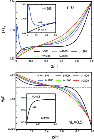
Figure 13: (Color online) $T(r,z,t)/T_{c}$ at $r=0$ (top) and $v_{0}n(r,z,t)$ at $r/L=0.5$ (bottom) vs $z/H$ after heating the top from $0.92T_{c}$ to $0.94T_{c}$. At $t=500\tau_{0}$, thermal diffusion layers appear near the top and bottom. For $t\gtrsim 1000\tau_{0}$, the thermal diffusion extends throughout the cell. The density is increased in the lower part of the cell, resulting in a homogeneous pressure increase. Around $t=1280\tau_{0}$, a heat spot appears above the film during the pre-dewetting transition. In the inset, the profiles of $T$ and $n$ at $r=0$ and $L/2$ near the bottom are compared.

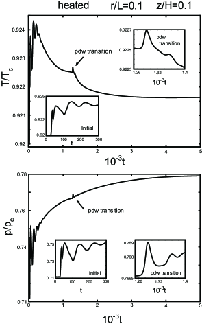
Figure 14: $T(r,z,t)/T_{c}$ (top) and $p(r,z,t)/p_{c}$ (bottom) as functions of $t$ in units of $\tau_{0}$ at $(z/H,r/L)=(0.1,0.1)$ (slightly above the film), after heating the top. Two insets in each panel show initial oscillatory behavior due to sound waves (left) and a sudden change at the pre-dewetting transition from a thick to thin film (right).

In Fig.13, the time evolution of $T(r,z,t)$ at $r=0$ and $n(r,z,t)$ at $r=L/2$ is illustrated as functions of $z$. As in Fig.8, the piston effect takes place in the initial stage, but in the reverse direction. That is, at $t=500\tau_{0}$, there appear an expanded thermal diffusion layer at the top and a compressed one at the bottom. In the late stage $t\gtrsim 1000\tau_{0}$, the thermal diffusion extends over the cell. The pressure $p$ is nearly homogeneous in the cell and increases slowly in time above the initial value. Thus the film is under gradual compression, but nearly at the initial temperature. Occurrence of the pre-dewetting transition is indicated by formation of a heat spot in the liquid above the film at $t=1280\tau_{0}$. It is caused by the latent heat release from the shrinking film (see Fig.17).

Figure 14 displays the temperature $T(r,z,t)$ and the pressure $p(r,z,t)$ at $(z/H,r/L)=(0.1,0.1)$ as in Fig.9. The adiabatic process takes place in the early stage. We find occurrence of the pre-dewetting transition at $t\sim 1280\tau_{0}$, where $T$ and $p$ exhibit a small peak of order $2\times 10^{-4}T_{c}$ and $2\times 10^{-3}p_{c}$, respectively, with a duration time about $50\tau_{0}$. Their detailed behavior can be seen in the insets of Fig.14. At long times, $T$ tends to $0.9216T_{c}$, but $p$ continues to increase slowly.

In Fig.15, the profiles of $n(r,z,t)$ vs $z$ are given at $r/H=0.1$ at three times together with their cross-sectional profiles. The film thickness decreases gradually around $t=1000\tau_{0}$ and is stationary at $t=2000\tau_{0}$. Figure 16 gives the time evolution of the surface density $n_{s}(r,t)$ at $r/L=0.1$ and the excess desorption $\Delta\Gamma(t)$ defined in Eq.(3.16). Here, $n_{s}(r,t)$ increases abruptly around $t=1000\tau_{0}$ as in Fig.11. However, the decrease in $\Delta\Gamma(t)$ is steep in the early stage $t\lesssim 200\tau_{0}$ and is gradual later until $t\sim 1.3\times 10^{3}\tau_{0}$. Evaporation from a thick film is significant in the early stage before the transition.

In Fig.17, we show $T(r,z,t)$ in gradation at $t/\tau_{0}=500,1280$, and $1500$ around the film. The film location is indicated by a line on which $|\nabla n|$ is largest along $\nabla n$. The velocity $v$ is displayed by arrows. We can see a downward flow from the liquid region to the film induced by the film shrinkage. The reference arrow below each panel represents the maximum velocity, being equal to 0.284, 3.54, and 0.0215 at $t/\tau_{0}=500,1280$, and $1500$, respectively, in units of $10^{-2}\ell/\tau_{0}$. The shrinking velocity of the film is of the same order. In contrast to the cooling case in Fig.12, the region above the film is somewhat heated even in the early stage (at $t/\tau_{0}=500$), which is because of the film shrinkage in Fig.11. The heating is most enhanced at $t/\tau_{0}=1280$ in the middle plate during the pre-dewetting transition. The profile at $t=1500\tau_{0}$ is nearly stationary, where a balance is attained between evaporation from the side and condensation from the upper surface. Finally, we give the heat flux $Q_{b}(r,t)=-\lambda\partial T/\partial z$ at $z=0$ from the wall to the fluid at $r=0$ and $L/2$. That is, $(-Q_{b}(0,t),-Q_{b}(L/2,t)=(1.24,1.22)$ at $t=500$, $(44.2,0.870)$ at $t=1280$, and $(1.02,0.871)$ at $t=1500$ in units of $10^{-4}\epsilon\ell/v_{0}\tau_{0}$. The heat flux is much enhanced at the center during the pre-dewetting transition. In the inset of the upper panel of Fig.13, we can see that $\partial T/\partial z$ is large at $r=0$ and is much smaller at $r=L/2$.

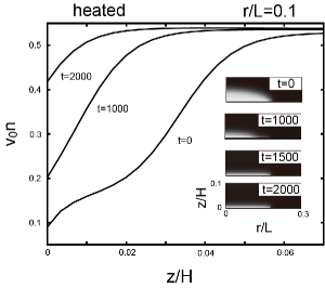
Figure 15: $v_{0}n(r,z,t)$ vs $z/H$ at $r/L=0.1$ for $t/\tau_{0}=0$, $1000$, and $2000$ from below after heating the top. The film thickness decreases as in Fig.16. It is stationary at $t=2000\tau_{0}$. Cross-sectional film profiles are also given in the right, where the darkness represents the density at four times.

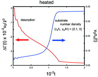
Figure 16: (Color online) Normalized excess desorption $v_{0}\ell^{-3}\Delta\Gamma(t)$ in Eq.(3.16) and surface density $v_{0}n_{s}(r,t)$ vs $t$ at $r/L=0.1$ in units of $\tau_{0}$ after heating the top. Here $n_{s}$ changes abruptly during the pre-dewetting transition in the time region $800\tau_{0}\lesssim t\lesssim 1300\tau_{0}$, but $\Delta\Gamma(t)$ decreases steeply in the initial stage $t\lesssim 200\tau_{0}$. The system becomes stationary for $t\gtrsim 1300\tau_{0}$.

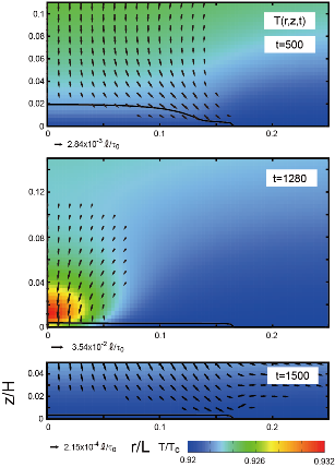
Figure 17: (Color online) Temperature $T(r,z,t)$ at $t/\tau_{0}=500,1280$, and $1500$ around the hydrophobic spot. On the block line, $|\nabla n|$ is largest. Arrows indicate the velocity $v$. Their amplitudes are known from reference arrows below the panels. Even the early stage, the film thickness decreases and the region above the film is heated due to latent heat release. The profile at $t=1500\tau_{0}$ is nearly stationary.

IV Summary and remarks

We summarize our main results.
(i) In Sec.II, for one-component fluids, we have examined the pre-dewetting transition on a hydrophobic wall in the mean-field theory. We have assumed the Ginzburg-Landau free energy for the number density $n$ in the bulk and the surface free energy linear in $n$ with $\gamma$ representing the interaction between the wall and the fluid. Depending on the sign of $\gamma$, a line of prewetting or pre-dewetting appears in the gas or liquid side of the coexistence curve. If $\gamma$ is small, the line is close to the critical point as in Eqs.(2.21) and (2.22). In numerical analysis in Figs. 3,5, and 6, we have set $\gamma=0.05\epsilon\ell$ (where $\epsilon$ is defined in eq.(2.2) and $\ell$ in Eq.(2.12)). For water a rough estimation yields such an order of magnitude of $\gamma$. For real systems it is desirable to measure $\gamma$. In Subsec.IID, we have numerically realized a localized film on a hydrophobic spot in Eq.(2.26), where a thin film is above a pre-dewetting line at $T=0.94T_{c}$ and a thick one is below it at $T=0.92T_{c}$.
(ii) In Sec.III, we have investigated the time evolution of a localized film on the hydrophobic spot in the axisymmetric geometry. Starting with the equilibrium films in Fig.7, we have numerically integrated Eqs.(3.2)-(3.4) after a change of the top temperature from $0.94T_{c}$ to $0.92T_{c}$ in Subsec.IIIC and from $0.92T_{c}$ to $0.94T_{c}$ in Subsec.IIID. Cooling at the top leads to a pressure decrease, while heating at the top leads to a pressure increase. We have found singular behavior at the pre-dewetting transition in the hydrodynamic variables and the excess desorption $\Delta\Gamma(t)$ in Eq.(3.16). Most markedly, the liquid above the film is cooled for decompression and is heated for compression due to latent heat convective transport from the growing or shrinking film, as shown in Figs.8, 12, 13, and 17. A small pressure pulse is emitted from the film to propagate through the cell, as shown in Figs.9 and 14. This pulse could be detected experimentally Miura .

We give some remarks.
(1) A pre-dewetting line as well as a prewetting line readily follows near the critical point for a small surface field $\gamma$. It is then of great interest where we can find a pre-dewetting line for water on a given hydrophobic wall in the phase diagram.
(2) In future work, we should examine the role of the long-ranged van der Waals interaction PG ; Bonnreview ; Ebner ; Evans on the pre-dewetting phase transition.
(3) For water-like polar fluids, a small amount of impurities can strongly promote phase separation due to the solvation effect Current , though we have treated one-component fluids only. As a solute, we may add a noncondensable gas (such as CO₂), hydrophobic particles, or ions in water. Such impurities can strongly affect the formation of surface bubbles or films on a hydrophobic wall in water Higashi ; Zhang ; Attard ; Loshe . We will report shortly on how the pre-dewetting line is shifted downward with increasing the gas concentration.
(4) If the mesh length $\Delta x=\ell/2$ is a few $\rm\AA$, our system length is on the order of several ten manometers and the particle number treated is of order $10^{7}-10^{8}$ (see the beginning of Sec.III). Our continuum description should be imprecise on the angstrom scale. Thus examination of our results by very large-scale molecular dynamics simulations should be informative. We should also investigate how our numerical results can be used or modified for much larger film sizes.
(5) Phase changes inevitably induce a velocity field carrying heat and mass. It has been crucial during the pre-dewetting transition. We have found a steady flow around the film at long times in Figs.12 and 17. In our previous simulation Teshi2 , a steady circular liquid film was realized on a homogeneous wall in the complete wetting condition under a critical heating rate, where evaporation and condensation balanced. It evaporated to vanish for stronger heating, while it expanded for weaker heating or for cooling.
(6) We should study the two-phase hydrodynamics such as evaporation or boiling, where the hetrogeneity of the wall is crucial, as exemplified in this paper. In fluid mixtures, a Marangoni flow decisively governs the dynamics with increasing the droplet or bubble size even at very small solute concentrations Maran .

Appendix: Calculations near the critical point

We examine the pre-dewetting transition near the critical point in the mean-field theory. The surface free energy density is linear in $n$ as in Eq.(2.1). The density $n$ and the temperature $T$ are assumed to be close to their critical values. We expand the Helmholtz free energy density $f=f(n,T)$ in powers of the density deviation $\psi=n-n_{c}$ up to the quartic order as

$$f(n.T)=f_{c}(T)+\mu_{c}(T)\psi+\frac{a_{0}}{2}\tau\psi^{2}+\frac{u_{0}}{4}\psi^{4},$$ (A1)

where $f_{c}(T)=f(n_{c},T)$, $\mu_{c}(T)=\mu(n_{c},T)$, and

$$\tau=T/T_{c}-1$$ (A2)

is the reduced temperature. We assume $\tau<0$. Then the liquid and gas densities on the coexistence line are $n_{c}+\psi_{e}$ and $n_{c}-\psi_{e}$, respectively, with

$$\psi_{e}=(a_{0}|\tau|/u_{0})^{1/2}.$$ (A3)

In the van der Waals model in Eq.(2.2) Onukibook , $T_{c}=8\epsilon/27k_{B}$, $n_{c}=v_{0}^{-1}/3$, and

$$a_{0}=2\epsilon v_{0},\quad u_{0}=9\epsilon v_{0}^{3}/2.$$ (A4)

With the Landau expansion (A1), the grand potential density $\omega$ in Eq.(2.7) is written as

$$\omega=\frac{u_{0}}{4}(\psi-\psi_{0})^{2}(\psi^{2}+2\psi_{0}\psi+3\psi_{0}^{2}-2\psi_{e}^{2}),$$ (A5)

where $\psi_{0}=n_{0}-n_{c}$ is the value of $\psi$ far from the wall assumed to be small. The derivative $\omega^{\prime}=\partial\omega/\partial n$ is equal to the chemical potential deviation $\mu-\mu_{0}$ written as

$$\omega^{\prime}=u_{0}(\psi-\psi_{0})(\psi^{2}+\psi_{0}\psi+\psi_{0}^{2}-\psi_{e}^{2}).$$ (A6)

Here we introduce a dimensionless surface field $\hat{\gamma}$ by

$$\hat{\gamma} = \gamma(2/u_{0}M)^{1/2}\psi_{e}^{-2}$$ (A7)

$$= 9\sqrt{3}\gamma/8\epsilon\ell|\tau|,$$

where the second line is the result of the van der Waals model. For each $\hat{\gamma}$ and $\psi_{0}/\psi_{e}$, the condition (2.15) yields the equation for the surface density deviation $\psi_{s}=n_{s}-n_{c}$ (which is smaller than $\psi_{0}$) in the form,

$$(\psi_{0}-\psi_{s})(\psi_{s}^{2}+2\psi_{0}\psi_{s}+3\psi_{0}^{2}-2\psi_{e}^{2})^{1/2}/\psi_{e}^{2}=\hat{\gamma}.$$ (A8)

As illustrated in Fig.2, this equation has two solutions $\psi_{s}^{L}=n_{s}^{L}-n_{c}$ and $\psi_{s}^{H}=n_{s}^{H}-n_{c}$, corresponding to the two surface densities at the pre-dewetting transition.

First, we take the limit $n_{0}\to n_{\rm cx}^{\ell}$ or $\psi_{0}\to\psi_{e}$ on the prewetting line, where the film thickness grows as in Eq.(2.20) but $\psi_{s}^{L}$, $\psi_{s}^{H}$, and $\hat{\gamma}$ tend to finite limiting values. From Eq.(A8) we obtain $\hat{\gamma}=|\psi_{s}^{2}/\psi_{e}^{2}-1|$ in this limit. Since $\psi_{s}^{L}<-\psi_{e}$ and $\psi_{s}^{H}>\psi_{e}$ we find

$$\psi_{s}^{L}=n_{s}^{L}-n_{c} = -\psi_{e}(1+\hat{\gamma})^{1/2},$$

$$\psi_{s}^{H}=n_{s}^{H}-n_{c} = \psi_{e}(1-\hat{\gamma})^{1/2}.$$ (A9)

The equal area requirement $S_{1}=S_{2}$ in Fig.2 yields

$$(1+\hat{\gamma})^{3/2}-(1-\hat{\gamma})^{3/2}=2,$$ (A10)

whose square gives $3\hat{\gamma}^{2}-1=(1-\hat{\gamma}^{2})^{3/2}$. Again taking the square of this equation, we find $\hat{\gamma}^{4}+6{\hat{\gamma}}^{2}=3$, which is solved to give

$$\hat{\gamma}=\sqrt{2\sqrt{3}-3}=0.68125.$$ (A11)

Therefore, as $T\to T_{\rm cx}^{\rm dw}(\gamma)$, the two surface densities at the pre-dewetting transition are $\psi_{s}^{L}\cong-1.2966\psi_{e}$, and $\psi_{s}^{H}\cong 0.5646\psi_{e}$. From Eq.(A7), the pre-dewetting value of $\gamma$ on the coexistence curve is written as

$$\gamma_{\rm cx}(T)=\frac{8}{9}(2/\sqrt{3}-1)^{1/2}|\tau|\epsilon\ell.$$ (A12)

We then obtain the coefficient $A_{\rm cx}$ in Eq.(2.24).

Second, we seek the value of $\gamma$ at the pre-dewetting critical point, denoted by $\gamma_{c}(T)$. Since $\partial^{2}\omega/\partial n^{2}=0$ at $n=n_{s}$, $n_{s}$ coincides with the spinodal density on the gas branch so that

$$\psi_{s}=n_{s}-n_{c}=-\psi_{e}/\sqrt{3}.$$ (A13)

Then from Eq.(2.15) we find

$$\gamma_{c}(T)={8}|\tau|\epsilon\ell/9.$$ (A14)

From the additional condition $\omega^{\prime}=0$ at $\psi=\psi_{s}$, Eq.(A7) yields the bulk density deviation $\psi_{0}$ in this case as

$$\psi_{0}=n_{0}-n_{c}=2\psi_{e}/\sqrt{3},$$ (A15)

which is larger than $\psi_{e}$ as it should be the case. For each small $\gamma$, the reduced temperature $\tau$ and the density deviation $n_{0}-n_{c}$ are given by $\tau_{c}^{\rm dw}=-9\gamma/8\epsilon\ell$ and $4|\tau_{c}^{\rm dw}|/3\sqrt{3}v_{0}$, respectively, at the pre-dewetting critical point. We then obtain the coefficient $A_{c}$ in Eq.(2.24).

Our calculation results are applicable to the prewetting transition near the critical point, where $\gamma$, $\psi_{0}$, and $\psi_{s}$ are small negative quantities. To use the above relations, we should set $\psi_{e}=-(a_{0}|\tau|/u_{0})^{1/2}$ and replace $\gamma$ by $|\gamma|$. See the comment below Eq.(2.23) on $T_{\rm w}$ and $T_{c}^{\rm pw}$.

We should note that Papatzacos Papa obtained the wetting angle $\theta_{\rm w}$ in partial wetting for the linear surface free energy in Eq.(2.1) and the bulk free energy in Eq.(A1) (see Ref.Y also). In our notation, the dewetting angle $\theta_{\rm dw}=\pi-\theta_{\rm w}$ satisfies

$$(1+\hat{\gamma})^{3/2}-(1-\hat{\gamma})^{3/2}=2\cos\theta_{\rm dw},$$ (A16)

where the fluid is on the coexistence curve. The above equation becomes $\hat{\gamma}^{6}+6\hat{\gamma}^{4}+3\hat{\gamma}^{2}[1-2\cos(2\theta_{\rm dw})]=\sin^{2}(2\theta_{\rm dw})$. Setting $\beta=3^{-1}\arccos(\sin^{2}\theta_{\rm dw})$, we solve this equation to obtain

$$\hat{\gamma}=2{\rm sgn}({\pi}/{2}-\theta_{\rm dw})\sqrt{\cos\beta(1-\cos\beta)},$$ (A17)

where ${\rm sgn}(x)$ gives the sign of $x$. For $\gamma>0$, we have the complete dewetting limit $\theta_{\rm dw}\to 0$ (or $\theta_{\rm w}\to\pi$) as $T\to T_{\rm cx}^{\rm dw}=T_{c}(1-A_{\rm cx}\gamma/\epsilon\ell+\cdots)$ from below. For $\gamma<0$, we have the complete wetting limit $\theta_{\rm w}\to 0$ (or $\theta_{\rm dw}\to\pi$) as $T\to T_{\rm w}=T_{c}(1-A_{\rm cx}|\gamma|/\epsilon\ell+\cdots)$ from below.

References

- (1) J. W. Cahn, J. Chem. Phys. 66 3667 (1977).
- (2) P.G. de Gennes, Rev. Mod. Phys. 57, 827 (1985).
- (3) D. Bonn and D. Ross, Rep.Prog.Phys.64, 1085 (2001).
- (4) C. Ebner and W.F. Saam, Phys. Rev. Lett. 38, 1486 (1977); ibid. 58, 587 (1987).
- (5) P. Tarazona and R. Evans Mol.Phys. 48, 799 (1983).
- (6) J. N. Israelachvili, Intermolecular and Surface Forces (Academic Press, London, 1991).
- (7) F. H. Stillinger, J. Solution Chem. 2, 141 (1973).
- (8) Y. Lee, J. A. McCammona, and P. J. Rossky, J. Chem. Phys. 80, 4448 (1984).
- (9) A. Pohorille and L.R. Pratt, J. Am. Chem. Soc. 112, 5066 (1990).
- (10) A. Wallqvist and B.J. Berne, J. Phys. Chem. 99, 2893 (1995).
- (11) K. Lum, D. Chandler, and J. D. Weeks, J. Phys.Chem. B 103, 4570 (1999); D.M. Huang, , P.L. Geissler, and D. Chandler, J. Phys. Chem. B 105, 6704 (2001).
- (12) H. S. Ashbaugh and M. E. Paulaitis, J. Am. Chem. Soc. 123, 10721 (2001).
- (13) T. Koishi, S. Yoo, K. Yasuoka, X. C. Zeng, T. Narumi, R. Susukita, A. Kawai, H. Furusawa, A. Suenaga, N. Okimoto, N. Futatsugi, and T. Ebisuzaki, Phys. Rev. Lett. 93, 185701 (2004).
- (14) S.I. Mamatkulov, P.K. Khabibullaev, and R.R. Netz, Langmuir 20, 4756 i2004).
- (15) D. Chandler, Nature 437, 640 (2005).
- (16) N. Ishida, M. Sakamoto, M. Miyahara, and K. Higashitani, Langmuir 16, 5681 (2000); N. Ishida, T. Inoue, M. Miyahara, and K. Higashitani, ibid. 16, 6377 (2000).
- (17) J.W.G. Tyrrell and P. Attard, Phys. Rev. Lett. 87, 176104 (2001).
- (18) X. H. Zhang, A. Khan, and W. A. Ducker, Phys. Rev. Lett.98, 136101 (2007).
- (19) J. R. T. Seddon, E. S. Kooij, B. Poelsema, H.J.W. Zandvliet, and D. Lohse, Phys. Rev. Lett. 106, 056101 (2011).
- (20) D. Bonn, J. Eggers, J. Indekeu, J. Meunier, and E. Rolley, Rev. Mod. Phys. 81, 740 (2009).
- (21) W. Hardy, Philos.Mag. 38, 49 (1919). See Ref.PG for comments on this original work.
- (22) V.E. Dussan, Ann. Rev. Fluid Mech. 11, 371 (1979).
- (23) J. Koplik, S. Pal, and J.R. Banavar, Phys. Rev. E 65, 021504 (2002).
- (24) G. Guna, C. Poulard, and A.M. Cazabat, Colloid and Interface Science 312 (2007) 164.
- (25) J. Hegseth, A. Oprisan, Y. Garrabos, V. S. Nikolayev, C. Lecoutre-Chabot, and D. Beysens Phys. Rev. E 72, 031602 (2005).
- (26) A. Onuki, Phys. Rev. Lett. 94, 054501 (2005); Phys. Rev. E 75, 036304 (2007).
- (27) D.M. Anderson, G.B. McFadden, and A.A. Wheeler, Annu. Rev. Fluid Mech. 30, 139 (1998).
- (28) R. Teshigawara and A. Onuki, Europhys. Lett. 84, 36003 (2008).
- (29) R. Teshigawara and A. Onuki, Phys. Rev. E 82, 021603 (2010).
- (30) A. J. Briant, A.J. Wagner, and J. M. Yeomans, Phys. Rev. E 69, 031602 (2004).
- (31) T. Inamuro, T. Ogata, S. Tajima, N. Konishi, J. Comput. Phys. 198, 628 (2004).
- (32) C.M. Pooley, O. Kuksenok, and A.C. Balazs, Phys. Rev. E 71, 030501 (R) (2005).
- (33) A. Onuki, Phase Transition Dynamics (Cambridge University Press, Cambridge, 2002).
- (34) J.D. van der Waals, Verhandel. Konink. Acad. Weten. Amsterdam (Sect.1), Vol.1, No.8 (1893), 56 pp. This paper first introduced the gradient free energy to describe an interface between gas and liquid from Eq.(2.3). An English translation is the following: J.S. Rowlinson, J. Stat. Phys. 20, 197 (1979).
- (35) K. Binder, in Phase Transitions and Critical Phenomena, C. Domb and J. L. Lebowitz, eds. (Academic, London, 1983), Vol. 8, p. 1.
- (36) S. B. Kiselev and J. F. Ely, J. Chem. Phys. 119, 8645 (2003).
- (37) H. Kitamura and A. Onuki, J. Chem. Phys. 123, 124513 (2005).
- (38) F.P. Buff and R.A. Lovett, in Simple Dense Fluids Chap.2, edited by H.L. Frisch and Z.W. Salsburg, (Academic Press, New York, 1968).
- (39) L.D. Landau and E.M. Lifshitz, Fluid Mechanics (Pergamon, New York,1959).
- (40) B. Lafaurie, C. Nardone, R. Scardovelli, S. Zaleski, and G. Zanetti, J. Comput. Phys. 113, 134 (1994); I. Ginzburg and G. Wittum, J. Comput. Phys. 166, 302 (2001); D. Jamet, D. Torres, and J. U. Brackbill, J. Comput. Phys. 182, 262 (2002); S. Shin, S. I. Abdel-Khalik, V. Daru, and D. Juric, J. Comput. Phys. 203, 493 (2005).
- (41) A. Onuki and R.A. Ferrell, Physica A 164, 245 (1990); A. Onuki, Phys. Rev. E 76, 061126 (2007).
- (42) B. Zappoli and A.D. Daubin, Phys. Fluids, 6, 1929 (1995); P. Carls, Phys. Fluids, 10, 2164 (1998); T. Maekawa, K. Ishii, M. Ohnishi and S. Yoshihara, Adv. Space Res. 29, 589 (2002); J. Phys. A, 37, 7955 (2004).
- (43) B. Zappoli, D. Bailly, Y. Garrabos, B. Le Neindre, P. Guenoun and D. Beysens, Phys. Rev. A 41, 2264 (1990); H. Boukari, J.N. Shaumeyer, M.E. Briggs, and R.W. Gammon, Phys. Rev. A 41, 2260 (1990); J. Straub and L. Eicher, Phys. Rev. Lett. 75, 1554 (1995).
- (44) K.A. Gillis, I.I. Shinder, and M.R. Moldover, Phys. Rev. E 70, 021201 (2004); 72, 051201 (2005).
- (45) Y. Miura, S. Yoshihara, M. Ohnishi, K. Honda, M. Matsumoto, J. Kawai, M. Ishikawa, H. Kobayashi, and A. Onuki, Phys. Rev. E 74, 010101 (R) (2006).
- (46) R. Okamoto and A. Onuki, Phys. Rev. E 82, 051501 (2010); A. Onuki and R. Okamoto, Current Opinion in Colloid Interface Science, (Article in Press)(2011).
- (47) J. Straub, Int. J. Therm. Sci. 39, 490 (2000); A. Onuki, Phys. Rev. E 79, 046311 (2009).
- (48) P. Papatzacos, Transp. Porous Media 49, 139 (2002).