Detection of Crashes and Rebounds in Major Equity Markets

Abstract

Financial markets are well known for their dramatic dynamics and consequences that affect much of the world’s population. Consequently, much research has aimed at understanding, identifying and forecasting crashes and rebounds in financial markets. The Johansen-Ledoit-Sornette (JLS) model provides an operational framework to understand and diagnose financial bubbles from rational expectations and was recently extended to negative bubbles and rebounds. Using the JLS model, we develop an alarm index based on an advanced pattern recognition method with the aim of detecting bubbles and performing forecasts of market crashes and rebounds. Testing our methodology on 10 major global equity markets, we show quantitatively that our developed alarm performs much better than chance in forecasting market crashes and rebounds. We use the derived signal to develop elementary trading strategies that produce statistically better performances than a simple buy and hold strategy.

Keywords: the JLS model, financial bubbles, crashes, rebounds, log-periodic power law, pattern recognition method, alarm index, prediction, error diagram, trading strategy.

I Introduction

Hundreds of millions of people are influenced by bubbles and crashes in the financial system. Although many academics, practitioners and policy makers have studied these extreme events, there is little consensus yet about their causes or even definitions (see Ref.kaizoji-bubble-08 for a review of existing models and references therein). More than a decade ago, the Johansen-Ledoit-Sornette (JLS) model jls ; jsl ; js ; sornettecrash has been developed to detect bubbles and crashes in financial markets. This model states that imitation and herding behavior of noise traders during the bubble regime may lead to transient accelerating price growth that may end with a possible crash. Before the crash, the price grows at a faster-than-exponential rate rather than an exponential rate, which is normally used in other bubble models Watanabe-Takayasu-07 ; abreubrunnermeier . This faster-than-exponential growth is due to positive feedback in the valuation of assets among the investors. Further consideration of tension and competition between the fundamentalists and the noise traders leads the real prices to oscillate about this growth rate with increasing frequency. This oscillation is actually periodic in the logarithm of time before the most likely end of the bubble growth and, therefore, the model describes log-periodic power law (LPPL) behavior.

Since positive feedback mechanisms in the markets may also lead to transient periods of accelerating decrease in price, followed in turn by rapid reversals, the JLS model was recently extended to study “negative bubbles” and rebounds rebound ; phpro . There, it was shown that, given the existence of extended crashes and rebounds, negative bubbles could be identified and their endings forecast in the same spirit as for “traditional” bubbles such as the 2006-2008 oil bubble oil , the Chinese index bubble in 2009 Jiangetal09 , the real estate market in Las Vegas ZhouSorrealest08 , the U.K. and U.S. real estate bubbles Zhou-Sornette-2003a-PA ; Zhou-Sornette-2006b-PA , the Nikkei index anti-bubble in 1990-1998 JohansenSorJapan99 , the S&P 500 index anti-bubble in 2000-2003 SorZhoudeeper02 , the Dow Jones Industrial Average historical bubbles Vandewalle-Ausloos-Boveroux-Minguet-1999-EPJB , the corporate bond spreads Clark-2004-PA , the Polish stock market bubble Gnacinski-Makowiec-2004-PA , the western stock markets Bartolozzi-Drozdz-Leinweber-Speth-Thomas-2005-IJMPC , the Brazilian real (R$) - US dollar (USD) exchange rate Matsushita-daSilva-Figueiredo-Gleria-2006-PA , the 2000-2010 world major stock indices Drozdz-Kwapien-Oswiecimka-Speth-2008-APPA , the South African stock market bubble ZhouSorrSA09 and the US repurchase agreements market repo . Moreover, new experiments in ex-ante bubble detection and forecast were recently launched in the Financial Crisis Observatory at ETH Zurich BFE-FCO09 ; BFE-FCO10 ; BFE-FCO11 .

To test this idea and to implement a systematic forecast procedure based on the JLS model, Sornette and Zhou adapted a pattern recognition method to detect bubbles and crashes SorZhouforecast06 . This method was originally developed by mathematician I. M. Gelfand and his collaborators in the mid-1970’s as an earthquake prediction scheme. Since then, this method has been widely used in many kinds of predictions, ranging from uranium prospecting briggs_pattern_1977 to unemployment rates keilis-borok_patterns_2005 . Yan, Woodard and Sornette rebound ; phpro extended this method to negative bubbles and rebounds of financial markets. They also improved the method in SorZhouforecast06 by separating the learning period and prediction period to enable a pure causal prediction.

Since the study rebound ; phpro only tested for rebounds in one major index (S&P 500), in this paper, we expand to ten major global equity markets using the pattern recognition method to detect and forecast crashes and rebounds. Our results indicate that the performance of the predictions on both crashes and rebounds for most of the indices is better than chance. That is, the end of large drawups and drawdowns and the subsequent crashes and rebounds can be successfully forecast. To demonstrate this, we design a simple trading strategy and show that it out-performs a simple buy-and-hold benchmark.

The structure of the paper is as follows. In Section II, we briefly introduce the JLS model and the bubble/negative bubble versions of the model. Then, we present the pattern recognition method for the prediction of crashes and rebounds in Section III. The quality of the prediction is tested in Section IV using error diagrams to compare missed events versus total alarm time. We next introduce the trading strategy based on the alarm index and test its performance in Section V. We summarize our results and conclude in Section VI.

II The JLS Model for Detecting Bubbles and Negative Bubbles

The JLS model js ; jsl ; jls ; sornettecrash is an extension of the rational expectation bubble model of Blanchard and Watson bwrationalexpectation . In this model, a financial bubble (negative bubble) is modeled as a regime of super-exponential power law growth (decline) punctuated by short-lived corrections organized according to the symmetry of discrete scale invariance DSI-sornette98 . The super-exponential power law is argued to result from positive feedback resulting from noise trader decisions that tend to enhance deviations from fundamental valuation in an accelerating spiral. That is, the price of a stock goes higher (lower) than the fundamental value during the bubble (negative bubble) period, ending in a sudden regime change.

In the JLS model, the dynamics of asset prices is described as

$$\frac{dp}{p}=\mu(t)dt+\sigma(t)dW-\kappa dj~{},$$ (1)

where $p$ is the stock market price, $\mu$ is the drift (or trend) and $dW$ is the increment of a Wiener process (with zero mean and unit variance). The term $dj$ represents a discontinuous jump such that $dj=0$ before the crash or rebound and $dj=1$ after the crash or rebound occurs. The change amplitude associated with the occurrence of a jump is determined by $\kappa$. The parameter $\kappa$ is positive for bubbles and negative for negative bubbles. The assumption of a constant jump size is easily relaxed by considering a distribution of jump sizes, with the condition that its first moment exists. Then, the no-arbitrage condition is expressed similarly with $\kappa$ replaced by the mean of the distribution. Each successive crash corresponds to a jump of $dj$ by one unit. The dynamics of the jumps is governed by a hazard rate $h(t)$. For the bubble (negative bubble) regime, $h(t)dt$ is the probability that the crash (rebound) occurs between $t$ and $t+dt$ conditional on the fact that it has not yet happened. We have $E_{t}[dj]=1\times h(t)dt+0\times(1-h(t)dt)$ and therefore

$${\rm E}_{t}[dj]=h(t)dt~{}.$$ (2)

Under the assumption of the JLS model, noise traders exhibit collective herding behaviors that may destabilize the market. The JLS model assumes that the aggregate effect of noise traders should have a discrete scale invariant property DSI-sornette98 ; sornettecrash . Therefore, it can be accounted for by the following dynamics of the hazard rate

$$h(t)=B^{\prime}(t_{c}-t)^{m-1}+C^{\prime}(t_{c}-t)^{m-1}\cos(\omega\ln(t_{c}-t)-\phi^{\prime})~{}.$$ (3)

The no-arbitrage condition reads ${\rm E}_{t}[dp]=0$, where the expectation is performed with respect to the risk-neutral measure and in the frame of the risk-free rate. This is the standard condition that the price process is a martingale. Taking the expectation of expression (1) under the filtration (or history) until time $t$ reads

$${\rm E}_{t}[dp]=\mu(t)p(t)dt+\sigma(t)p(t){\rm E}_{t}[dW]-\kappa p(t){\rm E}_{t}[dj]~{}.$$ (4)

Since ${\rm E}_{t}[dW]=0$ and ${\rm E}_{t}[dj]=h(t)dt$ (equation (2)), together with the no-arbitrage condition ${\rm E}_{t}[dp]=0$, this yields

$$\mu(t)=\kappa h(t)~{}.$$ (5)

This result (5) expresses that the return $\mu(t)$ is controlled by the risk of the crash quantified by its hazard rate $h(t)$.

Now, conditioned on the fact that no crash or rebound has occurred, equation (1) is simply

$$\frac{dp}{p}=\mu(t)dt+\sigma(t)dW=\kappa h(t)dt+\sigma(t)dW~{}.$$ (6)

Its conditional expectation leads to

$${\rm E}_{t}\left[\frac{dp}{p}\right]=\kappa h(t)dt~{}.$$ (7)

Substituting with the expression (3) for $h(t)$ and integrating yields the so-called log-periodic power law (LPPL) equation:

$$\ln{\rm E}[p(t)]=A+B(t_{c}-t)^{m}+C(t_{c}-t)^{m}\cos(\omega\ln(t_{c}-t)-\phi)$$ (8)

where $B=-\kappa B^{\prime}/m$ and $C=-\kappa C^{\prime}/\sqrt{m^{2}+\omega^{2}}$. Note that this expression (8) describes the average price dynamics only up to the end of the bubble or negative bubble. The JLS model does not specify what happens beyond $t_{c}$. This critical $t_{c}$ is the termination of the bubble/negative bubble regime and the transition time to another regime. This regime could be a big crash/rebound or a change of the growth rate of the market. The dynamics of the Merrill Lynch EMU (European Monetary Union) Corporates Non-Financial Index in 2009 BFE-FCO09 provides a vivid example of a change of regime characterized by a change of growth rate rather than by a crash or rebound. For $m<1$, the crash hazard rate accelerates up to $t_{c}$ but its integral up to $t$, which controls the total probability for a crash (or rebound) to occur up to $t$, remains finite and less than $1$ for all times $t\leq t_{c}$. It is this property that makes it rational for investors to remain invested knowing that a bubble (or negative bubble) is developing and that a crash (or rebound) is looming. Indeed, there is still a finite probability that no crash or rebound will occur during the lifetime of the bubble. The excess return $\mu(t)=\kappa h(t)$ is the remuneration in the case of a bubble (the cost in the case of a negative bubble) that investors require (accept to pay) to remain invested in the bubbly asset, which is exposed to a crash (rebound0 risk. The condition that the price remains finite at all time, including $t_{c}$, imposes that $m>0$.

Within the JLS framework, a bubble is qualified when the hazard rate accelerates. According to (3), this imposes $0<m<1$. Since, by definition, the hazard rate should be non-negative, an additional constraint is bm

$$b\equiv-Bm-|C|\sqrt{m^{2}+\omega^{2}}\geq 0~{},$$ (9)

for bubbles and

$$b\equiv-Bm-|C|\sqrt{m^{2}+\omega^{2}}\leq 0~{},$$ (10)

for negative bubbles.

III Prediction Method

We adapt the pattern recognition method of Gelfand et al. gel to generate predictions of crashes and rebound times in financial markets on the basis of the detection and calibration of bubbles and negative bubbles. The prediction method used here is basically that used to detect rebounds in rebound but we now use it to detect both crashes and rebounds at the same time. Here we give a brief summary of the method, which is decomposed into five steps.

III.1 Fit the time series with the JLS model

Given a historical price time series of an index (such as the S&P 500 or the Dow Jones Industrial Average, for example), we first divide it into different sub-windows $(t_{1},t_{2})$ of length $dt\equiv t_{2}-t_{1}$ according to the following rules:

1. The earliest start time of the windows is $t_{10}$. Other start times $t_{1}$ are calculated using a step size of $dt_{1}=50$ calendar days.

2. The latest end time of the windows is $t_{20}$. Other end times $t_{2}$ are calculated with a negative step size $dt_{2}=-50$ calendar days.

3. The minimum window size $dt_{\mathrm{min}}=110$ calendar days.

4. The maximum window size $dt_{\mathrm{max}}=1500$ calendar days.

For each sub-window generated by the above rules, the log of the index is fit with the JLS equation (8). The fitting procedure is a combination of a preliminary heuristic selection of the initial points and a local minimizing algorithm (least squares). The linear parameters are slaved by the nonlinear parameters before fitting. Details of the fitting algorithm can be found in rebound ; jls . We keep the best 10 parameter sets for each sub-window and use these parameter sets as the input to the pattern recognition method.

III.2 Definition of crash and rebound

We refer to a crash as ‘$\mathrm{Crh}$’ and to a rebound as $`\mathrm{Rbd}$’. A day $d$ begins a crash (rebound) if the price on that day is the maximum (minimum) price in a window of 100 days before and 100 days after. That is,

$$\mathrm{Crh}=\{d\mid P_{d}=\max\{P_{x}\},\forall x\in[d-100,d+100]\}~{}$$ (11)

$$\mathrm{Rbd}=\{d\mid P_{d}=\min\{P_{x}\},\forall x\in[d-100,d+100]\}~{}$$ (12)

where $P_{d}$ is the adjusted closing price on day $d$. Our task is to diagnose such crashes and rebounds in advance. We could also use other windows instead of $\pm 100$ to define a rebound. The results are stable with respect to a change of this number because we learn from the ‘learning set’ with a certain rebound window width and then try to predict the rebounds using the same window definition. The reference rebound shows the results for $\pm 200$-days and $\pm 365$-days type of rebounds.

III.3 Learning set, class, group and informative parameter

As described above, we obtain a set of parameters that best fit the model (8) for each window. Then we select a subset of the whole set which only contains the fits of crashes and rebounds with critical times found within the window (that is, where parameter $t_{c}$ is not calculate to be beyond the window bounds). We learn the properties of historical rebounds from this set and develop the predictions based on these properties. We call this set the learning set. In this paper, a specific day for each index is chosen as the ‘present time’ (for backtesting purposes). All the fit windows before that day will be used as the learning set and all the fit windows after that will be used as the testing set, in which we will predict future rebounds. The quality of the predictability of this method can be quantified by studying the predicted results in the testing set using only the information found in the learning set.

Each of the sub-windows generated by the rules in Sec. III.1 will be assigned one of two classes and one of 14 groups. Classes indicate how close the modeled critical time $t_{c}$ is to a historical crash or rebound, where Class I indicates ‘close’ and Class II indicates ‘not close’ (‘close’ will be defined below as a parameter). Groups of windows have similar window widths. For each fit, we create a set of six parameters: $m,\omega,\phi$ and $B$ from Eq. (8), $b$ from Eq. (9) and $q$ as the residual of the fit. We will compare the probability density functions (pdf) of these parameters among the different classes and groups. The main goal of this technique is to identify patterns of parameter pdf’s that are different between windows with crashes or rebounds and windows without crashes or rebounds. Given such a difference and a new, out-of-sample window, we can probabilistically state that a given window will or will not end in a crash or rebound.

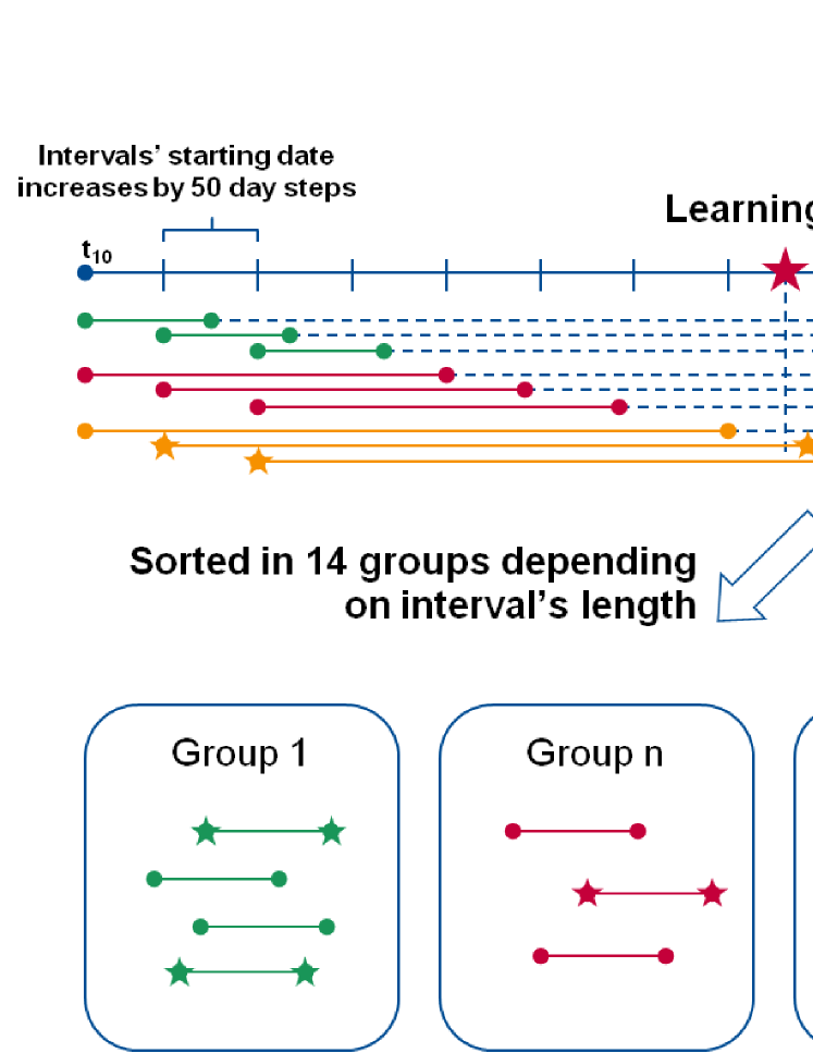
Figure 1: Step one of pattern recognition procedure: Create sub-windows, fit each window with the JLS model. Classify the fits in groups and classes.

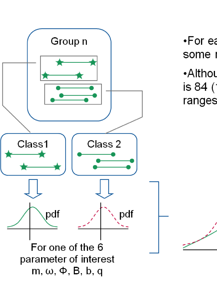
Figure 2: Step two of pattern recognition procedure: For each group compare fits in class I with those in class II and find out the informative parameters.

A figure is very helpful for understanding these concepts. We show the selection of the sub-windows and sort the fits by classes and groups in Fig. 1. Then we create the pdf’s of each of these parameters for each fit and define informative parameters as those parameters for which the pdf’s differ significantly according to a Kolmogorov-Smirnov test. For each informative parameter, we find the regions of the abscissa of the pdf for which the Class I pdf (fits with $t_{c}$ close to an extremum) is greater than the Class II pdf. This procedure has been performed in Fig. 2.

[Figs. 1–2 about here.]

III.4 Questionnaires, traits and features

Using the informative parameters and their pdf’s described above, we can generate a questionnaire for each day of the learning or testing set. A questionnaire is a quantitative inquiry into whether or not a set of parameters is likely to indicate a bubble or negative bubble. Questionnaires will be used to identify bubbles (negative bubbles) which will be followed by crashes (rebounds). In short, the length of a questionnaire tells how many informative parameters there are for a given window size. An informative parameter implies that the pdf’s of that parameter are very different for windows with a crash/rebound than windows without. The more values of ‘1’ in the questionnaire, the more likely it is that the parameters are associated with a crash/rebound.

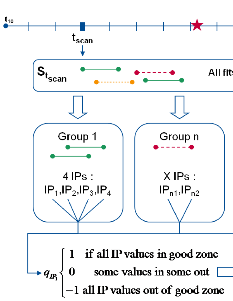
Figure 3: Step three of pattern recognition procedure: Generate the questionnaire for each trading day.

One questionnaire is constructed for each day $t_{scan}$ in our learning set. We first collect all the fits which have a critical time near that day (‘near’ will be defined). Then we create a string of bits whose length is equal to the number of informative parameters found. Each bit can take a value -1, 0 or 1 (a balanced ternary system). Each bit represents the answer to the question: are more than half of the collected fits more likely to be considered as Class I? If the answer is ‘yes’, we assign $1$ in the bit of the questionnaire corresponding to this informative parameter. Otherwise, we assign $0$ when the answer cannot be determined or $-1$ when the answer is ‘no’. A visual representation of this questionnaire process is shown in Fig. 3.

[Fig. 3 about here.]

The concept of a trait is developed to describe the property of the questionnaire for each $t_{scan}$. Each questionnaire can be decomposed into a fixed number of traits if the length of the questionnaire is fixed. We will not give the details in how the traits are generated in this paper. For a clear explanation of the method, please refer to Sec. 3.9 of the reference rebound . Think of a trait as a sub-set (like the ‘important’ short section from a very long DNA sequence) of a fixed-length questionnaire that is usually found in windows that show crashes/rebounds. Conversely, a trait can indicate windows where a crash/rebound is not found.

Assume that there are two sets of traits $T_{I}$ and $T_{II}$ corresponding to Class I and Class II, respectively. Scan day by day the date $t$ before the last day of the learning set. If $t$ is ‘near’ an extreme event (crash or rebound), then all traits generated by the questionnaire for this date belong to $T_{I}$. Otherwise, all traits generated by this questionnaire belong to $T_{II}$. ‘Near’ is defined as at most 20 days away from an extreme event. The same definition will be used later in Section IV when we introduce the error diagram.

Using this threshold, we declare that an alarm starts on the first day that the unsorted crash alarm index time series exceeds this threshold. The duration of this alarm $D_{a}$ is set to 41 days, since the longest distance between a crash and the day with index greater than the threshold is 20 days.

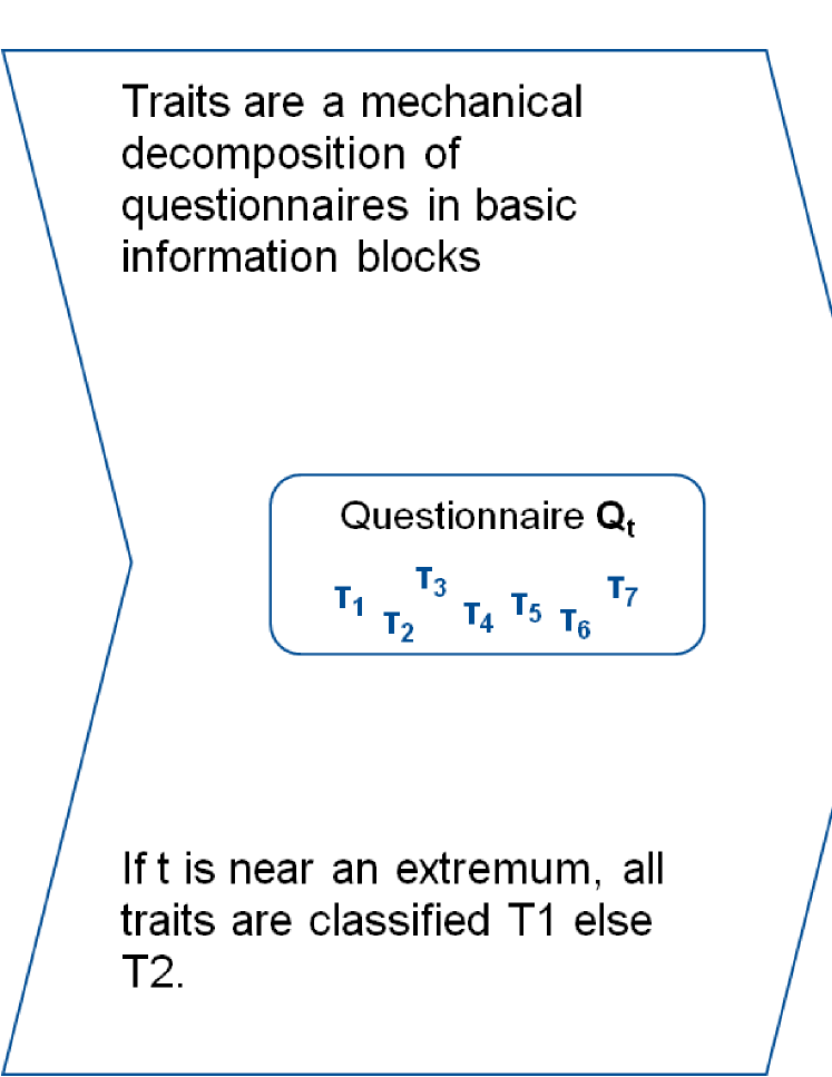
Figure 4: Step four of pattern recognition procedure: Create traits from questionnaires. Obtain features for each class by traits statistics.

Count the frequencies of a single trait $\tau$ in $T_{I}$ and $T_{II}$. If $\tau$ is in $T_{I}$ for more than $\alpha$ times and in $T_{II}$ for less than $\beta$ times, then we call this trait $\tau$ a feature $F_{I}$ of Class I. Similarly, if $\tau$ is in $T_{I}$ for less than $\alpha$ times and in $T_{II}$ for more than $\beta$ times, then we call $\tau$ a feature $F_{II}$ of Class II. The pair $(\alpha,\beta)$ is defined as a feature qualification. Fig. 4 shows the generation process of traits and features. We would like to clarify that by definition some of the traits are not from any type of feature since they are not ‘extreme’ and we cannot extract clear information from them.

[Fig. 4 about here.]

III.5 Alarm index

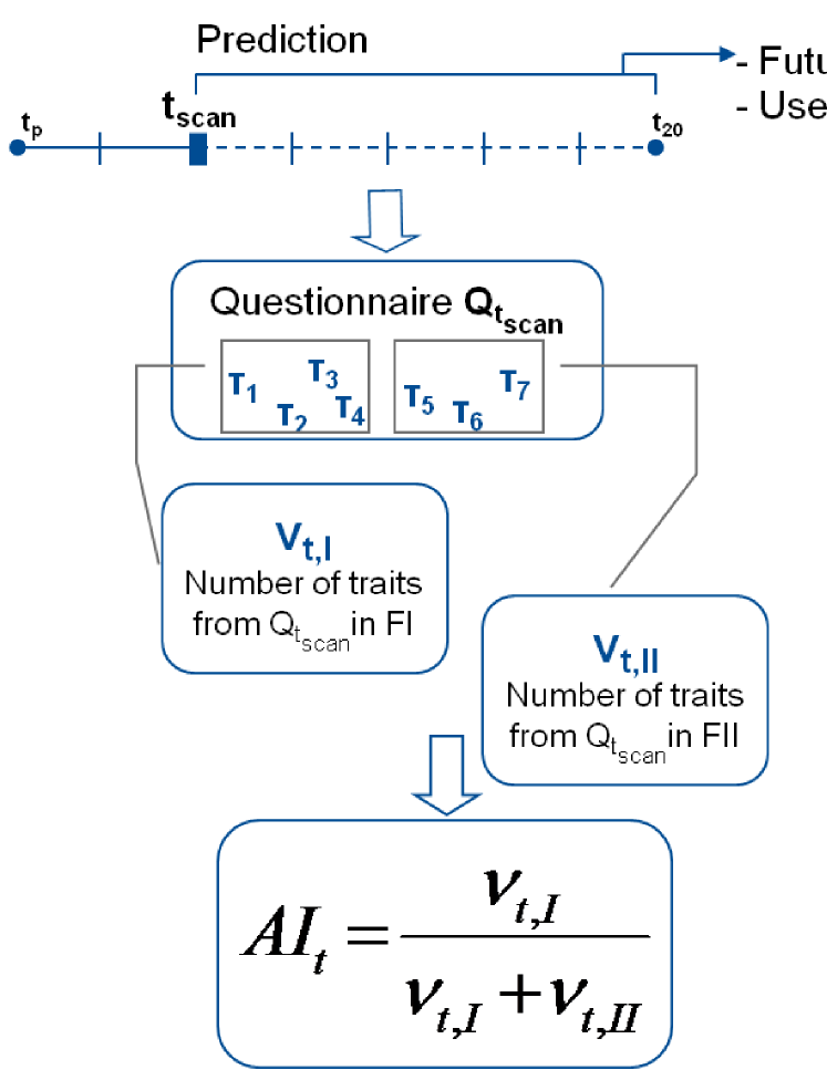
Figure 5: Step five of pattern recognition procedure: Construct the alarm index for each day by decomposing the questionnaire into traits for that day and compare these traits to the features of each class.

The final piece in our methodology is to define an alarm index for both crashes and rebounds. An alarm index is developed based on features to show the probability that a certain day is considered to be a rebound or a crash. We first collect all the fits which have a predicted critical time near this specific day and generate questionnaires and traits from these fits. The rebound (crash) alarm index for a certain day is just a ratio quantified by the total number of traits from feature type $F_{I}$ (a set of traits which have high probability to represent rebound (crash)) divided by the total number of traits from both $F_{I}$ and $F_{II}$. Note that $F_{II}$ is a set of traits which have low probability to represent rebound (crash). The principles for the generation of the alarm index are summarized in Fig. 5.

[Fig. 5 about here.]

Two types of alarm index are developed. One is for the back tests in the learning set, as we have already used the information before this time to generate informative parameters and features. The other alarm index is for the prediction tests. We generate this prediction alarm index using only the information before a certain time and then try to predict crashes and rebounds in the ‘future’.

IV Prediction in major equity markets

We perform systematic detections and forecasts on both the market crashes and rebounds for 10 major global equity markets using the method we discussed in Sec. III. The 10 indices are S&P 500 (US), Nasdaq composite (US), Russell 2000 (US), FTSE 100 (UK), CAC 40 (France), SMI (Switzerland), DAX (German), Nikkei 225 (Japan), Hang Seng (Hong Kong) and ASX (Australia). The basic information for these indices used in this study is listed in Tab. 1. Due to space constraints, we cannot show all results for these 10 indices here. The complete results for three indices from different continents are shown in this paper. They are Russell 2000 (America), SMI (Europe) and Nikkei 225 (Asia). Partial results for the remaining indices are shown in Tab. 2, which will be discussed in details later in Sec. V.

The alarm index depends on the features which are generated using information from the learning set. Thus, the alarm index before the end of the learning set uses ‘future’ information. That is, the value of the alarm index on a certain day $t_{0}$ in the learning set uses prices found at $t>t_{0}$ to generate features. The feature definitions from the learning set are then used to define the alarm index in the testing set using only past prices. That is, the value of the alarm index on a certain day $t_{0}$ in the testing set uses only prices found at $t\leq t_{0}$ in the testing set (and the definitions of features found in the learning set). We do not use ‘future’ information in the testing set. In this case, the alarm index predicts crashes and rebounds in the market.

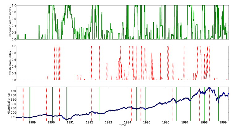
Figure 6: Alarm index and log-price of the Russell 2000 Index for the learning set, where the end date is 17-Apr-1999. (upper) Rebound alarm index for the learning set using feature qualification pair $(7,100)$. The rebound alarm index is in the range $[0,1]$. The higher the rebound alarm index, the more likely is the occurrence of a rebound. (middle) Crash alarm index for the learning set using feature qualification pair $(7,100)$. The crash alarm index is in the range $[0,1]$. The higher the crash alarm index, the more likely is the occurrence of a crash. (lower) Plot of price versus time of Russell Index (shown in blue cycles). Green solid vertical lines indicate rebounds defined by local minima within plus and minus 100 days around them. Red dashed vertical lines indicate crashes defined by local maxima within plus and minus 100 days around them. Note that these rebounds and crashes are the historical “change of regime” rather than only the jump-like reversals.

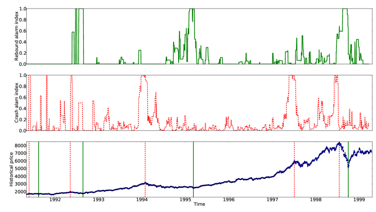
Figure 7: Alarm index and price of the SMI Index for the learning set, where the end date is 17-Apr-1999. The format is the same as Fig. 6.

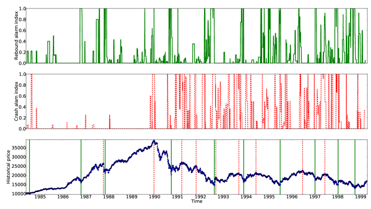
Figure 8: Alarm index and price of the Nikkei 225 Index for the learning set, where the end date is 17-Apr-1999. The format is the same as Fig. 6.

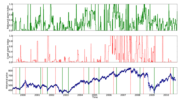
Figure 9: Alarm index and log-price of Russell 2000 Index for the predicting set after 17-Apr-1999. The format is the same as Fig. 6.

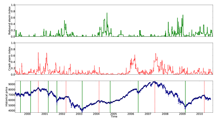
Figure 10: Alarm index and price of the SMI Index for the predicting set after 17-Apr-1999. The format is the same as Fig. 6.

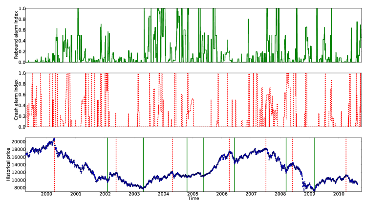
Figure 11: Alarm index and price of the Nikkei 225 Index for the predicting set after 17-Apr-1999. The format is the same as Fig. 6.

The crash and the rebound alarm index for Russell 2000, SMI and Nikkei are shown in Figs. 6–11. Figs. 6–8 show the back testing results for these three indices and Figs. 9–11 present the prediction results. In all of these results, the feature qualification pair $(7,100)$ is used. This means that a certain trait must appear in trait Class I (crash or rebound) at least 7 times and must appear in trait Class II (no crash or rebound) less than 100 times. If so, then we say that this trait is a feature of Class I. If, on the other hand, the trait appears 7 times or less in Class I or appears 100 times or more in Class II, then this trait is a feature of Class II. Tests on other feature qualification pairs are performed also. Due to the space constraints, we do not show the alarm index constructed by other feature qualification pairs here, but later we will present the predictability of these alarm indices by showing the corresponding error diagrams. In the rest of this paper, if we do not mention otherwise, we use $(7,100)$ as the feature qualification pair.

[Figs. 6–11 about here.]

To check the quality of the alarm index quantitatively, we introduce error diagrams Molchan1 ; Molchan2 . Using Nikkei 225 as an example, we create an error diagram for crash predictions after 17-Apr-1999 with a certain feature qualification in the following way:

1. Calculate features and define the alarm index using the learning set between 04-Jan-1984 and 17-Apr-1999.

2. Count the number of crashes after 17-Apr-1999 as defined in Sec. III.2 and expression (11). There are 7 crashes.

3. Take the crash alarm index time series (after 17-Apr-1999) and sort the set of all alarm index values in decreasing order. There are 4,141 points in this series and the sorting operation delivers a list of 4,141 index values, from the largest to the smallest one.

4. The largest value of this sorted series defines the first threshold.

5. Using this threshold, we declare that an alarm starts on the first day that the unsorted crash alarm index time series exceeds this threshold. The duration of this alarm $D_{a}$ is set to 41 days, since the longest distance between a crash and the day with index greater than the threshold is 20 days. This threshold is consistent with the previous classification of questionnaires in Section III.4, where we define a predicted critical time as ‘near’ the real extreme events when its distance is less than 20 days. Then, a prediction is deemed successful when a crash falls inside that window of 41 days.

6. If there are no successful predictions at this threshold, move the threshold down to the next value in the sorted series of alarm index.

7. Once a crash is predicted with a new value of the threshold, count the ratio of unpredicted crashes (unpredicted crashes / total crashes in set) and the ratio of alarms used (duration of alarm period / 4,141 prediction days). Mark this as a single point in the error diagram.

In this way, we will mark 7 points in the error diagram for the 7 Nikkei 225 crashes after 17-Apr-1999.

The aim of using such an error diagram in general is to show that a given prediction scheme performs better than random. A random prediction follows the line $y=1-x$ in the error diagram. A set of points below this line indicates that the prediction is better than randomly choosing alarms. The prediction is seen to improve as more error diagram points are found near the origin point $(0,0)$. The advantage of error diagrams is to avoid discussing how different observers would rate the quality of predictions in terms of the relative importance of avoiding the occurrence of false positive alarms and of false negative missed rebounds. By presenting the full error diagram, we thus sample all possible preferences and the unique criterion is that the error diagram curve be shown to be statistically significantly below the anti-diagonal $y=1-x$.

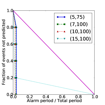
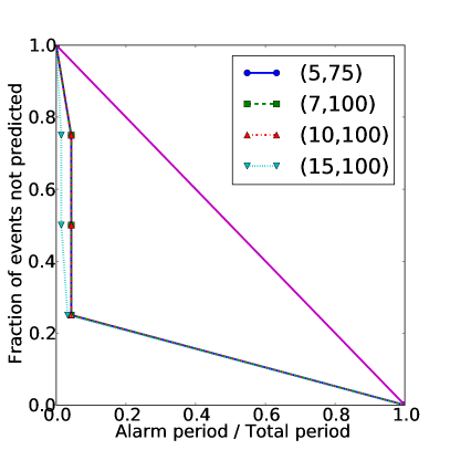
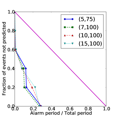
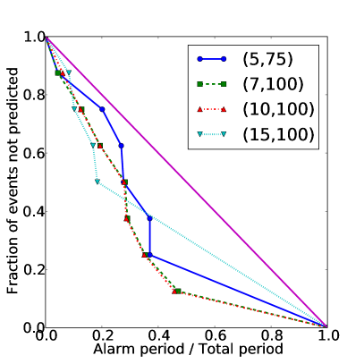
Figure 13: Error diagram for back tests and predictions of crashes and rebounds for SMI index with different types of feature qualifications. The format is the same as Fig. 12.

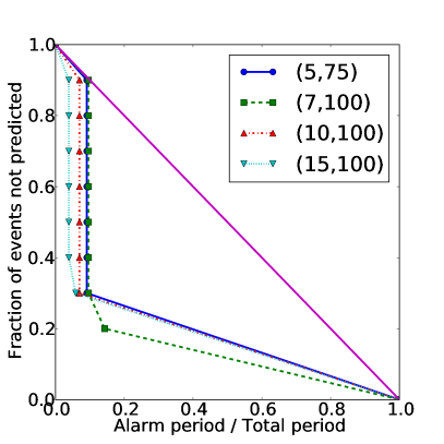
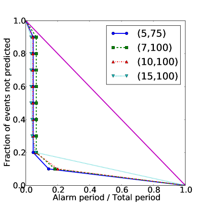
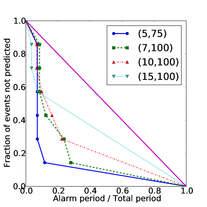
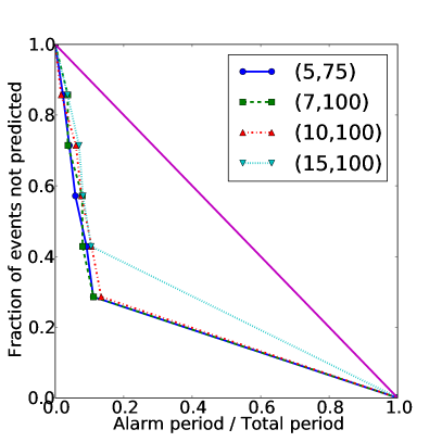
Figure 14: Error diagram for back tests and predictions of crashes and rebounds for Nikkei 225 index with different types of feature qualifications. The format is the same as Fig. 12.

In Figs. 12–14, we show the results on predictions and back tests in terms of error diagrams for crashes and rebounds in each of the indices. The results for different feature qualification pairs $(\alpha,\beta)$ are shown in each figure. All these figures show that our alarm index for crashes and rebounds in either back testing or prediction performs much better than random.

[Figs. 12–14 about here.]

V Trading Strategy

One of the most powerful methods to test the predictability of a signal is to design simple trading strategies based on it. We do so with our alarm index by using simple moving average strategies, which keep all the key features of the alarm index and avoid parametrization problems. The strategies are kept as simple as possible and can be applied to any indices.

The trading strategies are designed as follows: the daily exposure of our strategy $\theta$ is determined by the average value of the alarm index for the past $n$ days. The rest of our wealth, $1-\theta$, is invested in a 3-month US treasury bill.

Let us denote the average rebound and crash alarm index of the past $n$ days as $AI_{R}$ and $AI_{C}$ respectively. We create three different strategies:

• A long strategy using only the rebound alarm index. We will take a long position in this strategy only. The daily exposure of our strategy is based on the average value of the past $n$ days rebound alarm index: $\theta=AI_{R}$.

• A short strategy using only the crash alarm index. We will take a short position in this strategy only. The daily absolute exposure of our strategy is based on the average value of the past $n$ days crash alarm index: $|\theta|=AI_{C}$.

• A long-short strategy linearly combining both strategies above. When the average rebound alarm index is higher than the average crash alarm index, we take a long position and vice versa. The absolute exposure $|\theta|=|AI_{R}-AI_{C}|$.

These strategies have the advantage of having few parameters, as only the duration $n$ needs to be determined. Despite their simplicity, they capture the two key features of the alarm index. First, we see that the alarms are clustered around certain dates. The more clustering seen, the more likely that a change of regime is coming and, therefore, the more we should be invested. Second, we see that a strong alarm close to $1$ should be treated as more important than a weaker alarm while at the same time the smaller alarms still contain some information and should not be discarded.

Tab. 2 summarizes the Sharpe ratios for long-short strategies on the out-of-sample period (testing set) for each index. The strategy is calculated with four different moving average look-backs: $n=20,30,40,60$ days. We use the Sharpe ratios of the market during this period as the benchmark in this table. Recall that the Sharpe ratio is a measure of the excess return (or risk premium) per unit of risk in an investment asset or a trading strategy. It is defined as:

$$S=\frac{R-R_{f}}{\sigma}=\frac{R-R_{f}}{\sqrt{Var[R-R_{f}]}}~{},$$ (13)

where $R$ is the return of the strategy and $R_{f}$ is the risk free rate. We use the US three-month treasury bill rate here as the risk free rate. The Sharpe ratio is used to characterize how well the return of an asset compensates the investor for the risk taken: the higher the Sharpe ratio number, the better. When comparing two assets with the same expected return against the same risk free rate, the asset with the higher Sharpe ratio gives more return for the same risk. Therefore, investors are often advised to pick investments with high Sharpe ratios. From Tab. 2, we can find that, for seven out of ten global major indices, the Sharpe ratios of our strategies (no matter which look-back duration $n$ is chosen) are much higher than the market, which means that our strategies perform better than the simple buy and hold strategy. This result indicates that the JLS model combined with the pattern recognition method has a statistically significant power in systematic detection of rebounds and of crashes in financial markets.

[Tab. 2 about here.]

The long-short strategies for CAC 40, DAX and ASX perform not as well as the market. However, this is not a statement against the prediction power of our method, but instead supports the evidence that our method detects specific signatures preceding rebounds and crashes that are essentially different from high volatility indicators. Contrary to common lore and to some exceptional empirical cases schwert_stock_1990 ; AndersenSor04 , crashes of the financial markets often happen during low-volatility periods and terminate them. By construction, both our rebound alarm index and the crash alarm index are high during such volatile periods. So if the alarm indices of both types are high at the same time, it is likely that the market is experiencing a highly volatile period. Now, we can refine the strategy and combine the evidence of a directional crash or rebound, together with a high volatility indicator. If we interpret the two co-existing evidences as a signal for a crash, we should ignore these rebound alarm index and take the short strategy mentioned before. As an application, we show the wealth trajectories of DAX based on different type of strategies in Fig. 15. In the beginning of 2008, both the rebound alarm index and the crash alarm index for DAX are very high, therefore, we detect this period as a highly volatile period and ignore the rebound alarm index. The short strategy gives a very high Sharpe ratio $S=0.41$ compared to the long-short and short benchmarks where $S=0.06$. The strategy’s average weight is used to compute these benchmarks. These simple benchmarks are constantly invested by a given percentage in the market so that, over the whole time period, they give the same exposure as the corresponding strategy being tested but without the genuine timing information the strategy should contain.

[Figs. 15 about here.]

As before, the detailed out-of-sample performances for each sample index (Russell 2000, SMI and Nikkei 225) are also tested. Fig. 16–18 illustrate the wealth trajectories for different strategies. In order to show the consistency of the strategies with respect to the chosen parameters in the pattern recognition method, we show the performance of the Russell 2000 index for different qualification pairs: $(15,100)$ for rebounds and $(10,100)$ for crashes. From these wealth trajectories, it is very obvious that our alarm indices can catch the market rebounds and crashes efficiently.

[Figs. 16–18 about here.]

The detailed performances for these three stock indices are listed in Tabs. 3–6. We also provide the performance of the Russell 2000 index for the ‘normal’ qualification pair: $(7,100)$ in Tab. 4 as a reference. These tables confirm again that strategies mostly succeed in capturing big changes of regime. Compared to the market, the strategies based on our alarm index perform better than the market for more than eleven years in all the important measures: Annual returns and Sharpe ratios are larger, while volatilities, downside deviations and maximum drawdowns are smaller than the market performance.

[Tabs. 3–6 about here.]

VI Conclusion

We provided a systematic method to detect financial crashes and rebounds. The method is a combination of the JLS model for bubbles and negative bubbles, and the pattern recognition technique originally developed for earthquake predictions. The outcome of this method is a rebound/crash alarm index to indicate the probability of a rebound/crash for a certain time. The predictability of the alarm index has been tested by 10 major global stock indices. The performance is checked quantitatively by error diagrams and trading strategies. All the results from error diagrams indicate that our method in detecting crashes and rebounds performs better than chance and confirm that the new method is very powerful and robust in the prediction of crashes and rebounds in financial markets. Our long-short trading strategies based on the crash and rebound alarm index perform better than the benchmarks (buy and hold strategy with the same exposure as the average exposure of our strategies) in seven out of ten indices. Highly volatile periods are observed in the indices of which the long-short trading strategy fails to surpass the benchmark. By construction of the alarm index and the fact that highly volatile periods are not coherent with bullish markets, we claim that we should ignore the rebound alarm index during such volatile periods. This statement has been proved by the short strategy which only consider the crash alarm index. Thus, our trading strategies confirm again that the alarm index has a strong ability in detecting rebounds and crashes in the financial markets.

Reference

Index name	Yahoo ticker	Learning start	Prediction start	Prediction end	win. #
S&P 500	^GSPC	5-Jan-1950	26-Mar-1999	3-Jun-2009	11662
Nasdaq	^IXIC	13-Dec-1971	20-Mar-1999	30-Jul-2010	7209
Russell 2000	^RUT	30-Sep-1987	17-Apr-1999	27-Aug-2010	4270
FTSE 100	^FTSE	3-May-1984	17-Apr-1999	27-Aug-2010	4970
CAC 40	^FCHI	1-Mar-1990	17-Apr-1999	27-Aug-2010	3766
SMI	^SSMI	9-Nov-1990	17-Apr-1999	27-Aug-2010	3626
DAX	^GDAXI	26-Nov-1990	17-Apr-1999	27-Aug-2010	3626
Nikkei 225	^N225	4-Jan-1984	17-Apr-1999	27-Aug-2010	5026
Hang Seng	^HSI	31-Dec-1986	17-Apr-1999	27-Aug-2010	4410
ASX	^AORD	6-Aug-1984	17-Apr-1999	27-Aug-2010	4914

Table 1: Information for the tested indices: Yahoo ticker of each index, starting time of learning and prediction periods, ending time of prediction and number of sub-windows.

Index	Strategy (duration $n$)				Market
	20	30	40	60
S&P 500	0.32	0.38	0.43	0.39	-0.28
Nasdaq	0.18	0.41	0.48	0.34	-0.11
Russell 2000	0.29	0.3	0.27	0.27	0.03
FTSE 100	-0.07	-0.06	0.01	0.05	-0.22
CAC 40	-0.18	-0.35	-0.37	-0.24	-0.19
SMI	0.28	0.22	0.14	0.13	-0.20
DAX	-0.26	-0.24	-0.27	-0.19	-0.06
Nikkei 225	0.07	0.19	0.39	0.59	-0.33
Hang Seng	0.32	0.38	0.31	0.23	0.06
ASX	-0.38	-0.41	-0.33	-0.24	0.02

Table 2: Summary of Sharpe ratios for the market and the long-short strategies with different moving average duration $n$. The start and end dates of the strategies are 26-Mar-1999 – 3-Jun-2009 for S&P 500, 20-Mar-1999 – 30-Jul-2010 for Nasdaq and 17-Apr-1999 – 27-Aug-2010 for others. The feature qualification pairs of $(7,100)$ for both crash and rebound alarm indices are used in this calculation.

	Strategy (duration $n$)				Market
	20	30	40	60
Ann Ret	5.3%	5.4%	4.8%	4.2%	0.1%
Vol	6.4%	5.9%	5.3%	4.1%	26.3%
Downside dev	4.2%	3.6%	3.4%	2.7%	18.9%
Sharpe	0.42	0.47	0.41	0.37	0.03
Max DD	10%	7%	7%	6%	65%
Abs Expo	16%	15%	14%	12%
Ann turnover	328%	220%	167%	123%

Table 3: Russell 2000 index long-short strategies out-of-sample performance table. Start date: 17-Apr-1999, end date 27-Aug-2010. Qualification pairs: $(15,100)$ for rebounds and $(10,100)$ for crashes.

	Strategy (duration $n$)				Market
	20	30	40	60
Ann Ret	4.8%	4.7%	4.3%	4.0%	0.1%
Vol	7.9%	7.1%	6.5%	5.2%	26.3%
Downside dev	5.4%	4.8%	4.5%	3.6%	18.9%
Sharpe	0.29	0.30	0.27	0.27	0.03
Max DD	11%	12%	9%	9%	65%
Abs Expo	23%	21%	20%	18%
Ann turnover	446%	306%	237%	172%

Table 4: Russell 2000 index long-short strategies out-of-sample performance table. Start date: 17-Apr-1999, end date 27-Aug-2010. Qualification pairs: $(7,100)$ for both rebounds and crashes.

	Strategy (duration $n$)				Market
	20	30	40	60
Ann Ret	3.4%	3.3%	3.0%	3.0%	-3.4%
Vol	2.6%	2.6%	2.5%	2.3%	20.4%
Downside dev	1.7%	1.6%	1.6%	1.5%	14.6%
Sharpe	0.28	0.22	0.14	0.13	-0.20
Max DD	7%	6%	7%	5%	59%
Abs Expo	9%	9%	9%	9%
Ann turnover	134%	102%	77%	55%

Table 5: SMI index long-short strategies out-of-sample performance table. Start date 17-Apr-1999, end date 27-Aug-2010.

	Strategy (duration $n$)				Market
	20	30	40	60
Ann Ret	3.0%	3.7%	4.8%	5.7%	-8.4%
Vol	6.3%	6.0%	5.6%	5.0%	25.4%
Downside dev	4.4%	4.1%	3.7%	3.2%	18.7%
Sharpe	0.07	0.19	0.39	0.59	-0.33
Max DD	15%	13%	10%	8%	75%
Abs Expo	19%	18%	17%	16%
Ann turnover	417%	300%	223%	146%

Table 6: Nikkei 225 index long-short strategies out-of-sample performance table. Start date 17-Apr-1999, end date 27-Aug-2010.

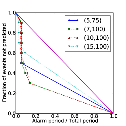
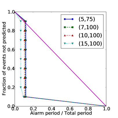
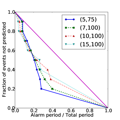
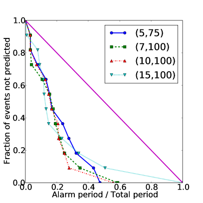
Figure 12: Error diagram for back tests and predictions of crashes and rebounds for Russell 2000 index with different types of feature qualifications. The value of the feature qualifications are shown in the legend. The fact that all the curves lie under the line $y=1-x$ indicates better performance than chance in detecting crashes and rebounds using our method.
(Upper left) Back tests of crashes. (Upper right) Back tests of rebounds. (Lower left) Predictions of crashes. (Lower right) Predictions of rebounds. Feature qualification $(\alpha,\beta)$ means that, if the occurrence of a certain trait in Class I is larger than $\alpha$ and less than $\beta$, then we call this trait a feature of Class I and vice versa. See text for more information.

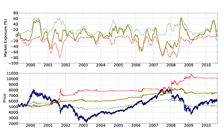
Figure 15: Performance of trading strategy using our technique: DAX index 60 days moving average strategy using the feature qualification pair $(15,100)$ for crashes and $(10,200)$ for rebounds. (upper) the exposures for different strategies, where the olive solid line represents the long-short strategy, the green dotted line and red dashed line are for long and short strategy respectively. (Lower) The historical price and wealth trajectories of the strategies. The blue circles represent the historical price of the index while the others are the wealth trajectories consistent with the upper figure (olive solid - long-short, green dotted - long, red dashed - short).
The Sharpe ratio for the strategies are $0.07$ (long-short), $-0.66$ (long) and $0.41$ (short). The Sharpe ratio of the corresponding benchmarks, which consist of constant position in the market with exposure equal to the strategy over the whole period, are $0.06$ (long-short), $-0.06$ (long) and $0.06$ (short). And the Sharpe ratio of the index in this period is $-0.06$. Note that the short strategy performs better than long-short or long strategies as discussed in the text.

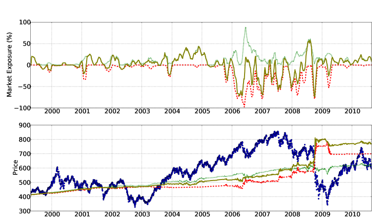
Figure 16: Performance of trading strategy using our technique: Russell 2000 index 30 days moving average strategy using the feature qualification pair $(15,100)$ for crashes and $(10,100)$ for rebounds. The format is the same as Fig. 15.
The Sharpe ratio for the strategies are $0.47$ (long-short), $0.18$ (long) and $0.26$ (short). The Sharpe ratio of the corresponding benchmarks, which consist of constant position in the market with exposure equal to the strategy over the whole period, are $0.03$ (long-short), $0.03$ (long) and $-0.03$ (short). And the Sharpe ratio of the index in this period is $0.03$.

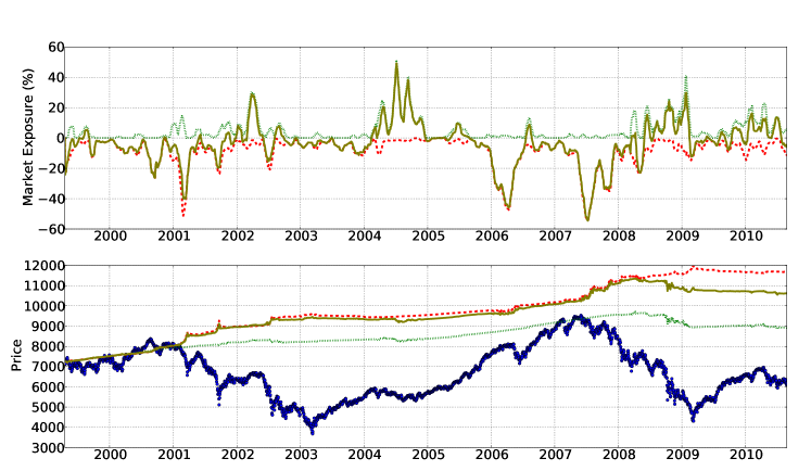
Figure 17: Performance of trading strategy using our technique: SMI index 20 days moving average strategy. The format is the same as Fig. 15.
The Sharpe ratio for the strategies are $0.28$ (long-short), $-0.04$ (long) and $0.65$ (short). The Sharpe ratio of the corresponding benchmarks, which consist of constant position in the market with exposure equal to the strategy over the whole period, are $0.2$ (long-short), $-0.2$ (long) and $0.2$ (short). And the Sharpe ratio of the index in this period is $-0.2$.

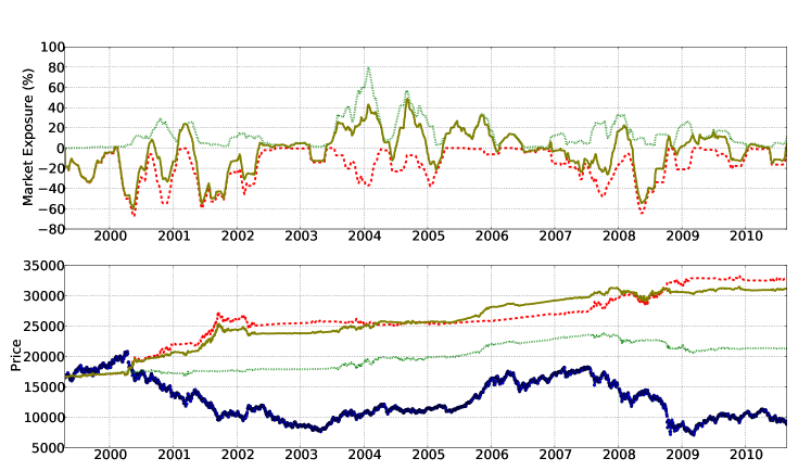
Figure 18: Performance of trading strategy using our technique: Nikkei 225 index 60 days moving average strategy. The format is the same as Fig. 15.
The Sharpe ratio for the strategies are $0.59$ (long-short), $-0.11$ (long) and $0.59$ (short). The Sharpe ratio of the corresponding benchmarks, which consist of constant position in the market with exposure equal to the strategy over the whole period, are $0.33$ (long-short), $-0.33$ (long) and $0.33$ (short). And the Sharpe ratio of the index in this period is $-0.33$.

References

- (1) T. Kaizoji, D. Sornette, Market bubbles and crashes, in: the Encyclopedia of Quantitative Finance, Wiley, 2009, long version at http://arxiv.org/abs/0812.2449.
- (2) A. Johansen, O. Ledoit, D. Sornette, Crashes as critical points, International Journal of Theoretical and Applied Finance 3 (2000) 219–255.
- (3) A. Johansen, D. Sornette, O. Ledoit, Predicting financial crashes using discrete scale invariance, Journal of Risk 1 (4) (1999) 5–32.
- (4) A. Johansen, D. Sornette, Critical crashes, Risk 12 (1) (1999) 91–94.
- (5) D. Sornette, Why Stock Markets Crash (Critical Events in Complex Financial Systems), Princeton University Press, 2003.
- (6) K. Watanabe, H. Takayasu, M. Takayaso, A mathematical definition of the financial bubbles and crashes, Physica A 383 (1) (2007) 120–124.
- (7) D. Abreu, M. K. Brunnermeier, Bubbles and crashes, Econometrica 71(1) (2003) 173–204.
- (8) W. Yan, R. Woodard, D. Sornette, Diagnosis and prediction of market rebounds in financial markets, http://arxiv.org/abs/1001.0265 (2010).
- (9) W. Yan, R. Woodard, D. Sornette, Diagnosis and prediction of tipping points in financial markets: Crashes and rebounds, Physics Procedia 3 (2010) 1641–1657.
- (10) D. Sornette, R. Woodard, W.-X. Zhou, The 2006-2008 oil bubble: Evidence of speculation and prediction, Physica A 388 (2009) 1571–1576.
- (11) Z.-Q. Jiang, W.-X. Zhou, D. Sornette, R. Woodard, K. Bastiaensen, P. Cauwels, Bubble diagnosis and prediction of the 2005-2007 and 2008-2009 Chinese stock market bubbles, Journal of Economic Behavior and Organization 74 (2010) 149–162.
- (12) W.-X. Zhou, D. Sornette, Analysis of the real estate market in Las Vegas: Bubble, seasonal patterns, and prediction of the CSW indexes, Physica A 387 (2008) 243–260.
- (13) W.-X. Zhou, D. Sornette, 2000-2003 real estate bubble in the UK but not in the USA, Physica A 329 (2003) 249–263.
- (14) W.-X. Zhou, D. Sornette, Is there a real estate bubble in the US?, Physica A 361 (2006) 297–308.
- (15) A. Johansen, D. Sornette, Financial “anti-bubbles”: log-periodicity in gold and Nikkei collapses, International Journal of Modern Physics C 10 (4) (1999) 563–575.
- (16) D. Sornette, W.-X. Zhou, The US 2000-2002 market descent: How much longer and deeper?, Quantitative Finance 2 (6) (2002) 468–481.
- (17) N. Vandewalle, M. Ausloos, P. Boveroux, A. Minguet, Visualizing the log-periodic pattern before crashes, European Physics Journal B 9 (1999) 355–359.
- (18) A. Clark, Evidence of log-periodicity in corporate bond spreads, Physica A 338 (2004) 585–595.
- (19) P. Gnaciński, D. Makowiec, Another type of log-periodic oscillations on Polish stock market, Physica A 344 (2004) 322–325.
- (20) M. Bartolozzi, S. Drożdż, D. Leinweber, J. Speth, A. Thomas, Self-similar log-periodic structures in Western stock markets from 2000, International Journal of Modern Physics C 16 (2005) 1347–1361.
- (21) R. Matsushita, S. da Silva, A. Figueiredo, I. Gleria, Log-periodic crashes revisited, Physica A 364 (2006) 331–335.
- (22) S. Drożdż, J. Kwapień, P. Oświecimka, J. Speth, Current log-periodic view on future world market development, Acta Physica Polonica A 114 (2008) 539–546.
- (23) W.-X. Zhou, D. Sornette, A case study of speculative financial bubbles in the South African stock market 2003-2006, Physica A 388 (2009) 869–880.
- (24) W. Yan, R. Woodard, D. Sornette, Leverage bubble, Physica A, forthcoming. http://arxiv.org/abs/1011.0458 (2011).
- (25) D. Sornette, R. Woodard, M. Fedorovsky, S. Reimann, H. Woodard, W.-X. Zhou, The financial bubble experiment: Advanced diagnostics and forecasts of bubble terminations (the financial crisis observatory), http://arxiv.org/abs/0911.0454 (2010).
- (26) D. Sornette, R. Woodard, M. Fedorovsky, S. Reimann, H. Woodard, W.-X. Zhou, The financial bubble experiment: Advanced diagnostics and forecasts of bubble terminations volume II (master document), http://arxiv.org/abs/1005.5675 (2010).
- (27) R. Woodard, D. Sornette, M. Fedorovsky, The financial bubble experiment: Advanced diagnostics and forecasts of bubble terminations volume III (beginning of experiment + post-mortem analysis), http://arxiv.org/abs/1011.2882 (2011).
- (28) D. Sornette, W.-X. Zhou, Predictability of large future changes in major financial indices, International Journal of Forecasting 22 (2006) 153–168.
- (29) P. L. Briggs, F. Press, Pattern recognition applied to uranium prospecting, Nature 268 (5616) (1977) 125–127.
- (30) V. Keilis-Borok, A. Soloviev, C. Allègre, A. Sobolevskii, M. Intriligator, Patterns of macroeconomic indicators preceding the unemployment rise in western europe and the USA, Pattern Recognition 38 (3) (2005) 423–435.
- (31) O. Blanchard, M. Watson, Bubbles, rational expectations and speculative markets, NBER Working Paper 0945, http://papers.ssrn.com/sol3/papers.cfm?abstract_id=226909 (1983).
- (32) D. Sornette, Discrete scale invariance and complex dimensions, Physics Reports 297 (5) (1998) 239–270.
- (33) H.-C. G. van Bothmer, C. Meister, Predicting critical crashes? A new restriction for the free variables, Physica A 320 (2003) 539–547.
- (34) I. M. Gelfand, S. A. Guberman, V. I. Keilis-Borok, L. Knopoff, F. Press, E. Y. Ranzman, I. M. Rotwain, A. M. Sadovsky, Pattern recognition applied to earthquake epicenters in california, Physics of The Earth and Planetary Interiors 11 (3) (1976) 227–283.
- (35) G. M. Mochan, Earthquake prediction as a decision making problem, Pure and Applied Geophysics 149 (1997) 233–247.
- (36) G. M. Mochan, Y. Y. Kagan, Earthquake prediction and its optimization, Journal of Geophysical Research 97 (1992) 4823–4838.
- (37) G. Schwert, Stock volatility and the crash of ’87, Review of Financial Studies 3 (1) (1990) 77 –102.
- (38) J. V. Andersen, D. Sornette, Fearless versus fearful speculative financial bubbles, Physica A 337 (1–2) (2004) 565–585.