Three-component Fermi gas with SU(3) symmetry:
BCS-BEC crossover in three and two dimensions

Abstract

We analyze the crossover from the Bardeen-Cooper-Schrieffer (BCS) state of weakly bound Fermi pairs to the Bose-Einstein condensate (BEC) of molecular dimers for a Fermi gas made of neutral atoms in three hyperfine states with a SU(3) invariant attractive interaction. By solving the extended BCS equations for the total number of particles and the pairing gap, we calculate at zero temperature the pairing gap, the population imbalance, the condensate fraction and the first sound velocity of the uniform system as a function of the interaction strength in both three and two dimensions. Contrary to the three-dimensional case, in two dimensions the condensate fraction approaches the value $1$ only for an extremely large interaction strength and, moreover, the sound velocity gives a clear signature of the disappearance of one of the three hyperfine components.

I Introduction

In the last years degenerate ultracold gases made of bosonic or fermionic atoms have been the subject of intense experimental and theoretical research book1 ; book2 . Among the several hot topics recently investigated, let us remind the expansion of a Fermi superfluid in the crossover from the Bardeen-Cooper-Schrieffer (BCS) state of weakly bound Fermi pairs to the Bose-Einstein condensate (BEC) of molecular dimers sigh07a ; sigh07b ; the surface effects in the unitary Fermi gas sigh10a ; the localization of matter waves in optical lattices sigh10b ; the transition to quantum turbolence in finite-size superfluids sigh10c ; sigh11 .

Very recently degenerate three-component gases have been experimentally realized using the three lowest hyperfine states of ⁶Li selim ; hara . At high magnetic fields the scattering lengths of this three-component system are very close each other and the system is approximately SU(3) invariant. Moreover, it has been theoretically predicted that good $SU(N)$ invariance (with $N\leq 10$) can be reached with ultracold alkaline-earth atoms (e.g. with ⁸⁷Sr atoms) wu1 ; wu2 ; ana . In the past various authors various1 ; various2 ; various3 ; various4 have considered the BCS regime of a fermionic gas with SU(3) symmetry. In the last years He, Jin and Zhang cinesi and Ozawa and Baym baym have investigated the full BCS-BEC crossover eagles ; leggett ; randeria ; marini ; sigh08 of this system at zero and finite temperature in three-dimensional space. Recently we have calculated the condensate fraction and the population imbalance for this three-component quantum gas both in the three-dimensional case and in the two-dimensional one iome . In this paper we review the extended BEC theory leggett ; randeria ; marini for an atomic gas with three-component fermions at zero temperature cinesi ; baym ; iome but without invoking functional integration. We obtain the chemical potential, the energy gap, the number densities and the condensate fraction as a function of the adimensional interaction strength. Finally, we calculate also the first sound velocity of the system both in three and two dimensions. In two dimensions we find that the sound velocity shows a kink at the critical strength (scaled binding energy) where one of the three hyperfine components goes to zero.

The Lagrangian density of a dilute and ultracold three-component uniform Fermi gas of neutral atoms is given by

$${\hat{\cal L}}=\sum_{\alpha=R,G,B}{\hat{\psi}}^{+}_{\alpha}\left(i\hbar{\partial\over\partial t}+{\hbar^{2}\over 2m}\nabla^{2}+\mu\right){\hat{\psi}}_{\alpha}-g\left({\hat{\psi}}^{+}_{R}{\hat{\psi}}^{+}_{G}{\hat{\psi}}_{G}{\hat{\psi}}_{R}+{\hat{\psi}}^{+}_{R}{\hat{\psi}}^{+}_{B}{\hat{\psi}}_{B}{\hat{\psi}}_{R}+{\hat{\psi}}^{+}_{G}{\hat{\psi}}^{+}_{B}{\hat{\psi}}_{B}{\hat{\psi}}_{G}\right)\;,$$ (1)

where ${\hat{\psi}}_{\alpha}({\bf r},t)$ is the field operator that destroys a fermion of component $\alpha$ in the position ${\bf r}$ at time $t$, while ${\hat{\psi}}_{\alpha}^{+}({\bf r})$ creates a fermion of component $\alpha$ in ${\bf r}$ at time $t$. To mimic QCD the three components are thought as three colors: red (R), green (G) and blue (B). The attractive inter-atomic interaction is described by a contact pseudo-potential of strength $g$ ($g<0$). The average total number of fermions is given by

$$N=\sum_{\alpha=R,G,B}\int\langle{\hat{\psi}}^{+}_{\alpha}({\bf r},t){\hat{\psi}}_{\alpha}({\bf r},t)\rangle\,d^{3}{\bf r}\;,$$ (2)

where $\langle\cdot\cdot\cdot\rangle$ is the ground-state average. Note that $N$ is fixed by the chemical potential $\mu$ which appears in Eq. (1). As stressed in Refs. cinesi ; baym , by fixing only the total chemical potential $\mu$ (or equivalently only the total number of atoms $N$) the Lagrangian (1) is invariant under global SU(3) rotations of the species.

II Extended BCS equations

At zero temperature the attractive interaction leads to pairing of fermions which breaks the SU(3) symmetry but only two colors are paired and one is left unpaired cinesi ; baym ; iome . We assume, without loss of generality cinesi ; baym ; iome , that the red and green particles are paired and the blue are not paired. The interacting terms can be then treated within the minimal mean-field BCS approximation, i.e. neglecting the Hartree terms while the pairing gap

$$\Delta=g\,\langle{\hat{\psi}}_{G}({\bf r},t){\hat{\psi}}_{R}({\bf r},t)\rangle$$ (3)

between red and green fermions is the key quantity. In this way the mean-field Lagrangian density becomes

$${\hat{\cal L}}_{mf}=\sum_{\alpha=R,G,B}{\hat{\psi}}^{+}_{\alpha}\left(i\hbar{\partial\over\partial t}+{\hbar^{2}\over 2m}\nabla^{2}+\mu\right){\hat{\psi}}_{\alpha}+\Delta\,{\hat{\psi}}_{G}{\hat{\psi}}_{R}+\Delta\,{\hat{\psi}}_{G}^{+}{\hat{\psi}}_{R}^{+}\;,$$ (4)

under the simplifying condition that the pairing gap is real, i.e. $\Delta^{*}=\Delta$. It is then straightforward to write down the Heisenberg equations of motion of the field operators:

$$i\hbar{\partial\over\partial t}{\hat{\psi}}_{R} = \left(-{\hbar^{2}\over 2m}\nabla^{2}-\mu\right){\hat{\psi}}_{R}+\Delta\,{\hat{\psi}}_{G}^{+}\;,$$ (5)

$$i\hbar{\partial\over\partial t}{\hat{\psi}}_{G} = \left(-{\hbar^{2}\over 2m}\nabla^{2}-\mu\right){\hat{\psi}}_{G}+\Delta\,{\hat{\psi}}_{R}^{+}\;,$$ (6)

$$i\hbar{\partial\over\partial t}{\hat{\psi}}_{B} = \left(-{\hbar^{2}\over 2m}\nabla^{2}-\mu\right){\hat{\psi}}_{B}\;,$$ (7)

which are coupled by the presence of the same chemical potential $\mu$ in the three equations. We now use the Bogoliubov-Valatin representation of the field operator ${\hat{\psi}}_{\alpha}({\bf r},t)$ in terms of the anticommuting quasi-particle Bogoliubov operators ${\hat{b}}_{{\bf k}\alpha}$:

$${\hat{\psi}}_{R}({\bf r},t) = \sum_{\bf k}\left(u_{k}e^{i({\bf k}\cdot{\bf r}-\omega_{k}t)}\,{\hat{b}}_{{\bf k}R}-v_{k}e^{-i({\bf k}\cdot{\bf r}-\omega_{k}t)}\,{\hat{b}}_{{\bf k}G}^{+}\right)\;,$$ (8)

$${\hat{\psi}}_{G}({\bf r},t) = \sum_{\bf k}\left(u_{k}e^{i({\bf k}\cdot{\bf r}-\omega_{k}t)}\,{\hat{b}}_{{\bf k}G}+v_{k}e^{-i({\bf k}\cdot{\bf r}-\omega_{k}t)}\,{\hat{b}}_{{\bf k}R}^{+}\right)\;,$$ (9)

$${\hat{\psi}}_{B}({\bf r},t) = \sum_{\bf k}e^{i({\bf k}\cdot{\bf r}-\Omega_{k}t)}\,{\hat{b}}_{{\bf k}B}\;,$$ (10)

where $u_{k}$ and $v_{k}$ are such that $u_{k}^{2}+v_{k}^{2}=1$. After inserting these expressions into the Heisenberg equations of motion of the field operators we get

$$\xi_{k} = \hbar\Omega_{k}={\hbar^{2}k^{2}\over 2m}-\mu\;,$$ (11)

$$E_{k} = \hbar\omega_{k}=\sqrt{\xi_{k}^{2}+\Delta^{2}}\;,$$ (12)

and also

$$u_{k}^{2}={1\over 2}\left(1+\frac{\xi_{k}}{E_{k}}\right)\;,\quad\quad\quad v_{k}^{2}={1\over 2}\left(1-\frac{\xi_{k}}{E_{k}}\right)\,.$$ (13)

By imposing the following ground-state averages

$$\langle{\hat{b}}_{{\bf k}B}^{+}{\hat{b}}_{{\bf k}^{\prime}B}\rangle=\Theta(-\xi_{k})\ \delta_{{\bf k},{\bf k}^{\prime}}\;,\quad\quad\langle{\hat{b}}_{{\bf k}R}^{+}{\hat{b}}_{{\bf k}R}\rangle=\langle{\hat{b}}_{{\bf k}G}^{+}{\hat{b}}_{{\bf k}G}\rangle=\Theta(-E_{k})\ \delta_{{\bf k},{\bf k}^{\prime}}\;,$$ (14)

with $\Theta(x)$ the Heaviside step function, the number equation (2) gives

$$N=N_{R}+N_{G}+N_{B}\;,$$ (15)

where

$$N_{R}=N_{G}={1\over 2}\sum_{\bf k}v_{k}^{2}$$ (16)

and

$$N_{B}=\sum_{\bf k}\Theta\left(\mu-{\hbar^{2}k^{2}\over 2m}\right)\;.$$ (17)

Similarly, the gap equation (3) gives

$$-{1\over g}={1\over V}\sum_{\bf k}{1\over 2E_{k}}\;.$$ (18)

The chemical potential $\mu$ and the gap energy $\Delta$ are obtained by solving equations (15) and (18). In the continuum limit, due to the choice of a contact potential, the gap equation (18) diverges in the ultraviolet. This divergence is linear in three dimensions and logarithmic in two dimensions. We shall face this problem in the next two sections.

Another interesting quantity is the the number of red-green pairs in the lowest state, i.e. the condensate number of red-green pairs, that is given by sala-odlro ; ortiz ; ohashi1 ; ohashi2

$$N_{0}=\int d^{3}{\bf r}_{1}\;d^{3}{\bf r}_{2}\;|\langle{\hat{\psi}}_{G}({\bf r}_{1}){\hat{\psi}}_{R}({\bf r}_{2})\rangle|^{2}=\sum_{\bf k}u_{k}^{2}v_{k}^{2}\;.$$ (19)

In the last years two experimental groups zwierlein1 ; zwierlein2 ; ueda have analyzed the condensate fraction of three-dimansional ultra-cold two-hyperfine-component Fermi vapors of ⁶Li atoms in the crossover from the Bardeen-Cooper-Schrieffer (BCS) state of Cooper Fermi pairs to the Bose-Einstein condensate (BEC) of molecular dimers. These experiments are in quite good agreement with mean-field theoretical predictions sala-odlro ; ortiz and Monte-Carlo simulations astrakharchik at zero temperature, while at finite temperature beyond-mean-field corrections are needed ohashi1 ; ohashi2 . Here we show how to calculate the condensate fraction $N_{0}/N$ for the three-component Fermi gas at zero temperature iome in three sala-odlro and two sala-odlro2 dimensions. Finally, we calculate the first sound velocity $c_{s}$ of the three-component system by using the zero-temperature thermodynamic formula landau2

$$c_{s}=\sqrt{{n\over m}\,{d\mu\over dn}}$$ (20)

where $\mu$ is the chemical potential of the Fermi gas and $n$ the total density. The sound velocity $c_{s}$, which is the Nambu-Goldstone mode of pairing breaking of SU(3) symmetry, has been previously analyzed by He, Jin and Zhuang cinesi in the three dimensional case. Here we study $c_{s}$ in the two dimensional case too.

III Three dimensional case

In three dimensions a suitable regularization leggett ; marini of the gap equation (18) is obtained by introducing the inter-atomic scattering length $a_{F}$ via the equation

$$-{1\over g}=-{m\over 4\pi\hbar^{2}a_{F}}+{1\over V}\sum_{\bf k}\frac{m}{\hbar^{2}k^{2}}\,,$$ (21)

and then subtracting this equation from the gap equation (18). In this way one obtains the three-dimensional regularized gap equation

$$-{m\over 4\pi\hbar^{2}a_{F}}={1\over V}\sum_{\bf k}\left({1\over 2E_{k}}-\frac{m}{\hbar^{2}k^{2}}\right).$$ (22)

In the three-dimensional continuum limit $\sum_{\bf k}\to V/(2\pi)^{3}\int d^{3}{\bf k}\to V/(2\pi^{2})\int k^{2}dk$ from the number equation (15) with (16) and (17) we find the total number density as

$$n={N\over V}=n_{R}+n_{G}+n_{B}\;,$$ (23)

with

$$n_{R}=n_{G}={1\over 2}{(2m)^{3/2}\over 2\pi^{2}\hbar^{3}}\,\Delta^{3/2}\,I_{2}\!\left({\mu\over\Delta}\right)\,,$$ (24)

and

$$n_{B}={1\over 3}{(2m)^{3/2}\over 2\pi^{2}\hbar^{3}}\mu^{3/2}\ \Theta(\mu)\;.$$ (25)

The renormalized gap equation (22) becomes instead

$$-{1\over a_{F}}={2(2m)^{1/2}\over\pi\hbar}\,\Delta^{1/2}\,I_{1}\!\left({\mu\over\Delta}\right)\,,$$ (26)

where $k_{F}=(6\pi N/(3V))^{1/3}=(2\pi^{2}n)^{1/3}$ is the Fermi wave number. Here $I_{1}(x)$ and $I_{2}(x)$ are the two monotonic functions

$$I_{1}(x)=\int_{0}^{+\infty}y^{2}\left({1\over\sqrt{(y^{2}-x)^{2}+1}}-{1\over y^{2}}\right)dy\;,$$ (27)

$$I_{2}(x)=\int_{0}^{+\infty}y^{2}\left(1-{y^{2}-x\over\sqrt{(y^{2}-x)^{2}+1}}\right)dy\;,$$ (28)

which can be expressed in terms of elliptic integrals, as shown by Marini, Pistolesi and Strinati marini . In a similar way we get the condensate density of the red-green pair as

$$n_{0}={N_{0}\over V}={m^{3/2}\over 8\pi\hbar^{3}}\,\Delta^{3/2}\sqrt{{\mu\over\Delta}+\sqrt{1+{\mu^{2}\over\Delta^{2}}}}\;.$$ (29)

This equation and the gap equation (26) are the same of the two-component superfluid fermi gas (see sala-odlro ) but the number equation (15), with (16) and (17), is clearly different. Note that all the relevant quantities can be expressed in terms of the ratio

$$x_{0}={\mu\over\Delta}\;,$$ (30)

where $x_{0}\in]-\infty,\infty[$. In this way the scaled energy gap $\Delta/\epsilon_{F}$ and the scaled chemical potential $\mu/\epsilon_{F}$ read

$${\Delta\over\epsilon_{F}}={x_{0}\over I_{2}(x_{0})+{1\over 3}x_{0}^{3/2}\Theta(x_{0})}\;,$$ (31)

$${\mu\over\epsilon_{F}}={1\over I_{2}(x_{0})+{1\over 3}x_{0}^{3/2}\Theta(x_{0})}\;,$$ (32)

where $\epsilon_{F}=\hbar^{2}k_{F}^{2}/(2m)=(2\pi^{2}n)^{2/3}\hbar^{2}/(2m)$ is the Fermi energy of the 3D ideal three-component Fermi gas with total density $n$. The fraction of red fermions, which is equal to the fraction of green fermions, is given by

$${n_{R}\over n}={n_{G}\over n}={I_{2}(x_{0})\over 2I_{2}(x_{0})+{2\over 3}x_{0}^{3/2}\ \Theta(x_{0})}\;,$$ (33)

while the fraction of blue fermions reads

$${n_{B}\over n}=1-{I_{2}(x_{0})\over I_{2}(x_{0})+{1\over 3}x_{0}^{3/2}\ \Theta(x_{0})}\;.$$ (34)

The fraction of condensed red-green pairs is instead

$${n_{0}\over n}={\pi\over 8\sqrt{2}}{\sqrt{x_{0}+\sqrt{1+x_{0}^{2}}}\over I_{2}(x_{0})+{1\over 3}x_{0}^{3/2}\ \Theta(x_{0})}\;.$$ (35)

Finally, the adimensional interaction strength of the BCS-BEC crossover is given by

$$y={1\over k_{F}a_{F}}=-{2\over\pi}{I_{1}(x_{0})\over\left(I_{2}(x_{0})+{1\over 3}x_{0}^{3/2}\ \Theta(x_{0})\right)^{1/3}}\;.$$ (36)

We can use these parametric formulas of $x_{0}$ to plot the density fractions as a function of the scaled interaction strength $y$.

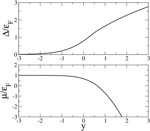
Figure 1: Ultracold fermions in three-dimensions. Upper panel: scaled energy gap $\Delta/\epsilon_{F}$ as a function of scaled interaction strength $y=1/(k_{F}a_{F})$. Lower panel: scaled chemical potential $\mu/\epsilon_{F}$ as a function of scaled interaction strength $y=1/(k_{F}a_{F})$. Note that $k_{F}=(2\pi^{2}n)^{1/3}$ is the Fermi wave number and $\epsilon_{F}=\hbar^{2}k_{F}^{2}/(2m)=(2\pi^{2}n)^{2/3}\hbar^{2}/(2m)$ is the Fermi energy of the 3D ideal three-component Fermi gas with total 3D density $n$.

In the upper panel of Fig. 1 we plot the energy gap $\Delta$ (in units of the Fermi energy $\epsilon_{F}$) as a function of scaled interaction strength $y=1/(k_{F}a_{F})$. As expected the gap $\Delta$ is exponentially small in the BCS region ($y\ll-1$), it becomes of the order of the Fermi energy $\epsilon_{F}$ at unitarity ($y=0$), and then it inceases in the BEC region ($y\gg 1$). In the lower panel of Fig. 1 we show instead the scaled chemical potential $\mu/\epsilon_{F}$ as a function of scaled interaction strength $y=1/(k_{F}a_{F})$. In the BCS region ($y\ll-1$) the chemical potential $\mu$ is positive and practically equal to the Fermi energy $\epsilon_{F}$ of the ideal gas; at unitarity ($y=0$) the $\mu$ is still positive but close to zero; it becomes equal to zero at $y\simeq 0.6$ and then diminishes as $-y^{2}$ (half the binding energy of the formed dimers).

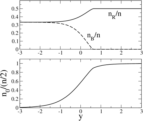
Figure 2: Ultracold fermions in three-dimensions. Upper panel: fraction of red fermions $n_{R}/n$ (solid line) and fraction of blue fermions $n_{B}/n$ (dashed line) as a function of scaled interaction strength $y=1/(k_{F}a_{F})$. Lower panel: condensed fraction of red-green particles $n_{0}/n$ as a function of scaled interaction strength $y=1/(k_{F}a_{F})$. Units as in Fig. 1.

In the upper panel of Fig. 2 we plot the fraction of red fermions $n_{R}/n$ (solid line) and the fraction of blue fermions $n_{B}/n$ (dashed line) as a function of scaled interaction strength $y=1/(k_{F}a_{F})$. The behavior of $n_{G}/n$ is not shown because it is exactly the same of $n_{R}/n$. The figure shows that in the deep BCS regime ($y\ll-1$) the system has $n_{R}/n=n_{G}/n=n_{B}/n=1/3$. By increasing $y$ the fraction of red and green fermions increases while the fraction of blue fermions decreases. At $y\simeq 0.6$, where $\mu=0$, the fraction of blue fermions becomes zero, i.e. $n_{B}/n=0$ and consequently $n_{R}/n=n_{G}/n=1/2$. For larger values of $y$ there are only the paired red and green particles. This behavior is fully consistent with the findings of Ozawa and Baym baym . In the lower panel of Fig.1 it is shown the plot of the condensate fraction $n_{0}/(n/2)$ of red-green pairs through the BCS-BEC crossover as a function of the Fermi-gas parameter $y=1/(k_{F}a_{F})$. The figure shows that a large condensate fraction builds up in the BCS side already before the unitarity limit ($y=0$), and that on the BEC side ($y\gg 1)$ it rapidly converges to one.

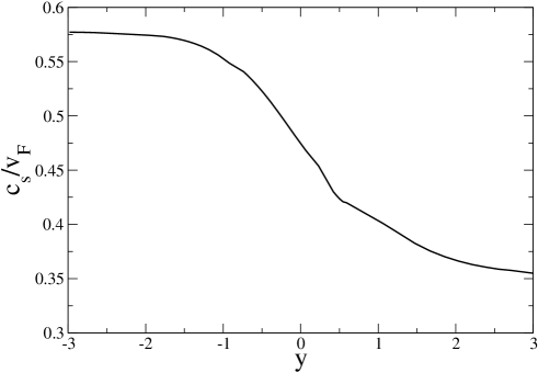
Figure 3: Ultracold fermions in three-dimensions. Scaled sound velocity $c_{s}/v_{F}$ as a function of scaled interaction strength $y=1/(k_{F}a_{F})$. Units as in Fig. 1, with $v_{F}=\hbar k_{F}/m$ the Fermi velocity of the 3D ideal three-component Fermi gas.

As previously stressed, by using Eq. (20) one can obtain the first sound velocity. In particular, we have found that $\mu=\epsilon_{F}\ F(y)$, where $F(y)$ is the numerical function plotted in the lower panel of Fig. 1. It is then straightforward to show that

$$c_{s}={v_{F}\over\sqrt{3}}\sqrt{F(y)-{1\over 2}yF^{\prime}(y)}\;.$$ (37)

By using this formula we plot in Fig. 3 the scaled sound velocity $c_{s}/v_{F}$ as a function of scaled interaction strength $y=1/(k_{F}a_{F})$. The curve shows that $c_{s}/v_{F}$ decreases by increasing $y$ and it shows a knee at $y\simeq 0.6$, where the chemical potential changes sign.

IV Two dimensional case

A two-dimensional Fermi gas can be obtained by imposing a very strong confinement along one of the three spatial directions. In practice, the potential energy $E_{p}$ of this strong external confinement must be much larger than the total chemical potential $\mu_{3D}$ of the fermionic system: $\mu_{3D}\ll 2E_{P}$ io-me . Contrary to the three-dimensional case, in two dimensions quite generally a bound-state energy $\epsilon_{B}$ exists for any value of the interaction strength $g$ between atoms randeria ; marini . For the contact potential the bound-state equation is

$$-{1\over g}={1\over V}\sum_{\bf k}\frac{1}{{\hbar^{2}k^{2}\over 2m}+\epsilon_{B}}\,,$$ (38)

and then subtracting this equation from the gap equation (18) one obtains the two-dimensional regularized gap equation randeria ; marini

$$\sum_{\bf k}\left(\frac{1}{{\hbar^{2}k^{2}\over 2m}+\epsilon_{B}}-{1\over 2E_{k}}\right)=0\;.$$ (39)

Note that, for a 2D inter-atomic potential described by a 2D circularly symmetric well of radius $R_{0}$ and depth $U_{0}$, the bound-state energy $\epsilon_{B}$ is given by $\epsilon_{B}\simeq\hbar^{2}/(2mR_{0}^{2})\exp{(-2\hbar^{2}/(mU_{0}R_{0}^{2}))}$ with $U_{0}R_{0}^{2}\to 0$ landau .

In the two-dimensional continuum limit $\sum_{\bf k}\to V/(2\pi)^{2}\int d^{2}{\bf k}\to V/(2\pi)\int kdk$, the Eq. (39) gives

$$\epsilon_{B}=\Delta\left(\sqrt{1+{\mu^{2}\over\Delta^{2}}}-{\mu\over\Delta}\right)\;.$$ (40)

Note that here $V$ is the 2D volume of the gas, i.e. an area. Instead, the number equation (15) with (16) and (17) gives the total number density as

$$n={N\over V}=n_{R}+n_{G}+n_{B}\;,$$ (41)

where $V$ is a two-dimensional volume (i.e. an area), the red and green densities are

$$n_{R}=n_{G}={1\over 2}\big{(}{m\over 2\pi\hbar^{2}}\big{)}\Delta\left({\mu\over\Delta}+\sqrt{1+{\mu^{2}\over\Delta^{2}}}\right)\;,$$ (42)

while the blue density reads

$$n_{B}=\big{(}{m\over 2\pi\hbar^{2}}\big{)}\mu\ \Theta(\mu)\;.$$ (43)

Finally, the condensate density of red-green pairs is given by

$$n_{0}={1\over 4}\big{(}{m\over 2\pi\hbar^{2}}\big{)}\Delta\left({\pi\over 2}+\arctan{({\mu\over\Delta})}\right)\;.$$ (44)

Also in this two-dimensional case all the relevant quantities can be expressed in terms of the ratio $x_{0}={\mu/\Delta}$, where $x_{0}\in]-\infty,\infty[$. In particular, the scaled pairing gap is given by

$${\Delta\over\epsilon_{F}}={3\over x_{0}+\sqrt{1+x_{0}^{2}}+x_{0}\Theta(x_{0})}\;,$$ (45)

while the scaled chemical potential reads

$${\mu\over\epsilon_{F}}={3x_{0}\over x_{0}+\sqrt{1+x_{0}^{2}}+x_{0}\Theta(x_{0})}\;,$$ (46)

where the two-dimensional Fermi energy $\epsilon_{F}=\hbar^{2}k_{F}^{2}/(2m)$ of the 2D ideal three-component Fermi gas with 2D total density $n$ is given by $\epsilon_{F}=\pi\hbar^{2}n/m$ with $k_{F}=(4\pi n/3)^{1/2}$ the Fermi wave number.

The fraction of red fermions, which is equal to the fraction of green fermions, is given by

$${n_{R}\over n}={n_{G}\over n}={x_{0}+\sqrt{1+x_{0}^{2}}\over 2[x_{0}+\sqrt{1+x_{0}^{2}}+x_{0}\ \Theta(x_{0})]}\;,$$ (47)

the fraction of blue fermions is

$${n_{B}\over n}=1-2{n_{R}\over n}\;,$$ (48)

and the condensate fraction is

$${n_{0}\over n}={{\pi\over 2}+\arctan{(x_{0})}\over 4[x_{0}+\sqrt{1+x_{0}^{2}}+x_{0}\ \Theta(x_{0})]}\;.$$ (49)

It is convenient to express the bound-state energy $\epsilon_{B}$ in terms of the Fermi energy $\epsilon_{F}$. In this way we find

$${\epsilon_{B}\over\epsilon_{F}}=3{\sqrt{1+x_{0}^{2}}-x_{0}\over x_{0}+\sqrt{1+x_{0}^{2}}+x_{0}\ \Theta(x_{0})}\;,$$ (50)

We can now use these parametric formulas of $x_{0}$ to plot the fractions as a function of the scaled bound-state energy $\epsilon_{B}/\epsilon_{F}$.

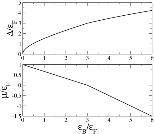
Figure 4: Ultracold fermions in two-dimensions. Upper panel: scaled energy gap $\Delta/\epsilon_{F}$ as a function of scaled bound-state energy $\epsilon_{B}/\epsilon_{F}$. Lower panel: scaled chemical potential $\mu/\epsilon_{F}$ as a function of scaled bound-state energy $\epsilon_{B}/\epsilon_{F}$. Note that $k_{F}=(4\pi n/3)^{1/2}$ is the Fermi wave number and $\epsilon_{F}=\hbar^{2}k_{F}^{2}/(2m)=(4\pi n/3)\hbar^{2}/(2m)$ is the Fermi energy of the 2D ideal three-component Fermi gas with total 2D density $n$.

In the upper panel of Fig. 4 we plot the scaled energy gap $\Delta/\epsilon_{F}$ as a function of scaled binding energy $\epsilon_{B}/\epsilon_{F}$. The gap $\Delta$ is extremely small in the “BCS region” ($\epsilon_{B}/\epsilon_{F}\ll 1/2$), it becomes of the order of the Fermi energy $\epsilon_{F}$ at $\epsilon_{B}/\epsilon_{F}=1/2$, and then it inceases in the “BEC region” ($\epsilon_{B}/\epsilon_{F}\gg 1/2$). In the lower panel of Fig. 4 we show instead the scaled chemical potential $\mu/\epsilon_{F}$ as a function of scaled binding energy $\epsilon_{B}/\epsilon_{F}$. In the BCS region ($\epsilon_{B}/\epsilon_{F}\ll 1/2$) the chemical potential $\mu$ is positive and decreases as $\mu=\epsilon_{F}-\epsilon_{B}/3$; $\mu$ becomes equal to zero at $\epsilon_{B}/\epsilon_{F}=3$ and then it further decreases linearly as $\mu=(3\epsilon_{F}-\epsilon_{B})/2$.

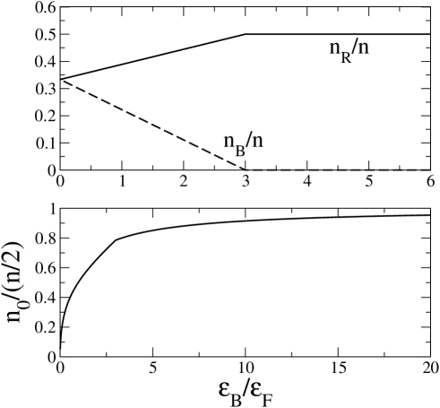
Figure 5: Ultracold fermions in two-dimensions. Upper panel: fraction of red fermions $n_{R}/n$ (solid line) and fraction of blue fermions $n_{B}/n$ (dashed line) as a function of scaled bound-state energy $\epsilon_{B}/\epsilon_{F}$. Lower panel: condensed fraction of red-green particles $n_{0}/n$ as a function of scaled bound-state energy $\epsilon_{B}/\epsilon_{F}$. Units as in Fig. 4.

In the upper panel of Fig. 5 we plot the fraction of red fermions $n_{R}/n$ (solid line) and the fraction of blue fermions $n_{B}/n$ (dashed line) as a function of scaled bound-state energy $\epsilon_{B}/\epsilon_{F}$. The behavior of $n_{G}/n$ is not shown because it is exactly the same of $n_{R}/n$. The figure shows that in the deep BCS regime ($\epsilon_{B}/\epsilon_{F}\ll 1$) the system has $n_{R}/n=n_{G}/n=N_{B}/n=1/3$. By increasing $\epsilon_{B}/\epsilon_{F}$ the fraction of red and green fermions increases while the fraction of blue fermions decreases. At $\epsilon_{B}/\epsilon_{F}=3$, where $\mu=0$, the fraction of blue fermions becomes zero. For larger values of $\epsilon_{B}/\epsilon_{F}$ there are only the paired red and green particles. This behavior is quite similar to the one of the three-dimensional case; the main difference is due to the fact that here the curves are linear. In the lower panel of Fig.5 it is shown the condensate fraction $n_{0}/(n/2)$ of red-green pairs. In the weakly-bound BCS regime ($\epsilon_{B}/\epsilon_{F}\ll 1$) the condensed fraction $n_{0}/n$ goes to zero, while in the strongly-bound BEC regime ($\epsilon_{B}/\epsilon_{F}\gg 1$) the condensed fraction $n_{0}/n$ goes to $1/2$, i.e. all the red-green Fermi pairs belong to the Bose-Einstein condensate. Notice that the condensate fraction is zero when the bound-state energy $\epsilon_{B}$ is zero. For small values of $\epsilon_{B}/\epsilon_{F}$ the condensed fraction has a very fast grow but then it reaches the asymptotic value $1/2$ very slowly.

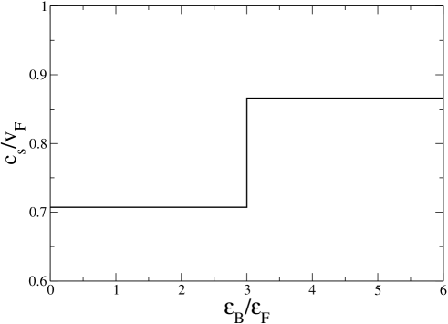
Figure 6: Ultracold fermions in two-dimensions. Scaled sound velocity $c_{s}/v_{F}$ as a function of scaled bound-state energy $\epsilon_{B}/\epsilon_{F}$. Units as in Fig. 4, with $v_{F}=\hbar k_{F}/m$ the Fermi velocity of the 2D ideal three-component Fermi gas.

Also in 2D, by using Eq. (20) one can obtain the first sound velocity. We have found that $\mu=\epsilon_{F}\ G(\epsilon_{B}/\epsilon_{F})$, where $G(\epsilon_{B}/\epsilon_{F})$ is the numerical function plotted in the lower panel of Fig. 4. It is then straightforward to show that

$$c_{s}={v_{F}\over\sqrt{2}}\sqrt{G({\epsilon_{B}\over\epsilon_{F}})-{\epsilon_{B}\over\epsilon_{F}}G^{\prime}({\epsilon_{B}\over\epsilon_{F}})}\;.$$ (51)

By using this formula we plot in Fig. 6 the scaled sound velocity $c_{s}/v_{F}$ as a function of scaled binding energy $\epsilon_{B}/\epsilon_{F}$. The curve shows that $c_{s}/v_{F}$ is constant, i.e. $c_{s}/v_{F}=1/\sqrt{2}$, by increasing $\epsilon_{B}/\epsilon_{F}$ up to $\epsilon_{B}/\epsilon_{F}=3$ where the chemical potential becomes equal to zero. For a larger value of $\epsilon_{B}/\epsilon_{F}$ the sound velocity $c_{s}$ jumps to a larger constant value, i.e. $c_{s}/v_{F}=\sqrt{3}/2$. This kink in the first sound velocity $c_{s}$ is reminescent of the jumps seen with repulsive fermions with reduced dimensionalities io-me ; flavio and with dipolar interaction das .

V Conclusions

We have investigated a uniform three-component ultracold fermions by increasing the SU(3) invariant attractive interaction. We have considered the symmetry breaking of the SU(3) symmetry due to the formation of Cooper pairs both in the three-dimensional case and in the two-dimensional one. We have obtained explicit formulas and plots for energy gap, chemical potential, number densities, condensate density, population imbalance and first sound velocity in the full BCS-BEC crossover. In our calculations we have used the zero-temperature mean-field extended BCS theory, which is expected to give reliable results apart in the deep BEC regime astrakharchik ; ohashi1 ; ohashi2 . Our results are of interest for next future experiments with degenerate gases made of alkali-metal or alkaline-earth atoms. As stressed in the introduction, SU(N) invariant interactions can be experimentaly obtained by using these atomic species selim ; hara ; ana . The problem of unequal couplings, and also that of a fixed number of atoms for each component, is clearly of big interest too, and its analysis can be afforded by including more than one order parameter torma .

There are other interesting open problems about superfluid ultracold atoms we want to face in the next future. In particular, we plan to investigate quasi one-dimensional and quasi two-dimensional Bose-Einstein condensates in nonlinear lattices (i.e. with space-dependent interaction strength) boris-nl . Moreover, we want to analyze the signatures of classical and quantum chaos sala-chaos1 ; sala-chaos2 ; sala-chaos2bis ; sala-chaos3 ; sala-chaos4 with Bose-Einstein condensates in single-well and double-well configurations, and also in the presence of vortices sala-chaos5 ; sala-chaos6 ; sala-chaos7 . Finally, we aim to calculate analytically the coupling tunneling energy of bosons by means of the WKB semiclassical quantization sala-wkb1 ; sala-wkb2 ; sala-wkb3 ; sala-wkb4 and comparing it with the numerical results of the Gross-Pitaevskii equation.

The author thanks Luca Dell’Anna, Giovanni Mazzarella, Nicola Manini, Carlos Sa de Melo, Flavio Toigo and Andrea Trombettoni for useful discussions and suggestions.

References

- (1) A.J. Leggett, Quantum Liquids: Bose Condensation and Cooper Pairing in Condensed-Matter Systems (Oxford Univ. Press, Oxford, 2006).
- (2) H.T.C. Stoof, B.M. Dennis, and K. Gubbels, Ultracold Quantum Fields (Springer, Berlin, 2009).
- (3) G. Diana, N. Manini, and L. Salasnich, Phys. Rev. A 73 065601 (2006).
- (4) L. Salasnich and N. Manini, Laser Phys. 17, 169 (2007).
- (5) L. Salasnich, F. Ancilotto, and F. Toigo, Laser Phys. Lett. 7, 78 (2010).
- (6) Y. Cheng and S.K. Adhikari, Laser Phys. Lett. 7, 824 (2010).
- (7) Y.I. Yukalov, Laser Phys. Lett. 7, 467 (2010).
- (8) R.F. Shiozaki, G.D. Telles, Y.I. Yukalov, and V.S. Bagnato, Laser Phys. Lett. 8, 393 (2011).
- (9) T.B. Ottenstein, T. Lompe, M. Kohen, A.N. Wenz, and S. Jochim, Phys. Rev. Lett. 101, 203202 (2008).
- (10) J.H. Huckans, J.R. Williams, E.L. Hazlett, R.W. Stites, and K. M. O’Hara, Phys. Rev. Lett. 102, 165302 (2009).
- (11) C. Wu, J.P. Hu, and S.C. Zhang, Phys. Rev. Lett. 91, 186402 (2003).
- (12) C. Wu, Mod. Phys. Lett. B 20, 1707 (2006).
- (13) A.V. Gorshkov, M. Hermele, V. Gurarie, C. Xu, P.S. Julienne, J. Ye, P. Zoller, E. Demler, M.D. Lukin, A.M. Rey, Nature Physics 6, 289 (2010).
- (14) A.G.K. Modawi and A.J. Leggett, J. Low Temp. Phys. 109, 625 (1997).
- (15) C. Honerkamp and W. Hofstetter, Phys. Rev. Lett. 92, 17040 (2004).
- (16) T. Paananen, J.-P. Martikainen, and P. Torma, Phys. Rev. A 73, 053606 (2006).
- (17) C.K. Chung and C.K. Law, Phys. Rev. A 82, 033620 (2010).
- (18) L. He, M Jin, and P. Zhang, Phys. Rev. A 74, 033604 (2006).
- (19) T. Ozawa and G. Baym, Phys. Rev. A 82, 063615 (2010).
- (20) D.M. Eagles, Phys. Rev. 186, 456 (1969).
- (21) A.J. Leggett, in Modern Trends in the Theory of Condensed Matter, p. 13, edited by A. Pekalski and J. Przystawa (Springer, Berlin, 1980).
- (22) M. Randeria, J.-M. Duan, and L.-Y. Sheih, Phys. Rev. B 41, 327 (1990).
- (23) M. Marini, F. Pistolesi, and G.C. Strinati, Eur. Phys. J. B 1, 151 (1998).
- (24) M.Y. Kagan and S.L. Ogarkov, Laser Phys. 18, 509 (2008).
- (25) L. Salasnich, Phys. Rev. A 83, 033630 (2011).
- (26) M.W. Zwierlein, C.A. Stan, C.H. Schunck, S.M.F. Raupach, A.J. Kerman, and W. Ketterle, Phys. Rev. Lett. 92, 120403 (2004).
- (27) M.W. Zwierlein, C.H. Schunck, C.A. Stan, S.M.F. Raupach, and W. Ketterle, Phys. Rev. Lett. 94, 180401 (2005).
- (28) Y. Inada, M. Horikoshi, S. Nakajima, M. Kuwata-Gonokami, M. Ueda, and T. Makaiyama, Phys. Rev. Lett. 101, 180406 (2008).
- (29) L. Salasnich, N. Manini, and A. Parola, Phys. Rev. A 72, 023621 (2005).
- (30) G. Ortiz and J. Dukelsky, Phys. Rev. A 72, 043611 (2005).
- (31) G. E. Astrakharchik, J. Boronat, J. Casulleras, and S. Giorgini, Phys. Rev. Lett. 95, 230405 (2005).
- (32) Y. Ohashi and A. Griffin, Phys. Rev. A 72, 063606 (2005).
- (33) N. Fukushima, Y. Ohashi, E. Taylor, and A. Griffin, Phys. Rev. A 75, 033609 (2007).
- (34) L. Salasnich, Phys. Rev. A 76, 015601 (2007).
- (35) L.D. Landau and E.M. Lifshits, Statistical Physics, Part 2, vol. 9 (Butterworth-Heinemann, Oxford, 1980).
- (36) L.D. Landau and E.M. Lifshitz, Quantum Mechanics. Non Relativistic Theory. Course of Theoretical Physics, Vol. 3 (Pergamon Press, New York, 1989).
- (37) G. Mazzarella, L. Salasnich, and F. Toigo, Phys. Rev. A 79, 023615 (2009).
- (38) L. Salasnich, and F. Toigo, J. Low Temp. Phys. 150, 643 (2008).
- (39) J.P. Kestner and S. Das Sarma, Phys. Rev. A 82, 033608 (2010).
- (40) O.H.T. Nummi, J.J. Kinnunen, and P. Torma, New J. Phys. 13, 055013 (2011).
- (41) Y.V. Kartashov, B.A. Malomed, and L. Torner, Rev. Mod. Phys. 83, 247 (2011).
- (42) L. Salasnich, Phys. Rev. D 52, 6189 (1995).
- (43) L. Salasnich, Mod. Phys. Lett. A 12, 1473 (1997).
- (44) L. Salasnich, Phys. Lett. A 266, 187 (2000).
- (45) A.R. Kolovsky and A. Buchleitner, Europhys. Lett. 68 632 (2004).
- (46) C. Weiss and N. Teichmann, Phys. Rev. Lett. 100, 140408 (2008).
- (47) L. Salasnich, Int. J. Mod. Phys. B 14, 1 (2000).
- (48) L. Salasnich, Laser Phys. 14, 291 (2004).
- (49) S.K. Adhikari and L. Salasnich, Phys. Rev. A 75, 053603 (2007).
- (50) M. Robnik and L. Salasnich, J. Phys. A: Math. Gen. 30, 1711 (1997).
- (51) M. Robnik and L. Salasnich, J. Phys. A: Math. Gen. 30, 1719 (1997).
- (52) G. Alvarez, J. Math. Phys. 45, 3095 (2004).
- (53) A.V. Turbiner, Int. J. Mod. Phys. A 25, 647 (2010).