From homogenization to averaging in cellular flows

Abstract

We consider an elliptic eigenvalue problem with a fast cellular flow of amplitude $A$, in a two-dimensional domain with $L^{2}$ cells. For fixed $A$, and $L\to\infty$, the problem homogenizes, and has been well studied. Also well studied is the limit when $L$ is fixed, and $A\to\infty$. In this case the solution equilibrates along stream lines.

In this paper, we show that if both $A\to\infty$ and $L\to\infty$, then a transition between the homogenization and averaging regimes occurs at $A\approx L^{4}$. When $A\gg L^{4}$, the principal Dirichlet eigenvalue is approximately constant. On the other hand, when $A\ll L^{4}$, the principal eigenvalue behaves like ${\bar{\sigma}(A)}/L^{2}$, where $\bar{\sigma}(A)\approx\sqrt{A}I$ is the effective diffusion matrix. A similar transition is observed for the solution of the exit time problem. The proof in the homogenization regime involves bounds on the second correctors. Miraculously, if the slow profile is quadratic, these estimates can be obtained using drift independent $L^{p}\to L^{\infty}$ estimates for elliptic equations with an incompressible drift. This provides effective sub and super-solutions for our problem.

1 Introduction

Consider an advection diffusion equation of the form

$$\partial_{t}\varphi+Av(x)\cdot\nabla\varphi-\Delta\varphi=0.$$ (1.1)

where $A$ is the non-dimensional strength of a prescribed vector field $v(x)$. Under reasonable assumptions when $A\to\infty$, the solution $\varphi$ becomes constant on the trajectories of $v$. Indeed, dividing (1.1) by $A$ and passing to the limit $A\to\infty$ formally shows

$$v(x)\cdot\nabla\varphi=0,$$

which, of course, forces $\varphi$ to be constant along trajectories of $v$. Well known “averaging” results [FW, Kifer, PS] study the slow evolution of $\varphi(t,x)$ across various trajectories.

On the other hand, if we fix $A=1$, classical homogenization results [BLP, KOZ, PS] determine the long time behavior of solutions of (1.1). For such results it is usually convenient to choose $\varepsilon\ll 1$ small, and rescale (1.1) to time scales of order $1/\varepsilon^{2}$, and distance scales of order $1/\varepsilon$. This gives

$$\partial_{t}\varphi_{\varepsilon}+\frac{1}{\varepsilon}v\left(\frac{x}{\varepsilon}\right)\cdot\nabla\varphi_{\varepsilon}-\Delta\varphi_{\varepsilon}=0.$$ (1.2)

Assuming $v$ is periodic, and that the initial condition varies slowly (i.e. $\varphi_{\varepsilon}(x,0)$ is independent of $\varepsilon$), standard homogenization results show that $\varphi_{\varepsilon}\to\bar{\varphi}$, as $\varepsilon\to 0$. Further, $\bar{\varphi}$ is the solution of the effective problem

$$\frac{\partial\bar{\varphi}}{\partial t}=\nabla\cdot(\bar{\sigma}\nabla\varphi),$$ (1.3)

and $\bar{\sigma}$ is the effective diffusion matrix, which can be computed as follows. Define the correctors $\chi_{1}$, …, $\chi_{n}$ to be the mean-zero periodic solutions of

$$-\Delta\chi_{j}+v(x)\cdot\nabla\chi_{j}=-v_{j}(x),\quad j=1,\dots,n.$$ (1.4)

Then

$$\bar{\sigma}_{ij}=\delta_{ij}+\frac{1}{\lvert Q\rvert}\int_{Q}\nabla\chi_{i}\cdot\nabla\chi_{j}\,dx,\quad i,j=1,\dots,n.$$ (1.5)

$Q$ is the period cell of the flow $v(x)$, and $\delta_{ij}$ is the Kronecker delta function.

The main focus of this paper is to study a transition between the two well known regimes described above. To this end, rescale (1.1) by choosing time scales of the order $1/\varepsilon^{2}$ and length scales of order $1/\varepsilon$. This gives

$$\partial_{t}\varphi_{\varepsilon,A}+\frac{A}{\varepsilon}v\left(\frac{x}{\varepsilon}\right)\cdot\nabla\varphi_{\varepsilon,A}-\Delta\varphi_{\varepsilon,A}=0,$$ (1.6)

where $A\gg 1$ and $\varepsilon\ll 1$ are two independent parameters. Of course, if we keep $\varepsilon$ fixed, and send $A\to\infty$, the well known averaging results apply. Alternately, if we keep $A$ fixed and send $\varepsilon\to 0$, we are in the regime of standard homogenization results. The present paper considers (1.6) with both $\varepsilon\to 0$ and $A\to\infty$. Our main result shows that if $v$ is a $2D$ cellular flow, then we see a sharp transition between the homogenization and averaging regimes at $A\approx 1/\varepsilon^{4}$.

Before stating our precise results (Theorems 1.1 and 1.2 below), we provide a brief explanation as to why one expects the transition to occur at $A\approx 1/\varepsilon^{4}$. For simplicity and concreteness, we choose the stream function $H(x_{1},x_{2})=\frac{1}{\pi}\sin(\pi x_{1})\sin(\pi x_{2})$, and define $v(x_{1},x_{2})=(-\partial_{2}H,\partial_{1}H)$. Even in this simple setting, to the best of our knowledge, the transition from averaging to homogenization has not been studied before.

First, for any fixed $A$, we let $\bar{\sigma}(A)=(\bar{\sigma}_{ij}(A))$ denote the effective diffusion matrix obtained in the limit $\varepsilon\to 0$ (see [KramerMajda] for a comprehensive review). If $\chi_{j}^{A}$ is the mean zero, $2$-periodic solution to

$$-\Delta\chi_{j}^{A}+Av(x)\cdot\nabla\chi_{j}=-Av_{j}(x),\quad\text{for }j\in\{1,2\},$$ (1.7)

then the effective diffusivity (as a function of $A$) is given by (1.5). As $A\to\infty$, the behaviour of the correctors $\chi_{j}^{A}$ is well understood [bblChildress, bblFannjiangPapanicolaou, Heinze, Koralov, bblNovikovPapanicolaouRyzhik, bblRosenbluth, bblShraiman, bblYoung]. Except on a boundary layer of order $1/\sqrt{A}$, each of the functions $\chi_{j}(x)+x_{j}$ become constant in cell interiors. Using this one can show (see for instance [bblChildress, bblFannjiangPapanicolaou]) that asymptotically, as $A\to\infty$, the effective diffusion matrix behaves like

$$\bar{\sigma}(A)=\sigma_{0}\sqrt{A}I+o(\sqrt{A})$$ (1.8)

Here $I$ is the identity matrix, and $\sigma_{0}>0$ is an explicitly computable constant. Consequently, if we consider (1.6), with the Dirichlet boundary conditions on the unit square, we expect

$$\varphi_{\varepsilon,A}(x,t)\approx\exp(-\sigma_{0}\sqrt{A}t),\quad\text{as $t\to\infty$, for small $\varepsilon$.}$$ (1.9)

On the other hand, if we keep $\varepsilon$ fixed and send $A\to\infty$, we know [FW, bblYoung] that $\varphi$ becomes constant on stream lines of $H$. In particular, because of the Dirichlet boundary condition on the outside boundary, we must also have $\varphi=0$ on the boundary of all interior cells. Since these cells have side length $\varepsilon$, we expect

$$\varphi_{\varepsilon,A}(x,t)\approx\exp(-\pi^{2}t/\varepsilon^{2}),\quad\text{as $t\to\infty$ for large $A$.}$$ (1.10)

Matching (1.9) and (1.10) leads us to believe $\sqrt{A}\approx 1/\varepsilon^{2}$ marks the transition between the two regimes.

With this explanation, we state our main results. Our first two results study the averaging to homogenization transition for the principal Dirichlet eigenvalue. Let $L$ be an even integer, $D=[-L/2,L/2]\times[-L/2,L/2]$ be a square of side length $L$, and $A>0$ be given. We study the principal eigenvalue problem on $D$

$$\left\{\begin{aligned} -\Delta\varphi+Av\cdot\nabla\varphi&=\lambda\varphi&&\text{in }D\\ \varphi&=0&&\text{on }\partial D\\ \varphi&>0&&\text{in }D,\end{aligned}\right.$$ (1.11)

as both $L,A\to\infty$. We observe two distinct behaviors of $\lambda$ with a sharp transition. If $A\gg L^{4}$, then the principal eigenvalue stays bounded, and can be read off using the variational principle in [bblBeresHamelNadirshvilli] in the limit $A\to\infty$. This is the averaging regime, and exactly explains (1.10). On the other hand, if $A\ll L^{4}$, then the principal eigenvalue is of the order ${\bar{\sigma}(A)}/{L^{2}}$. This is the homogenization regime, and when rescaled to a domain of size $1$, exactly explains (1.9). Our precise results are stated below.

Theorem 1.1 (The averaging regime).

Let $\varphi=\varphi_{L,A}$ be the solution of (1.11) and $\lambda=\lambda_{L,A}$ be the principal eigenvalue. If $A\to\infty$, and $L=L(A)$ varies such that

$$\liminf_{A\to\infty}\frac{\sqrt{A}}{L^{2}\log A\log L}>0,$$ (1.12)

then there exist two constants $\lambda_{0},\lambda_{1}$, independent of $L$ and $A$, such that

$$0<\lambda_{0}\leqslant\lambda_{L,A}\leqslant\lambda_{1}<\infty$$ (1.13)

for all $A$ sufficiently large.

Theorem 1.2 (The homogenization regime).

As with Theorem 1.1, let $\varphi=\varphi_{L,A}$ be the solution of (1.11) and $\lambda=\lambda_{L,A}$ be the principal eigenvalue. If $L\to\infty$, and $A=A(L)$ varies such that

$$\frac{1}{c}L^{4-\alpha}\leqslant A\leqslant cL^{4-\alpha},\quad\text{for some }\alpha>0,$$ (1.14)

then there exists a constant $C=C(\alpha,c)>0$, independent of $L$ and $A$, such that

$$\frac{1}{C}\frac{\sqrt{A}}{L^{2}}\leqslant\lambda_{L,A}\leqslant C\frac{\sqrt{A}}{L^{2}}$$ (1.15)

for all $L$ sufficiently large.

Remark.

In the special case where $A=L^{\beta}$, for $\beta>4$, assumption (1.12) is satisfied, and consequently the principal eigenvalue remains bounded and non-zero. For $\beta<4$, assumption (1.14) is satisfied and the principal eigenvalue behaves like that of the homogenized equation.

In the averaging regime (Theorem 1.1), the proof of the upper bound in (1.13) follows directly using ideas of [bblBeresHamelNadirshvilli]. The lower bound, however, is much more intricate. The main idea is to control the oscillation of $\varphi$ between neighbouring cells, and use this to show that the effect of the cold boundary propagates inward along separatrices, all the way to the center cell. The techniques used are similar to [bblFannjiangKiselevRyzhik, bblKiselevRyzhik]. The main new (and non-trivial) difficulty in our situation is that the number of cells also increases with the amplitude. This requires us to estimate the oscillation of $\varphi$ between cells in terms of energies localised to each cell (Proposition 2.4, below). Here the assumption that $L$ is not too large comes into play. Finally, the key idea in the proof is to use a min-max argument (Lemma 2.5, below) to show that $\varphi$ is small on the boundaries of all cells.

Moreover, once smallness on separatrices is established, our proof may be modified to show that under a stronger assumption

$$\liminf_{A\to\infty}\frac{\sqrt{A}}{L^{2}\log A\log L}=+\infty,$$ (1.16)

we have a precise asymptotics

$$\lim_{A\to\infty}\lambda_{L,A}=\inf\left\{\int_{Q}\lvert\nabla w\rvert^{2}\;\middle|\;w\in H^{1}_{0}(Q),\int_{Q}w^{2}=1,\text{ and }w\cdot\nabla v=0\right\},$$ (1.17)

where $Q$ is a single cell. This is the same as the variational principle in [bblBeresHamelNadirshvilli]. We remark however that [bblBeresHamelNadirshvilli] only gives (1.17) for fixed $L$ as $A\to\infty$.

Turning to the homogenization regime (Theorem 1.2), we remark first that homogenization of eigenvalues has not been as extensively studied as other homogenization problems. This is possibly because eigenvalues involve the infinite time horizon. We refer to [AlCap, Kes1, Kes2, SV1, SV2] that all study self-adjoint problems for some results on the homogenization of the eigenvalues in oscillatory periodic media. The extra difficulties in the present paper come both from two sources. First, since the problem is not self adjoint, a variational principle for the eigenvalue is not available. Second, as $A$ and $L$ tend to $\infty$, we don’t have suitable aprori bounds because either the domain is not compact, or the effective diffusivity is unbounded.

Our proof uses a multi-scale expansion to construct appropriate sub and super solutions. When $A$ is fixed, it usually suffices to consider a multi-scale expansion to the first corrector. However, in our situation, this is not enough, and we are forced to consider a multi-scale expansion up to the second corrector.

Of course an asymptotic profile, and explicit bounds are readily available [bblFannjiangPapanicolaou] for the first corrector. However, to the best of our knowledge, bounds on the second corrector as $A\to\infty$ have not been studied. There are two main problems to obtaining these bounds. The first problem is appearance of that terms involving the slow gradient of the second corrector multiplied by $A$. In general, we have no way of bounding these terms. Luckily, if we choose our slow profile to be quadratic, then these terms idnetically vanish and present no problem at all!

The second problem with obtaining bounds on the second corrector is that it satisfies an equation where the first order terms depend on $A$. So one would expect the bounds to also depend on $A$, which would be catastrophic in our situation. However, for elliptic equations with a divergence free drift, we have apriori $L^{p}\to L^{\infty}$ estimates which are independent of the drift [bblBerestyckiKiselevNovikovRyzhik, bblFannjiangKiselevRyzhik]. This, combined with an explicit knowledge of the first corrector, allows us to obtain bounds on the second corrector that decay when $A\ll L^{4}$.

The sub and super solutions we construct for eigenvalue problem are done through the expected exit time. Since these are interesting in their own right, we describe them below. Let $\tau=\tau_{L,A}$ be the solution of

$$\left\{\begin{gathered}-\Delta\tau+Av\cdot\nabla\tau=1\quad\text{in }D\\ \tau=0\quad\text{on }\partial D,\end{gathered}\right.$$ (1.18)

where $v$ and $D$ are as in (1.11). Though we do not use any probabilistic arguments in this paper, it is useful to point out the connection between $\tau$ and diffusions. Let $X$ be the diffusion

$$dX_{t}=-Av(X_{t})\,dt+\sqrt{2}dW_{t}$$ (1.19)

where $W$ is a standard $2$-dimensional Brownian motion. It is well known that $\tau$ is the expected exit time of the diffusion $X$ from the domain $D$. Numerical simulations of three realizations of $X$ are shown in Figure 1. Note that for “small” amplitude ($A=L^{3}$), trajectories of $X$ behave similarly to those of the Brownian motion. For a “large” amplitude ($A=L^{4.5}$), trajectories of $X$ tend to move ballistically along the skeleton of the separatrices.

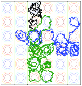
(a) Small amplitude ($A=L^{3}$)

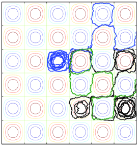
(b) Large amplitude ($A=L^{4.5}$)

Figure 1: Trajectories of three realizations of the diffusion (1.19).

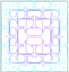
(a) Small amplitude ($A=L^{3}$)

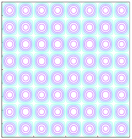
(b) Large amplitude ($A=L^{5}$)

Figure 2: A contour plot of $\tau(x,y)$.

Similar to the eigenvalue problem, the behaviour of $\tau$ is described by two distinct regimes with a sharp transition. If $A\gg L^{4}$, then the stirring is strong enough to force the diffusion $X$ to exit $D$ almost immediately along separatrices. In this case, we show that $\tau\to 0$ on separatrices, and is bounded everywhere else above by a constant independent of $A$ and $L$. On the other hand, if $A\ll L^{4}$, then the stirring is not strong enough for the effect of the cold boundary to be felt in the interior. In this case, it takes the diffusion $X$ a very long time to exit from $D$, and $\tau\to\infty$ as $A,L\to\infty$. A numerical simulation showing $\tau$ in each of these regimes is shown in Figure 2. The precise results are as follows.

Theorem 1.3 (The averaging regime).

Let $\tau=\tau_{L,A}$ be the solution to (1.18). Let $A\to\infty$, and suppose $L=L(A)$ varies such that (1.12) is satisfied. There exists a constant $C$, independent of $A$, $L$, such that for all $A$ sufficiently large

$$\tau(x)^{2}\leqslant C\frac{L^{2}}{\sqrt{A}}\log A\log L,\quad\text{whenever }H(x)=0.$$

Consequently, if $H(x)=0$, then $\tau(x)\to 0$ as $A\to\infty$, and $\lVert\tau\rVert_{L^{\infty}(D)}$ is bounded uniformly in $A$.

Theorem 1.4 (The homogenization regime).

As with Theorem 1.3, let $\tau=\tau_{L,A}$ be the solution of (1.18) on the square $D=[-L/2,L/2]\times[-L/2,L/2]$. Suppose now $L\to\infty$, and $A=A(L)$ varies such that (1.14) is satisfied, for some fixed $\alpha\in(0,4)$. Then, for any $\delta>0$, there exists a constant $C=C(\delta,\alpha,c)>0$, independent of $A$, $L$, such that

$$C^{-1}\frac{L^{2}}{\sqrt{A}}\leqslant\tau(x)\leqslant C\frac{L^{2}}{\sqrt{A}},\quad\text{whenever }\left\lvert x\right\rvert\leqslant(1-\delta)\frac{L}{2}$$ (1.20)

for all $L$ sufficiently large. Consequently, $\tau\to\infty$ as $L\to\infty$, uniformly on compact sets.

The proof of Theorem 1.3 is similar steps to that of Theorem 1.1. For the proof of Theorem 1.4, as mentioned earlier, we need to perform a multi-scale expansion up to two correctors, and choose the slow profile to be quadratic. When the domain is a disk, a quadratic function is exactly the solution to the homogenized problem! This gives us a sharper estimate for $\tau$.

Proposition 1.5.

Let $B_{L}$ be a disk of radius $L$, and $\tau_{A,L}$ be the solution of (1.18) in $B_{L}$. If $A$ and $L$ satisfy the assumptions in Theorem 1.4 then

$$\left\lvert\tau(x)-\frac{1}{2\operatorname{tr}(\bar{\sigma}(A))}\left(L^{2}-\lvert x\rvert^{2}\right)\right\rvert\leqslant c\frac{L}{A^{1/4}}$$ (1.21)

where $c>0$ is independent of $A$ and $L$. Here $\bar{\sigma}(A)$ is the effective diffusion matrix and $\operatorname{tr}(\bar{\sigma}(A))$ denotes the trace of this matrix.

Remark 1.6.

Note that right hand side of(1.21) tends to infinity as $A,L\to\infty$. However, by (1.8) the terms on the left are of order $L^{2}/\sqrt{A}$, which dominates the right hand side. Thus (1.21) immediately implies (1.20).

By fitting a disk inside, and outside a square, Proposition 1.5 quickly implies Theorem 1.4. Further, since it is well known that the principal eigenvalue is bounded below by the maximum expected exit time, the lower bound in Theorem 1.2 also quickly follows from Proposition 1.5. The upper bound is a little more technical, however, also uses Proposition 1.5 as the main idea.

We mention that we have chosen to use the particular form of the stream-function $H(x_{1},x_{2})=\frac{1}{\pi}\sin(\pi x_{1})\sin(\pi x_{2})$ simply for the sake of convenience. All our results may be generalized to other periodic flows with a cellular structure without any difficulty. We also believe that for other flows the transition from the averaging to the homogenization regime happens when the effective diffusivity $\bar{\sigma}(A)$ balances with the domain size $L$. That is, when the “homogenized eigenvalue” $\bar{\sigma}(A)/L^{2}$ is of the same order as the “strong flow” eigenvalue:

$$\lim_{A\to\infty}\frac{\bar{\sigma}(A)}{L^{2}\lambda_{L,A}}\approx 1.$$ (1.22)

We leave this question for a future study.

This paper is organized as follows. The averaging regime is considered in Sections 2 and 3. The former contains the proof of Theorem 1.1 and the latter of Theorem 1.3. The rest of the paper addresses the homogenization regime. The key step here is Proposition 1.5 proved in Section 4. From this, Theorem 1.4 quickly follows, and the proof is presented the same section. Theorem 1.2 is proved in Section 5.

Acknowledgement

GI was supported by NSF grant DMS-1007914, TK by Polish Ministry of Science and Higher Education grant NN 201419139, AN by NSF grant DMS-0908011, and LR by NSF grant DMS-0908507, and NSSEFF fellowship. We thank Po-Shen Loh for suggesting the proof of Lemma 2.5.

2 The eigenvalue in the strong flow regime

In this section we present the proof of Theorem 1.1. First, we discuss the proof of the upper bound in (1.13), followed by the proof of the corresponding lower bound, and, finally, of the limiting behavior in (1.17).

2.1 The upper bound

The upper bound for $\lambda$ in (1.13) follows directly from the techniques of [bblBeresHamelNadirshvilli]. We carry out the details below. Following [bblBeresHamelNadirshvilli], given any test function $w\in H^{1}_{0}(D)$, and a number $\alpha>0$, we multiply (1.11) by ${w^{2}}/{(\varphi+\alpha)}$ and integrate over $D$ to obtain

$$\lambda\int_{D}\frac{w^{2}\varphi}{\varphi+\alpha}=-\int_{D}\frac{w^{2}\Delta\varphi}{\varphi+\alpha}+A\int_{D}\frac{w^{2}}{\varphi+\alpha}v\cdot\nabla\varphi.$$ (2.1)

For the first term on the right, we have

$$-\int_{D}\frac{w^{2}\Delta\varphi}{\varphi+\alpha}=\int_{D}\nabla\varphi\cdot\left(\frac{2w(\varphi+\alpha)\nabla w-w^{2}\nabla\varphi}{(\varphi+\alpha)^{2}}\right)$$

$$=\int_{D}\lvert\nabla w\rvert^{2}-\int_{D}\frac{\lvert w\nabla\varphi-(\varphi+\alpha)\nabla w\rvert^{2}}{(\varphi+\alpha)^{2}}\leqslant\int_{D}\lvert\nabla w\rvert^{2}.$$

For the second term on the right of (2.1) we have, since $u$ is incompressible,

$$\int_{D}\frac{w^{2}}{\varphi+\alpha}v\cdot\nabla\varphi=\int_{D}w^{2}v\cdot\nabla\ln(\varphi+\alpha)=-2\int_{D}\ln(\varphi+\alpha)w(v\cdot\nabla w).$$

Hence, equation (2.1) reduces to

$$\lambda\int_{D}\frac{w^{2}\varphi}{\varphi+\alpha}\leqslant\int_{D}\lvert\nabla w\rvert^{2}-2A\int_{D}\ln(\varphi+\alpha)w(v\cdot\nabla w).$$ (2.2)

Now, choose $w$ to be any $H^{1}_{0}(D)$ first integral of $v$ (that is, $v\cdot\nabla w=0$). Then, equation (2.2) reduces to

$$\lambda\int_{D}\frac{w^{2}\varphi}{\varphi+\alpha}\leqslant\int_{D}\lvert\nabla w\rvert^{2}.$$

Upon sending $\alpha\to 0$, the Monotone Convergence Theorem shows

$$\lambda\int_{D}w^{2}\leqslant\int_{D}\lvert\nabla w\rvert^{2}$$

for any $H^{1}_{0}(D)$ first integral of $v$. Choosing $w=H(x)$, which, of course, does not depend on $L$, we immediately see that

$$\lambda\leqslant\left(\int_{D}H^{2}\right)^{-1}\int_{D}\lvert\nabla H\rvert^{2}=\left(L^{2}\int_{Q_{0}}H^{2}\right)^{-1}L^{2}\int_{Q_{0}}\lvert\nabla H\rvert^{2}\\ =\left(\int_{Q_{0}}H^{2}\right)^{-1}\int_{Q_{0}}\lvert\nabla H\rvert^{2},$$

where $Q_{0}$ is any cell in $D$. This gives a finite upper bound for $\lambda$ that is independent of $L$ and $A$.

2.2 The lower bound

The outline of the proof is as follows. The basic idea is that if the domain size $L$ is not too large, and the flow is sufficiently strong, the eigenfunction $\varphi$ should be small not only near the boundary $\partial D$ but also on the whole skeleton of separatrices inside $D$. Therefore, the Dirichlet eigenvalue problem for the whole domain $D$ is essentially equivalent to a one-cell Dirichlet problem, which gives the correct asymptotics for the eigenvalue for $A$ large. To this end, we first estimate the oscillation of $\varphi$ along a streamline of $v$ inside one cell that is sufficiently close to the separatrix, and show that this oscillation is small: see Lemma 2.2. Next, we show that the difference of the values of $\varphi$ on two streamlines of $v$ (sufficiently close to the separatrix) in two neighbouring cells must be small, as in Lemma 2.3 below. These two steps are very similar to those in [bblFannjiangKiselevRyzhik], and their proofs are only sketched.

Now, considering the ‘worst case scenario’ of the above oscillation estimates, we obtain a pointwise upper bound on $\varphi$ on streamlines of $v$ near separatrices in terms of the principal eigenvalue $\lambda$, and $\lVert\varphi\rVert_{L^{2}}^{2}$: see Lemma 2.5. Next, we show that the streamlines above enclose a large enough region to encompass most of the mass of $\varphi^{2}$. Finally, we use the drift independent apriori estimates in [bblBerestyckiKiselevNovikovRyzhik, bblIyerNovkiovRyzhikZlatos] to obtain the desired lower bound on $\lambda$.

A streamline oscillation estimate

The basic reason behind the fact that the eigenfunction is constant on streamlines is the following estimate, originally due to S. Heinze [Heinze].

Lemma 2.1.

There exists a constant $C>0$ so that we have

$$\int_{D}|v\cdot\nabla\varphi|^{2}dx\leqslant\frac{C}{A}\int_{D}|\nabla\varphi|^{2}dx=\frac{C\lambda}{A}\|\varphi\|_{L^{2}}^{2}.$$ (2.3)

• Let us use the normalization $\|\varphi\|_{L^{2}}=1$. We multiply (1.11) by $v\cdot\nabla\varphi$, and integrate over $Q_{i}$. This gives

  $$A\int_{D}\lvert v\cdot\nabla\varphi\rvert^{2}=\lambda\int_{D}\varphi(v\cdot\nabla\varphi)+\int_{D}\Delta\varphi(v\cdot\nabla\varphi).$$

  Notice that

  $$\int_{D}\varphi(v\cdot\nabla\varphi)=\frac{1}{2}\int_{D}v\cdot\nabla\left(\varphi^{2}\right)=0,$$

  since $v\cdot\nu=0$ on $\partial Q_{i}$ and $\nabla\cdot v=0$. Similarly, we have, as $v\cdot\nabla\varphi=0$ on $\partial D$:

  $$\int_{D}\Delta\varphi(v\cdot\nabla\varphi)=-\sum_{j=1}^{2}\int_{D}\partial_{j}\varphi\left(\partial_{j}v\cdot\nabla\varphi\right)-\sum_{j=1}^{2}\int_{D}\partial_{j}\varphi\left(v\cdot\nabla\partial_{j}\varphi\right)+\int_{\partial D}(\nu\cdot\nabla\varphi)(v\cdot\nabla\varphi)\,dS\\ \leqslant\lVert\nabla v\rVert_{L^{\infty}(Q_{i})}\lVert\nabla\varphi\rVert_{L^{2}(D)}^{2}-\frac{1}{2}\sum_{j=1}^{2}\int_{D}\nabla\cdot\left(v\left(\partial_{j}\varphi\right)^{2}\right)=C\lambda,$$

  and consequently we obtain (2.3). ∎

The next lemma bounds locally the oscillation on streamlines in terms of the $L^{2}$-norm of $v\cdot\nabla\varphi$.

Lemma 2.2.

Let $Q_{i}$ be any cell. For any $\delta_{0}>0$, there exists $\Gamma_{i}\subset Q_{i}$ such that $\Gamma_{i}$ is a level set of $H$, $\lvert H(\Gamma_{i})\rvert\in(\delta_{0},2\delta_{0})$, and

$$\sup_{x_{1},x_{2}\in\Gamma_{i}}\lvert\varphi(x_{1})-\varphi(x_{2})\rvert^{2}\leqslant C\frac{1}{\delta_{0}}\log\left(\frac{1}{\delta_{0}}\right)\int_{Q_{i}}\lvert v\cdot\nabla\varphi\rvert^{2}.$$ (2.4)

for some constant $C$ independent of $A,L,\delta_{0}$.

We will see that $\delta_{0}$ is the ‘width’ of the boundary layer, and will eventually be chosen to be $\delta_{0}\approx{1}/{\sqrt{A}}$.

• The proof is straightforward and similar bounds have already appeared in [bblKiselevRyzhik, bblFannjiangKiselevRyzhik]. We sketch the details here for convenience. First we introduce curvilinear coordinates in the cell $Q_{i}$. For this, let $(x_{i},y_{i})$ be the center of $Q_{i}$, and $\Theta_{i}$ be the solution of

  $$\left\{\begin{aligned} \nabla\Theta_{i}\cdot\nabla H&=0&&\text{in }Q_{i}-\{(x_{i}+t,y_{i})\;|\;t\geqslant 0\}\\ \Theta_{i}(x,y)&=\tan^{-1}\left(\frac{y-y_{i}}{x-x_{i}}\right)&&\text{on }\partial Q_{i}.\end{aligned}\right.$$ (2.5)

  As usual, we extend $\Theta$ to $Q_{i}$ by defining it to be $0$ (or $2\pi$) on $\{(x_{i}+t,y_{i})\;|\;t\geqslant 0\}$.

  In the coordinates $(h,\theta)$ given by the functions $H$ and $\Theta_{i}$, it is easy to check that

  $$\frac{\partial\varphi}{\partial\theta}=\frac{v\cdot\nabla\varphi}{\lvert\nabla\Theta_{i}\rvert\lvert\nabla H\rvert}.$$

  Assume, for simplicity, that $H\geqslant 0$ on $Q_{i}$. Then for any $h\in(\delta_{0},2\delta_{0})$, we have

  $$\sup_{\theta_{1},\theta_{2}}\lvert\varphi(h,\theta_{1})-\varphi(h,\theta_{2})\rvert^{2} \leqslant\left(\int_{\{H=h\}}\lvert v\cdot\nabla\varphi\rvert\,\frac{d\theta}{\lvert\nabla\Theta_{i}\rvert\lvert\nabla H\rvert}\right)^{2}$$

  $$\leqslant\int_{\{H=h\}}\lvert v\cdot\nabla\varphi\rvert^{2}\frac{d\theta}{\lvert\nabla\Theta_{i}\rvert\lvert\nabla H\rvert}\int_{\{H=h\}}\frac{d\theta}{\lvert\nabla\Theta_{i}\rvert\lvert\nabla H\rvert}$$

  $$\leqslant C\ln\left(\frac{1}{\delta_{0}}\right)\int_{\{H=h\}}\lvert v\cdot\nabla\varphi\rvert^{2}\frac{d\theta}{\lvert\nabla\Theta_{i}\rvert\lvert\nabla H\rvert}.$$

  The last inequality follows from the fact that

  $$\int_{\{H=h\}}\frac{d\theta}{\lvert\nabla\Theta_{i}\rvert\lvert\nabla H\rvert}\leqslant C\ln\frac{1}{\delta_{0}},$$

  as the length element along the contour $dl=d\theta/|\nabla\Theta|$. Now integrating over $(\delta_{0},2\delta_{0})$, we get

  $$\int_{\delta_{0}}^{2\delta_{0}}\sup_{\theta_{1},\theta_{2}}\lvert\varphi(h,\theta_{1})-\varphi(h,\theta_{2})\rvert^{2}\,dh\leqslant C\ln\frac{1}{\delta_{0}}\int_{Q_{i}}\lvert v\cdot\nabla\varphi\rvert^{2}$$

  and (2.4) follows from the mean value theorem. ∎

Variation between neighboring cells

Now, we consider two streamlines on which the solution is nearly constant and estimate the possible jump in the value of $\varphi$ between them.

Lemma 2.3.

Let $Q_{i}$ and $Q_{j}$ be two neighbouring cells, $\Gamma_{i}\subset Q_{i}$, $\Gamma_{j}\subset Q_{j}$ the respective level sets from Lemma 2.2, and let $h_{i}=H(\Gamma_{i})$, $h_{j}=H(\Gamma_{j})$. Then there exists $x_{i}\in\Gamma_{i}$ and $x_{j}\in\Gamma_{j}$ such that

$$\left\lvert\varphi(x_{i})-\varphi(x_{j})\right\rvert^{2}\leqslant C\delta_{0}\int_{Q_{i}\cup Q_{j}}\lvert\nabla\varphi\rvert^{2}+C\frac{1}{\delta_{0}}\log\left(\frac{1}{\delta_{0}}\right)\int_{Q_{i}\cup Q_{j}}\lvert v\cdot\nabla\varphi\rvert^{2}.$$ (2.6)

• Assume again for simplicity that $H\geqslant 0$ on $Q_{i}$, and $Q_{i}$ is to the left of $Q_{j}$. Then, using the local curvilinear coordinates $(h,\theta)$ around the common boundary between the cells $Q_{i}$ and $Q_{j}$, as in (2.5), we have

  $$\varphi(h_{i},\theta)-\varphi(h_{j},\theta)=\int_{h_{j}}^{h_{i}}\frac{\partial\varphi}{\partial h}\,dh.$$

  Now, let $\delta_{1}\in(0,\frac{\pi}{2})$ be fixed. In the region $\lvert h\rvert\leqslant h_{i}$, and $\lvert\theta\rvert\leqslant\delta_{1}$, we know that $\lvert\nabla H\rvert\approx 1$ and $\lvert\nabla\Theta\rvert\approx 1$. Hence, we have

  $$\int_{Q_{i}}\lvert\nabla\varphi\rvert^{2}\geqslant C\int_{-\delta_{1}}^{\delta_{1}}\int_{h_{i}}^{h_{j}}\left\lvert\frac{\partial\varphi}{\partial h}\right\rvert^{2}\geqslant\frac{C}{\delta_{0}}\inf_{\lvert\theta\rvert\leqslant\delta_{1}}\left\lvert\varphi(h_{j},\theta)-\varphi(h_{i},\theta)\right\rvert^{2}.$$

  However, Lemma 2.2 shows that

  $$\sup_{\lvert\theta\rvert\leqslant\delta_{1}}\left\lvert\varphi(h_{j},\theta)-\varphi(h_{i},\theta)\right\rvert^{2}\leqslant\inf_{\lvert\theta\rvert\leqslant\delta_{1}}\left\lvert\varphi(h_{j},\theta)-\varphi(h_{i},\theta)\right\rvert^{2}+C\frac{1}{\delta_{0}}\log\left(\frac{1}{\delta_{0}}\right)\int_{Q_{i}\cup Q_{j}}\lvert v\cdot\nabla\varphi\rvert^{2}.$$ (2.7)

  This concludes the proof of (2.6). ∎

Variation between two far away cells

For each cell $Q_{i}$, we set

$$\alpha_{i}=\int_{Q_{i}}\left(\lvert\nabla\varphi\rvert^{2}+A\lvert v\cdot\nabla\varphi\rvert^{2}\right)\,dx.$$

Choosing $\delta_{0}={1}/{\sqrt{A}}$, Lemmas 2.2 and 2.3 immediately give the following oscillation estimate.

Proposition 2.4.

If $Q_{i}$ and $Q_{j}$ are any two cells, and $\Gamma_{i}\subset Q_{i}$, $\Gamma_{j}\subset Q_{j}$ the respective level sets from Lemma 2.2, then

$$\left\lvert\sup_{x_{i}\in\Gamma_{i}}\varphi(x_{i})-\inf_{x_{j}\in\Gamma_{j}}\varphi(x_{j})\right\rvert\leqslant C\frac{(\log A)^{1/2}}{A^{1/4}}\sum_{\text{line}}\sqrt{\alpha_{k}}.$$

where the sum is taken over any path of cells that connects $Q_{i}$ and $Q_{j}$, consisting of only horizontal and vertical line segments.

Lemma 2.1 implies that

$$\sum_{j}\alpha_{j}\leqslant C\lambda\|\varphi\|_{L^{2}(D)}^{2},$$ (2.8)

with the summation taken over all cells in $D$. Now, the key to the proof of the lower bound in Theorem 1.1 is to obtain an estimate on $\lVert\varphi\rVert_{L^{\infty}(\Gamma_{i})}$ in terms of $(\sum_{i}\alpha_{i})^{1/2}$. A direct application of Cauchy-Schwartz to Proposition 2.4 is wasteful and does not yield a good enough estimate. What is required is a more careful estimate of the ‘worst case scenario’ for the values of $\alpha_{i}$. This is the content of our next Lemma.

Lemma 2.5.

On any cell $Q_{i}$, we have

$$\sup_{x\in\Gamma_{i}}\lvert\varphi(x)\rvert^{2}\leqslant C\frac{\log A\log L}{A^{1/2}}\sum_{\text{all cells}}\alpha_{i}\leqslant C\frac{\log A\log L}{A^{1/2}}\lambda\lVert\varphi\rVert_{L^{2}(D)}^{2}$$

where $\Gamma_{i}\subset Q_{i}$ is the level set from Lemma 2.2.

• For notational convenience, in this proof only, we will assume that $D=(-L-\frac{1}{2},L+\frac{1}{2})^{2}$ is the square of side length $2L+1$ centered $(0,0)$, and $Q_{i,j}=\{(x,y)\;|\;x\in[i-\frac{1}{2},i+\frac{1}{2}),y\in[j-\frac{1}{2},j+\frac{1}{2})\}$ is the cell with center $(i,j)$. Note that in the present proof we label the cells, (and contours $\Gamma_{ij}$ inside the cell $Q_{ij}$ we use below) by two indices that correspond to the coordinates of the center of the cell.

  Let $\mathfrak{G}_{i_{0},j_{0}}$ denote the set of all paths of cells that join the boundary $\partial D$ to the cell $Q_{i_{0},j_{0}}$ using only horizontal and vertical line segments. Let $\beta=(\beta_{i,j})\in\mathbb{R}^{(2L+1)^{2}}$, $\beta_{i,j}\geqslant 0$, be a collection of non-negative numbers assigned to each cell, and denote

  $$q_{i_{0},j_{0}}(\beta)=\min_{\mathfrak{g}\in\mathfrak{G}_{i_{0},j_{0}}}\sum_{(i,j)\in\mathfrak{g}}\sqrt{\beta_{i,j}}.$$ (2.9)

  We first claim there exists an explicitly computable constant $C$, independent of $L,\beta,i_{0},j_{0}$ such that

  $$q_{i_{0},j_{0}}(\beta)^{2}\leqslant C\log L\sum_{i,j=-L}^{L}\beta_{i,j},$$ (2.10)

  which is an obvious improvement over the Cauchy-Schwartz estimate applied blindly to (2.9). This improvement comes because we are taking the minimum over all such paths in (2.9).

  To prove (2.10), we define

  $$q^{\text{avg}}_{i_{0},j_{0}}(\beta,\mathfrak{G}^{\prime}_{i_{0},j_{0}})=\frac{1}{\lvert\mathfrak{G}^{\prime}_{(i_{0},j_{0})}\rvert}\sum_{\mathfrak{g}\in\mathfrak{G}^{\prime}_{i_{0},j_{0}}}\sum_{(i,j)\in\mathfrak{g}}\sqrt{\beta_{i,j}}.$$

  where $\mathfrak{G}^{\prime}_{(i_{0},j_{0})}$ is any collection of (possibly repeated) paths in $\mathfrak{G}_{(i_{0},j_{0})}$. Since the minimum of a collection of numbers is not bigger than the average of any subset, we certainly have

  $$q_{i_{0},j_{0}}(\beta)\leqslant q^{\text{avg}}_{i_{0},j_{0}}(\beta,\mathfrak{G}^{\prime}_{i_{0},j_{0}})$$

  for any collection $\mathfrak{G}^{\prime}_{i_{0},j_{0}}$. The idea is to choose such a sub-collection in a convenient way.

  We prove the claim for $(i_{0},j_{0})=(0,0)$. We choose $\mathfrak{G}^{\prime}_{0,0}$ to consist of $(L+1)!$ paths, with the following property. All paths stay in the upper-right quadrant. The last cell visited by all paths is $(0,0)$. The second to last cell visited by ${(L+1)!}/{2}$ paths (half of the collection) is $(1,0)$, and the second to last cell visited by the remaining paths is $(0,1)$. Amongst the paths who’s second to last cell is $(1,0)$, we choose $\mathfrak{G}^{\prime}_{0,0}$ so that two thirds of these paths have $(2,0)$ as the third to last cell, and one third have $(1,1)$ as the third to last cell. Symmetrically, we choose $\mathfrak{G}^{\prime}_{0,0}$ so that amongst all the paths who’s second to last cell is $(0,1)$, two thirds of these paths have $(0,2)$ as the third last cell, and one third have $(1,1)$ as the third to last cell. Consequently exactly ${(L+1)!}/{3}$ paths have third to last cell $(2,0)$, exactly ${(L+1)!}/{3}$ paths in $\mathfrak{G}^{\prime}_{0,0}$ have third to last cell $(1,1)$, and exactly ${(L+1)!}/{3}$ paths in $\mathfrak{G}^{\prime}_{0,0}$ have third to last cell $(0,2)$.

  Continuing similarly, we see that $\mathfrak{G}^{\prime}_{0,0}$ can be chosen so that for any cell $(i,j)$ with $i+j\leqslant L$, exactly ${(L+1)!}/{(i+j+1)}$ paths visit the cell $(i,j)$ as the $(i+j+1)^{\text{th}}$ to last cell. Finally, we assume that all paths in $\mathfrak{G}^{\prime}_{0,0}$ start on the top boundary and proceed directly vertically downward until they hit a cell of the form $(k,L-k)$.

  Let us count how many times each term $\sqrt{\beta_{i,j}}$ appears in the averaged sum $q^{\text{avg}}_{0,0}(\beta,\mathfrak{G}^{\prime}_{0,0})$. Clearly, if $i+j\leqslant L$, then the cell $(i,j)$ appears in exactly $\frac{(L+1)!}{i+j+1}$ paths in $\mathfrak{G}^{\prime}_{0,0}$. On the other hand, if $i+j>L$, then the cell $(i,j)$ appears exactly $\frac{(L+1)!}{L+1}$ paths. Consequently, we have

  $$q^{\text{avg}}_{0,0}(\beta,\mathfrak{G}^{\prime}_{0,0})=\sum_{k=0}^{L-1}\frac{1}{k+1}\sum_{i=0}^{k}\sqrt{\beta_{i,k-i}}+\frac{1}{L+1}\sum_{i=0}^{L}\sum_{j=L-i}^{L}\sqrt{\beta_{i,j}}.$$ (2.11)

  We now maximize the sum in (2.11) with the constraint

  $$\sum_{i,j=0}^{L}\beta_{ij}=\sigma.$$ (2.12)

  Let $S$ denote the right side of (2.11), then at the maximizer of $S$ we have

  $$\frac{\partial S}{\partial\beta_{ij}}=\frac{1}{2(L+1)\sqrt{\beta_{ij}}},~{}~{}\hbox{ for $i+j>L$},$$

  and

  $$\frac{\partial S}{\partial\beta_{ij}}=\frac{1}{2(i+j+1)\sqrt{\beta_{ij}}},~{}~{}\hbox{ for $i+j\leqslant L$}.$$

  The Euler-Lagrange equations now imply that

  $$\beta_{ij}=\frac{\gamma}{4(L+1)^{2}}~{}~{}\hbox{ for $i+j>L$},$$

  and

  $$\beta_{ij}=\frac{\gamma}{4(i+j+1)^{2}}~{}~{}\hbox{ for $0\leqslant i+j\leqslant L$}.$$

  Here $\gamma$ is the Lagrange multiplier that can be computed from the constraint (2.12):

  $$\frac{\gamma(L+1)(L+2)}{4(L+1)^{2}}+\gamma\sum_{j=0}^{L-1}\frac{(j+1)}{4(j+1)^{2}}=\sigma.$$

  It follows that

  $$\gamma=\sigma\bar{\gamma}(L),$$

  with $\bar{\gamma}(L)=O(1/\log L)$ as $L\to+\infty$. Hence, for the maximizer we get

  $$S\leqslant\frac{C\sqrt{\sigma}}{\sqrt{\log L}}\sum_{k=0}^{L-1}\frac{1}{k+1}+C\sqrt{\gamma}=C\sqrt{\sigma\log L},$$

  and thus (2.10) holds for $i_{0},j_{0}=(0,0)$. However, it is immediate to see that the previous argument can be applied to any cell considering appropriate collection of paths that say up and to the right of $(i_{0},j_{0})$, whence (2.10) holds for all $(i_{0},j_{0})$.

With (2.10) in hand, we observe that Proposition 2.4 implies

$$\lVert\varphi\rVert_{L^{\infty}(\Gamma_{i_{0},j_{0}})}^{2}\leqslant C\frac{\log A}{\sqrt{A}}q_{i_{0},j_{0}}(\alpha)^{2}\leqslant C\frac{\log A}{\sqrt{A}}\log L\sum_{i=-L}^{L}\sum_{j=-L}^{L}\alpha_{i,j}\leqslant C\frac{\log A\log L}{\sqrt{A}}\lambda\lVert\varphi\rVert_{L^{2}}^{2},$$

where the last inequality follows from Lemma 2.1. This concludes the proof. ∎

Our next step shows that the mass of $\varphi^{2}$ in the regions enclosed by the level sets $\Gamma_{i}$ is comparable to $\lVert\varphi\rVert_{L^{2}(D)}^{2}$.

Lemma 2.6.

Let $Q_{i}$ be a cell, and $\Gamma_{i}\subset Q_{i}$ the level set from Lemma 2.2. Let $h_{i}=H(\Gamma_{i})$, and $S_{i}=Q_{i}\cap\{\lvert H\rvert<\lvert h_{i}\rvert\}$ be a neighbourhood of $\partial Q_{i}$. Let $Q_{i}^{\prime}=Q_{i}-S_{i}$. Then, for $A$ sufficiently large, we have

$$\sum_{i}\lVert\varphi\rVert_{L^{2}(Q_{i}^{\prime})}^{2}\geqslant\frac{1}{2}\lVert\varphi\rVert_{L^{2}(D)}^{2}$$ (2.13)

• For any cell $Q_{i}$, the Sobolev restriction theorem shows

  $$\int_{H=h}\lvert\varphi(h,\theta)\rvert^{2}\,\frac{d\theta}{\lvert\nabla\Theta\rvert}=\lVert\varphi\rVert_{L^{2}(H^{-1}(h)\cap Q_{i})}^{2}\leqslant C\lVert\varphi\rVert_{H^{1}(Q_{i})}^{2}=C\left(\alpha_{i}+\lVert\varphi\rVert_{L^{2}(Q_{i})}^{2}\right).$$

  Thus, using curvilinear coordinates with respect to the cell $Q_{i}$, and assuming, for simplicity, that $h_{i}=H(\Gamma_{i})>0$, gives

  $$\lVert\varphi\rVert_{L^{2}(S_{i})}^{2} =\int_{h=0}^{h_{i}}\int_{\theta=0}^{2\pi}\varphi(h,\theta)^{2}\frac{1}{\lvert\nabla\Theta\rvert\lvert\nabla H\rvert}\,d\theta\,dh$$

  $$\leqslant\int_{h=0}^{2\delta_{0}}\left(\int_{\theta=0}^{2\pi}\varphi(h,\theta)^{2}\frac{1}{\lvert\nabla\Theta\rvert}\,d\theta\right)\left(\sup_{\theta\in[0,2\pi]}\frac{1}{\lvert\nabla H\rvert}\right)\,dh$$

  $$\leqslant C\left(\alpha_{i}+\lVert\varphi\rVert_{L^{2}(Q_{i})}^{2}\right)\int_{h=0}^{2\delta_{0}}\frac{1}{\sqrt{h}}\,dh=C\sqrt{\delta_{0}}\left(\alpha_{i}+\lVert\varphi\rVert_{L^{2}(Q_{i})}^{2}\right).$$

  Summing over all cells gives

  $$\sum_{i}\lVert\varphi\rVert_{L^{2}(S_{i})}^{2}\leqslant C\sqrt{\delta_{0}}\left(\lVert\nabla\varphi\rVert_{L^{2}(D)}^{2}+\lVert\varphi\rVert_{L^{2}(D)}^{2}\right)\leqslant C\sqrt{\delta_{0}}\left(1+\lambda\right)\lVert\varphi\rVert_{L^{2}(D)}^{2}\leqslant C\sqrt{\delta_{0}}\lVert\varphi\rVert_{L^{2}(D)}^{2}$$

  where the last inequality follows using the upper bound in (1.13) which was proved in Section 2.1. Since $\delta_{0}\to 0$ as $A\to\infty$, and

  $$\lVert\varphi\rVert_{L^{2}(D)}^{2}=\sum_{i}\lVert\varphi\rVert_{L^{2}(S_{i})}^{2}+\sum_{i}\lVert\varphi\rVert_{L^{2}(Q_{i}^{\prime})}^{2},$$

  inequality (2.13) follows. ∎

Our final ingredient is a drift independent $L^{p}\to L^{\infty}$ estimate in [bblBerestyckiKiselevNovikovRyzhik]. We recall it here for convenience.

Lemma 2.7 (Lemma 1.3 in [bblBerestyckiKiselevNovikovRyzhik]).

Let $\Omega\subset\mathbb{R}^{d}$ be a domain, $w$ be divergence free, and $\theta$ be the solution to

$$\left\{\begin{aligned} -\Delta\theta+w\cdot\nabla\theta&=f&&\text{in }\Omega\\ \theta&=0&&\text{on }\partial\Omega,\end{aligned}\right.$$

with $f\in L^{p}(\Omega)$ for some $p>d$. There exists a constant $c=c(\Omega,d,p)>0$, independent of $w$, such that $\lVert\theta\rVert_{L^{\infty}}\leqslant c\lVert f\rVert_{L^{p}}$.

We are now ready to prove the lower bound in Theorem 1.1.

• Using the notation from Lemma 2.6, define $D^{\prime}=\bigcup_{i}Q_{i}^{\prime}$, and let $Q_{j}$ be a cell such that $\lVert\varphi\rVert_{L^{\infty}(Q_{j}^{\prime})}=\lVert\varphi\rVert_{L^{\infty}(D^{\prime})}$. Then

  $$\lVert\varphi\rVert_{L^{2}(D^{\prime})}^{2}=\sum_{i}\lVert\varphi\rVert_{L^{2}(Q_{i}^{\prime})}^{2}\leqslant L^{2}\lVert\varphi\rVert_{L^{\infty}(Q_{j}^{\prime})}^{2},$$ (2.14)

  and it follows from Lemmas 2.5 and 2.7 that

  $$\lVert\varphi\rVert_{L^{\infty}(Q_{j}^{\prime})} \leqslant C\left(\lambda\lVert\varphi\rVert_{L^{\infty}(Q^{\prime}_{i})}+\lVert\varphi\rVert_{L^{\infty}(\Gamma_{j})}\right)$$

  $$\leqslant C\left(\lambda\lVert\varphi\rVert_{L^{\infty}(Q_{j}^{\prime})}+\frac{1}{A^{1/4}}(\log A\log L)^{1/2}\sqrt{\lambda}\lVert\varphi\rVert_{L^{2}(D)}\right)$$

  $$\leqslant C\left(\lambda\lVert\varphi\rVert_{L^{\infty}(Q_{j}^{\prime})}+\frac{1}{A^{1/4}}(\log A\log L)^{1/2}\sqrt{\lambda}\lVert\varphi\rVert_{L^{2}(D^{\prime})}\right)$$

  where the last inequality follows from Lemma 2.6. Consequently,

  $$\lambda\geqslant\frac{1}{2C}\quad\text{or}\quad\lambda\geqslant\frac{\lVert\varphi\rVert_{L^{\infty}(Q_{j}^{\prime})}^{2}}{\lVert\varphi\rVert_{L^{2}(D^{\prime})}^{2}}\frac{A^{1/2}}{2C\log A\log L}\geqslant\frac{A^{1/2}}{2CL^{2}\log A\log L}$$

  where the last inequality follows from equation (2.14). This proves the lower bound on $\lambda$ in Theorem 1.1. ∎

3 The exit time in the strong flow regime

In this section we sketch the proof of Theorem 1.3. The techniques in Section 2.2 readily show that oscillation of $\tau$ on stream lines of $v$ becomes small. Now, the key observation in the proof of Theorem 1.3 is an explicit, drift independent upper bound on the exit time. We state this below.

Lemma 3.1 (Theorem 1.2 in [bblIyerNovkiovRyzhikZlatos]).

Let $\Omega\subset\mathbb{R}^{d}$ be a bounded, piecewise $C^{1}$ domain, and $u:\Omega\to\mathbb{R}^{n}$ a $C^{1}$ divergence free vector field tangential to $\partial\Omega$. Let $\tau^{\prime}$ be the solution to

$$\left\{\begin{gathered}-\Delta\tau^{\prime}+u\cdot\nabla\tau^{\prime}=1\quad\text{in }\Omega\\ \tau^{\prime}=0\quad\text{on }\partial\Omega,\end{gathered}\right.$$ (3.1)

Then for any $p\in[1,\infty]$,

$$\lVert\tau^{\prime}\rVert_{L^{p}(\Omega)}\leqslant\lVert\tau^{\prime}_{r}\rVert_{L^{p}(B)},$$

where $B\subset\mathbb{R}^{n}$ is a ball with the same Lebesgue measure as $\Omega$, and $\tau^{\prime}_{r}$ is the (radial, explicitly computable) solution to (3.1) on $B$ with $u\equiv 0$.

With this, we present the proof of Theorem 1.3.

• Following the same method as that in Section 2.2, we obtain (analogous to Lemma 2.5)

  $$\sup_{x\in\Gamma_{i}}\lvert\tau(x)\rvert^{2}\leqslant\frac{C\log A\log L}{\sqrt{A}}\sum_{\text{all cells}}\alpha_{i},$$ (3.2)

  with $\alpha_{i}$ now equal $\alpha_{i}=\int_{Q_{i}}\lvert\nabla\tau\rvert^{2}$, where $Q_{i}$ is the $i^{\text{th}}$ cell. The sets $\Gamma_{i}\subset Q_{i}$ appearing in (3.2) are level sets of $H$ on which the oscillation of $\tau$ is small (analogous to Lemma 2.2).

  Now observe that

  $$\sum_{\text{all cells}}\alpha_{i}=\int_{D}\lvert\nabla\tau\rvert^{2}=\int_{D}\tau,$$

  and so (3.2) reduces to

  $$\sup_{x\in\Gamma_{i}}\lvert\tau(x)\rvert^{2}\leqslant\frac{C\log A\log L}{\sqrt{A}}\int_{D}\tau.$$ (3.3)

  Letting $Q_{i}^{\prime}$ be the region enclosed by $\Gamma_{i}$, we obtain (similar to Lemma 2.6)

  $$\int_{D}\tau\leqslant 2\sum_{\text{all cells}}\int_{Q_{i}^{\prime}}\tau$$ (3.4)

  for large enough $A$. By Lemma 3.1 we see

  $$\int_{Q^{\prime}_{i}}\tau\leqslant C\left(1+\lVert\tau\rVert_{L^{\infty}(\Gamma_{i})}\right)$$

  and hence

  $$\int_{D}\tau\leqslant CL^{2}+CL^{2}\frac{(\log A\log L)^{1/2}}{A^{1/4}}\left(\int_{D}\tau\right)^{1/2}.$$

  Solving the above inequality quickly yields

  $$\int_{D}\tau\leqslant C\left(L^{2}+\frac{L^{4}}{\sqrt{A}}\log A\log L\right)\leqslant CL^{2},$$

  where the second inequality above follows from the assumption (1.12). Substituting this in (3.3) immediately shows that

  $$\lVert\tau\rVert_{L^{\infty}(\Gamma_{i})}^{2}\leqslant C\frac{L^{2}}{\sqrt{A}}\log A\log L.$$

  Now, to conclude the proof, we appeal to Lemma 3.1 again. Let $S=D-\cup_{i}Q_{i}^{\prime}$ be the (fattened) skeleton of the separatrices. Observe that $\lvert S\rvert\leqslant C\frac{L^{2}}{\sqrt{A}}$ which, by assumption (1.12), remains bounded uniformly in $A$. Consequently, by Lemma 3.1,

  $$\lVert\tau\rVert_{L^{\infty}(S)}\leqslant C\lvert S\rvert^{2}+\lVert\tau\rVert_{L^{\infty}(\partial S)}\leqslant C\frac{L^{2}}{\sqrt{A}}\log A\log L,$$

  which immediately yields the desired result. ∎

4 The exit time in the homogenization regime

Exit time from a disk.

The key step in our analysis in the homogenization regime is Proposition 1.5, and we begin with it’s proof. The idea of the proof is to construct good sub and super solutions for the exit time problem in a disk of radius one. Let $\tau$ be the solution of (1.18) in a ball of radius $L$. Let $B_{1}$ be a ball of radius $1$, and let $\tau_{1}(x)=\tau(Lx)/L^{2}$. Then $\tau_{1}$ is a solution of the PDE

$$\left\{\begin{aligned} -\Delta\tau_{1}+ALv(Lx)\cdot\nabla\tau_{1}&=1&&\text{in }B_{1},\\ \tau_{1}&=0&&\text{on }\partial B_{1}.\end{aligned}\right.$$ (4.1)

We begin by constructing an approximate solution $\tilde{\tau}_{1}$, by defining

$$\tilde{\tau}_{1}(x)=\tau_{10}(x)+\frac{1}{L}\tau_{11}(x,y)+\frac{1}{L^{2}}\tau_{12}(y),$$ (4.2)

where $y=Lx$ is the ‘fast variable’. We define $\tau_{10}$ explicitly by

$$\tau_{10}(x)=\frac{1-|x|^{2}}{2},$$ (4.3)

and obtain equations for $\tau_{11}$ and $\tau_{12}$ using the standard periodic homogenization multi-scale expansion. Using the identities

$$\nabla=\nabla_{x}+L\nabla_{y}\quad\text{and}\quad\Delta=\Delta_{x}+2L\nabla_{x}\cdot\nabla_{y}+L^{2}\Delta_{y}$$

we compute

$$-\Delta\tilde{\tau}+ALv\cdot\nabla\tilde{\tau}= -\Delta_{x}\tau_{10}+ALv\cdot\nabla_{x}\tau_{10}$$

$$+\frac{1}{L}\bigl{(}\begin{multlined}-\Delta_{x}\tau_{11}-2L\nabla_{x}\cdot\nabla_{y}\tau_{11}-L^{2}\Delta_{y}\tau_{11}\\ +LAv\cdot\nabla_{x}\tau_{11}+L^{2}Av\cdot\nabla_{y}\tau_{11}\bigr{)}\end{multlined}-\Delta_{x}\tau_{11}-2L\nabla_{x}\cdot\nabla_{y}\tau_{11}-L^{2}\Delta_{y}\tau_{11}\\ +LAv\cdot\nabla_{x}\tau_{11}+L^{2}Av\cdot\nabla_{y}\tau_{11}\bigr{)}$$

$$+\frac{1}{L^{2}}\left(-L^{2}\Delta_{y}\tau_{12}+L^{2}Av\cdot\nabla_{y}\tau_{12}\right).$$

We choose $\tau_{11}$ to formally balance the $O(L)$ terms. That is, we define $\tau_{11}$ to be the mean-zero, periodic function such that

$$-\Delta_{y}\tau_{11}+Av\cdot\nabla_{y}\tau_{11}=-Av(y)\cdot\nabla_{x}\tau_{10}.$$ (4.4)

We clarify that when dealing with functions of the fast variable, we say that a function $\theta$ is periodic if $\theta(y_{1}+2,y_{2})=\theta(y_{1},y_{2}+2)=\theta(y_{1},y_{2})$ for all $(y_{1},y_{2})\in\mathbb{R}^{2}$. This is because our drift $v$ is periodic, with period $2$ in the fast variable, and each cell is a square of side length 2, in the fast variable.

Now we choose $\tau_{12}$ to formally balance the $O(1)$ terms. Define $\tau_{12}$ to be the mean-zero, periodic function such that

$$-\Delta_{y}\tau_{12}+Av\cdot\nabla_{y}\tau_{12}=2\nabla_{x}\cdot\nabla_{y}\tau_{11}-A\left(v\cdot\nabla_{x}\tau_{11}-\langle v\cdot\nabla_{x}\tau_{11}\rangle\right),$$ (4.5)

where $\langle\cdot\rangle$ denotes the mean with respect to the fast variable $y$. Observe that we had to introduce the term $A\langle v\cdot\nabla_{x}\tau_{11}\rangle$ above to ensure that the right hand side is mean zero, to satisfy the compatibility condition.

We write

$$\tau_{11}(x,y)=\chi_{1}(y)\partial_{x_{1}}\tau_{10}(x)+\chi_{2}(y)\partial_{x_{2}}\tau_{10}(x)=-\chi_{1}(y)x_{1}-\chi_{2}(y)x_{2},$$ (4.6)

where $\chi_{j}=\chi_{j}(y)$, $j=1,2$ are the mean zero, periodic solutions to

$$-\Delta_{y}\chi_{j}+Av\cdot\nabla_{y}\chi_{j}=-Av_{j}.$$ (4.7)

Using this expression for $\tau_{11}$ and (4.3) we simplify (4.5) to

$$-\Delta_{y}\tau_{12}+Av\cdot\nabla_{y}\tau_{12}=-2\partial_{y_{1}}\chi_{1}-2\partial_{y_{2}}\chi_{2}+A(v_{1}\chi_{1}+v_{2}\chi_{2}-\langle v_{1}\chi_{1}\rangle-\langle v_{2}\chi_{2}\rangle).$$ (4.8)

The key observation is that with our choice of $\tau_{10}$, the right side of (4.8) is independent of the slow variable. Our aim is to show that $\tilde{\tau}$ satisfies the estimates (4.9) and (4.10) below.

Lemma 4.1.

There exists a positive constant $c_{0}=c_{0}(\alpha)$ independent of $A$, $L$, such that for $\tilde{\tau}$ defined by (4.2) we have

$$\left|\tilde{\tau}(x)-\tau_{10}(x)\right|\leqslant c_{0}L^{-\alpha/4}\qquad\text{for }x\in B_{1}$$ (4.9)

and

$$-\Delta\tilde{\tau}+ALv(Lx)\cdot\nabla_{x}\tilde{\tau}=\operatorname{tr}(\bar{\sigma}(A)).$$ (4.10)

Here $\bar{\sigma}(A)$ is the effective diffusion matrix, given by (1.5).

We first use the Lemma to finish the proof of Proposition 1.5.

• The key observation we obtain from Lemma 4.1 is that, except for the boundary condition, the function $\tilde{\tau}^{\prime}(x)=\tilde{\tau}(x)/\operatorname{tr}(\bar{\sigma}(A))$ satisfies exactly (4.1). This is a miracle that happens only when the domain is a disk. Then we get sub- and super-solutions for $\tau_{1}(x)$ by setting

  $$\overline{\tau}(x)=\frac{1}{\operatorname{tr}(\bar{\sigma}(A))}\left[\tilde{\tau}(x)+\frac{2c_{0}}{L^{\alpha/4}}\right],$$

  and

  $$\underline{\tau}(x)=\frac{1}{\operatorname{tr}(\bar{\sigma}(A))}\left[\tilde{\tau}(x)-\frac{2c_{0}}{L^{\alpha/4}}\right].$$

  Lemma 4.1 implies that

  $$-\Delta\overline{\tau}(x)+ALv(Lx)\cdot\nabla\overline{\tau}(x)=-\Delta\underline{\tau}(x)+ALv(Lx)\cdot\nabla\underline{\tau}(x)=1.$$

  Further, since $\tau_{10}(x)=0$ on $\partial B_{1}$, equation (4.9) implies that $\overline{\tau}(x)>0$ and $\underline{\tau}(x)<0$ on $\partial B_{1}$. Consequently, $\overline{\tau}$ is a super solution, and $\underline{\tau}$ is a sub solution of (4.1), and hence

  $$\frac{1}{\operatorname{tr}(\bar{\sigma}(A))}\left[\tilde{\tau}(x)-\frac{2c_{0}}{L^{\alpha/4}}\right]\leqslant\tau_{1}(x)\leqslant\frac{1}{\operatorname{tr}(\bar{\sigma}(A))}\left[\tilde{\tau}(x)+\frac{2c_{0}}{L^{\alpha/4}}\right].$$ (4.11)

  Rescaling to the ball of radius $L$, we see

  $$\left\lvert\tau(x)-\frac{L^{2}}{\operatorname{tr}(\bar{\sigma}(A))}\tau_{10}\left(\frac{x}{L}\right)\right\rvert\leqslant\frac{L^{2}}{\operatorname{tr}(\bar{\sigma}(A))}\frac{4c_{0}}{L^{\alpha/4}}.$$

  Now using (1.8) and (1.14) we obtain (1.21). ∎

It remains to prove Lemma 4.1.

• By our definition of $\tau_{10}$, $\tau_{11}$, $\tau_{12}$, we have

  $$-\Delta\tilde{\tau}+ALv\cdot\nabla\tilde{\tau}=-\Delta_{x}\tau_{10}-\frac{1}{L}\Delta_{x}\tau_{11}-A[\left\langle v_{1}\chi_{1}\right\rangle+\left\langle v_{2}\chi_{2}\right\rangle]=2+\left\langle\lvert\nabla\chi_{1}\rvert^{2}+\lvert\nabla\chi_{2}\rvert^{2}\right\rangle=\operatorname{tr}(\bar{\sigma}(A)),$$

  where the second inequality follows from (4.7). This is exactly (4.10).

  To prove (4.9), we will show

  $$\frac{1}{L}\lVert\tau_{11}\rVert_{L^{\infty}}+\frac{1}{L^{2}}\lVert\tau_{12}\rVert_{L^{\infty}}\leqslant c_{0}L^{-\alpha/4},$$ (4.12)

  for some constant $c_{0}=c_{0}(\alpha)$, independent of $A$ and $L$. We will subsequently adopt the convention that $c$ is a constant, depending only on $\alpha$, which can change from line to line.

  We first bound $\tau_{11}$. Let $Q=(-1,1)^{2}$ be the fundamental domain of the fast variable. Let $\partial_{v}Q$ and $\partial_{h}Q$ denote the vertical and horizaondal boundaries of $Q$ respectively. Since $\chi_{1}(y_{1},y_{2})$ is odd in $y_{1}$ and even in $y_{2}$, by symmetry we have $\chi_{1}=0$ on $\partial_{v}Q$, and $\partial_{y_{2}}\chi_{1}=0$ on $\partial_{h}Q$. Now if we consider the function $\chi_{1}+y_{1}$, we have

  $$-\Delta_{y}(\chi_{1}+y_{1})+Av\cdot\nabla_{y}(\chi_{1}+y_{1})=0,$$

  $$\lvert\chi_{1}(y)+y_{1}\rvert\leqslant 1\text{ on }\partial_{v}Q,\quad\text{and}\quad\frac{\partial}{\partial n}\left(\chi_{1}+y_{1}\right)=0\text{ on }\partial_{h}Q.$$

  Thus the Hopf Lemma implies $\chi_{1}+y_{1}$ does not attain it’s maximum on $\partial_{h}Q$, except possibly at corner points. So by the maximum principle $\chi_{1}+y_{1}$ attains its maximum on $\partial_{v}Q$, and so

  $$\lVert\chi_{1}\rVert_{L^{\infty}}\leqslant 1.$$

  Since $\chi_{2}$ is bounded similarly, we immediately have

  $$\frac{\lVert\tau_{11}\rVert_{L^{\infty}}}{L}\leqslant cL^{-1}\leqslant cL^{-\alpha/4}.$$ (4.13)

  The last step is to prove a bound on $\lVert\tau_{12}\rVert_{L^{\infty}}$. The crucial idea to bound $\tau_{12}$ is to split the right hand side of (4.8) into terms which are small in $L^{p}$, and terms which can be absorbed by the convection term. To this end, write $\tau_{12}=\eta+\psi_{1}+\psi_{2}$ where $\eta$, $\psi_{i}$ are mean-zero, periodic solutions to

  $$-\Delta_{y}\eta+Av\cdot\nabla_{y}\eta=-2\sum_{i=1}^{2}\partial_{y_{i}}\chi_{i}$$

  $$-\Delta_{y}\psi_{1}+Av\cdot\nabla_{y}\psi_{1}=A\sum_{i=1}^{2}\left[v_{i}\left(\chi_{i}+y_{i}-\frac{1}{2}\operatorname{sign}(y_{i})\right)-\langle v_{i}\chi_{i}\rangle\right]$$

  $$-\Delta_{y}\psi_{2}+Av\cdot\nabla_{y}\psi_{2}=-A\sum_{i=1}^{2}v_{i}\left(y_{i}-\frac{1}{2}\operatorname{sign}(y_{i})\right).$$

  Before estimating each term individually, we pause momentarily to explain this decomposition of $\tau_{12}$. The equation for $\eta$ is of course natural. The equation for $\psi_{1}$ stems from the well known behaviour of the corrector $\chi_{1}$. We know from [bblFannjiangPapanicolaou, bblNovikovPapanicolaouRyzhik, bblGorbNamNovikov] that $\chi_{1}$ grows rapidly in a boundary layer of width $O({1}/{\sqrt{A}})$ and decreases linearly in the cell interior. That is, for $i=1,2$,

  $$\chi_{i}\approx\frac{1}{2}\operatorname{sign}y_{i}-y_{i},$$

  away from the boundary layer. Further, by symmetry, $\chi_{i}$ is odd in $y_{i}$, and even in the other variable. Thus, we expect the term $\chi_{i}+y_{i}-\frac{1}{2}\operatorname{sign}(y_{i})$ to be away from zero only in the boundary layer (see Figure 3), and hence should have a small $L^{p}$ norm! Now the equation for $\psi_{2}$ is chosen to balance the remaining terms, and thankfully the right hand side can be absorbed in the convection term.

  

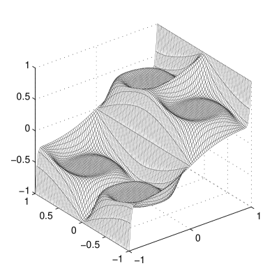
  (a) A $3D$ plot of the function $y_{1}+\chi_{1}(y_{1},y_{2})$.

  

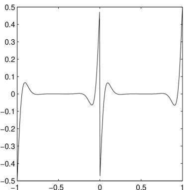
  (b) The cross-section of the plot of the function $y_{1}+\chi_{1}(y_{1},y_{2})-\tfrac{1}{2}\operatorname{sign}y_{1}$ at $y_{1}=1/2$.

  Figure 3: Two plots indicating that $\chi_{1}+y_{1}-\frac{1}{2}\operatorname{sign}(y_{1})$ is small in cell interiors.

With this explanation, we proceed to estimate each function individually, starting with $\eta$. Since $\nabla\cdot v=0$, Lemma 2.7 guarantees

$$\lVert\eta\rVert_{L^{\infty}}\leqslant c\lVert\nabla\chi_{1}\rVert_{L^{2}}.$$

We remark that while Lemma 2.7 is stated for homogeneous Dirichlet boundary conditions, the proof in [bblBerestyckiKiselevNovikovRyzhik] goes through verbatim for periodic boundary conditions, provided, of course, we assume our solution is mean-zero. This justifies the application of Lemma 2.7 in this context.

Since we know from [bblFannjiangPapanicolaou] that $\lVert\nabla\chi_{1}\rVert_{L^{2}}=O(A^{1/4})$, we immediately obtain

$$\lVert\eta\rVert_{L^{\infty}}\leqslant cA^{1/4}.$$ (4.14)

Our bound for $\psi_{1}$ is similar in flavor. Let $\xi_{i}=\chi_{i}+y_{i}-\frac{1}{2}\operatorname{sign}(y_{i})$. Then for any $p\geqslant 1$, we know from [bblFannjiangPapanicolaou] (see also [bblNovikovPapanicolaouRyzhik]*Theorem 1.2) that

$$\lVert\xi_{i}\rVert_{L^{p}}\leqslant cA^{-\frac{1}{2p}}.$$

Since $-A\langle v_{i}\chi_{i}\rangle=O(\sqrt{A})$, from Lemma 2.7 we have

$$\lVert\psi_{1}\rVert_{L^{\infty}}\leqslant cA\left(\lVert\xi_{i}\rVert_{L^{p}}+\sum_{i=1}^{2}\left\lvert\left\langle v_{i}\chi_{i}\right\rangle\right\rvert\right)\leqslant cA^{1-\frac{1}{2p}}$$ (4.15)

for any $p>1$.

Finally for $\psi_{2}$, our aim is to absorb the right hand side into the drift. For $i=1,2$, Let $f_{i}=f_{i,A}$ be defined by

$$f_{i}(y)=\frac{y_{i}^{2}-\lvert y_{i}\rvert}{2}\qquad\text{if }\frac{1}{\sqrt{A}}\leqslant\lvert y_{i}\rvert\leqslant 1-\frac{1}{\sqrt{A}},$$

and extended to be a $C^{1}$, periodic function on $\mathbb{R}^{2}$ in the natural way. Set $\theta=\psi_{2}+\sum_{i=1}^{2}(f_{i}-\langle f_{i}\rangle)$, then $\theta$ is a periodic, mean-zero solution to

$$-\Delta_{y}\theta+Av\cdot\nabla_{y}\theta=\sum_{i=1}^{2}\left(Av_{i}g_{i}-\Delta_{y}f_{i}\right).$$

where

$$g_{i}(y)=\partial_{y_{i}}f_{i}-y_{i}+\frac{1}{2}\operatorname{sign}(y_{i})$$

Since for any $p\geqslant 1$, we can explicitly compute

$$\lVert g_{i}\rVert_{L^{p}}\leqslant cA^{-\frac{1}{2p}}\quad\text{and}\quad\lVert\Delta_{y}f_{i}\rVert_{L^{p}}\leqslant cA^{\frac{1}{2}-\frac{1}{2p}},$$

by Lemma 2.7 we obtain

$$\lVert\psi_{2}\rVert_{L^{\infty}}\leqslant 1+\lVert\theta\rVert_{L^{\infty}}\leqslant cA^{1-\frac{1}{2p}}$$ (4.16)

for any $p>1$.

Thus combining (4.14), (4.15) and (4.16), we see $\lVert\tau_{12}\rVert_{L^{\infty}}\leqslant cA^{1-1/(2p)}$. Thus using (1.14) and choosing $p=\frac{8-2\alpha}{8-3\alpha}$ when $0<\alpha<8/3$, and $p=\infty$ for $\alpha\geqslant 8/3$, we see

$$\frac{\lVert\tau_{12}\rVert_{L^{\infty}}}{L^{2}}\leqslant cL^{-\frac{\alpha}{4}}$$

proving (4.12). This completes the proof. ∎

Exit time from a square.

Theorem 1.4 follows immediately from Proposition 1.4.

• The proof of Theorem 1.4 is now trivial. We simply inscribe a disk $\underline{D}=\{|x|\leqslant L/2\}$ into the square $D=[-L/2,L/2]^{2}$, and circumscribe a bigger disk $\overline{D}=\{\lvert x\rvert\leqslant L/\sqrt{2}\}$ around $D$. The corresponding exit times satisfy the inequality

  $$\underline{\tau}(x)\leqslant\tau(x)\leqslant\overline{\tau}(x),\quad\text{for all $x\in\underline{D}$.}$$

  Using the bounds obtained from Proposition 1.5 applied to $\underline{D}$ and $\overline{D}$, the inequality (1.20) follows. ∎

5 The eigenvalue in the homogenization regime

5.1 The lower bound

The lower bound for the eigenvalue stated in Theorem 1.2 follows, quickly from the upper bound on the expected exit time.

• We claim that in general, we have the principal eigenvalue and expected exit time satisfy

  $$\lambda\geqslant\frac{1}{\|\tau\|_{L^{\infty}}}.$$ (5.1)

  To see this, pick any $\varepsilon>0$, and suppose for contradiction that $\lambda<1/\lVert\tau+\varepsilon\rVert_{L^{\infty}}$. Then,

  $$-\Delta(\tau+\varepsilon)+Av\cdot\nabla(\tau+\varepsilon)=1\geqslant\frac{1}{\|\tau+\varepsilon\|_{L^{\infty}}}\left(\tau+\varepsilon\right).$$

  Also

  $$-\Delta\varphi+Av\cdot\nabla\varphi=\lambda\varphi\leqslant\frac{1}{\lVert\tau+\varepsilon\rVert_{L^{\infty}}}\varphi.$$

  Rescaling $\varphi$ if necessary to ensure $\lVert\varphi\rVert_{L^{\infty}}\leqslant\varepsilon$, we see have $\varphi\leqslant\tau+\varepsilon$ in $D$. Thus Perron’s method implies the existence of a function $\phi$ such that c?s - Δϕ+ A v ⋅∇ϕ= 1∥τ+ ε∥L∞ ϕ& in $D$,
  ϕ= 0 on $\partial D$,
  φ⩽ϕ⩽τ in $D$ This immediately implies $1/\lVert\tau+\varepsilon\rVert_{L^{\infty}}$ equals the principal eigenvalue $\lambda$, which contradicts our assumption. Thus, for any $\varepsilon>0$, we must have $\lambda\geqslant 1/\lVert\tau+\varepsilon\rVert_{L^{\infty}}$. Sending $\varepsilon\to 0$, we obtain (5.1). Applying Theorem 1.4 concludes the proof. ∎

5.2 The upper bound

In this section we prove the upper bound in Theorem 1.2. We will do this by using a multi-scale expansion of a sub-solution. As we have seen in the preceding sections, our multi-scale expansions are all forced to use a quadratic ‘slow’ profile, in order to avoid extra terms in the expansion. This makes the construction of the sub-solution slightly more difficult. As customary with homogenization problems, we rescale the problem so that the cell size goes to $0$, and the domain is fixed.

Lemma 5.1.

Let $h>0$, and $\psi$ be the solution of

$$\left\{\begin{aligned} -\Delta\psi+ALv(Lx)\cdot\nabla\psi&=\chi_{B_{1-h}}&&\text{in }B_{1}\\ \psi&=0&&\text{on }\partial B_{1},\\ \end{aligned}\right.$$ (5.2)

where $B_{r}=\{|x|\leqslant r\}$, and $\chi_{S}$ is the characteristic function of the set $S$. Assume that $A$ and $L$ vary such that (1.14) holds. Then there exists $h>0$, and $c=c(h)>0$ such that

$$\psi(x)\geqslant\frac{c}{\sqrt{A}}\quad\text{for all }x\in B_{1-h}.$$ (5.3)

provided $A$ and $L$ are sufficiently large.

Lemma 5.1 immediately implies the desired upper bound. We present this argument below before delving into the technicalities of Lemma 5.1.

• Let $\varphi_{1}$, $\mu_{1}$ be the principal eigenfunction and the principal eigenvalue respectively for the rescaled problem

  $$\left\{\begin{aligned} -\Delta\varphi_{1}+ALv(Lx)\cdot\nabla\varphi_{1}&=\mu_{1}\varphi_{1}&&\text{in }B_{1}\\ \varphi_{1}&=0&&\text{on }\partial B_{1},\\ \varphi_{1}&>0&&\text{in }B_{1}.\end{aligned}\right.$$ (5.4)

  Assume, for contradiction, $\mu_{1}>\frac{\sqrt{A}}{c}$, where $c$ is the constant in Lemma 5.1, then

  $$-\Delta\varphi_{1}+ALv(Lx)\cdot\nabla\varphi_{1}=\mu_{1}\varphi_{1}\geqslant\frac{\sqrt{A}}{c}\varphi_{1}.$$

  Also, if $\psi$ is the function from Lemma 5.1, then by the maximum principle, $\psi>0$ in $B_{1-h}$. Hence,

  $$-\Delta\psi+ALv(Lx)\cdot\nabla\psi=\chi_{B_{1-h}}\leqslant\frac{\sqrt{A}}{c}\psi.$$

  By the Hopf lemma, we know $\frac{\partial\varphi_{1}}{\partial n}<0$ on $\partial B_{1}$, and so $\varphi_{1}$ can be rescaled to ensure $\varphi_{1}\geqslant\psi$. Perron’s method now implies that there exists a function $\phi$ that satisfies

  $$\left\{\begin{aligned} -\Delta\phi+ALv(Lx)\cdot\nabla\phi&=\frac{\sqrt{A}}{c}\phi&&\text{in }B_{1}\\ \phi&=0&&\text{on }\partial B_{1},\\ \phi&>0&&\text{in }B_{1},\end{aligned}\right.$$ (5.5)

  and, in addition, $\psi(x)\leqslant\phi(x)\leqslant\varphi_{1}(x)$. Therefore, $\mu_{1}=\sqrt{A}/c$ is the principal eigenvalue, which contradicts our assumption $\mu_{1}>\sqrt{A}/c$. Hence $\mu_{1}\leqslant\sqrt{A}/c$.

  Now rescaling back so the cell size is $1$, let $\lambda^{\prime}$ and $\phi^{\prime}$ be the principal eigenvalue and principal eigenfunction respectively of the problem (1.11) on the ball of radius $L/2$. Since $\lambda^{\prime}=4\mu_{1}/L^{2}$, we have $\lambda^{\prime}\leqslant 4\sqrt{A}/(cL^{2})$. Finally, let $D$ be the square with side length $L$, and $\lambda$, $\varphi$ are the principal eigenvalue and eigenfunction respectively of the problem (1.11) on $D$. Then, since $B_{L/2}\subset D$, the principal eigenvalues must satisfy $\lambda\leqslant\lambda^{\prime}$, from which the theorem follows. ∎

It remains to prove Lemma 5.1.

• Let $\theta=\tau_{1}-\psi$, where $\tau_{1}$ is the solution of (4.1), the expected exit time problem from the unit disk. Now rescaling (1.21) to the ball of radius $1$, (or directly using (4.11), which was what lead to (1.21)), we obtain

  $$\left\lvert\tau_{1}(x)-\frac{1}{2\operatorname{tr}(\bar{\sigma}(A))}\left(1-\lvert x\rvert^{2}\right)\right\rvert\leqslant\frac{c_{3}L^{-\alpha/4}}{\sqrt{A}}$$ (5.6)

  provided $A$ and $L$ are large enough and satisfy (1.14). Here $c_{3}>0$ is a fixed constant independent of $A$ and $L$. Thus, (5.3) will follow if we show that

  $$\lVert\theta\rVert_{L^{\infty}(B_{1-h})}\leqslant(1-\varepsilon^{\prime})\inf_{x\in B_{1-h}}\tau_{1}(x)$$ (5.7)

  for some small $\varepsilon^{\prime}>0$. Observe that (5.6) implies that the right hand side of (5.7) is $O(h/\sqrt{A})$. Therefore, to establish (5.7), it suffices to show that there exists constants $h_{0}>0$ and $c>0$ such that for all $h\leqslant h_{0}$, there exists $A_{0}=A_{0}(h)$ and $L_{0}=L_{0}(h)$ such that

  $$\lVert\theta\rVert_{L^{\infty}(B_{1-h})}\leqslant\frac{c}{\sqrt{A}}h^{3/2},$$ (5.8)

  provided $A\geqslant A_{0}$, $L\geqslant L_{0}$ and (1.14) holds. Above any power of $h$ strictly larger than $1$ will do; our construction below obtains $h^{3/2}$, however, in reality one would expect the power to be $h^{2}$.

  We will obtain (5.8) by considering a Poisson problem on the annulus

  $$\mathcal{A}_{1-2h,1}=\{1-2h\leqslant|x|\leqslant 1\}.$$

  If we impose a large enough constant boundary condition on the inner boundary, the (inward) normal derivative will be negative on $\partial B_{1-2h}$. Now, if we extend this function inward by a constant, we will have a super-solution giving the desired estimate for $\theta(x)$. We first state a lemma guaranteeing the sign of the normal derivative of an appropriate Poisson problem.

  Lemma 5.2.

  There exists $h_{0}$ and $c_{2}>0$, such that for all $h<h_{0}$, there exists $A_{0}$, $L_{0}>0$ such that the solution $\theta_{1}$ of the PDE

  $$\left\{\begin{aligned} -\Delta\theta_{1}+ALv(Lx)\cdot\nabla\theta_{1}&=\chi_{\mathcal{A}_{1,1-h}}&&\text{in }\mathcal{A}_{1-2h,1}\\ \theta_{1}&=0&&\text{on }\partial B_{1},\\ \theta_{1}&=\frac{c_{2}}{\sqrt{A}}h^{3/2}&&\text{on }\partial B_{1-2h},\\ \end{aligned}\right.$$ (5.9)

  satisfies

  $$\frac{\partial\theta_{1}}{\partial r}\leqslant 0\quad\text{on }\partial B_{1-2h},$$

  provided $L\geqslant L_{0}$, $A\geqslant A_{0}$ and (1.14) holds. Here $\frac{\partial}{\partial r}$ denotes the derivative with respect to the radial direction. Moreover, the function $\theta_{1}$ attains its maximum on $|x|=1-2h$, and $\theta_{1}(x)\leqslant{c_{2}}h^{3/2}/{\sqrt{A}}$ for all $x\in\mathcal{A}_{1-2h,1}$.

Now, postponing the proof of Lemma 5.2, we prove (5.8). Choose $h$ small, and $A,L$ large, as guaranteed by Lemma 5.2, and define $\bar{\theta}$ by

$$\bar{\theta}(x)=\begin{dcases}\theta_{1}(x)&\text{when }\lvert x\rvert\geqslant 1-2h\\ \frac{c_{2}}{\sqrt{A}}h^{3/2}&\text{when }\lvert x\rvert<1-2h.\end{dcases}$$

where $\theta_{1}$ and $c_{2}$ are as in Lemma 5.2. Then $\bar{\theta}\in C(B_{1})\cap C^{2}(B_{1-2h}\cup\mathcal{A}_{1-2h,1})$, and

$$\left(-\Delta+ALv(Lx)\cdot\nabla\right)\bar{\theta}(x)=\begin{dcases}1&\text{when }\lvert x\rvert\geqslant 1-h\\ 0&\text{when }\lvert x\rvert<1-h\;\&\;\lvert x\rvert\neq 1-2h\end{dcases}$$

Further, when $\lvert x\rvert=1-2h$,

$$\frac{\partial\bar{\theta}}{\partial r^{-}}=0\quad\text{and}\quad\frac{\partial\bar{\theta}}{\partial r^{+}}\leqslant 0$$

where the second inequality follows from Lemma 5.2. Thus $\bar{\theta}$ is a viscosity super solution to the PDE

$$\left\{\begin{aligned} -\Delta\theta+ALv(Lx)\cdot\nabla\theta&=\chi_{\mathcal{A}_{1,1-h}}&&\text{in }B_{1}\\ \theta&=0&&\text{on }\partial B_{1}.\end{aligned}\right.$$

By the comparison principle, we must have $\bar{\theta}\geqslant\theta$, which immediately proves (5.8). From this (5.7) follows, and using (5.6) we obtain (5.2), concluding the proof. ∎

It remains to prove Lemma 5.2. Roughly speaking, if we choose the constant $c_{2}$ sufficiently large, the function $\theta_{1}$ is nearly harmonic. The inhomogeneity of the boundary conditions dominates the right side of the equation. A “nearly harmonic” function should attain its maximum on the boundary, implying the conclusion of Lemma 5.2.

The reason we believe the constant $c_{2}h^{3/2}/\sqrt{A}$ is large enough, is because the homogenized exit time from the annulus is quadratic in the width of the annulus. Unfortunately, the slow profile is not quadratic in Cartesian coordinates, and so the best we can do is obtain upper and lower bounds, which need not be sharp. We begin by showing that the expected exit time from an annulus of width $h$ grows like $h^{3/2}$. While we certainly don’t expect the exponent $3/2$ to be sharp, any exponent strictly larger than $1$ will suffice for our needs.

Lemma 5.3.

Let $\mathcal{A}_{1-h,1}$ be the annulus $\mathcal{A}_{1-h,1}\stackrel{{\scriptstyle\text{def}}}{{=}}B_{1}\setminus B_{1-h}$, and $\tau_{\text{ann}}$ be the solution of the Poisson problem

$$\left\{\begin{aligned} -\Delta\tau_{\text{ann}}+ALv(Lx)\cdot\nabla\tau_{\text{ann}}&=1&&\text{in }\mathcal{A}_{1-h,1}\\ \tau_{\text{ann}}&=0&&\text{on }\partial\mathcal{A}_{1-h,1}\end{aligned}\right.$$ (5.10)

Suppose $L$ and $A$ vary so that (1.14) holds. Then there exists constants $h_{0}>0$ and $c>0$ such that for all $h<h_{0}$, there exists $A_{0}=A_{0}(h)$ and $L_{0}=L_{0}(h)$ such that

$$\lVert\tau_{\text{ann}}\rVert_{L^{\infty}(\mathcal{A}_{1-h,1})}\leqslant\frac{c_{1}}{\sqrt{A}}h^{3/2}$$

provided $L\geqslant L_{0}$, $A\geqslant A_{0}$ and (1.14) holds.

• The main idea behind the proof is that as $A,L\to\infty$, we know that $\tau_{1}$ tends to an explicit (homogenized) parabolic profile and is constant on $\partial B_{1-h}$. Now if we subtract off a harmonic function with these boundary values, then we should get a super solution for $\tau_{\text{ann}}$. Finally, we will show that a harmonic function with constant boundary values grows linearly near $\partial B_{1}$, at the same rate as $\tau_{1}$. Thus the above super solution will give an upper bound for $\tau_{\text{ann}}$ which is super-linear in the annulus width.

  We proceed to carry out the details. Let $\eta^{\prime}$ be the solution of

  $$\left\{\begin{aligned} -\Delta\eta^{\prime}+ALv(Lx)\cdot\nabla\eta^{\prime}&=0&&\text{in }\mathcal{A}_{1-h,1}\\ \eta^{\prime}&=0&&\text{on }\partial B_{1}\\ \eta^{\prime}&=\frac{2h-h^{2}}{2\operatorname{tr}(\bar{\sigma}(A))}&&\text{on }\partial B_{1-h},\end{aligned}\right.$$ (5.11)

  and define

  $$\bar{\tau}_{\text{ann}}=\tau_{1}-\eta^{\prime}+\frac{c_{3}L^{-\alpha/4}}{\sqrt{A}},$$

  where $c_{3}$ is as in (5.6). Then $\bar{\tau}_{\text{ann}}$ satisfies

  $$\left\{\begin{aligned} -\Delta\bar{\tau}_{\text{ann}}+ALv(Lx)\cdot\nabla\bar{\tau}_{\text{ann}}&=1&&\text{in }\mathcal{A}_{1-h,1}\\ \bar{\tau}_{\text{ann}}&\geqslant 0&&\text{on }\partial B_{1}\\ \bar{\tau}_{\text{ann}}&\geqslant 0&&\text{on }\partial B_{1-h}.\end{aligned}\right.$$

  The first boundary condition follows because both $\eta^{\prime}$ and $\tau_{1}$ are $0$ on $\partial B_{1}$. The second follows from (5.6) and the boundary condition for $\eta^{\prime}$. Thus, the maximum principle immediately implies that $\bar{\tau}_{\text{ann}}\geqslant\tau_{\text{ann}}$.

  Since (5.6) gives the asymptotics for $\tau_{1}$, to conclude the proof we need a lower bound on $\eta^{\prime}$ that is ‘linear’ in the radial direction near $\partial B_{1}$. We separate this estimate as a lemma.

  Lemma 5.4.

  Let $\eta$ be the solution of

  $$\left\{\begin{aligned} -\Delta\eta+ALv(Lx)\cdot\nabla\eta&=0&&\text{in }\mathcal{A}_{1-h,1}\\ \eta&=0&&\text{on }\partial B_{1}\\ \eta&=h&&\text{on }\partial B_{1-h},\end{aligned}\right.$$ (5.12)

  Then there exists a constant $c$, independent of $h$, $A$ and $L$, such that

  $$\eta(x)\geqslant 1-\lvert x\rvert-c\left(h^{3/2}+\frac{L^{-\alpha/4}}{\sqrt{h}}\right)$$ (5.13)

  when $L$ and $A$ are sufficiently large.

  Returning to the proof of Lemma 5.3, we see that Lemma 5.4 gives

  $$\eta^{\prime}(x)\geqslant\frac{2-h}{2\operatorname{tr}(\bar{\sigma}(A))}\left[1-\lvert x\rvert-c\left(h^{3/2}+\frac{L^{-\alpha/4}}{\sqrt{h}}\right)\right].$$

  Now using the above and (1.8), it follows that

  $$\tau_{\text{ann}}(x) \leqslant\bar{\tau}_{\text{ann}}(x)=\tau_{1}(x)-\eta^{\prime}(x)+\frac{cL^{-\alpha/4}}{\sqrt{A}}$$

  $$\leqslant\frac{1}{2\operatorname{tr}(\bar{\sigma}(A))}\left(1-\lvert x\rvert^{2}-(2-h)(1-\lvert x\rvert)+ch^{3/2}\right)+\frac{1}{\sqrt{A}}\left(cL^{-\alpha/4}+\frac{cL^{-\alpha/4}}{\sqrt{h}}\right)$$

  $$=\frac{1}{2\operatorname{tr}(\bar{\sigma}(A))}\left(\left(1-\lvert x\rvert\right)\left(h-(1-\lvert x\rvert)\right)+ch^{3/2}\right)+\frac{1}{\sqrt{A}}\left(\frac{cL^{-\alpha/4}}{\sqrt{h}}\right)$$

  $$\leqslant\frac{1}{2\operatorname{tr}(\bar{\sigma}(A))}\left(h^{2}+ch^{3/2}\right)+\frac{1}{\sqrt{A}}\left(\frac{cL^{-\alpha/4}}{\sqrt{h}}\right)$$

  obtaining Lemma 5.3 as desired. ∎

To complete the proof of Lemma 5.3, we need to prove Lemma 5.4. We do this next.

• We will construct a sub-solution of equation (5.12) in small rectangles overlapping $\mathcal{A}_{1-h,1}$. For convenience, we now shift the origin to $(-1,0)$, and consider new coordinates $(x_{1}^{\prime},x_{2}^{\prime})\stackrel{{\scriptstyle\text{def}}}{{=}}(x_{1}+1,x_{2})$. In these coordinates, let $R$ be the rectangle of height $2h^{3/4}$, width $h$ and top left corner $(\rho_{0},h^{3/4})$, where $\rho_{0}=1-(1-h^{3/2})^{1/2}$ (see Figure 4).

  

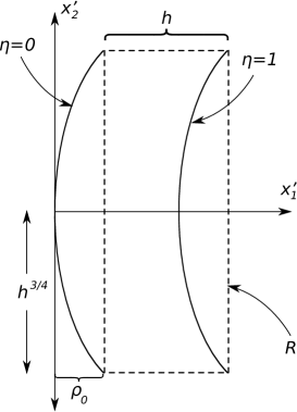
  Figure 4: Domain for $\eta_{\text{sub}}$.

We will construct a function $\eta_{\text{sub}}$ such that

$$\left\{\begin{aligned} -\Delta\eta_{\text{sub}}+ALv(Lx)\cdot\nabla\eta_{\text{sub}}&=0&&\text{in }\mathcal{A}_{1-h,1},\\ \eta_{\text{sub}}&\leqslant h&&\text{on the right boundary of }R,\\ \eta_{\text{sub}}&\leqslant 0&&\text{on the other three boundaries of }R,\end{aligned}\right.$$ (5.14)

and $\eta_{\text{sub}}$ satisfies the linear growth condition

$$\eta_{\text{sub}}(x_{1}^{\prime},0)\geqslant x_{1}^{\prime}-c\left(h^{3/2}+\frac{L^{-\alpha/4}}{\sqrt{h}}\right)\quad\text{when }x_{1}^{\prime}\in[\rho_{0},\rho_{0}+h],$$ (5.15)

for some constant $c$ independent of $L$, $A$ and $h$.

Before proving that the function $\eta_{\text{sub}}$ exists, we remark that by the maximum principle, we $\eta_{\text{sub}}\leqslant\eta$ on $R\cap\mathcal{A}_{1-h,h}$. Moreover, as $\rho_{0}=O(h^{3/2})$, the estimate (5.13) can be extended to $x_{1}^{\prime}\in[0,\rho_{0}]$ as well, possibly by increasing the constant $c$. This proves Lemma 5.4 when $x$ is on the negative $x_{1}$-axis. Now, if (5.15) is still valid when the coordinate frame is rotated, our proof of Lemma 5.4 will be complete!

We will first prove that a function $\eta_{\text{sub}}$ satisfying (5.14) and (5.15) exists. We will do this by a multi-scale expansion. Let

$$\eta_{\text{sub}}(x^{\prime})=\eta_{0}(x^{\prime})+\frac{1}{L}\eta_{1}(x^{\prime},y)+\frac{1}{L^{2}}\eta_{2}(y)-\frac{c_{0}L^{-\alpha/4}}{\sqrt{h}},$$

where $y=Lx^{\prime}$ is the fast variable, $\eta_{0}$ is given by

$$\eta_{0}(x_{1}^{\prime},x_{2}^{\prime})=x_{1}^{\prime}-c_{1}\rho_{0}+\frac{((x_{1}^{\prime})^{2}-(x_{2}^{\prime})^{2})}{\sqrt{h}},$$

and $c_{0}$, and $c_{1}$ are constants, each independent of $L$, $A$ and $h$, to be chosen later. As before, $\eta_{1}$ is

$$\eta_{1}(x^{\prime},y)=\sum_{i=1}^{2}\chi_{i}(y)\partial_{x_{i}^{\prime}}\eta_{0}(x^{\prime}),$$

and $\eta_{2}$ is the mean $0$, periodic solution to

$$-\Delta_{y}\eta_{2}+Av(y)\cdot\nabla_{y}\eta_{2}=\sum_{i=1}^{2}\left[2\partial_{y_{i}}\chi_{j}-A\left(v_{i}\chi_{j}-\langle v_{i}\chi_{j}\rangle\right)\right]\partial_{x_{i}^{\prime}}\partial_{x_{j}^{\prime}}\eta_{0},$$ (5.16)

where $\chi_{i}$ are the solutions to (4.7).

Again, the crucial fact here is that since $\eta_{0}$ is quadratic, the second derivatives are constant and $\eta_{2}$ becomes independent of the slow variable $x^{\prime}$. Using this, a direct computation shows that

$$-\Delta\eta_{\text{sub}}+ALv\cdot\nabla\eta_{\text{sub}}=-\Delta\eta_{0}+A\sum_{i,j}\langle v_{i}\chi_{j}\rangle\partial_{x_{i}^{\prime}}\partial_{x_{j}^{\prime}}\eta_{0}.$$ (5.17)

Note that by symmetry, $\langle v_{1}\chi_{1}\rangle=\langle v_{2}\chi_{2}\rangle$, and $\langle v_{1}\chi_{2}\rangle=\langle v_{2}\chi_{1}\rangle=0$. Further, by our choice of $\eta_{0}$, we have $\Delta\eta_{0}=0$. Hence, the previous equation reduces to

$$-\Delta\eta_{\text{sub}}+ALv\cdot\nabla\eta_{\text{sub}}=0,$$

as required by the first equation in (5.14).

Next, we show that if $c_{1}$ is appropriately chosen, we can arrange the boundary conditions claimed in (5.14) for $\eta_{0}$. Notice that $\rho_{0}=O(h^{3/2})$, and on the top and bottom boundary we have $x_{2}^{\prime}=\pm h^{3/4}$ and $x_{1}^{\prime}\in(\rho_{0},\rho_{0}+h)$. Thus

$$x_{1}^{\prime}-\frac{(x_{2}^{\prime})^{2}}{\sqrt{h}}\leqslant\rho_{0}\quad\text{and}\quad\frac{(x_{1}^{\prime})^{2}}{\sqrt{h}}\leqslant O(h^{3/2}).$$

So choosing $c_{1}$ large enough, we can ensure $\eta_{0}\leqslant 0$ on the top and bottom of $R$.

On the left of $R$, we have $x_{1}^{\prime}=\rho_{0}$ and $\lvert x_{2}\rvert\leqslant h^{3/4}$. So $(x_{1}^{\prime})^{2}/\sqrt{h}\leqslant O(h^{5/2})=o(\rho_{0})$, and choosing $c_{1}$ large we can again ensure $\eta_{0}\leqslant 0$ on the left of $R$. Finally, on the right of $R$, we have $x_{1}^{\prime}=\rho_{0}+h$ and $\lvert x_{2}^{\prime}\rvert\leqslant h^{3/4}$, and we immediately see that for $c_{1}$ large enough, we have $\eta_{0}\leqslant h$ on the right of $R$. Thus $\eta_{0}$ satisfies the boundary conditions in (5.14).

To see that $\eta_{\text{sub}}$ also satisfies the boundary conditions in (5.14), we need to bound the correctors appropriately. Exactly as in the proof of Lemma 4.1, we obtain

$$\left\lVert\frac{1}{L}\eta_{1}+\frac{1}{L^{2}}\eta_{2}\right\rVert_{L^{\infty}}\leqslant\frac{cL^{-\alpha/4}}{\sqrt{h}},$$ (5.18)

where $c>0$ is independent of $L$, $A$ and $h$. We remark that the extra ${1}/{\sqrt{h}}$ factor arises because derivatives of $\eta_{0}$ are of the order ${1}/{\sqrt{h}}$ and they appear as multiplicative factors in the expressions for $\eta_{1}$ and $\eta_{2}$.

Consequently, if $c_{0}$ is chosen to be larger than $c$, we have

$$\frac{1}{L}\eta_{1}+\frac{1}{L^{2}}\eta_{2}-\frac{c_{0}L^{-\alpha/4}}{\sqrt{h}}\leqslant 0.$$ (5.19)

Since $\eta_{0}$ already satisfies the boundary conditions in (5.14), this immediately implies that $\eta_{\text{sub}}$ must also satisfy these boundary conditions. Finally, since $\eta_{0}$ certainly satisfies (5.15), it follows from (5.19) that $\eta_{\text{sub}}$ also satisfies (5.15). This proves the existence of $\eta_{\text{sub}}$.

Now, as remarked earlier, the only thing remaining to complete the proof of the Lemma is to verify that if the rectangle $R$, and the coordinate frame are both rotated arbitrarily about the center of the annulus, then there still exists a function $\eta_{\text{sub}}$ satisfying (5.14) and (5.15) in new coordinates. This, however, is immediate. The new coordinates can be expressed in terms of the old coordinates as a linear function. Consequently, our initial profile for $\eta_{0}$ will still be a quadratic function of the new coordinates. Of course, by the rotational invariance of the Laplacian, it will also be harmonic, and the remainder of the proof goes through nearly verbatim. The only modification is that after the rotation the mixed derivative $\partial_{x_{1}^{\prime}}\partial_{x_{2}^{\prime}}\eta_{0}$ no longer vanishes, and the terms involving $v_{1}\chi_{2}$ and $v_{2}\chi_{1}$ do appear in (5.16) and (5.17). However, they can be treated in an identical fashion, as in the proof of Lemma  4.1 using the precise asymptotics for $\chi_{1}$ and $\chi_{2}$ from [bblNovikovPapanicolaouRyzhik]. This concludes the proof. ∎

Finally, we are ready for the proof of Lemma 5.2.

• For a given $c_{2}$, let $\eta^{\prime}$ be the solution of

  $$\left\{\begin{aligned} -\Delta\eta^{\prime}+ALv(Lx)\cdot\nabla\eta^{\prime}&=0&&\text{in }\mathcal{A}_{1-2h,1}\\ \eta^{\prime}&=0&&\text{on }\partial B_{1}\\ \eta^{\prime}&=\frac{c_{2}}{\sqrt{A}}h^{3/2}&&\text{on }\partial B_{1-2h},\end{aligned}\right.$$

  Then, we have

  $$\theta_{1}-\eta^{\prime}=0\hbox{ on $\partial\mathcal{A}_{1-2h,1}$},$$

  and

  $$-\Delta\theta_{1}+ALv(Lx)\cdot\nabla\theta_{1}\leqslant 1\hbox{ in $\mathcal{A}_{1-2h,1}$.}$$

  Consequently $\theta_{1}-\eta^{\prime}\leqslant\tau_{\text{ann}}$, where $\tau_{\text{ann}}$ is the solution of (5.10) on the annulus $\mathcal{A}_{1-2h,1}$. Thus applying Lemma 5.3, we see

  $$\theta_{1}(x)\leqslant\frac{c_{1}}{\sqrt{A}}(2h)^{3/2}+\eta^{\prime}(x)$$ (5.20)

  The function $\eta^{\prime}$ decreases at most linearly with $\lvert x\rvert$. This can be seen immediately from an asymptotic expansion for a super solution. Indeed, starting with

  $$\eta_{0}(x)=\frac{c_{2}\sqrt{h}}{2\sqrt{A}}(1-x_{1})$$

  and choosing $\eta_{1}$ and $\eta_{2}$ as in the proof of Lemma 5.4, we immediately see that

  $$\eta^{\prime}(x_{1},0)\leqslant\frac{c_{2}\sqrt{h}}{2\sqrt{A}}(1-x_{1})+c\sqrt{h}A^{-1/2}L^{-\alpha/4}.$$

  We remark again that the extra $\sqrt{h}A^{-1/2}$ factor arises from the gradient of $\eta_{0}$. Now by rotating the initial profile $\eta_{0}$ appropriately, we obtain the linear decrease

  $$\eta^{\prime}(x)\leqslant\frac{c_{2}\sqrt{h}}{2\sqrt{A}}(1-\lvert x\rvert)+c\sqrt{h}A^{-1/2}L^{-\alpha/4}.$$ (5.21)

  as claimed.

  We claim that (5.20) and (5.21) quickly conclude the proof. To see this, note first that equation (5.20) and (5.21) immediately give

  $$\theta_{1}(x)\leqslant\frac{c_{1}}{\sqrt{A}}(2h)^{3/2}+\frac{c_{2}}{2\sqrt{A}}h^{3/2}+c\sqrt{h}A^{-1/2}L^{-\alpha/4}\quad\text{whenever }x\in\mathcal{A}_{1-h,1}.$$ (5.22)

  However, since

  $$-\Delta\theta_{1}+ALv(Lx)\cdot\nabla\theta_{1}=0$$

  on $\mathcal{A}_{1-2h,1-h}$, the maximum principle implies that $\theta_{1}$ can not attain it’s maximum in the interior of the annulus $\mathcal{A}_{1-2h,1-h}$. Consequently (5.22) must hold on the interior of the entire annulus $\mathcal{A}_{1-2h,1}$.

  Now if we choose $c_{2}$ large enough so that $2^{3/2}c_{1}<\frac{c_{2}}{4}$, and then choose $L,A$ large enough so that $cA^{-1/2}L^{-\alpha/4}<\frac{c_{2}}{4}$, we see that $\theta_{1}$ is forced to attain it’s maximum on the inner boundary $\partial B_{1-2h}$, and the Lemma follows immediately. ∎