The Morris-Lecar neuron model embeds a leaky integrate-and-fire model

Abstract

We show that the stochastic Morris-Lecar neuron, in a neighborhood of its stable point, can be approximated by a two-dimensional Ornstein-Uhlenbeck (OU) modulation of a constant circular motion. The associated radial OU process is an example of a leaky integrate-and-fire (LIF) model prior to firing. A new model constructed from a radial OU process together with a simple firing mechanism based on detailed Morris-Lecar firing statistics reproduces the Morris-Lecar Interspike Interval (ISI) distribution, and has the computational advantages of a LIF. The result justifies the large amount of attention paid to the LIF models.

Ditlevsen and Greenwood

[University of Copenhagen]Susanne Ditlevsen [University of British Columbia and University of Copenhagen]Priscilla Greenwood

Department of Mathematical Sciences, Universitetsparken 5, DK-2100 Copenhagen Ø, email: susanne@math.ku.dk

Mathematics Annex 1208 2329W East Mall, Vancouver, BC V6T 1Z4, Canada, email: pgreenw@math.la.asu.edu

60G9937N25

1 Introduction

Much effort has been made to create a realistic but still easily computed stochastic neuron model, primarily by combining subthreshold dynamics with firing rules. The result has been a variety of, usually one dimensional, leaky integrate-and-fire (LIF) descriptions with a fixed membrane potential firing threshold [4, 11, 18, 19], or with a rate of firing depending more sensitively on membrane potential [15, 21]. These models are useful both for obtaining analytical results and for ease of simulation.

By contrast, the two-dimensional stochastic Morris-Lecar (ML) neuron model, a simple cousin to the more detailed Hodgkin-Huxley (HH) model, describes the dynamics of firing in a way more closely motivated by the biology. It has been better respected by biologists than the LIF class of models, but has received little attention owing to the difficulty of mathematical analysis of this rather complicated stochastic dynamical system.

In Section 4 of this paper we show that in fact a LIF model is embedded in the ML model as an integral part of it, closely approximating the subthreshold fluctuations of the ML dynamics. This result suggests that perhaps the firing pattern of a stochastic ML can be recreated using the embedded LIF together with a ML stochastic firing mechanism. We construct such a model in Section 5 and 6, and show in Section 7 that its Interspike Interval (ISI) distribution is similar to that of the ML. Our model, while of the type described in our first paragraph, combines the realism of the ML with the ease of analysis and computation of a one dimensional LIF-type model. The work invested in LIF models is further justified by this new model.

Before we set up our stochastic ML model and write analytical details, let us have an informal look at how it works. The principal dynamics of the ML, in the central range of the input current, consist of a stable limit cycle (Fig. 1A) corresponding to firing, which encloses a stable fixed point. In between there loops an unstable limit cycle. The path of the stochastic model has two quasi-stable patterns (Fig. 1B). One is succesive firings, where the dynamics makes “large” noisy circuits around the stable limit cycle, the other is membrane fluctuations between spikes, where the dynamics makes “small” noisy circuits around the fixed point inside the unstable limit cycle. The system would continue forever in one of these two patterns were it not for the noise which causes switching from firing to subthreshold fluctuations and back again at random times when the dynamics cross the unstable limit cycle. Our analysis will show that the dynamics between spikes, of random cycling inside the unstable limit cycle followed by crossing to the stable limit cycle outside it, can be identified with the sample path behavior of a two-dimensional Ornstein-Uhlenbeck (OU) process times a rotation.

A main ingredient in our result is the stochastic dynamical phenomenon that oscillations which damp to a fixed point in a deterministic system will be sustained by the stochasticity in a corresponding stochastic system. Damped oscillations in a two-dimensional system are signalled by a local linear structure defined by a matrix having a pair of conjugate complex eigenvalues with negative real part. A corresponding stochastic system will not damp, being prevented by the noise. Instead, a quasi-stationary stochastic process is set up, which cycles in a random pattern around the fixed point. Using recent results of [2] we are able to identify, approximately, this stochastic process which is part of the subthreshold dynamics of the ML. Up to a fixed linear transformation, the approximating process is the product of a steady fast rotation with a two-dimensional OU process. The identification allows us to cement in place the correspondance, for a particular set of model parameters, a particular LIF model as the appropriate subthreshold phase between ML firings.

2 The Morris-Lecar model

There exists a large variety of modeling approaches to the generation of spike trains in neurons (see e.g. [6, 11, 14]). Most famous is the Hodgkin-Huxley (HH) model [13] consisting of four coupled differential equations, one for the membrane voltage, and three equations describing the gating variables that model the voltage-dependent sodium and potassium channels. A large amount of research effort is currently directed towards understanding how neural coding carries information through nervous systems. Basic to the subject is how single neurons transmit information. As in any modeling effort, we must ignore or summarize details and focus on what, we hope, are a few essential aspects. The ML model [20] has often been used as a good, qualitatively quite accurate, two-dimensional model of neuronal spiking. It is a conductance-based model like the HH model, introduced to explain the dynamics of the barnacle muscle fiber. The original ML model was three-dimensional, including a fast responding voltage-sensitive Ca²⁺ conductance, and a delayed voltage-dependent K⁺ conductance for recovery. To justify the two-dimensional version, one uses that the Ca²⁺ activation moves on a much faster time scale than the other variables, and can conveniently be treated as an instantaneous variable, by replacing it by its steady-state value given the other variables.

Table 1: Variables and parameter values used in the Morris-Lecar model

$V(t)$ [mV]		Membrane voltage
$W(t)$ [1]		Normalized K+ conductance
$t$ [ms]		Time
$V_{1}$ =	-1.2 mV	Scaling parameter
$V_{2}$ =	18 mV	Scaling parameter
$V_{3}$ =	2 mV	Scaling parameter
$V_{4}$ =	30 mV	Scaling parameter
$g_{\text{Ca}}$ =	4.4 $\mu$S/cm2	Maximal conductance associated with Ca2+ current
$g_{K}$ =	8 $\mu$S/cm2	Maximal conductance associated with K+ current
$g_{L}$ =	2 $\mu$S/cm2	Conductance associated with leak current
$V_{\text{Ca}}$ =	120 mV	Reversal potential for Ca2+ current
$V_{K}$ =	-84 mV	Reversal potential for K+ current
$V_{L}$ =	-60 mV	Reversal potential for leak current
$C$ =	20 $\mu$F/cm2	Membrane capacitance
$\phi$ =	0.04 1/ms	Rate scaling parameter
$I$ =	90 $\mu$A/cm2	Input current

The parameter values in our computations were chosen from [22, 23], and are given in Table 1 together with the interpretation of variables and parameters. The variable $V_{t}$ represents the membrane potential of the neuron at time $t$, and $W_{t}$ represents the normalized conductance of the K⁺ current. This is a variable between 0 and 1, and could be interpreted as the probability that a K⁺ ion channel is open at time $t$. The non-linear model equations are

$$dV_{t} = \frac{1}{C}\left(-g_{Ca}m_{\infty}(V_{t})(V_{t}-V_{Ca})-g_{K}W_{t}(V_{t}-V_{K})-g_{L}(V_{t}-V_{L})+I\right)dt,\hskip 14.22636pt$$ (1)

$$dW_{t} = \left(\alpha(V_{t})(1-W_{t})-\beta(V_{t})W_{t}\right)dt,$$ (2)

with the auxiliary functions given by

$$m_{\infty}(v) = \frac{1}{2}\left(1+\tanh\left(\frac{v-V_{1}}{V_{2}}\right)\right),$$ (3)

$$\alpha(v) = \frac{1}{2}\phi\cosh\left(\frac{v-V_{3}}{2V_{4}}\right)\left(1+\tanh\left(\frac{v-V_{3}}{V_{4}}\right)\right),$$ (4)

$$\beta(v) = \frac{1}{2}\phi\cosh\left(\frac{v-V_{3}}{2V_{4}}\right)\left(1-\tanh\left(\frac{v-V_{3}}{V_{4}}\right)\right).$$ (5)

Equation (1) describing the dynamics of $V_{t}$ contains four terms, corresponding to Ca²⁺ current, K⁺ current, a general leak current, and the input current $I$. The functions $\alpha(\cdot)$ and $\beta(\cdot)$ model the rates of opening and closing, respectively, of the K⁺ ion channels. The function $m_{\infty}(\cdot)$ represents the equilibrium value of the normalized Ca²⁺ conductance for a given value of the membrane potential.

In Fig. 1A the phase-state of the model is plotted. The system has two stable attractors; a stable fixed point corresponding to quiescence of the neuron, and a stable limit cycle corresponding to repetitive firing. In between the two attractors is an unstable limit cycle, which splits the state space into two parts from either of which the deterministic process cannot escape, once trapped there.

Figure 1: Phase-state plots of the normalized conductance $W_{t}$ against membrane voltage $V_{t}$. The full drawn magenta curve is a stable limit cycle, the dashed magenta curve is an unstable limit cycle, and the magenta point is a stable fixed point. Black curves are sample trajectories. Panel A: model without noise, (1)–(5). If the process is started between the stable and the unstable limit cycle, or outside the stable limit cycle, the solution is seen to spiral out, respectively in, towards the stable limit cycle, corresponding to repetitive firing of the neuron. If the process is started inside the unstable limit cycle, the solution spirals into the stable fixed point, corresponding to subthreshold fluctuations of the neuron. Note that three trajectories are plotted. Panel B: model with noise, (1), (3)–(5) and (8), $\sigma^{*}=0.05$. Only one trajectory is plotted, and the solution is seen to switch between periods of firing and quiescence.

2.1 The stochastic Morris-Lecar model with channel noise

It has long been known that the opening and closing of ion channels is an important part of neuron function. Channel activity is summarized, even in the comparatively detailed HH model, by potential dependent averages. However, it has become apparent that the stochastic nature of ion channels must be explicitly modeled if we are to capture essential features of neuron dynamics. Changes in the states of channels cannot be tracked explicitly because of their vast number. Hence, it is useful to model the role of ion channels as a stochastic process, $W_{t}$, the proportion of channels open at time $t$. We therefore add channel noise by changing the ordinary differential equation system (1) – (5), to a stochastic differential equation system, replacing the conductance equation (2) by

$$dW_{t} = \left(\alpha(V_{t})(1-W_{t})-\beta(V_{t})W_{t}\right)dt+h(V_{t},W_{t})dB_{t},$$ (6)

where $B_{t}$ is a standard Wiener process, and the function $h(\cdot)$ has to be chosen.

The diffusion coefficient $h(\cdot)$ in (6) should be based on the drift coefficient which gives the rate of change of fraction of open ion channels due to random openings and closings. A natural choice of the function $h(\cdot)$, following the diffusion approximation of [16], would be the square root of the sum of the two rates in the drift coefficient, times a factor $1/\sqrt{N}$ where $N$ is the number of ion channels involved. However, this choice has the problem that it is not zero when all the channels are closed, and the resulting (6) would produce negative solutions with positive probability. To avoid this difficulty, for fixed $V_{t}$ we let $W_{t}$ be a Jacobi diffusion. In fact, in the class of Pearson diffusions [9], i.e. one-dimensional diffusions with linear drift, and with $h^{2}(\cdot)$ a polynomial of at most degree two, this is the only bounded diffusion. Living on $(0,1)$, it has the form

$$dX_{t} = -\theta\left(X_{t}-\mu\right)dt+\gamma\sqrt{2\theta X_{t}(1-X_{t})}dB_{t}$$ (7)

where $\theta>0$ and $\mu\in(0,1)$. It is named for the eigenfunctions of the generator, which are the Jacobi polynomials. It is ergodic provided that $\gamma^{2}\leq\min(\mu,(1-\mu))$, and its stationary distribution is the Beta distribution with shape parameters $\mu/\gamma^{2}$ and $(1-\mu)/\gamma^{2}$. It has mean $\mu$ and variance $\gamma^{2}\mu(1-\mu)/(1+\gamma^{2})$. In our case, because the diffusion coefficient in (7) should be of the same order as the one given by the Kurtz approximation [16], $\gamma$ is proportional to $1/\sqrt{N}$.

By equating the drift terms in (6) and (7), we have $\theta=\alpha(V_{t})+\beta(V_{t})$ and $\mu=\alpha(V_{t})/$ $(\alpha(V_{t})+\beta(V_{t}))$. So for fixed $V_{t}$, with $h^{2}(V_{t},W_{t})=\gamma^{2}2(\alpha(V_{t})+\beta(V_{t}))W_{t}(1-W_{t})$, where $\gamma^{2}$ is constrained by $\gamma^{2}(\alpha(V_{t})+\beta(V_{t}))\leq\min(\alpha(V_{t}),\beta(V_{t}))$, also (6) will stay bounded in $(0,1)$. Since $\alpha(V_{t})$ and $\beta(V_{t})$ are strictly positive, we can put $\gamma^{2}=(\sigma^{*})^{2}\alpha(V_{t})\beta(V_{t})/(\alpha(V_{t})+\beta(V_{t}))^{2}$, with $\sigma^{*}\in(0,1]$, and specify the conductance equation (6) as

$$dW_{t} = \left(\alpha(V_{t})(1-W_{t})-\beta(V_{t})W_{t}\right)dt+\sigma^{*}\sqrt{2\frac{\alpha(V_{t})\beta(V_{t})}{\alpha(V_{t})+\beta(V_{t})}W_{t}(1-W_{t})}dB_{t}.$$ (8)

In the next Section we compute the equilibrium point $(V_{\mbox{eq}},W_{\mbox{eq}})$ of the system (1)–(5) for the chosen parameters. By equating the diffusion coefficient as it would occur in the diffusion approximation of [16] with the one in (8) at $(V_{\mbox{eq}},W_{\mbox{eq}})$ we will obtain $\sigma^{*}$ in terms of $1/\sqrt{N}$, where $N$ is the number of channels involved.

It can be shown by a coupling argument that also for varying $V_{t}$ will $W_{t}$ given by (8) stay bounded in $(0,1)$, since $V_{t}$ is bounded once it is started inside some interval [7].

In Fig. 2, the model defined by (1), (3)–(5) and (8) is simulated for different values of $\sigma^{*}$, where these can be thought of as corresponding to different total numbers of ion channels.

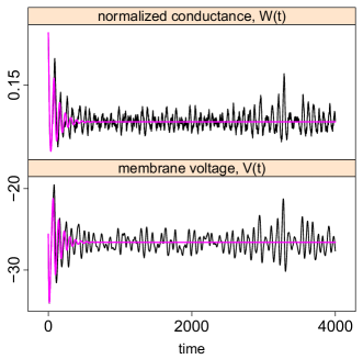
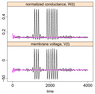
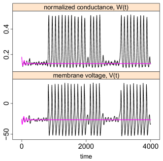
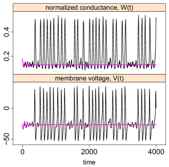
Figure 2: Time series plots (black curves) of the stochastic Morris-Lecar model for different noise levels started inside the unstable limit cycle, but not at the fixed point. Upper left: $\sigma^{*}=0.02$, upper right: $\sigma^{*}=0.03$, lower left: $\sigma^{*}=0.05$, lower right: $\sigma^{*}=0.1$. Note different scales, in the upper left panel there is no firing. The magenta curves are the deterministic model, $\sigma^{*}=0$.

3 The linear approximation of the stochastic Morris-Lecar during quiescence

To identify the process of subthreshold oscillations, i.e. the dynamics close to the stable fixed point between firings, we analyze the linearized system around this point. Consider the system

$$dV_{t} = f(V_{t},W_{t})dt,$$

$$dW_{t} = g(V_{t},W_{t})dt+h(V_{t},W_{t})dB_{t},$$

where the functions $f(\cdot)$, $g(\cdot)$ and $h(\cdot)$ are given by (1), (3)–(5) and (8).

For the chosen parameter values given in Table 1, the deterministic system, obtained for $h(\cdot)=0$, has a unique locally stable equilibrium point $(V_{\text{eq}},W_{\text{eq}})$ given by

$$W_{\text{eq}}(V_{\text{eq}}) = \frac{\alpha(V_{\text{eq}})}{\alpha(V_{\text{eq}})+\beta(V_{\text{eq}})}\,=\,\frac{1}{2}\left(1+\tanh\left(\frac{V_{\text{eq}}-V_{3}}{V_{4}}\right)\right)$$

and $V_{\text{eq}}$ is the solution to the equation $f(V_{\text{eq}},W_{\text{eq}}(V_{\text{eq}}))=0$, which cannot be solved analytically, but can be found numerically. The input current value $I=90\mu$A/cm² is a typical value well inside the range of $I$ where the deterministic dynamics has a stable limit point inside an unstable limit cycle as shown in Fig. 1A. The equilibrium point for $I=90\mu$A/cm² is

$$(V_{\text{eq}},W_{\text{eq}}) = (-26.6\text{ mV },\,0.129).$$

In terms of the centered variables

$$X_{t}^{(1)}\,=\,V_{t}-V_{\text{eq}} X_{t}^{(2)}\,=\,W_{t}-W_{\text{eq}}$$ ,

the system becomes

$$dX_{t}^{(1)} = f\left((X_{t}^{(1)}\!+V_{\text{eq}}),(X_{t}^{(2)}\!+W_{\text{eq}})\right)dt+0\cdot dB_{t}^{(1)}$$ (9)

$$= f^{*}(X_{t}^{(1)},X_{t}^{(2)})dt,$$

$$dX_{t}^{(2)} = g\left((X_{t}^{(1)}\!+V_{\text{eq}}),(X_{t}^{(2)}\!+W_{\text{eq}})\right)dt+h\left((X_{t}^{(1)}\!+V_{\text{eq}}),(X_{t}^{(2)}\!+W_{\text{eq}})\right)dB_{t}^{(2)}\hskip 8.53581pt$$ (10)

$$= g^{*}(X_{t}^{(1)},X_{t}^{(2)})dt+h^{*}(X_{t}^{(1)},X_{t}^{(2)})dB_{t}^{(2)}.$$

We write $X_{t}=(X_{t}^{(1)}\quad X_{t}^{(2)})^{T}$ and $B_{t}=(B_{t}^{(1)}\quad B_{t}^{(2)})^{T}$, where ^T denotes transposition. Note that $B_{t}^{(1)}$ does not enter the dynamics, but is introduced to ease the matrix notation, as will be clear in the following. When the noise is small and the process $X_{t}$ is started near the equilibrium point, $x=(0,0)$, we expect the dynamics to concentrate around the equilibrium point. A local approximation is obtained by linearizing (9)–(10) around $(0,0)$. The diffusion term is approximated by setting $X_{t}^{(1)}=X_{t}^{(2)}=0$ in the diffusion coefficients. The linearized system is

$$dX_{t} = \mathbf{M}X_{t}dt+\mathbf{G}dB_{t},$$ (11)

where

$$\mathbf{M} = \begin{pmatrix}m_{11}&m_{12}\\ m_{21}&m_{22}\end{pmatrix}\,=\,\left.\begin{pmatrix}\frac{\partial f^{*}}{\partial x_{1}}&\frac{\partial f^{*}}{\partial x_{2}}\\ \frac{\partial g^{*}}{\partial x_{1}}&\frac{\partial g^{*}}{\partial x_{2}}\end{pmatrix}\right|_{(x_{1},x_{2})=(0,0)}\!=\,\begin{pmatrix}0.0258&-22.961\\ 0.000335&-0.0446\end{pmatrix},$$

using the parameter values in Table 1, and

$$\mathbf{G} = \begin{pmatrix}0&0\\[5.69054pt] 0&\sigma^{*}\sqrt{2(\alpha(V_{\text{eq}})+\beta(V_{\text{eq}}))}(1-W_{\text{eq}})W_{\text{eq}}\end{pmatrix}\,=\,\begin{pmatrix}0&0\\[5.69054pt] 0&\sigma\end{pmatrix},$$ (12)

where $\sigma=0.034\sigma^{*}$. By evaluating the diffusion approximation of [16] at $(V_{\text{eq}},W_{\text{eq}})$ and equating to the above we obtain $\sigma^{*}=1/\sqrt{W_{\text{eq}}(1-W_{\text{eq}})N}\approx 3/\sqrt{N}$. In the Appendix the matrix $\mathbf{M}$ is detailed. Solutions of (11) with $\mathbf{G}=0$ are given in terms of the eigenvalues of $\mathbf{M}$ which are complex conjugates and given by

$$-\lambda\pm\omega i = -0.0094\pm 0.0803i$$

where $\lambda=-\text{tr}(\mathbf{M})/2$, $\omega^{2}=|\lambda^{2}-\det(\mathbf{M})|$ and $i=\sqrt{-1}$. Thus, near the equilibrium point the solution of (11), with $\sigma=0$, is

$$X_{t} = \mathbf{C}\begin{pmatrix}\cos\omega t\\ \sin\omega t\end{pmatrix}e^{-\lambda t},$$ (13)

where $\mathbf{C}$ contains the initial conditions

$$\mathbf{C} = \begin{pmatrix}x_{0}&(m_{12}y_{0}+(m_{11}+\lambda)x_{0})/\omega\\ y_{0}&(m_{21}x_{0}-(m_{11}+\lambda)y_{0})/\omega\end{pmatrix}.$$

In Fig. 3 the solution of the deterministic model, (1)–(5) with $\sigma=0$, is compared to the linear approximation (13).

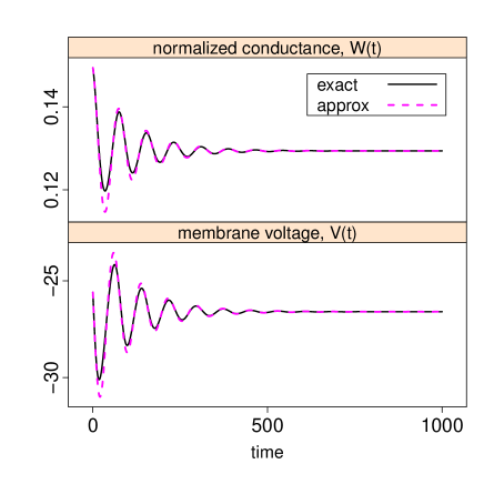
Figure 3: The solution of the deterministic model (1)–(5) with $\sigma=0$ (black full drawn curves) is compared to the linear approximation (13) (cyan dashed curves). Upper panel: normalized conductance $W_{t}$ (dimensionless). Lower panel: membrane potential $V_{t}$ (mV). Time is measured in ms.

4 Identification of the stochastic process of quiescence

In this Section we identify the stochastic process defined by the linearized system (11) in the limit of small $\lambda$, i.e. under the condition $\lambda\ll\omega$. The deterministic system (13) has decaying oscillations, whereas for the stochastic system (11), the noise will prevent the decay of the oscillations. Can we describe the resulting process specifically? The answer is that, after a linear change of variables, this process can be approximated in distribution by a fixed matrix times a deterministic circular motion modulated by an OU process.

We follow the development in [2], where a first step is to transform the matrix $\mathbf{M}$ into a form which reveals the slow decay towards the equilibrium point and the fast oscillatory structure of the deterministic dynamics. Let $\mathbf{Q}$ be a $2\times 2$ matrix such that

$$\mathbf{Q}^{-1}\mathbf{M}\mathbf{Q} = \begin{pmatrix}-\lambda&\omega\\ -\omega&-\lambda\end{pmatrix}\,\doteq\,\mathbf{A}.$$

A possible choice for $\mathbf{Q}$ is

$$\mathbf{Q} = \begin{pmatrix}-\omega&m_{11}+\lambda\\ 0&m_{21}\end{pmatrix}.$$

Let $\tilde{X}_{t}=\mathbf{Q}^{-1}X_{t}$, then

$$d\tilde{X}_{t} = \mathbf{A}\tilde{X}_{t}dt+\mathbf{C}dB_{t}$$ (14)

where $\mathbf{C}=\mathbf{Q}^{-1}\mathbf{G}$. A further change of variables moves the rotation to form part of the diffusion coefficient of the linear stochastic system. We define

$$\tilde{\tilde{X}}_{t} = R_{\omega t}\tilde{X}_{t}$$

where

$$R_{s} = \begin{pmatrix}\cos s&-\sin s\\ \sin s&\cos s\end{pmatrix}$$

is the counterclockwise rotation of angle $s$. Then by Ito’s formula

$$d\tilde{\tilde{X}}_{t} = -\lambda\tilde{\tilde{X}}_{t}dt+R_{\omega t}\mathbf{C}dB_{t}.$$ (15)

The infinitesimal covariance matrix in (14) is

$$\mathbf{B} = \mathbf{C}\mathbf{C}^{T}\,=\,\mathbf{Q}^{-1}\mathbf{G}\mathbf{G}^{T}(\mathbf{Q}^{-1})^{T}\,=\,\frac{\sigma^{2}}{m_{21}^{2}\omega^{2}}\begin{pmatrix}(m_{11}+\lambda)^{2}&\omega(m_{11}+\lambda)\\ \omega(m_{11}+\lambda)&\omega^{2}\end{pmatrix}.$$

Now define

$$\tau^{2} = \frac{1}{2}\mbox{tr}(\mathbf{B})\,=\,\frac{1}{2}(B_{11}+B_{22})\,=\,-\frac{\sigma^{2}m_{12}}{2\omega^{2}m_{21}},$$ (16)

where we have used that $(m_{11}+\lambda)^{2}+\omega^{2}=-m_{12}m_{21}$. Finally, we rescale $\tilde{\tilde{X}}_{t}$ so that we can compare with a standardized two-dimensional OU process. Let

$$U_{t} = \frac{\sqrt{\lambda}}{\tau}\,\tilde{\tilde{X}}_{t/\lambda}.$$

Relation (15) becomes

$$dU_{t} = -U_{t}dt+\frac{1}{\tau}R_{\omega t/\lambda}\mathbf{C}d\tilde{B}_{t}$$ (17)

where $\tilde{B}_{t}=\sqrt{\lambda}B_{t/\lambda}$ is another standard two-dimensional Brownian motion. The following Theorem from [2] allows us to approximate the process $U_{t}$ given by (17), by a two-dimensional OU process with independent coordinates.

Theorem 1.

For each fixed $t^{*}>0$ and $x\in{\rm I\mkern-2.5mu\nonscript\mkern-0.5muR}^{2}$ the distribution of $\{U_{t}:0\leq t\leq t^{*}\}$ given by (17) with $U_{0}=x$ converges as $\lambda/\omega\rightarrow 0$ to the distribution of the standardized two-dimensional OU process $\{S_{t}:0\leq t\leq t^{*}\}$ generated by

$$dS_{t} = -S_{t}dt+dB_{t}$$

with $S_{0}=x$.

Here $S_{t}$ follows a normal distribution, $S_{t}\sim N\left(S_{0}e^{-t},\frac{1}{2}(1-e^{-2t})\mathbf{I}\right)$, where $\mathbf{I}$ is the $2\times 2$ identity matrix. The proof of this Theorem uses a martingale problem convergence argument and involves the notion of stochastic averaging, where fast oscillations integrate out revealing the remaining structure determined by slower oscillations. Another result of this type obtained by a different method, called multiscale analysis, is in [17].

Thus, the process $U_{t}$ is approximated by $S_{t}$ if $\lambda\ll\omega$. In our case $\lambda$ is one order of magnitude smaller than $\omega$.

Putting together the transformations and the final approximation we have, in the sense of stochastic process distributions,

$$X_{t} = \mathbf{Q}\tilde{X}_{t}\,=\,\mathbf{Q}R_{-\omega t}\tilde{\tilde{X}}_{t}\,=\,\mathbf{Q}R_{-\omega t}\frac{\tau}{\sqrt{\lambda}}\,U_{\lambda t}\,\approx\,\mathbf{Q}R_{-\omega t}\frac{\tau}{\sqrt{\lambda}}\,S_{\lambda t}$$ (18)

$$= \frac{\tau}{\sqrt{\lambda}}\begin{pmatrix}-\omega&m_{11}+\lambda\\ 0&m_{21}\end{pmatrix}\begin{pmatrix}\cos\omega t&\sin\omega t\\ -\sin\omega t&\cos\omega t\end{pmatrix}S_{\lambda t}.$$

Let us denote by $X_{t}^{a}$ the stochastic process on the right hand side of (18), i.e.

$$X_{t}^{a} = \tau\mathbf{Q}R_{-\omega t}\,S_{\lambda t}/\sqrt{\lambda}.$$ (19)

To get a sense of how closely the process $X_{t}^{a}$ approximates the dynamics of the ML process in a neighborhood of $(V_{\text{eq}},W_{\text{eq}})$ we compare their power spectral densities, as well as that of the solution of the linearized system (11). The spectral density of $X_{t}^{a}$ and that of$X_{t}$ satisfying (11) can be calculated explicitly using the power spectrum formula of [10] for linear diffusions of the form (11). In fact $X_{t}^{a}$ is such a diffusion: the effect of the stochastic averaging can be seen as replacing $\mathbf{C}$ from (14) by a multiple of the identity in the system (14), so the approximation to $\tilde{X}$ satisfies $d\tilde{X}^{a}_{t}=\mathbf{A}\tilde{X}^{a}_{t}dt+\tau dB_{t}$, where $\tau$ is given by (16). If we transform this equation by $X_{t}^{a}=\mathbf{Q}\tilde{X}^{a}_{t}$, we see that $X_{t}^{a}$ satisfies

$$dX^{a}_{t} = \mathbf{M}X^{a}_{t}dt+\tau\mathbf{Q}dB_{t}.$$ (20)

The spectral density of the first coordinate of $X^{a}$ is

$$S(f) = \frac{1}{2\pi}\frac{\sigma^{2}m_{12}^{2}}{\left((f^{2}-\mbox{det}(\mathbf{M}))^{2}+(f\mbox{tr}(\mathbf{M}))^{2}\right)}\frac{\left(f^{2}+\mbox{det}(\mathbf{M})\right)}{2\omega^{2}},$$

whereas the spectral density of the first coordinate of the linearized system, (11), is

$$S(f) = \frac{1}{2\pi}\frac{\sigma^{2}m_{12}^{2}}{(f^{2}-\mbox{det}(\mathbf{M}))^{2}+(f\mbox{tr}(\mathbf{M}))^{2}}.$$

In Fig. 4 the theoretical spectral densities for the two approximations are plotted, together with the estimated spectral density of the quiescent process from simulations of the stochastic ML model (1),(3)–(5) and (8). The spectral density is estimated by averaging over at least 20 estimates from paths started at 0 of at least 450 ms of subthreshold fluctuations, and scaled to have the same maximum as the theoretical spectral density from (20). The averaging is done to reduce the large variance connected with spectral density estimation, avoiding any smoothing. Thus, the estimator is approximately unbiased, see also [8] where this approach is treated. The estimation is done for $\sigma^{*}=0.03,0.05$ and 0.1. For higher noise, the lengths of subthreshold fluctuations between spikes are too short to reliably estimate the spectral density. Moreover, $\sigma^{*}=0.1$ corresponds to a number of ion channels $N\approx 900$, which can be considered a minimum acceptable number for the diffusion approximation to be relevant. The value $\sigma^{*}=0.03$ corresponds to $N\approx 10,000$. Remember that $\sigma=0.034\sigma^{*}$, see (12).

The approximations are only acceptable for small noise, which is expected, since larger noise brings the process to areas further away from the fixed point, where non-linearities become increasingly important.

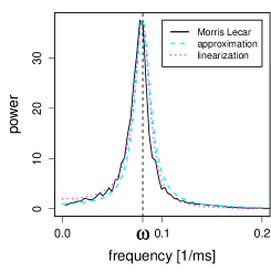
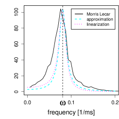
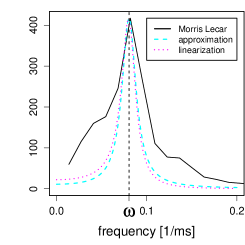
Figure 4: Spectral density estimated from simulations between spikes of model (1), (3)–(5), (8) (black solid line), theoretical spectral density of model (20) (cyan dashed line), and theoretical spectral density of model (11) (magenta dotted line). From left to right: $\sigma^{*}=0.03,0.05$ and $0.1$.

5 Reconstructing the stochastic ML firing mechanism

In this Section we construct a firing mechanism matching that of the stochastic ML neuron. In Section 6 we will define a new LIF-type process by combining this firing mechanism with the radial OU process. This new model will, for small $\sigma$, have an ISI distribution similar to that of the ML.

Firing in model (1), (3)–(5) and (8) occurs when the stochastic dynamics shifts from a path circulating the stable equilibrium, modulated by an OU, to a noisy circuiting of the stable limit cycle. This shift happens, roughly, when the orbit passes from the inside to the outside of the unstable limit cycle. When the orbit comes close to the unstable limit cycle, it will follow this limit cycle for a short time, and then escape either to the inside, i.e. continue its subthreshold oscillations, or to the outside and a spike will occur. This understanding is not accurate enough to be implemented as a firing scheme for the radial OU process (27), as we discuss further in Section 7. Hence, we embed the process $X^{a}$ defined by (19) in the stochastic ML model by constructing a firing mechanism mimicking that of the ML itself. It is clear that in the ML model, starting inside the unstable limit cycle, a spike will occur with increasing probability, the further away the process is from the fixed point. In order to construct a firing mechanism matching that of ML, we will estimate, from simulations, the conditional probability that the ML fires, given that the trajectory of the ML crosses the line $L=\{(v,w):v=V_{\mbox{eq}},w<W_{\mbox{eq}}\}$. We computed estimates from simulated data using crossings of the line $L$ as follows.

For a given value of $\sigma^{*}$ and distance $l$ from the fixed point, a short trajectory starting in $(V_{\mbox{eq}},W_{\mbox{eq}}-l)$ was simulated from model (1), (3)–(5) and (8), and it was registered whether firing occurred in the first cycle of the stochastic path around $(V_{\mbox{eq}},W_{\mbox{eq}})$. Firing was defined by the path crossing the line $v=0$, which is well above the largest level inside the unstable limit cycle, see Fig. 1B. This was repeated $1000$ times, and estimates of the conditional probability of spiking, $\hat{p}(l,\sigma^{*})$, were computed as the frequency of the trajectories where firing occurred. The procedure was repeated for $l=l_{i}=i\delta,i=1,\ldots,25$, where $\delta$ is the distance to the stable limit cycle divided by 20. In this way a grid of possible $l$ values was covered, starting from $l=0$ at the fixed point, where the probability of firing is close to zero, to a point on $L$ below the stable limit cycle, where the probability of firing is close to one. The estimation was, furthermore, repeated for $\sigma^{*}=0.01$ to $0.08$ in steps of $0.01$.

For each fixed $\sigma^{*}$, the estimates of the conditional probability appear to depend in a sigmoidal way on the distance from the fixed point. We assumed the conditional firing probability to be of the form

$$p(l) = \frac{1}{1+\exp((\alpha-l)/\beta)}.$$ (21)

  

Figure 5: Conditional probability of spiking when crossing the line $L=\{(v,w):v=V_{\mbox{eq}},w<W_{\mbox{eq}}\}$ for different values of $\sigma^{*}$. (A) Original space. The circles, plus’s and stars are individual nonparametric estimates obtained using $\sigma^{*}=0.02,0.05$ and 0.08, respectively, with the fitted curves on top given by (21). The dashed line indicates where the unstable limit cycle crosses $L$, the full drawn line where the stable limit cycle crosses $L$. (B) The fitted curves in the transformed space for $\sigma^{*}=0.02,0.03,0.04,0.05,0.06,0.07$ and $0.08$ (right to left), as a function of the distance from the fixed point in the transformed coordinates. The crosses and boxed crosses indicate the crossing of the unstable and stable limit cycles of $L$, respectively, which depend on $\sigma=0.034\sigma^{*}$.

$\sigma^{*}$	0.01	0.02	0.03	0.04	0.05	0.06	0.07	0.08
$\hat{\alpha}$	0.0174	0.0174	0.0169	0.0168	0.0171	0.0169	0.0167	0.0168
$\hat{\beta}$	0.0006	0.0013	0.0020	0.0028	0.0033	0.0039	0.0047	0.0054
$\hat{\alpha}\sqrt{2\lambda}/\sigma$	7.1022	3.5426	2.3012	1.7156	1.3922	1.1474	0.9739	0.8549
$\hat{\beta}\sqrt{2\lambda}/\sigma$	0.2590	0.2624	0.2759	0.2831	0.2718	0.2674	0.2738	0.2764

Table 2: Estimates of regression parameters for $p(\cdot)$ in the original space (first two rows), and in the transformed coordinates (last two rows).

The parameters $\alpha$ and $\beta$ were estimated using non-linear regression of the 25 estimates of $\hat{p}(l_{i};\sigma^{*})$ on $l$. In Fig. 5A these parametric estimates are plotted, as well as the individual nonparametric estimates $\hat{p}$ for $\sigma^{*}=0.02,0.05$ and $0.08$. We see that the family of estimates, $\hat{p}$, fits the hypothetic curve quite well for each value of $\sigma^{*}$. Regression estimates are reported in Table 2. Note that $\alpha$ is the distance along $L$ from $W_{\mbox{eq}}$ at which the conditional probability of firing equals one half. For all values of $\sigma^{*}$, the estimate of $\alpha$ is close to the distance along $L$ between $W_{\mbox{eq}}$ and the unstable limit cycle, which equals 0.0172. In other words, the probability of firing, if the path starts at the intersection of $L$ with the unstable limit cycle, is about 1/2. The parameter $\beta$ indicates the width of a band around $\alpha$ where the conditional probability essentially changes. For instance, if $l\in\alpha\pm\beta$ then $p(l)\in(0.27,0.73)$, if $l\in\alpha\pm 2\beta$ then $p(l)\in(0.12,0.88)$. As expected, the estimate of $\beta$ increases with increasing $\sigma^{*}$, and for small noise the conditional probability approaches a step function since the process is mostly dominated by the drift. A step function would correspond to the firing being represented by a first-passage time of a fixed threshold. Note though that $\hat{\beta}$ is approximately proportional to $\sigma^{*}$, and thus, as we said earlier and will see in the following, a fixed threshold at the crossing of the unstable limit cycle does not reproduce the desired spiking characteristics.

In order to simplify the construction in Section 6 of a LIF model which, together with a firing rule, behaves like the stochastic ML, we will change coordinates as follows. Observe that (19) can be written

$$\frac{\sqrt{\lambda}}{\tau}\mathbf{Q}^{-1}X_{t}^{a} = \begin{pmatrix}\cos\omega t&\sin\omega t\\ -\sin\omega t&\cos\omega t\end{pmatrix}S_{\lambda t},$$ (22)

so for fixed $t$, $\sqrt{\lambda}\mathbf{Q}^{-1}X_{t}^{a}/\tau$ is the clockwise rotation by angle $\omega t$ of the orthogonal pair $(S_{\lambda t}^{(1)},S_{\lambda t}^{(2)})$. We define a transformation of the space $(v,w)$ by centering at $(V_{\mbox{eq}},W_{\mbox{eq}})$ and normalizing as in (22). Let

$$\begin{pmatrix}\tilde{v}\\ \tilde{w}\end{pmatrix} = \frac{\sqrt{\lambda}}{\tau}\mathbf{Q}^{-1}\begin{pmatrix}v-V_{\text{eq}}\\ w-W_{\text{eq}}\end{pmatrix}$$ (23)

be the coordinates of the transformed space. In the new coordinates our process is simplified to a rotation modulated by a standard two-dimensional OU process with independent components.

The transformation depends on $\sigma=0.034\sigma^{*}$, namely, the transformed unstable limit cycle becomes smaller with increasing noise, through the value of $\tau$ given in (16). This is exactly what is causing a higher firing probability for larger $\sigma^{*}$. The line $L$ will in the transformed space be

$$\tilde{L} = \frac{\sqrt{\lambda}}{\tau}\mathbf{Q}^{-1}\begin{pmatrix}0\\ l\end{pmatrix}=\frac{\sqrt{\lambda}}{m_{21}\tau}\begin{pmatrix}\frac{m_{11}+\lambda}{\omega}\\ 1\end{pmatrix}l$$

for $l\geq 0$. A distance $l$ will thus transform to a distance $r=(\sqrt{2\lambda}/\sigma)l$, and the conditional probability of firing (21) transforms to

$$p(r) = \frac{1}{1+\exp((\alpha^{*}-r)/\beta^{*})},$$ (24)

where $\alpha^{*}=\alpha\sqrt{2\lambda}/\sigma$ and $\beta^{*}=\beta\sqrt{2\lambda}/\sigma$. The fitted curves of (24) for $\sigma^{*}=0.02-0.08$, as a function of the distance from the fixed point in the transformed coordinates are given in Fig. 5B, with indication of the crossings of the unstable and stable limit cycles, respectively, which now depend on $\sigma$. Note that in the transformed space, the width of the band where the conditional probability is essentially different from 0 or 1 is nearly constant, see Table 2. From here on we use the coordinates defined by (23).

6 Construction of a leaky-integrate-and-fire model with ML firing statistics

The simpler stochastic LIF models sacrifice realism for mathematical tractability [4, 11]. In these models, a neuron is characterized by a single stochastic differential equation describing the evolution of neuronal membrane potential depending on time,

$$dX_{t} = \mu(X_{t})dt+\sigma(X_{t})dB_{t},\quad\quad X_{0}=x_{0},$$ (25)

where $X_{t}$ corresponds to $V_{t}$ in the ML model, together with a threshold firing rule,

$$T = \inf\{t>0:X_{t}\geq S\}.$$ (26)

In this Section we define a LIF model which does not make this compromise, using the result of Section 4 and the firing mechanism defined in Section 5.

The distance of the approximate process $\sqrt{\lambda}\mathbf{Q}^{-1}X_{t}^{a}/\tau$ of (22) from the point $(0,0)$ at time $t$ is given by the modulus of the two-dimensional standardized OU process $S_{\lambda t}$. The modulus of $S_{\lambda t}$ at time $t$ is given by the process

$$R_{\lambda t} = \sqrt{(S_{\lambda t}^{(1)})^{2}+(S_{\lambda t}^{(2)})^{2}},$$

which is a standard radial OU process with two degrees of freedom. It has state space $(0,\infty)$, and solves the stochastic differential equation

$$dR_{\lambda t} = \left(\frac{1}{2R_{\lambda t}}-R_{\lambda t}\right)dt+dW_{\lambda t},$$ (27)

see e.g. [3]. We define a new LIF process by (27), and firing mechanism derived from (24). After each firing, we will reset the time to 0 and assume the process reset to 0, i.e. $R_{0}=0$, corresponding to $S_{0}=(0,0)$ and $(V_{0},W_{0})=(V_{\mbox{eq}},W_{\mbox{eq}})$. By Ito’s formula, the process $Y_{u}=R_{u}^{2}$ satisfies the stochastic differential equation

$$dY_{u} = 2\left(1-Y_{u}\right)du+2\sqrt{Y_{u}}dW_{u},$$ (28)

and is thus a square-root process, see e.g. [5], also called a Feller or a Cox-Ingersoll-Ross process. This process is ergodic, and its stationary distribution is the exponential distribution with mean one. It follows that the stationary distribution of $R_{u}$ has density $f(r)=2re^{-r^{2}}$ on $(0,\infty)$, i.e. it follows a Rayleigh distribution. The transition density of $Y_{u}$ starting at $y_{0}$ at time 0, is a non-central $\chi^{2}$-distribution with two degrees of freedom and non-centrality parameter $\delta(u,y_{0})=2y_{0}e^{-2u}/(1-e^{-2u})$. Then $2Y_{u}/(1-e^{-2u})$ follows the standard non-central $\chi^{2}$-distribution $F_{\chi^{2}}(2y/(1-e^{-2u}),2,\delta(u,y_{0}))$. It is particularly simple because of the integer degrees of freedom. Transforming to the radial OU we obtain the transition density of $R_{u}$ starting at $s$ at time 0

$$f_{u}(r,s) = \frac{2r}{1-e^{-2u}}\exp\left\{-\frac{r^{2}+s^{2}e^{-2u}}{1-e^{-2u}}\right\}I_{0}\left(\frac{rs}{\sinh(u)}\right),$$ (29)

where $I_{0}(x)=\frac{1}{\pi}\int_{0}^{\pi}e^{x\cos\theta}d\theta$ is the modified Bessel function of the first kind of index 0.

Writing the two-dimensional process $S_{u}$ in polar coordinates, $R_{u}$ and $\theta_{u}$, where $\theta_{u}$ is the angle at time $u$ to the positive part of the first coordinate, we find that the modulus and the angle are independent, and that $\theta_{u}$ is uniformly distributed on $(0,2\pi)$. This can e.g. be seen from the fact that $S_{u}^{(1)}$ and $S_{u}^{(2)}$ are independent normal with mean 0 and equal variances. Thus, for fixed $u$, $S_{u}^{(2)}/S_{u}^{(1)}$ is standard Cauchy distributed and $\theta_{u}=\arctan(S_{u}^{(2)}/S_{u}^{(1)})$ is $U(0,2\pi)$.

Let $T$ denote the firing time random variable. We want to compute the density of the distribution of $T$, and for this we find it convenient to express this density in terms of the conditional hazard rate,

$$\alpha(t,r) = \lim_{\Delta t\rightarrow 0}\frac{1}{\Delta t}P(t\leq T<t+\Delta t\,|\,T\geq t,R_{\lambda t}=r).$$

This function is the density of the conditional probability, given the position on $L$ is $r$ at time $t$, of a spike occuring in the next small time interval, given that it has not yet occurred.

From standard results from survival analysis, see e.g. [1], we obtain

$$P(T>t\,|\,R_{\lambda s},0\leq s\leq t) = \exp\left(-\int_{0}^{t}\alpha(R_{\lambda s})ds\right).$$

The unconditional distribution is then given by

$$P(T>t) = E\left(\exp\left(-\int_{0}^{t}\alpha(R_{\lambda s})ds\right)\right)$$ (30)

where $E(\cdot)$ denotes expectation with respect to the distribution of $R$. The density is thus

$$g(t)\,=\,\frac{d}{dt}P(T\leq t) = E\left(\alpha(R_{\lambda t})\exp\left(-\int_{0}^{t}\alpha(R_{\lambda s})ds\right)\right).$$ (31)

The firing is defined to be initiated from $L$, and on average the process crosses $L$ every $2\pi/\omega=78.2$ time units. Using (24), the estimated conditional probability of firing given the position on $L$ is $r$, which by definition does not depend on $t$, we estimate the hazard rate as

$$\alpha(t,r)\,=\,\alpha(r) = \frac{\omega}{2\pi}\frac{1}{1+\exp((\alpha^{*}-r)/\beta^{*})}.$$ (32)

Note that it is bounded. This is not realistic, since a very large value of $r$ should cause immediate firing.

In [21] a firing rule with unbounded hazard rate was proposed, and in [15] it was shown to fit well to experimental data. Therefore, we will also see how our model performs if we use in the firing mechanism a hazard rate of the form

$$\alpha(t,r)\,=\,\alpha(r) = \exp((r-\alpha)/\beta)$$ (33)

for $\alpha,\beta>0$. Like before, $\alpha$ plays the role of a threshold, and $\beta$ gives the width of the threshold region. When $\beta\rightarrow 0$, the firing rule converges to a fixed threshold crossing. To estimate $\alpha$ and $\beta$ in (33), we simulated 1000 spike times from the ML. The cumulative hazard $A(t)=\int_{0}^{t}\alpha(t)$ was then estimated from the simulated spike times by the standard empirical Nelson-Aalen estimator. The theoretical cumulative hazard using (27) and (33) can be calculated as

$$A(t) = E\left(\int_{0}^{t}\alpha(R_{\lambda s})ds\right)\,=\,\exp\left(-\frac{\alpha}{\beta}\right)\int_{0}^{t}E\left(\exp\left(\frac{R_{\lambda s}}{\beta}\right)\right)ds$$ (34)

$$= \sqrt{\pi}\exp\left(-\frac{\alpha}{\beta}\right)\int_{0}^{t}\left(g(s)\exp\left(\frac{1}{4}g(s)^{2}\right)\Phi\left(g(s)\right)+1\right)ds$$

where we have used the density $f_{\lambda s}(r,0)$ given in (29). Here, $g(s)=\sqrt{1-e^{-2\lambda s}}/\beta$, and $\Phi(\cdot)$ is the standard normal cumulative distribution function. Then, $\alpha$ and $\beta$ were estimated by the least square distance between (34) and the estimated cumulative hazard from the simulated spike times. For $\sigma^{*}=0.05$ the estimates were $\alpha=6.31$ and $\beta=0.76$.

The final model is

$$dR_{u} = \left(\frac{1}{2R_{u}}-R_{u}\right)dt+dW_{u}-R_{u-}\mu(R_{u-},du),$$ (35)

where $\mu(R_{u-},du)$ is a Poisson measure with intensity $\alpha(R_{u-})$, and $R_{u-}$ denotes the left limit of $R_{u}$. Here, $\alpha(\cdot)$ is either given by (32) or (33). The jump size is $-R_{u-}$, thus giving the reset to 0 at spike times.

A reasonable alternative to the soft threshold firing mechanism used here would be to use the firing rule defined by a threshold as in the classical LIF models, equation (26). A natural choice of threshold would be where the LIF process reaches a level corresponding to the unstable limit cycle. In fact, according to our estimates in Fig. 5 and Table 2, the firing probability of the ML at this threshold is around $1/2$. However, the ISI distribution estimated from simulations using a hard threshold at the unstable limit cycle is shifted towards larger times, relative to the ML ISI distribution. This happens because the process might cycle many times inside the unstable limit cycle, so even if the probability of spiking in a single cycle is small, the total probability is not negligible. This is lost when only a hard threshold is considered. Instead we chose the threshold value such that the mean of the ML ISI distribution and the mean of the LIF ISI distribution were the same. In [12], the mean of $T$ from (26) with $X_{t}=R_{t}$ started at $R_{0}=0$ is given using a hypergeometric function,

$$E(T) = \frac{S^{2}}{2}\,_{2}F_{2}\left(1,1;2,2;S^{2}\right).$$ (36)

The average of the 1000 ML firing times for $\sigma^{*}=0.05$ was 447. Equating with (36) gives a value $S=2.97$ for the hard threshold. Note that this is much smaller than the estimated $\alpha$ from (33).

7 Comparison of firing statistics

One of the major issues in computational neuroscience is to determine the ISI distribution. We therefore simulated the ML model given by (1), (3)–(5) and (8) until spiking, and thereafter reset to the fixed point. This was done 1000 times, and the time of the firing was recorded. The ISI distribution from our approximate model is given by the density (31), or equivalently, from the survival function (30). Due to the law of large numbers and since we know the exact distribution of $R_{u}$, for fixed $t$ we can numerically determine (31) up to any desired precision by choosing $n$ and $M$ large enough through the expression

$$g(t) \approx \frac{1}{M}\sum_{m=1}^{M}\alpha\left(R_{\lambda t}^{(m)}\right)\exp\left(-\frac{t}{n}\sum_{i=1}^{n}\frac{\alpha\left(R_{i\lambda t/n}^{(m)}\right)+\alpha\left(R_{(i-1)\lambda t/n}^{(m)}\right)}{2}\right).$$ (37)

Here $(R_{0}^{(m)},\ldots,R_{i\lambda t/n}^{(m)},\ldots,R_{\lambda t}^{(m)})$ are $M$ realizations of $R_{i\lambda t/n}$, $i=0,1,\ldots,n$, and the integral has been approximated by the trapezoidal rule. The hazard rate is either given by (32) or (33).

The results are illustrated in Figure 6 for $\sigma^{*}=0.05$, using $M=1000$. The estimated ISI distributions from our approximate model with both firing mechanisms compare well with the estimated ISI distribution of ML reset to 0 after firings. On the contrary, the hard threshold does not reproduce the ISI distribution well, e.g. the right tail is too heavy. This is because the probability of firing during low subthreshold activity is set to 0, whereas we have seen it is not.

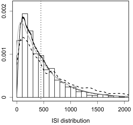
Figure 6: Distribution of firing times for $\sigma^{*}=0.05$. The histogram is based on 1000 simulated firing times from the ML model, the vertical dotted line is the average. Curves are estimates of the probability density, equation (37). Black curve is estimated using (32), gray curve is estimated using (33), dashed curve is estimated using a fixed threshold, (26).

8 Discussion

A stochastic LIF model constructed with a radial OU process and firing mechanism of either logistic or exponential type has been shown to mimic the ISI statistics of a ML neuron model. It captures subthreshold dynamics, not of the membrane potential alone, but of a combination of the membrane potential and ion channels. This construction will allow us to answer several questions about ML models, which have been accessible only for LIF models, even though the latter have less biological motivation.

An example of such a question would be: Using ISI experimental data, the noise standard deviation $\sigma$ can be estimated [18]. In principle, this should also be possible from our new LIF model, even though we use a soft threshold. This will give an estimate of $N$, the number of ion channels involved, through the relation $(\sigma^{*})^{2}\approx 9/N$.

A question we have not explored is: what is the best way to restart our new LIF model? In our simulations we restarted both our LIF and the ML at the fixed point of the ML. However, an uninterrupted stochastic ML produces continuous paths as in Fig. 1B. After firing, which means traversing the large stable limit cycle, possibly several times, they reenter a neighborhood of the fixed point from its edge. A further refinement of our LIF model will be obtained by introducing a reentry mechanism, which mimics this aspect of the ML.

Appendix A Linearization matrix

The expression for $\mathbf{M}$ in (11) is

$$\mathbf{M} = \begin{pmatrix}m_{11}&-g_{k}W_{\text{eq}}(V_{\text{eq}}-V_{K})/C\\[5.69054pt] 2V_{\text{eq}}W_{\text{eq}}\beta\left(V_{\text{eq}}\right)/V_{4}&-\alpha\left(V_{\text{eq}}\right)\end{pmatrix},$$

$$m_{11} = -\frac{V_{\text{eq}}}{C}\left(\frac{2g_{\text{Ca}}(V_{\text{eq}}-V_{\text{Ca}})\alpha\left(V_{\text{eq}}\right)\beta\left(V_{\text{eq}}\right)}{V_{2}(\alpha\left(V_{\text{eq}}\right)+\beta\left(V_{\text{eq}}\right))^{2}}+g_{\text{Ca}}m_{\infty}(V_{\text{eq}})+g_{K}W_{\text{eq}}+g_{L}\right)$$

S. Ditlevsen supported by the Danish Council for Independent Research$\,|\,$Natural Sciences. P. Greenwood supported by the Statistical and Applied Mathematical Sciences Institute, Research Triangle Park, N.C., and the Mathematical, Computational and Modeling Sciences Center at Arizona State University. The Villum Kann Rasmussen foundation supported a 4 months visiting professorship for P. Greenwood at University of Copenhagen.

References

- [1] Aalen, O. O., Borgan, Ø. and Gjessing, H. K. (2010). Survival and Event History Analysis. A process point of view. Springer, New York.
- [2] Baxendale, P. and Greenwood, P. (2011). Sustained oscillations for density dependent Markov processes. J. Math. Biol. To appear, available online.
- [3] Borodin, A. N. and Salminen, P. (2002). Handbook of Brownian motion - Facts and Formulae. Probability and its applications. Birkhauser Verlag, Basel.
- [4] Burkitt, A. N. (2006). A review of the integrate-and-fire neuron model: I. homogeneous synaptic input. Biol. Cybern. 95, 1–19.
- [5] Cox, J. C., Ingersoll, J. E. and Ross, S. A. (1985). A theory of the term structure of interest rates. Econometrica 53, 385–407.
- [6] Dayan, P. and Abbott, L. F. (2001). Theoretical Neuroscience: Computational and Mathematical Modeling of Neural Systems. MIT Press, Cambridge.
- [7] Ditlevsen, S. and Jacobsen, M. (2011). Ergodic solutions to multidimensional diffusions. In preparation.
- [8] Ditlevsen, S., Yip, K.-P. and Holstein-Rathlou, N.-H. (2005). Parameter estimation in a stochastic model of the tubuloglomerular feedback mechanism in a rat nephron. Mathematical Biosciences 194, 49–69.
- [9] Forman, J. L. and Sørensen, M. (2008). The Pearson diffusions: A class of statistically tractable diffusion processes. Scand. J. Stat. 35, 438–465.
- [10] Gardiner, C. W. (1990). Handbook of stochastic methods for physics, chemistry and the natural sciences 2nd ed. Springer, Berlin Heidelberg.
- [11] Gerstner, W. and Kistler, W. M. (2002). Spiking Neuron Models. Cambridge Uni. Press, Cambridge.
- [12] Graczyk, P. and Jakubowski, T. (2008). Exit times and Poisson kernels of the Ornstein-Uhlenbeck diffusion. Stochastic Models 24, 314–337.
- [13] Hodgkin, A. L. and Huxley, A. F. (1952). A quantitative description of ion currents and its applications to conduction and excitation in nerve membranes. J. Physiol. 117, 500–544.
- [14] Izhikevich, E. M. (2007). Dynamical systems in neuroscience: the geometry of excitability and bursting. MIT Press, Cambridge.
- [15] Jahn, P., Berg, R. W., Hounsgaard, J. and Ditlevsen, S. (2011). Motoneuron membrane potentials follow a time inhomogeneous jump diffusion process. J. Comput. Neurosci. To appear, available online.
- [16] Kurtz, T. G. (1978). Strong approximation theorems for density dependent Markov chains. Stoch. Proc. Appl. 6, 223–240.
- [17] Kuske, R., Gordillo, L. F. and Greenwood, P. (2007). Sustained oscillations via coherence resonance in SIR. J. Theor. Biol. 245, 459–469.
- [18] Lansky, P. and Ditlevsen, S. (2008). A review of the methods for signal estimation in stochastic diffusion leaky integrate-and-fire neuronal models. Biol. Cybern. 99, 253–262.
- [19] Lapicque, L. (1907). Recherches quantitatives sur l’excitation electrique des nerfs traitee comme une polarization. J. Physiol. Pathol. Gen. 9, 620–35.
- [20] Morris, C. and Lecar, H. (1981). Voltage oscillations in the barnacle giant muscle fiber. Biophysics Journal 35, 193–213.
- [21] Pfister, J. P., Toyoizumi, T., Barber, D. and Gerstner, W. (2006). Optimal spike-timing-dependent plasticity for precise action potential firing in supervised learning. Neural Comput. 18, 1318–1348.
- [22] Rinzel, J. and Ermentrout, B. (1998). In: Methods in neuronal modeling 2nd ed. MIT Press, Cambridge. ch. Analysis of neural excitability and oscillations, pp. 251–291.
- [23] Tateno, T. and Pakdaman, K. (2004). Random dynamics of the Morris-Lecar neural model. Chaos 14, 511–530.