Black-hole horizons as probes of black-hole dynamics II: geometrical insights

Abstract

In a companion paper Jaramillo et al. (2012), we have presented a cross-correlation approach to near-horizon physics in which bulk dynamics is probed through the correlation of quantities defined at inner and outer spacetime hypersurfaces acting as test screens. More specifically, dynamical horizons provide appropriate inner screens in a $3+1$ setting and, in this context, we have shown that an effective-curvature vector measured at the common horizon produced in a head-on collision merger can be correlated with the flux of linear Bondi-momentum at null infinity. In this paper we provide a more sound geometric basis to this picture. First, we show that a rigidity property of dynamical horizons, namely foliation uniqueness, leads to a preferred class of null tetrads and Weyl scalars on these hypersurfaces. Second, we identify a heuristic horizon newslike function, depending only on the geometry of spatial sections of the horizon. Fluxes constructed from this function offer refined geometric quantities to be correlated with Bondi fluxes at infinity, as well as a contact with the discussion of quasilocal 4-momentum on dynamical horizons. Third, we highlight the importance of tracking the internal horizon dual to the apparent horizon in spatial 3-slices when integrating fluxes along the horizon. Finally, we discuss the link between the dissipation of the nonstationary part of the horizon’s geometry with the viscous-fluid analogy for black holes, introducing a geometric prescription for a “slowness parameter” in black-hole recoil dynamics.

I Introduction

In Ref. Jaramillo et al. (2012) (paper I hereafter) a cross-correlation methodology for studying near-horizon strong-field physics was outlined. Spacetime dynamics was probed through the cross-correlation of timeseries $h_{\mathrm{inn}}$ and $h_{\mathrm{out}}$ defined as geometric quantities on inner and outer hypersurfaces, respectively. The latter are understood as test screens whose geometries respond to the bulk dynamics, so that the (global) functional structure of the constructed cross-correlations encodes some of the features of the bulk geometry. This is in the spirit of reconstructing spacetime dynamics in an inverse-scattering picture. In the context of asymptotically flat black-hole (BH) spacetimes, the BH event horizon ${E}$ and future null infinity ${I}^{+}$ provide natural test hypersurfaces from a global perspective. However, when a $3+1$ approach is adopted for the numerical construction of the spacetime, dynamical trapping horizons ${\cal H}$ provide more appropriate hypersurfaces to act as inner test screens. In the application of this correlation strategy to the study of BH post-merger recoil dynamics, an effective-curvature vector $\tilde{K}^{\mathrm{eff}}_{i}(v)$ was constructed Jaramillo et al. (2012) on ${\cal H}$ as the quantity $h_{\mathrm{inn}}$ to be cross-correlated with $h_{\mathrm{out}}$, where the latter is the flux of Bondi linear momentum $(dP_{i}^{\mathrm{B}}/du)(u)$ at ${I}^{+}$ (here, $u$ and $v$ denote, respectively, advanced and retarded times). In this paper we explore some geometric structures underlying and extending the heuristic construction in Jaramillo et al. (2012) of this effective local probe into BH recoil dynamics.

The adaptation of geometric structures and tools from ${I}^{+}$ to BH horizons is at the basis of important geometric developments in BH studies, notably the quasilocal frameworks of isolated and dynamical trapping horizons Hayward (1994a); Ashtekar and Krishnan (2003, 2004) (see also Refs. Hayward (1994b, 2003)). In this spirit, the construction of $\tilde{K}^{\mathrm{eff}}_{i}(v)$ on the horizon ${\cal H}$ partially mimics the functional structure of the flux of Bondi linear momentum at ${I}^{+}$. In particular, $(dP_{i}^{\mathrm{B}}/du)(u)$ can be expressed in terms of (the dipolar part of) the square of the news function ${\cal N}$ on sections of ${I}^{+}$, whereas the definition of $\tilde{K}^{\mathrm{eff}}_{i}(v)$ involves the (dipolar part of the) square of a function $\tilde{\cal N}$ constructed from the Ricci scalar ${}^{2}\!R$ on sections of ${\cal H}$. However, the functions ${\cal N}$ and $\tilde{\cal N}$ differ in their spin-weight and, more importantly, they show a different behavior in time: whereas ${\cal N}(u)$ is an object well-defined in terms of geometric quantities on time sections ${\cal S}_{u}\subset{{I}^{+}}$, nothing guarantees this local-in-time character of $\tilde{\cal N}(v)$ [see Eq. (4) below]. The latter is a crucial characteristic of the news function, so that $\tilde{\cal N}(v)$ cannot be considered as a valid newslike function on ${\cal H}$.

These structural differences suggest that, in spite of the success of $\tilde{K}^{\mathrm{eff}}_{i}$ in capturing effectively (at the horizon) some qualitative aspects of the flux of Bondi linear momentum (at null infinity), a deeper geometric insight into the dynamics of ${\mathcal{H}}$ can provide hints for a refined correlation treatment. In this context, the specific goals in this paper are: i) to justify the role of $\tilde{K}^{\mathrm{eff}}_{i}$ as an effective quantity to be correlated to $(dP_{i}^{\mathrm{B}}/du)$, suggesting candidates offering a refined version; ii) to explore the introduction of a valid newslike function on ${\cal H}$, only depending on the geometry of sections ${\cal S}_{v}\subset{\cal H}$; iii) to establish a link between the cross-correlation approach in Jaramillo et al. (2012) and other approaches to the study of the BH recoil based on quasilocal momentum.

The paper is organized as follows. Section II introduces the basic elements on the inner screen ${\cal H}$ geometry and revisits the effective-curvature vector of paper I. Aiming at understanding the dynamics of the latter, a geometric system governing the evolution of the intrinsic curvature along the horizon ${\cal H}$ is discussed, making apparent the key driving role of the Weyl tensor. In Sec. III some fundamental results on dynamical horizons are discussed, in particular a rigidity structure enabling a preferred choice of null tetrad on ${\cal H}$. Proper contractions of the latter with the Weyl tensor lead in Sec. IV to newslike functions and associated Bondi-like fluxes on ${\cal H}$ providing refined quantities on the horizon to be correlated with Bondi fluxes at ${I}^{+}$, as well as making contact with quasilocal approaches to BH linear momentum. In Sec. V our geometric discussion is related to the viscous-fluid analogy of BH horizons, providing in particular a geometric prescription for the slowness parameter $P$ in Price et al. (2011). Conclusions are presented in Sec. VI. Finally a first appendix gathers the geometric notions in the text, whereas a second appendix emphasizes the physical relevance of internal horizons when computing fluxes along ${\cal H}$. We use a spacetime signature $(-,+,+,+)$, with abstract index notation (first letters, $a$, $b$, $c$…, in Latin alphabet) and Latin midalphabet indices, $i,j,k...$, for spacelike vectors. We also employ the standard convention for the summation over repeated indices. All the quantities are expressed in a system of units in which $c=G=1$.

II Geometric evolution system on the horizon: the role of the Weyl tensor

II.1 The inner screen ${\cal H}$

Let us consider a BH spacetime $({\cal M},g_{ab})$, with associated Levi-Civita connection $\nabla_{a}$, endowed with a $3+1$ spacelike foliation $\{\Sigma_{t}\}$. Let us consider an inner hypersurface ${\cal H}$, to be later identified with the BH horizon, such that the intersection of the slices $\Sigma_{t}$ with the world-tube ${\cal H}$ defines the foliation of ${\cal H}$ by closed spacelike surfaces $\{{\cal S}_{t}\}$. We consider an evolution vector $h^{a}$ along ${\cal H}$, characterized as that vector tangent to ${\cal H}$ and normal to the slices $\{{\cal S}_{t}\}$ that transports the slice ${\cal S}_{t}$ onto the slice ${\cal S}_{t+\delta t}$. The normal plane at each point of ${\cal S}_{t}$ can be spanned in terms of the outgoing null vector $\ell^{a}$ and the ingoing vector $k^{a}$, chosen to satisfy $\ell^{a}k_{a}=-1$. Directions of $\ell^{a}$ and $k^{a}$ are fixed, though a rescaling freedom remains (see Fig.1). In particular, and without loss of generality in our context, we can write Booth and Fairhurst (2004)

$$h^{a}=\ell^{a}-Ck^{a},$$ (1)

so that $h^{a}h_{a}=2C$. Therefore: $h^{a}$ is, respectively, spacelike if $C>0$, null if $C=0$, and timelike if $C<0$.

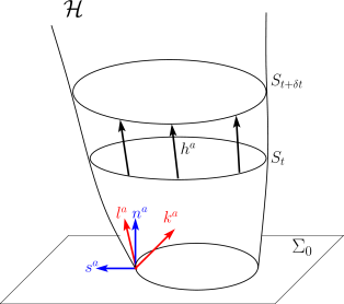
Figure 1: Worldtube ${\cal H}$ foliated by closed spacelike surfaces $\{{\cal S}_{t}\}$ as the result of a $3+1$ spacelike foliation $\{\Sigma_{t}\}$. The evolution vector $h^{a}$ (tangent to ${\cal H}$ and normal to $\{{\cal S}_{t}\}$) transports the slice ${\cal S}_{t}$ to ${\cal S}_{t+\delta t}$. The normal plane at each point of ${\cal S}_{t}$ can be spanned by the outgoing and ingoing null normal vectors $\ell^{a}$ and $k^{a}$ or by $n^{a}$, the unit timelike normal to $\Sigma_{t}$, and $s^{a}$, the spacelike outgoing normal to $S_{t}$ and tangent to $\Sigma_{t}$ (cf. Appendix A) .

Regarding the intrinsic geometry on ${\cal S}_{t}$, the induced metric is denoted by $q_{ab}$, its Levi-Civita connection by ${}^{2}\!D_{a}$ and the corresponding Ricci curvature scalar by ${}^{2}\!R$. The area form is ${}^{2}\!\epsilon=\sqrt{q}dx^{1}\wedge dx^{2}$ and we will denote the area measure as $dA=\sqrt{q}d^{2}x$. The infinitesimal evolution of the intrinsic geometry along ${\cal H}$, i.e., the evolution of the induced geometry $q_{ab}$ along $h^{a}$, defines the deformation tensor $\Theta^{(h)}_{ab}$ [cf. Equation (50) in Appendix A]

$$\Theta^{(h)}_{ab}\equiv\frac{1}{2}{\delta}_{h}q_{ab}=\sigma^{(h)}_{ab}+\frac{1}{2}\theta^{(h)}q_{ab}\,,$$ (2)

where the trace $\theta^{(h)}=\Theta^{(h)}_{ab}q^{ab}$, referred to as the expansion along $h^{a}$, measures the infinitesimal evolution of the ${\cal S}_{t}$ element of area along ${\cal H}$, whereas the traceless shear $\sigma^{(h)}_{ab}$ controls the deformations of the induced metric (see Eq. (53) in Appendix A). Here $\delta_{h}$ can be identified with the projection on ${\cal H}$ of the Lie derivative ${\cal L}_{h}$ [see Eq. (49) and the remark after Eq. (56)]. Before reviewing the effective-curvature vector $\tilde{K}^{\mathrm{eff}}_{i}$, let us discuss the time parametrization of ${\cal H}$.

We recall that jumps of apparent horizons (AHs) are generic in $3+1$ evolutions of BH spacetimes. The dynamical trapping horizon framework offers a spacetime insight into this behavior by understanding the jumps as corresponding to marginally trapped sections of a (single) hypersurface bending in spacetime, but multiply foliated by spatial hypersurfaces in the $3+1$ foliation $\{\Sigma_{t}\}$ Booth et al. (2006); Nielsen and Visser (2006); Schnetter et al. (2006); Booth and Fairhurst (2008); Jaramillo et al. (2009). In the particular case of binary BH mergers this picture predicts, after the moment of its first appearance, the splitting of the common AH into two horizons: a growing external common horizon and a shrinking internal common horizon Schnetter et al. (2006); Jaramillo et al. (2009). It is standard to track the evolution of the external common horizon, the proper AH, but to regard the internal common horizon as physically irrelevant. In Appendix B we stress however the relevance of the internal horizon in the context of the calculation of physical fluxes into the black-hole singularity.

In Fig. 2 we illustrate this picture in a simplified (spherically symmetric) collapse scenario that retains the relevant features of the discussion. On one side, the relevant outer screen boundary (namely, null infinity ${I}^{+}$) is parametrized by the retarded time $u$, something explicitly employed in the expression of the flux of Bondi momentum in Eqs. (33) and (34) of paper I. On the other side, from the $3+1$ perspective, the moment $t_{c}$ of first appearance of the (common) horizon corresponds to the coordinate time $t$ at which the $3+1$ foliation $\{\Sigma_{t}\}$ firstly intersects the dynamical horizon ${\cal H}$. For $t>t_{c}$, $\Sigma_{t}$ slices intersect twice (multiply, in the generic case) the hypersurface ${\cal H}$ giving rise to the external and internal common horizons (cf. ${\cal H}$ in Fig. 2). Therefore, the time function $t$ is not a good parameter for the whole dynamical horizon ${\cal H}$. An appropriate parametrization of this hypersurface ${\cal H}$ is given in terms of an advanced time, such as $v$, parametrizing past null infinity ${I}^{-}$. More precisely, (for a spacelike world-tube portion of ${\cal H}$) we can label sections of ${\cal H}$ by an advanced time $v$ starting from an initial value $v_{0}$ corresponding to the first $v=\mathrm{const}$ null hypersurface hitting the spacetime singularity, i.e., ${\cal H}=\bigcup_{v\geq v_{0}}{\cal S}_{v}$.

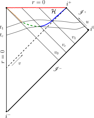
Figure 2: Carter-Penrose diagram (corresponding, for simplicity, to a generic spherically symmetric collapse) illustrating the time parametrization of the outer and inner screens. The outer boundary given by ${I}^{+}$ is properly parametrized by the retarded time $u$, whereas an advanced time $v$ runs along inner boundaries, in particular the dynamical horizon ${\cal H}$. Given a $3+1$ foliation $\{\Sigma_{t}\}$, $t_{c}$ denotes the time $t$ at which the horizon first appears. For $t>t_{c}$, $\Sigma_{t}$ slices intersect multiply the hypersurface ${\cal H}$, giving rise to internal and external horizons. On the contrary, the advanced coordinate $v$ provides a good parametrization of ${\cal H}$ from an initial $v>v_{0}$.

II.2 Effective-curvature vector $\tilde{K}^{\mathrm{eff}}_{i}$

In paper I the effective-curvature vector $\tilde{K}^{\mathrm{eff}}_{i}$ was introduced using the parametrization of ${\cal H}$ by the time function $t$ associated with the spacetime $3+1$ slicing. In particular, $\tilde{K}^{\mathrm{eff}}_{i}(t)$ was defined only on the external part of the horizon ${\cal H}$, for $t\geq t_{c}$. We can now extend the definition of $\tilde{K}^{\mathrm{eff}}_{i}$ to the whole horizon ${\cal H}$ (more precisely, to a spacelike world-tube portion of it) by making use of its parametrization by the advanced time $v$ adapted to the $3+1$ slicing of ${\cal H}$. Given a section ${\cal S}_{v}\subset{\cal H}$, we consider a vector $\xi^{i}$ transverse to it (i.e., generically not tangent to ${\cal S}_{v}$) and tangent to the 3-slice $\Sigma_{t}$ that intersects ${\cal H}$ at ${\cal S}_{v}$ (i.e., ${\cal S}_{v}={\cal H}\cap\Sigma_{t}$). Then, the component $\tilde{K}^{\mathrm{eff}}[\xi](v)$ is expressed as

$$\tilde{K}^{\mathrm{eff}}[\xi](v)\propto-\oint_{{\cal S}_{v}}(\xi^{i}s_{i})\left(\tilde{\cal N}(v)\right)^{2}dA\,,$$ (3)

where $s_{i}$ is the spacelike normal to ${\cal S}_{v}$ and tangent to $\Sigma_{t}$, and

$$\tilde{\cal N}(v)\equiv\int_{v_{0}}^{v}{}^{2}\!R(v^{\prime})dv^{\prime}+\tilde{\cal N}_{v_{0}}\,,$$ (4)

where ${}^{2}\!R$ is the Ricci curvature scalar on $({\cal S}_{v},q_{ab})$ and $\tilde{\cal N}_{v_{0}}$ is an initial function to be fixed. As commented above, in spite of the formal similarity with the news function ${\cal N}(u)$ at ${I}^{+}$ [cf. Equation (34) in paper I), definition (4] does not guarantee the local-in-time character of $\tilde{\cal N}(v)$ since it is expressed in terms of a time integral on the past history.

In order to study the dynamics of $\tilde{K}^{\mathrm{eff}}_{i}$, we consider the evolution of the Ricci scalar curvature ${}^{2}\!R$ along the world-tube ${\cal H}$ . In terms of the elements introduced above, the evolution of the Ricci scalar curvature ${}^{2}\!R$ along $h^{a}$ has the form

$$\delta_{h}{}^{2}\!R=-\theta^{(h)}\,{}^{2}\!R+2\;{}^{2}\!D^{a}{}^{2}\!D^{b}\sigma^{(h)}_{ab}-{}^{2}\!\Delta\theta^{(h)}\ \,,$$ (5)

where ${}^{2}\!\Delta=q^{ab}{}^{2}\!D_{a}{}^{2}\!D_{b}$ denotes the Laplacian on ${\cal S}_{t}$. Expression (5) is a fundamental one in our work and it applies to any hypersurface ${\cal H}$ foliated by closed surfaces ${\cal S}_{t}$. Contact with BHs is made when ${\cal H}$ is taken as the spacetime event horizon or as the dynamical horizon associated with the foliation $\{\Sigma_{t}\}$.

II.3 Geometry evolution on BH horizons

We briefly recall the notions of BH horizon relevant here and refer to Appendix A for a systematic presentation of the notation. First, the event horizon (EH) ${E}$ is the boundary of the spacetime region from which no signal can be sent to ${I}^{+}$, i.e., the region in ${\cal M}$ not contained in the causal past $J^{-}({I}^{+})$ of ${I}^{+}$. The EH is a null hypersurface, characterized as ${E}=\partial J^{-}({I}^{+})\cap{\cal M}$. Second, a dynamical horizon (DH) or (dynamical) future outer trapping horizon ${\cal H}$ is a quasilocal model for the BH horizon based on the notion of a world-tube of AHs. More specifically, a future outer trapping horizon ${\cal H}$ is a hypersurface that can be foliated by marginally (outer) trapped surfaces ${\cal S}_{t}$, i.e., ${\cal H}=\bigcup_{t\in\mathbb{R}}{\cal S}_{t}$ with outgoing expansion $\theta^{(\ell)}=0$ on ${\cal S}_{t}$, satisfying: i) a future condition $\theta^{(k)}<0$, and ii) an outer condition $\delta_{k}\theta^{(\ell)}<0$. In the dynamical regime, i.e., when matter and/or radiation cross the horizon (namely when $\delta_{\ell}\theta^{(\ell)}\neq 0$), the outer condition is equivalent to the condition that ${\cal H}$ is spacelike Booth and Fairhurst (2007). Therefore, for dynamical trapping horizons we have $C>0$ in Eq. (1) [cf. discussion after Eq. (59)].

For both EHs and DHs, an important area theorem holds: $\delta_{h}A=\oint_{{\cal S}_{t}}\theta^{(h)}dA>0$. In the case of an EH, Hawking’s area theorem Hawking (1971, 1972) guarantees the growth of the area, whereas in the case of a DH, the positivity of $\delta_{h}A=-\oint_{{\cal S}_{t}}C\theta^{(k)}dA$ [cf. Equation A.2] is guaranteed by its spacelike character ($C>0$) together with the future condition $\theta^{(k)}<0$.

We make now contact with Eq. (5) and interpret the elements that determine the dynamics of ${}^{2}\!R$. The growth of the area of a BH horizon guarantees the (average) positivity of $\theta^{(h)}$. This offers a qualitative understanding of the dynamical decay of ${}^{2}\!R$: the first term in the right-hand side drives an exponential-like decay of the Ricci scalar curvature. More precisely, nonequilibrium deformations of the Ricci scalar curvature ${}^{2}\!R$ in BH horizons decay exponentially as long as the horizon grows in area. Regarding the elliptic operators acting on the shear and the expansion [second and third terms in the right hand side of Eq. (5)] they provide dissipative terms smoothing the evolution of ${}^{2}\!R$. Indeed, in Sec. V we will review a viscosity interpretation of $\theta^{(h)}$ and $\sigma^{(h)}_{ab}$, in particular associating with them respective decay and oscillation timescales of the horizon geometry.

II.3.1 Complete evolution system driving ${}^{2}\!R$

A further understanding of Eq. (5) requires a control of the dynamics of the shear $\sigma^{(h)}_{ab}$, of the expansion $\theta^{(h)}$ and of the induced metric $q_{ab}$, the latter controlling the elliptic operators ${}^{2}\!D^{a}{}^{2}\!D^{b}$ and ${}^{2}\!\Delta$. Therefore, we need evolution equations determining $\delta_{h}q_{ab}$, $\delta_{h}\theta^{(h)}$ and $\delta_{h}\sigma^{(h)}_{ab}$:

i) $\delta_{h}q_{ab}$: definition of the deformation tensor. The evolution of $q_{ab}$ is dictated by $\sigma^{(h)}_{ab}$ and $\theta^{(h)}$ [cf. Equation (2)].

ii) $\delta_{h}\theta^{(h)}$: focusing or Raychadhuri-like equation. The evolution of $\theta^{(h)}$ involves the Ricci tensor $R_{ab}$, i.e., the “trace part” of the spacetime Riemann tensor ${R^{a}}_{bcd}$, thus introducing the stress-energy tensor $T_{ab}$ through Einstein equations.

iii) $\delta_{h}\sigma^{(h)}_{ab}$: tidal equation. The evolution of $\sigma^{(h)}_{ab}$ is driven by the Weyl tensor ${C^{a}}_{bcd}$, i.e., the traceless part of the spacetime Riemann tensor, thus involving dynamical gravitational degrees of freedom but not directly the Einstein equations.

The structural feature that we want to underline about these equations is shared by evolution systems on EHs and DHs, although the explicit form of the equations differ in both cases. More specifically, whereas for EHs the evolution equations for ${}^{2}\!R$, $q_{ab}$, $\theta^{(h)}$ and $\sigma^{(h)}_{ab}$ form a “closed” evolution system, in the DH case additional geometric objects (requiring further evolution equations) are brought about through the evolution equations $\delta_{h}q_{ab}$, $\delta_{h}\theta^{(h)}$ and $\delta_{h}\sigma^{(h)}_{ab}$. Moreover, an explicit dependence on the function $C$, related to the choice of $3+1$ slicing as discussed later [cf. Equation (III)], is involved in the DH case. For these reasons, and for simplicity, in the rest of this subsection we restrict our discussion to the case of an EH, indicating that the main qualitative conclusion also holds for DHs, whose details will be addressed elsewhere.

The EH ${E}$ is a null hypersurface generated by the evolution vector $h^{a}$, a null vector in this case: $h^{a}=\ell^{a}$. The null generator $\ell^{a}$ satisfies a pregeodesic equation $\ell^{c}\nabla_{c}\ell^{a}=\kappa^{(\ell)}\ell^{a}$ [see Eq. (56) for the expression of the nonaffinity parameter $\kappa^{(\ell)}$]. Choosing an affine reparametrization such that $\ell^{a}$ is geodesic, i.e., $\kappa^{(\ell)}=0$, the evolution equations for ${}^{2}\!R$, $q_{ab}$, $\sigma^{(h)}_{ab}$ and $\theta^{(h)}$ close the evolution system

$$\delta_{\ell}{}^{2}\!R = -\theta^{(\ell)}\,{}^{2}\!R+2\;{}^{2}\!D^{a}{}^{2}\!D^{b}\sigma^{(\ell)}_{ab}-{}^{2}\!\Delta\theta^{(\ell)}\,,$$ (6)

$$\delta_{\ell}q_{ab} = 2\sigma^{(\ell)}_{ab}+\theta^{(\ell)}q_{ab}\,,$$ (7)

$$\delta_{\ell}\theta^{(\ell)} = -\frac{1}{2}(\theta^{(\ell)})^{2}-\sigma^{(\ell)}_{ab}{\sigma^{(\ell)}}^{ab}-8\pi T_{ab}\ell^{a}\ell^{b}\,,$$ (8)

$$\delta_{\ell}\sigma^{(\ell)}_{ab} = \sigma^{(\ell)}_{cd}{\sigma^{(\ell)}}^{cd}q_{ab}-{q^{c}}_{a}{q^{d}}_{b}C_{lcfd}\ell^{l}\ell^{f}\,.$$ (9)

Once initial conditions are prescribed, the only remaining information needed to close the system are the matter term $T_{ab}\ell^{a}\ell^{b}$ in the focusing equation and ${q^{c}}_{a}{q^{d}}_{b}C_{lcfd}\ell^{l}\ell^{f}$ in the tidal equation. Using a null tetrad $(\ell^{a},k^{a},m^{a},\overline{m}^{a})$ (see Appendix A) they can be expressed in terms of Ricci and Weyl scalars: $8\pi T_{ab}\ell^{a}\ell^{b}=R_{ab}\ell^{a}\ell^{b}=2\Phi_{00}$ and ${q^{c}}_{a}{q^{d}}_{b}C_{lcfd}\ell^{l}\ell^{f}=\Psi_{0}\overline{m}_{a}\overline{m}_{b}+\overline{\Psi}_{0}m_{a}m_{b}$. The complex Weyl scalar $\Psi_{0}$ and the Ricci scalar $\Phi_{00}$ drive the evolution of the geometric system (6)–(9) on the horizon. Being determined in terms of the bulk dynamics ($\Psi_{0}$ relates to the near-horizon dynamical tidal fields and incoming gravitational radiation, whereas $\Phi_{00}$ accounts for the matter fields), fields $\Psi_{0}$ and $\Phi_{00}$ act as external forces providing (modulo initial conditions) all the relevant dynamical information for system (6)–(9) on ${E}$.

In the DH case, although the evolution system is more complex, the qualitative conclusions reached here remain unchanged. More specifically, the differential system on ${\cal H}$ governing the evolution of ${}^{2}\!R$ is also driven by external forces given by a particular combination of Weyl and Ricci scalars.

In the present cross-correlation approach, these dynamical considerations strongly support $\Psi_{0}$ as a natural building block in the construction of the quantity $h_{\mathrm{inn}}(v)$ at ${\cal H}$, to be correlated in vacuum to $dP_{i}^{\mathrm{B}}/du$ at ${I}^{+}$. This is hardly surprising, given the dual nature of $\Psi_{0}$ and $\Psi_{4}$ on inner and outer boundaries, respectively.

Particularly relevant are the following remarks. First, in the presence of matter, the scalar $\Phi_{00}$ plays a role formally analogous to that of $\Psi_{0}$. Therefore, in the general case, it makes sense to consider $\Phi_{00}$ on an equal footing as $\Psi_{0}$ in the construction of $h_{\mathrm{inn}}(v)$. Second, Eq. (6) is completely driven by the rest of the system, without back-reacting on it. For this reason, although $\Psi_{0}$ (and $\Phi_{00}$) encodes the information determining the dynamics on the horizon, at the same time the evolution of ${}^{2}\!R$ is sensitive to all relevant dynamical degrees of freedom, providing an averaged response. This justifies the crucial role of ${}^{2}\!R$ in the construction of the effective $\tilde{K}_{i}^{\mathrm{eff}}$ in paper I.

A serious drawback for the use of $\Psi_{0}$ and $\Phi_{00}$ in the construction of a quantity $h_{\mathrm{inn}}(v)$ at ${\cal H}$ is their dependence on the rescaling freedom of the null normal $\ell^{a}$ by an arbitrary function on ${\cal S}$. We address this point in the following section.

III Fundamental results on Dynamical Horizons

The introduction of a preferred null tetrad on the horizon requires some kind of rigid structure. We argue here that DHs provide such a structure. We first review two fundamental geometric results about DHs:

a) Result 1 (DH foliation uniqueness) Ashtekar and Galloway (2005): Given a DH ${\cal H}$, the foliation ${\{\cal S}_{t}\}$ by marginally trapped surfaces is unique.

b) Result 2 (DH existence) Andersson et al. (2005, 2008): Given a strictly stably outermost marginally trapped surface ${\cal S}_{0}$ in a Cauchy hypersurface $\Sigma_{0}$, for each $3+1$ spacetime foliation $\{\Sigma_{t}\}$ containing $\Sigma_{0}$ there exists a unique DH ${\cal H}$ containing ${\cal S}_{0}$ and sliced by marginally trapped surfaces $\{{\cal S}_{t}\}$ such that ${\cal S}_{t}\subset\Sigma_{t}$.

These results have the following important implications:

i) The evolution vector $h^{a}$ is completely fixed on a DH (up to time reparametrization). By Result 1 any other evolution vector $h^{\prime a}$ does not transport marginally trapped surfaces into marginally trapped surfaces.

ii) The evolution of an AH into a DH is nonunique. Let us consider an initial AH ${\cal S}_{0}\subset\Sigma_{0}$ and two different $3+1$ slicings $\{\Sigma_{t_{1}}\}$ and $\{\Sigma_{t_{2}}\}$, compatible with $\Sigma_{0}$. From Result 2 there exist DHs ${\cal H}_{1}=\bigcup_{t_{1}}{\cal S}_{t_{1}}$ and ${\cal H}_{2}=\bigcup_{t_{2}}{\cal S}_{t_{2}}$, with ${\cal S}_{t_{1}}={\cal H}_{1}\cap\Sigma_{t_{1}}$ and ${\cal S}_{t_{2}}={\cal H}_{2}\cap\Sigma_{t_{2}}$ marginally trapped surfaces. Let us consider now the sections of ${\cal H}_{1}$ by $\{\Sigma_{t_{2}}\}$, i.e., ${\cal S}^{\prime}_{t_{2}}={\cal H}_{1}\cap\Sigma_{t_{2}}$, so that ${\cal H}_{1}=\bigcup_{t_{2}}{\cal S}^{\prime}_{t_{2}}$. In the generic case, slicings $\{{\cal S}^{\prime}_{t_{2}}\}$ and $\{{\cal S}_{t_{1}}\}$ of ${\cal H}_{1}$ are different (deform $\{\Sigma_{t_{2}}\}$ if needed). Therefore, from Result 1, ${\cal S}^{\prime}_{t_{2}}$ cannot be marginally trapped surfaces. Reasoning by contradiction, we then conclude that ${\cal H}_{1}$ and ${\cal H}_{2}$ are different hypersurfaces in ${\cal M}$, as illustrated in Fig.3.

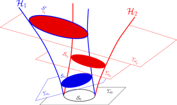
Figure 3: Worldtubes ${\cal H}_{1}$ (blue) and ${\cal H}_{2}$ (red), respectively, associated with two different $3+1$ slicing $\{\Sigma_{t_{1}}\}$ and $\{\Sigma_{t_{2}}\}$ and providing evolutions from a given marginally trapped surface ${\cal S}_{0}$ in an initial Cauchy hypersurface $\Sigma_{0}$. They illustrate the nonunique evolution of AHs into DHs. The foliation $\{{\cal S}_{t_{1}}\}$ (resp. $\{{\cal S}_{t_{2}}\}$ ) by marginally trapped surfaces is defined by the intersections of ${\cal H}_{1}$ with $\{\Sigma_{t_{1}}\}$ (resp. ${\cal H}_{2}$ and $\{\Sigma_{t_{2}}\}$). Note that, from the DH foliation uniqueness Result $1$ Ashtekar and Galloway (2005), surfaces ${\cal S}^{\prime}_{t_{2}}={\cal H}_{1}\cap\Sigma_{t_{2}}$ are not (in general) marginally trapped surfaces.

The two results above establish a fundamental link between DHs and the $3+1$ approach here adopted. We denote (cf. also Appendix A) the unit timelike normal to slices $\Sigma_{t}$ by $n^{a}$ and the spacelike (outgoing) normal to ${\cal S}_{t}$ and tangent to $\Sigma_{t}$ by $s^{a}$ (see Fig.1). We denote by $N$ the lapse associated to the spacetime slicing function $t$, i.e., $n_{a}=-N\nabla_{a}t$. Given a marginal trapped surface ${\cal S}_{0}$ in an initial slice $\Sigma_{0}$, and given a lapse function $N$, let us consider the (only) DH ${\cal H}$ given by Result 2. Then the unique evolution vector $h^{a}$ on ${\cal H}$ associated with Result 1 can be written up to a time-dependent rescaling as

$$h^{a}=Nn^{a}+bs^{a}\ \,,$$ (10)

where $b$ is a function on ${\cal S}_{t}$ to be determined in terms of $N$ and $C$ [see Eq. (III) below]. Certainly such a decomposition of an evolution vector compatible with a given $3+1$ slicing $\{\Sigma_{t}\}$, in the sense $h^{a}\nabla_{a}t=1$, is valid for any hypersurface but, in the case of a DH and due to Result 1, the evolution vector $h^{a}$ determined by Eq. (10) has an intrinsic meaning (up to time reparametrization, which is irrelevant in a cross-correlation approach) as an object on ${\cal H}$ not requiring a $3+1$ foliation. On the other hand, Eq. (1) provides the expression of vector $h^{a}$ in terms of the null normals. More specifically, Eq. (1) links the scaling of $\ell^{a}$ and $k^{a}$ to that of $h^{a}$ by imposing $h^{a}\to\ell^{a}$ as the DH is driven to stationarity ($C\to 0\Leftrightarrow\delta_{\ell}\theta^{(\ell)}\to 0$). Writing the null normals at ${\cal H}$ as $\ell^{a}=(f/2)(n^{a}+s^{a})$ and $k^{a}=(n^{a}-s^{a})/f$, for some function $f$, expressions (1) and (10) for $h^{a}$ lead to

$$\ell_{N}^{a}=\frac{N+b}{2}\left(n^{a}+s^{a}\right)\,,\ k_{N}^{a}=\frac{1}{N+b}\left(n^{a}-s^{a}\right)\,,$$ (11)

where the subindex $N$ denotes the explicit link of ${\cal H}$ to a $3+1$ slicing. In order to determine $b$, we evaluate the norm of $h^{a}$ and note that the function $C$ in Eq. (1) is expressed in terms of $N$ and $b$ as

$$C=\frac{1}{2}\left(b^{2}-N^{2}\right)\ \,.$$ (12)

On the other hand, for a given lapse $N$, the trapping horizon $\delta_{h}\theta^{(\ell)}=0$ condition translates into an elliptic equation for $C$ [cf. Equation (59)]

$$-{}^{2}\!\Delta C+2\Omega^{(\ell)}_{c}{}^{2}\!D^{c}C-C\left[-{}^{2}\!D^{c}\Omega^{(\ell)}_{c}+\Omega^{(\ell)}_{c}{\Omega^{(\ell)}}^{c}-\frac{1}{2}{}^{2}\!R\right]$$

$$=\sigma^{(\ell)}_{ab}{\sigma^{(\ell)}}^{ab}+8\pi T_{ab}\tau^{a}\ell^{b}\,.$$ (13)

Therefore, for a given DH ${\cal H}$ associated with a $3+1$ slicing with lapse $N$, Eqs. (III) and (12) fix the value of $b$. Prescription (11) provides then preferred null normals on a DH ${\cal H}$ compatible with the foliation defined by $N$. Completed with the complex null vector $m^{a}$ on ${\cal S}_{t}$, we propose

$$(\ell^{a}_{N},k^{a}_{N},m^{a},\overline{m}^{a})\ ,$$ (14)

as a preferred null tetrad (up to time reparametrization) on a DH. To keep the notation compact, hereafter we will denote the preferred $\ell^{a}_{N}$ and $k^{a}_{N}$ simply as $\ell^{a}$ and $k^{a}$ and omit the symbol $N$ from all quantities evaluated in this tetrad. The tetrad (14) then leads to a notion of preferred Weyl (and Ricci) scalars on the horizon ${\cal H}$. In particular,

$$\Psi_{0} = C^{a}_{\ \,bcd}\;\ell_{a}m^{b}\ell^{c}m^{d}\,,$$ (15)

$$\Phi_{00} = \frac{1}{2}R_{ab}\;\ell^{a}\ell^{b}\,.$$ (16)

In summary: we have introduced preferred null normals on a DH ${\cal H}$ by: i) linking the normalization of $\ell^{a}$ to that of $h^{a}$ by requiring $h^{a}\to\ell^{a}$ in stationarity; and ii) fixing the normalization of $h^{a}$ (up to a time-dependent function) by the foliation uniqueness result on DHs (Result 1). The latter is the rigid structure needed to fix a preferred null tetrad on ${\cal H}$. In the particular case of constructing ${\cal H}$ in an initial value problem approach (Result 2 on DHs), the free time-dependent function is fixed by the lapse $N$ of the given global foliation $\{\Sigma_{t}\}$.

IV News-like functions and Bondi-like fluxes on a dynamical horizon

IV.1 News-like functions: vacuum case

In Sec. II we have identified the Weyl scalar $\Psi_{0}$ as the object that encodes (in vacuum and for $C=0$) the relevant geometric information on the BH horizon understood as an inner screen. Then in Sec. III we have introduced a preferred scaling for $\Psi_{0}$ on DHs. With these elements we can now introduce the following vectorial quantity on ${\cal H}$

$$\tilde{K}[\xi](v)\equiv-\frac{1}{8\pi}\oint_{{\cal S}_{v}}(\xi^{i}s_{i})\left|\tilde{\cal N}_{\Psi}^{(\ell)}(v)\right|^{2}dA\,,$$ (17)

with

$$\tilde{\cal N}_{\Psi}^{(\ell)}(v)\equiv\int_{v_{0}}^{v}\Psi_{0}(v^{\prime})dv^{\prime}\,,$$ (18)

where we make use of an advanced time $v$ parametrizing ${\cal H}$ (cf. Sec. II.1 and Fig. 2) and adapted to the $3+1$ slicing at ${\cal H}$ (namely, we choose $h^{a}\nabla_{a}v=2$ to match the general notation in paper I).

The quantity $\tilde{K}_{i}$ could be used as a refined version of $\tilde{K}^{\mathrm{eff}}_{i}$ for the correlation with $dP_{i}^{\mathrm{B}}/du$ at ${I}^{+}$. However, whereas $\tilde{K}^{\mathrm{eff}}_{i}$ is explicitly understood as an effective quantity and, consequently, one can relax the requirement on the $\tilde{\cal N}$ constructed out of ${}^{2}\!R$ in (4) to behave mathematically as a news function, the situation is different for $\tilde{K}_{i}$ in (17): the geometric dual nature of $\Psi_{4}$ and $\Psi_{0}$ would call for a newslike function character for $\tilde{\cal N}^{(\ell)}_{\Psi}$ in (18).

Whereas expressions for the flux of Bondi momentum and the news function at ${I}^{+}$ [cf. Equations (33) and (34) in paper I] are valid under the (strong) conditions enforced by asymptotic simplicity at null infinity and in a given Bondi frame, no geometric structure supports the “a priori” introduction of quantities $\tilde{K}_{i}$ and $\tilde{\cal N}^{(\ell)}_{\Psi}$ on ${\cal H}$. In particular, the news function ${\cal N}(u)$ is an object well-defined in terms of geometric quantities on sections ${\cal S}_{u}\subset{I}^{+}$, that can be expressed as a time integral [cf. Eq. (34) in paper I] due to the key relation $\partial_{u}{{\cal N}}=\Psi_{4}$ holding for Bondi coordinate systems at ${I}^{+}$. On the contrary, the quantity $\tilde{\cal N}^{(\ell)}_{\Psi}$ defined by time integration of $\Psi_{0}$ is not an object defined in terms of the geometry of a section ${\cal S}_{v}$ (justifying the use of a “tilde”). Such a local-in-time behavior is a crucial property to be satisfied by any valid news function. Therefore, one would expect additional terms to $\Psi_{0}$ (with vanishing counterparts at ${I}^{+}$), contributing in $\tilde{\cal N}^{(\ell)}_{\Psi}$ to build an appropriate newslike function on ${\cal H}$.

In the absence of a sound geometric news formalism on ${\cal H}$, we proceed heuristically by modifying $\tilde{\cal N}^{(\ell)}_{\Psi}$ so that it acquires a local-in-time character. Such a property would be guaranteed if the integrand in definition (18) could be expressed as a total derivative in time of some quantity defined on sections ${\cal S}_{v}$. The scalar $\Psi_{0}$ in Eq. (18) does not satisfy this property. However, with this guideline, inspection of (9) suggests some of the terms to be added to $\Psi_{0}$ [system (6)–(9) applies to the EH case] so that they integrate in time to a quantity on ${\cal S}_{v}$, namely the shear. Considering first, as an intermediate step, the EH case and using a tensorial rather a complex notation, let us introduce a newslike tensor $({\cal N}^{(\ell)}_{\Psi})_{ab}$ whose time variation is

$$(\dot{\cal N}^{(\ell)}_{\Psi})_{ab}=\frac{1}{\sqrt{2}}\left({q^{c}}_{a}{q^{d}}_{b}C_{lcfd}\ell^{l}\ell^{f}-\sigma^{(\ell)}_{cd}{\sigma^{(\ell)}}^{cd}q_{ab}\right)\,,$$ (19)

that is, such that $(\dot{\cal N}^{(\ell)}_{\Psi})_{ab}=-1/\sqrt{2}\delta_{\ell}\sigma^{(\ell)}_{ab}$ (the global factor $1/\sqrt{2}$ is required for the correct coefficient in the leading-order contribution). Upon time integration in Eq. (18) and setting vanishing initial values at early times, this choice leads to

$$({\cal N}^{(\ell)}_{\Psi})_{ab}=-\frac{1}{\sqrt{2}}\sigma^{(\ell)}_{ab}\ \ \,.\ \ \$$ (20)

If we write

$$({\cal N}^{(\ell)}_{\Psi})_{ab} = \frac{1}{\sqrt{2}}\int_{v_{0}}^{v}\left[{q^{c}}_{a}{q^{d}}_{b}C_{lcfd}\ell^{l}\ell^{f}-\right.$$ (21)

$$\left.2({\cal N}^{(\ell)}_{\Psi})_{cd}({{\cal N}^{(\ell)}}_{\Psi})^{cd}q_{ab}\right]dv^{\prime}\,,$$

and substitute $({\cal N}^{(\ell)}_{\Psi})_{ab}$ recursively in the right hand side, we can express the newslike function $({\cal N}^{(\ell)}_{\Psi})_{ab}$ in terms of $\Psi_{0}$ so that the lowest-order term is indeed given by expression (18).

This identification, in the EH case, of a plausible newslike tensor as the shear along the evolution vector suggests the following specific proposal for the newslike tensor for DHs

$${\cal N}^{{}^{({\cal H})}}_{ab}\equiv-\frac{1}{\sqrt{2}}\sigma^{(h)}_{ab}\,.$$ (22)

This proposal has a tentative character. Once we have identified the basics, we postpone a systematic study to a forthcoming work.

IV.2 News-like functions: matter fields

As discussed in Sec. II, in system (6)–(9) the Ricci scalar $\Phi_{00}$ plays a role analogous to that of $\Psi_{0}$. From this perspective, in the matter case, it is reasonable to define as in (18)

$$\tilde{\cal N}^{(\ell)}_{\Phi}(v)\equiv\frac{\alpha_{\mathrm{m}}}{2}\int_{v_{0}}^{v}\Phi_{00}(v^{\prime})\;dv^{\prime}\,,$$ (23)

such that $\tilde{K}_{i}$ in (17) is rewritten

$$\tilde{K}[\xi](v)\equiv-\frac{1}{8\pi}\oint_{{\cal S}_{v}}(\xi^{i}s_{i})\left[\left|\tilde{\cal N}_{\Psi}^{(\ell)}(v)\right|^{2}+\left(\tilde{\cal N}_{\Phi}^{(\ell)}(v)\right)^{2}\right]dA\,.$$ (24)

The parameter $\alpha_{\mathrm{m}}$ is introduced to account for possible different relative contributions of $\Psi_{0}$ and $\Phi_{00}$ (distinct choices for $\alpha_{\mathrm{m}}$ are possible, depending on the particular quantity to be correlated at ${I}^{+}$). However, also the function $\tilde{\cal N}^{(\ell)}_{\Phi}$ is affected by the same issues discussed above for $\tilde{\cal N}^{(\ell)}_{\Psi}$, namely it lacks a local-in-time behavior. As in the vacuum case, we proceed first by looking at EHs. We then complete $\Phi_{00}$ with the terms in Eq. (8), so that $\dot{\cal N}^{(\ell)}_{\Phi}(v)=-({\alpha_{\mathrm{m}}}/{2})\delta_{\ell}\theta^{(\ell)}$. That is

$$\dot{\cal N}^{(\ell)}_{\Phi}(v)=\frac{\alpha_{\mathrm{m}}}{2}\left(8\pi T_{cd}\ell^{c}\ell^{d}+\frac{1}{2}(\theta^{(\ell)})^{2}+\sigma^{(\ell)}_{cd}{\sigma^{(\ell)}}^{cd}\right)\,,$$

so that ${\cal N}^{(\ell)}_{\Phi}=-(\alpha_{\mathrm{m}}/2)\theta^{(\ell)}$. This matter newslike function can be equivalently expressed in tensorial form as follows

$$({\cal N}^{(\ell)}_{\Phi})_{ab}=-\frac{\alpha_{\mathrm{m}}}{2\sqrt{2}}\theta^{(\ell)}q_{ab}\ .$$ (25)

As in vacuum, the passage from EHs to DHs is accomplished by using the natural evolution vector $h^{a}$ along ${\cal H}$ for the expansion. Then, combining the tensorial form (25) with (22), we can write a single newslike tensor as

$${\cal N}^{{}^{({\cal H})}}_{ab}=-\frac{1}{\sqrt{2}}\left(\sigma^{(h)}_{ab}+\frac{\alpha_{\mathrm{m}}}{2}\theta^{(h)}q_{ab}\right)\ .$$ (26)

Interestingly, if $\alpha_{\mathrm{m}}=1$ the complete news tensor acquires a clear geometric meaning as the deformation tensor along $h^{a}$, i.e., as the time variation of the induced metric

$${\cal N}^{{}^{({\cal H})}}_{ab}=-\frac{1}{\sqrt{2}}\Theta^{(h)}_{ab}=-\frac{1}{2\sqrt{2}}\dot{q}_{ab}\,.$$ (27)

IV.3 Bondi-like fluxes on ${\cal H}$

The motivation for introducing $\tilde{K}_{i}^{\mathrm{eff}}$ in paper I and $\tilde{K}_{i}$ in Eq. (17) [or, more generally, $\tilde{K}_{i}$ in Eq. (24)] is the construction of quantities on ${\cal H}$ to be correlated to quantities at ${I}^{+}$, namely the flux of Bondi linear momentum. We have been careful not to refer to them as to “fluxes,” since they do not have an instantaneous meaning. However, once the newslike tensor ${\cal N}^{{}^{({\cal H})}}_{ab}$ has been introduced in (26), formal fluxes can be constructed by integration of the squared of these news. More specifically, we can introduce the formal fluxes on ${\cal H}$

$$\frac{dE^{{}^{({\cal H})}}}{dv}(v) = \frac{1}{8\pi}\oint_{{\cal S}_{v}}{\cal N}^{{}^{({\cal H})}}_{ab}{\cal N}^{{}^{({\cal H})}ab}dA\,,$$ (28)

$$\frac{dP^{{}^{({\cal H})}}[\xi]}{dv}(v) = -\frac{1}{8\pi}\oint_{{\cal S}_{v}}(\xi^{i}s_{i})\left({\cal N}^{{}^{({\cal H})}}_{ab}{\cal N}^{{}^{({\cal H})}ab}\right)dA\,,$$

where their formal notation as total time derivatives is meant to make explicit their local-in-time nature. The purpose of quantities $dE^{{{}^{({\cal H})}}}/dv$ and $(dP^{{{}^{({\cal H})}}}[\xi]/dv)$ is to provide improved quantities at ${\cal H}$ for the cross-correlation approach. In particular, $(dP^{{{}^{({\cal H})}}}[\xi]/dv)$ provides a refined version of the effective $\tilde{K}_{i}^{\mathrm{eff}}$ in paper I, to be correlated with $(dP_{i}^{\mathrm{B}}/du)(u)$ at ${I}^{+}$. In this context, $\tilde{K}_{i}$ in Eq. (17) has played the role of an intermediate stage in our line of arguments.

Of course, we can introduce formal quantities $E^{{{}^{({\cal H})}}}$ and $P^{{{}^{({\cal H})}}}_{i}$ on ${\cal H}$, by integrating expressions in (28) along ${\cal H}$. However, in the absence of a physical conservation argument or a geometric motivation, referring to them as (Bondi-like) energies and momentum would be just a matter of definition. Thus, we rather interpret them simply as well-defined instantaneous quantities leading ultimately to a timeseries $h_{\mathrm{inn}}(v)$.

It is illustrative to expand the squared of the news in (28) as

$${\cal N}^{{}^{({\cal H})}}_{ab}{\cal N}^{{}^{({\cal H})}ab}=\frac{1}{2}\left[\sigma^{(h)}_{ab}{\sigma^{(h)}}^{ab}+\frac{\alpha_{\mathrm{m}}}{2}(\theta^{(h)})^{2}\right],$$ (29)

to be inserted in the expression for $dE^{{{}^{({\cal H})}}}/dv$ and $(dP^{{{}^{({\cal H})}}}[\xi]/dv)$. The relative weight of the different terms as we depart from equilibrium can be made explicit by expressing the evolution vector as $h^{a}=\ell^{a}-Ck^{a}$ [cf. Equation (1)], with associated $\sigma^{(h)}_{ab}=\sigma^{(\ell)}_{ab}-C\sigma^{(k)}_{ab}$ and $\theta^{(h)}=-C\theta^{(k)}$ [cf. Equation (A.2)]. We can then write

$${\cal N}^{{}^{({\cal H})}}_{ab}{\cal N}^{{}^{({\cal H})}ab} = \frac{1}{2}\left[\sigma^{(\ell)}_{ab}{\sigma^{(\ell)}}^{ab}-2C\sigma^{(\ell)}_{ab}{\sigma^{(k)}}^{ab}\right.$$ (30)

$$\left.+C^{2}\left(\sigma^{(k)}_{ab}{\sigma^{(k)}}^{ab}+\frac{\alpha_{\mathrm{m}}}{2}(\theta^{(k)})^{2}\right)\right].$$

On a DH, terms proportional to $\alpha_{\mathrm{m}}$ only enter at a quadratic order in $C$. Two values of $\alpha_{\mathrm{m}}$ are of particular interest. First, the case $\alpha_{\mathrm{m}}=0$, corresponding to an analysis of pure gravitational dynamics. Second, the case $\alpha_{\mathrm{m}}=1$ where [cf. (27)]

$$\frac{dE^{{{}^{({\cal H})}}}}{dv}(v) = \frac{1}{8\pi}\oint_{{\cal S}_{v}}{\cal N}^{{}^{({\cal H})}}_{ab}{\cal N}^{{}^{({\cal H})}ab}dA=\frac{1}{16\pi}\oint_{{\cal S}_{v}}\Theta^{(h)}_{ab}{\Theta^{(h)}}^{ab}dA$$ (31)

$$= \frac{1}{32\pi}\oint_{{\cal S}_{v}}\frac{1}{2}(\dot{q}_{ab})^{2}dA\,,$$

that admits a suggestive interpretation as a Newtonian kinetic energy term of the intrinsic horizon geometry.

IV.4 Relation to quasilocal approaches to horizon momentum and application to recoil dynamics

As emphasized in the previous section, the essential purpose of $dE^{{{}^{({\cal H})}}}/dv$ and $(dP^{{{}^{({\cal H})}}}[\xi]/dv)$ in (28) is to provide geometrically sound proposals for $h_{\mathrm{inn}}(v)$ at ${\cal H}$. Having said this, it is worthwhile to compare the resulting expressions, for specific values of $\alpha_{\mathrm{m}}$, with DH physical fluxes derived in the literature. This provides an internal consistency test of the line of thought followed from $\tilde{K}_{i}^{\mathrm{eff}}$ to Eqs. (28). In particular, for $\alpha_{\mathrm{m}}=0$ we obtain

$$\frac{dE^{{{}^{({\cal H})}}}}{dv}(v)=\frac{1}{8\pi}\oint_{{\cal S}_{v}}{\cal N}^{{}^{({\cal H})}}_{ab}{\cal N}^{{}^{({\cal H})}ab}dA=\frac{1}{16\pi}\oint_{{\cal S}_{v}}\sigma^{(h)}_{ab}{\sigma^{(h)}}^{ab}dA=\frac{1}{16\pi}\oint_{{\cal S}_{v}}\left[\sigma^{(\ell)}_{ab}{\sigma^{(\ell)}}^{ab}-2C\sigma^{(\ell)}_{ab}{\sigma^{(k)}}^{ab}+C^{2}\sigma^{(k)}_{ab}{\sigma^{(k)}}^{ab}\right]dA\ \,.$$ (32)

Expression (32) allows us to draw analogies with the energy flux proposed in the DH geometric analysis of Refs. Ashtekar and Krishnan (2002b, 2003). In particular, the leading term in the integrand of this expression, $\sigma^{(\ell)}_{ab}{\sigma^{(\ell)}}^{ab}$, is directly linked [cf. Equation (3.27) in Ashtekar and Krishnan (2003)] to the term identified in Hayward (2004a, b) as the flux of transverse gravitational propagating degrees of freedom. The DH energy flux also includes a longitudinal part Hayward (2004a, b) depending on $\Omega^{(\ell)}_{a}{\Omega^{(\ell)}}^{a}$, absent in quantities in Eq. (28). In this sense, $dE^{N}/dv$ provides a quantity $h_{\mathrm{inn}}(v)$ accounting only for the transverse part of gravitational degrees of freedom Szekeres (1965); Nolan (2004); Hayward (2004b) at ${\cal H}$ and therefore particularly suited for cross-correlation with $(dP_{i}^{\mathrm{B}}/du)(u)$, which corresponds to (purely transverse) gravitational radiation at ${I}^{+}$.

Motivated now by the resemblance of (32) with the flux of a physical quantity, we can consider a heuristic notion of Bondi-like 4-momentum flux through ${\cal H}$. Considering the (timelike) unit normal $\hat{\tau}^{a}$ to ${\cal H}$ [cf. (57) and (62)]

$$\hat{\tau}^{a}=\frac{\tau^{a}}{\sqrt{|\tau^{b}\tau_{b}|}}=\frac{1}{\sqrt{2C}}(\ell^{a}+Ck^{a})=\frac{1}{\sqrt{2C}}(bn^{a}+Ns^{a})\ ,$$ (33)

we can introduce the component of a 4-momentum flux $(dP_{a}^{\tau}/dv)$ along a generic 4-vector $\eta^{a}$, as

$$\frac{dP^{\tau}[\eta]}{dv} \equiv -\frac{1}{8\pi}\oint_{{\cal S}_{v}}(\eta^{c}\hat{\tau}_{c})\left({\cal N}^{{}^{({\cal H})}}_{ab}{\cal N}^{{}^{({\cal H})}ab}\right)dA$$ (34)

$$= -\frac{1}{16\pi}\oint_{{\cal S}_{v}}(\eta^{c}\hat{\tau}_{c})\left({\sigma}^{(h)}_{ab}{\sigma^{(h)}}^{ab}\right)dA\ ,$$

that has formally the expression of the flux of a Bondi-like 4-momentum. The corresponding flux of energy associated with an Eulerian observer $n^{a}$ is

$$\frac{dE^{\tau}}{dv}(v)\equiv\frac{dP^{\tau}[n]}{dv}=\frac{1}{16\pi}\oint_{\cal S}\frac{b}{\sqrt{2C}}\left(\sigma^{(h)}_{ab}{\sigma^{(h)}}^{ab}\right)dA\ \,,$$

where $\frac{b}{\sqrt{2C}}=\sqrt{1+N^{2}/2C}$. Analogously, the flux of linear momentum for $\xi^{a}$ tangent to $\Sigma_{t}$ would be

$$\frac{dP^{\tau}[\xi]}{dv}=-\frac{1}{16\pi}\oint_{{\cal S}_{v}}\frac{N}{\sqrt{2C}}(\xi^{i}s_{i})\left(\sigma^{(h)}_{ab}{\sigma^{(h)}}^{ab}\right)dA.$$ (36)

Near equilibrium, i.e., for $C\to 0$, we have ${\sigma}^{(h)}_{ab}{{\sigma}^{(h)}}^{ab}\sim C$ on DHs [cf. Equations (61)] so that the integrands in expressions (IV.4) and (36) are $O(\sqrt{C})$, therefore regular and vanishing in this limit. Considering $(dP^{\tau}[\xi]/dv)$ as an estimate of the flux of gravitational linear momentum through ${\cal H}$, the integrated quantity $P_{i}^{\tau}$ would provide a heuristic prescription for a quasilocal DH linear momentum, a sort of Bondi-like counterpart of the heuristic ADM-like linear momentum introduced for DHs in Ref. Krishnan et al. (2007), by applying the ADM expression for the linear momentum at spatial infinity $i^{o}$ to the DH section ${\cal S}_{t}$

$$P[\xi]=\frac{1}{8\pi}\int_{{\cal S}_{t}}\left(K_{ab}-K\gamma_{ab}\right)\xi^{a}s^{b}\;dA\ \,.$$ (37)

In this sense, the cross-correlation methodology we propose here and in paper I, can be formally compared with the quasilocal momentum approaches in Refs. Krishnan et al. (2007); Lovelace et al. (2010) to the study of the recoil velocity in binary BHs mergers, showing the complementarity among these lines of research.

However, attempting to derive in our context a rigorous notion of quasilocal momentum on ${\cal H}$ would require the development of a systematic news-functions framework on DHs, in particular considering the possibility of longitudinal gravitational terms as in the DH energy flux (cf. Refs. Wu (2006); Wu and Wang (2009, 2011) for important insights in this topic). Such a discussion is beyond our present heuristic treatment, and we stick to our approach of considering the constructed local fluxes on ${\cal H}$ as quantities encoding information about (transverse) propagating gravitational degrees of freedom to be cross-correlated to the flux of Bondi momentum at ${I}^{+}$.

V Link to the Horizon viscous-fluid picture

The basic idea proposed in Ref. Rezzolla et al. (2010) is that certain qualitative aspects of the late-time BH recoil dynamics, and, in particular, the antikick, can be understood in terms of the dissipation of the anisotropic distribution of curvature on the horizon. This picture in which the BH recoils as a result of the emission of anisotropic gravitational radiation in response to an anisotropic curvature distribution suggests that the interaction of the moving BH with its environment induces a viscous dissipation of the gravitational dynamics. The cross-correlation approach to near-horizon dynamics discussed in paper I and complemented here offers a realization of the idea proposed in Rezzolla et al. (2010), expressing it in more geometrical terms. Indeed, the analysis in Sec. IV has led us to the identification of the shear $\sigma^{(h)}_{ab}$ and of the expansion $\theta^{(h)}$, interpreted there in terms of newslike functions at ${\cal H}$, as the relevant objects in tracking the geometry evolution. This identification permits to cast naturally the viscous-fluid picture into a more sound basis, since $\theta^{(h)}$ and $\sigma^{(h)}_{ab}$ have indeed an interpretation in terms of bulk and shear viscosities. Such dissipative features can already be appreciated explicitly in Eq. (5), but acquire a larger basis in the context of the membrane paradigm that we review below.

V.1 The BH horizon viscous-fluid analogy

Hawking and Hartle Hawking and Hartle (1972); Hartle (1973, 1974) introduced the notion of BH viscosity when studying the response of the event horizon to external perturbations. This leads to a viscous-fluid analogy for the treatment of the physics of the EH, fully developed by Damour Damour (1979, 1982) and by Thorne, Price and Macdonald Price and Thorne (1986); Crowley et al. (1986), in the so-called membrane paradigm (see also Straumann (1997); Damour and Lilley (2008)). In this approach, the physical properties of the BH are discussed in terms of mechanical and electromagnetic properties of a 2-dimensional viscous fluid. A quasilocal version of some of its aspects, applying for dynamical trapping horizons, has been developed in Gourgoulhon and Jaramillo (2006a); Gourgoulhon (2005); Gourgoulhon and Jaramillo (2006b, 2008).

In the fluid analogy of the membrane paradigm, dissipation in BH dynamics is accounted for in terms of the shear and bulk viscosities of the fluid. The viscosity coefficients are identified in the dissipative terms appearing in the momentum and energy balance equations for the 2-dimensional fluid. These equations are obtained from the projection of the appropriate components of the Einstein equations on the horizon’s world-tube, namely evolution equations for $\theta^{(\ell)}$ and $\Omega^{(\ell)}_{a}$. For an EH these equations are Gourgoulhon and Jaramillo (2006a)

$$\delta_{\ell}\theta^{(\ell)}-\kappa^{(\ell)}\theta^{(\ell)} = -{1\over 2}{\theta^{(\ell)}}^{2}-\sigma^{(\ell)}_{ab}{\sigma^{(\ell)}}^{ab}-8\pi T_{ab}\ell^{a}\ell^{b}\ ,$$

$$\delta_{\ell}\Omega^{(\ell)}_{a}+\theta^{(\ell)}\,\Omega^{(\ell)}_{a} = {}^{2}\!D_{a}\left(\kappa^{(\ell)}+\frac{\theta^{(\ell)}}{2}\right)-{}^{2}\!D_{c}{\sigma^{(\ell)}}^{c}_{\ \,a}$$ (38)

$$+8\pi T_{cd}\,\ell^{c}q^{d}_{\ \,a}\,.$$

The first one [i.e., the Raychaudhuri Eq. (8] not assuming a affine geodesic parametrization, so that $\kappa^{(\ell)}\neq 0$) is interpreted as an energy dissipation equation. In particular, a surface energy density is identified as $\varepsilon\equiv-{\theta^{(\ell)}}/{8\pi}$. The second evolution equation for the normal form $\Omega^{(\ell)}_{a}$ provides a momentum conservation equation for the fluid, a Navier-Stokes-like equation (referred to as Damour-Navier-Stokes equation), once a momentum $\pi_{a}$ for the 2-dimensional fluid is identified as $\pi_{a}\equiv-\Omega^{(\ell)}_{a}/(8\pi)$ [note that $\Omega^{(\ell)}_{a}$ is associated with a density of angular momentum; cf. Equation (55)]. Dividing Eqs. (V.1) by ${-8\pi}$ and applying these identifications we obtain

$$\delta_{\ell}\varepsilon+\theta^{(\ell)}\varepsilon = -\left(\frac{\kappa^{(\ell)}}{8\pi}\right)\theta^{(\ell)}-\frac{1}{16\pi}(\theta^{(\ell)})^{2}+\sigma^{(\ell)}_{cd}\left(\frac{{\sigma^{(\ell)}}^{cd}}{8\pi}\right)+T_{ab}\ell^{a}\ell^{b}\ ,$$ (39)

$$\delta_{\ell}\pi_{a}+\theta^{(\ell)}\pi_{a} = -{}^{2}\!D_{a}\left(\frac{\kappa^{(\ell)}}{8\pi}\right)+{}^{2}\!D^{c}\left(\frac{\sigma^{(\ell)}_{ca}}{8\pi}\right)-{}^{2}\!D_{a}\left(\frac{\theta^{(\ell)}}{16\pi}\right)-{q^{c}}_{a}T_{cd}\ell^{d}\ .$$ (40)

Writing the null evolution vector as $\ell^{a}=\partial_{t}+V^{a}$, for some (velocity) vector $V^{a}$ tangent to ${\cal S}_{t}$, one can write $\theta^{(\ell)}=D_{a}V^{a}+\partial_{t}\mathrm{ln}\sqrt{q}$ and $2\sigma^{(\ell)}_{ab}=\left({}^{2}\!D_{a}V_{b}+{}^{2}\!D_{b}V_{a}\right)-\theta^{(\ell)}q_{ab}+\frac{1}{2}\partial_{t}q_{ab}$. Then one can identify a fluid pressure $P\equiv{\kappa^{(\ell)}}/{(8\pi)}$, a (negative) bulk viscosity coefficient $\zeta=-{1}/{(16\pi)}$, a shear viscosity coefficient $\mu=1/(16\pi)$, an external energy production rate $T_{ab}\ell^{a}\ell^{b}$ and external force density $f_{a}\equiv-{q^{c}}_{a}T_{cd}\ell^{d}$ . See also Padmanabhan (2011) for a criticism of this interpretation.

The analogue equations in dynamical trapping horizons are obtained from the equations $\delta_{h}\theta^{h}$ and $\delta_{h}\Omega^{(\ell)}_{a}$. The latter can be written as Gourgoulhon (2005); Gourgoulhon and Jaramillo (2006b, 2008)

$$\left(\delta_{h}+\theta^{(h)}\right)\theta^{(h)} = -\kappa^{(h)}\theta^{(h)}+\sigma^{(h)}_{ab}{\sigma^{(\tau)}}^{ab}+\frac{(\theta^{(h)})^{2}}{2}+{}^{2}\!D^{a}({}^{2}\!D_{a}C-2C\Omega^{(\ell)}_{a})+8\pi T_{ab}\tau^{a}h^{b}-\theta^{(k)}\delta_{h}C\ \ ,$$ (41)

$$\left(\delta_{h}+\theta^{(h)}\right)\Omega^{(\ell)}_{a} = {}^{2}\!D_{a}\kappa^{(h)}-{}^{2}\!D^{c}\sigma^{(\tau)}_{ac}-\frac{1}{2}{}^{2}\!D_{a}\theta^{(h)}+8\pi{q^{b}}_{a}T_{bc}\tau^{c}-\theta^{(k)}{}^{2}\!D_{a}C\ .$$ (42)

with $\kappa^{(h)}=-k_{a}h^{b}\nabla_{b}\ell^{a}$ [see Eq. (56)]. Then, by introducing a DH surface energy density $\bar{\varepsilon}\equiv-{\theta^{(\tau)}}/{(8\pi)}={\theta^{(h)}}/{(8\pi)}$, keeping the definition for $\pi_{a}$ and introducing the heat $Q_{a}=\frac{1}{4\pi}\left[C\Omega^{(\ell)}_{a}-\frac{1}{2}{}^{2}\!D_{a}C\right]$, we can write for DHs (see Gourgoulhon and Jaramillo (2006b, 2008) for a complete interpretation of these equations)

$$\delta_{h}\bar{\varepsilon}+\theta^{(h)}\bar{\varepsilon} = -\left(\frac{\kappa^{(h)}}{8\pi}\right)\theta^{(h)}+\frac{1}{16\pi}(\theta^{(h)})^{2}+\sigma^{(h)}_{ab}\left(\frac{{\sigma^{(\tau)}}^{ab}}{8\pi}\right)+T_{ab}\tau^{a}h^{b}-{}^{2}\!D^{a}Q_{a}-\frac{\theta^{(k)}}{8\pi}\delta_{h}C\ \,,$$

$$\delta_{h}\pi_{a}+\theta^{(h)}\pi_{a} = -{}^{2}\!D_{a}\left(\frac{\kappa^{(h)}}{8\pi}\right)+{}^{2}\!D^{c}\left(\frac{\sigma^{(\tau)}_{ac}}{8\pi}\right)+{}^{2}\!D_{a}\left(\frac{\theta^{(h)}}{16\pi}\right)-{q^{b}}_{a}T_{bc}\tau^{c}+\frac{\theta^{(k)}}{8\pi}{}^{2}\!D_{a}C\ .$$ (43)

We can now justify the viscosity interpretation of $\theta^{(h)}$ and $\sigma^{(h)}_{ab}$ by remarking that from the equations above, $\theta^{(h)}$ represents the expansion of the fluid in the bulk viscosity term [with positive bulk viscosity coefficient $\zeta=1/{(16\pi)}$]. Similarly, $\sigma^{(h)}_{ab}$ corresponds to the shear strain tensor and $\sigma^{(\tau)}_{ab}/(8\pi)$ to the shear stress tensor. Note that $\sigma^{(\tau)}_{ab}/(8\pi)$ and $\sigma^{(h)}_{ab}$ are not proportional in the strict dynamical case, $C\neq 0$, and therefore one cannot define a shear viscosity coefficient $\mu$ (in other words, a DH is not a Newtonian fluid).

Finally let us consider the observer given by the (properly normalized) timelike normal to ${\cal H}$ and let us define the 4-momentum current density associated with this observer: $p_{a}\equiv-T_{ab}\tau^{b}$. Then we note that the components of $p_{a}$ are fixed by Eqs. (V.1) together with the trapping horizon defining constraint Eq. (III). Indeed, $p_{a}h^{a}=-T_{ab}\tau^{b}h^{a}$ corresponds to the energy $\bar{\varepsilon}$ balance equation, while $p_{b}{q^{b}}_{a}=-T_{bc}\tau^{c}{q^{b}}_{a}$ gives the momentum $\pi_{a}$ conservation equation, and $p_{a}\tau^{a}=-T_{ab}\tau^{b}\tau^{a}$ is a linear combination, using $\tau^{a}=2\ell^{a}-h^{a}$, of the energy dissipation equation and the trapping horizon condition ($\delta_{h}\theta^{(\ell)}=0$) depending on $T_{ab}\tau^{a}\ell^{b}$. Given the fundamental role of the latter in the geometric properties of the DH, in particular in the derivation of an area law under the future condition $\theta^{(k)}<0$, this suggests the possibility of using the component $p_{a}\tau^{a}$ to define a balance equation for an appropriate entropy density. This point echoes the discussion of a hydrodynamic entropy current discussed in the context of a fluid-gravity duality Bhattacharyya et al. (2008a, b); Booth et al. (2011a, b); Eling and Oz (2010).

V.2 A viscous “slowness parameter”

The viscosity interpretation outlined in the previous subsection allows us now to make contact with the slowness parameter $P$ introduced in Price et al. (2011) and discussed in paper I in the context of BH head-on collisions. We recall that the parameter $P$ is constructed in terms of two dynamical timescales: a decay timescale $\tau$ and an oscillation time scale $T$

$$P=\frac{T}{\tau}.$$ (44)

In our fluid analogy, the bulk viscosity term $\theta^{(h)}$ controls the dynamical decay, whereas the shear viscosity term $\sigma^{(h)}_{ab}$ is responsible for the (shape) oscillations of the geometry. Given their physical dimensions $[\theta^{(h)}]=[\sigma^{(h)}_{ab}]=[\mathrm{Length}]^{-1}$, averaging over horizon sections we can build instantaneous timescales at any coordinate time $t$ as

$$\frac{1}{\tau(t)} \equiv \frac{1}{A}\oint_{{\cal S}_{t}}(\xi_{t}^{i}s_{i})\theta^{(h)}dA\ ,$$ (45)

$$\frac{1}{T(t)^{2}} \equiv \frac{1}{A}\oint_{{\cal S}_{t}}(\xi_{t}^{i}s_{i})\left({\sigma}^{(h)}_{ab}{\sigma^{(h)}}^{ab}\right)dA\ ,$$ (46)

where $\xi_{t}^{i}$ is the unit vector in the instantaneous direction of motion of the BH at time $t$. The term $(\xi_{t}^{i}s_{i})$ in the definitions (45) - (46) is needed for giving a timescale associated with a change in linear momentum [if not, we would be dealing with a timescale for a change in energy, cf. (28)]. In other words, it is needed to account for the dissipation and oscillation of anisotropies in the geometry rather than for spherically symmetric growths. This is consistent with the beating-frequency behavior found in the timeseries developed for the head-on collision of two BHs (cf. Eq. (58) in paper I). Note that Eqs. (45)-(46) provide geometric prescriptions for the instantaneous timescales at the merger of a binary system, an open problem pointed out in Price et al. (2011). Combining Eqs. (44) and (45)-(46), and denoting $|{\sigma}^{(h)}|^{2}={\sigma}^{(h)}_{ab}{\sigma^{(h)}}^{ab}$, we get

$$P(t)=\frac{\oint_{{\cal S}_{t}}(\xi_{t}^{i}s_{i})\theta^{(h)}dA}{\left[A\,\oint_{{\cal S}_{t}}(\xi_{t}^{i}s_{i})|{\sigma}^{(h)}|^{2}dA\right]^{\frac{1}{2}}}\ .$$ (47)

As a consistency check we can verify for DHs that using Eqs. (A.2) and (61) and in situations close to stationarity (i.e., $C\to 0$), the following scaling holds $\theta^{(h)}\sim C$ and $|{\sigma}^{(h)}|^{2}\sim C$, so that $P$ remains well-defined in this limit. For an alternative and more sound proposal for $P$, improving further the behavior when $C\to 0$, see Eq. (A.4).

VI Conclusions

The analysis of spacetime dynamics is a very hard task in the absence of some rigid structure, such as symmetries or a preferred background geometry. However, this is the generic situation in the strong-field regime described by general relativity. In this context, (complementary) effective approaches providing insight into the qualitative aspects of the solutions and suggesting avenues for their quantitative modeling are of much value. In this spirit, in paper I and here, we have discussed a cross-correlation approach to near-horizon dynamics. Other interesting schemes, such as those developed at Caltech, that define and exploit new curvature-visualization tools Owen et al. (2011); Nichols et al. (2011), share some aspects of this methodological approach.

In particular, we have argued that, in the setting of a $3+1$ approach to the BH spacetime construction, the foliation uniqueness of dynamical horizons provides a rigid structure that confers a preferred character to these hypersurfaces as probes of the BH geometry. Employed as inner screens in the cross-correlation approach, this DH foliation uniqueness permits to introduce the preferred normalization (11) of the null normals to AH sections and, consequently, a preferred angular scaling in the Weyl scalars on these horizons. The remaining time reparametrization freedom (time-stretch issue) does not affect the adopted cross-correlation scheme, where only the structure of the respective sequence maxima and minima is of relevance in the correlation of quantities defined at outer and inner screens.

Although this natural scaling of the Weyl tensors on DHs has an interest of its own, we have employed it here as an intermediate stage, linking the effective-curvature vector $\tilde{K}^{\mathrm{eff}}_{i}(t)$ in paper I to the identification of the shear $\sigma^{(h)}_{ab}$, associated with the DH evolution vector $h^{a}$, as being proportional to a geometric DH newslike function ${\cal N}^{{}^{({\cal H})}}_{ab}$ in Eq. (22) [see also the role of $\theta^{(h)}$, in the more general ${\cal N}^{{}^{({\cal H})}}_{ab}$ in Eq. (26)]. On the one hand, this identification provides a (refined) geometric flux quantity $(dP^{{{}^{({\cal H})}}}_{i}/dv)$ on DH sections to be correlated to the flux of Bondi linear momentum $(dP^{\mathrm{B}}_{i}/du)$ at ${I}^{+}$ (these DH fluxes also share features with quasilocal linear momentum treatments in the literature). On the other hand, given the role of $\sigma^{(h)}_{ab}$ and $\theta^{(h)}$ in driving the Ricci scalar ${}^{2}\!R$ along ${\cal H}$ [namely Eq. (5) and system (6)-(9)], the present analysis justifies the use of $\tilde{K}^{\mathrm{eff}}_{i}(t)$ in paper I as an effective local estimator at ${\cal H}$ of dynamical aspects at ${I}^{+}$.

The cross-correlation analysis has also produced two important by-products. First, we advocate the physical relevance of tracking the internal horizon in $3+1$ BH evolutions. This follows from the consideration of the time integration of fluxes along the horizon and its splitting (71) into internal horizon and external horizon integrals (cf. Appendix B). Such expression is fixed up to an early-times integration constant, controlled by dynamics previous to the formation of the (common) DH (and possibly vanishing in many situations of interest). Second and most importantly, from the perspective of a viscous-horizon analogy we have identified a dynamical decay timescale $\tau$ associated with bulk viscosity and an oscillation timescale $T$ associated with the shear viscosity [cf. Equations. (45)-(46) and also Eqs. (A.4)]. This is particularly relevant in the context of BH recoil dynamics, where the analysis in Price et al. (2011) shows that the qualitative features of the late-time recoil can be explained in terms of a generic behavior controlled by the relative values of a decay and an oscillation time scales. The viscous picture meets the rationale in Rezzolla et al. (2010) and offers an understanding of the relevant dynamical time scales from the (trace and traceless parts in the) evolution of the horizon intrinsic geometry, in particular, providing instantaneous dynamical time scales at the merger and a geometric prescription [cf. Equation (47) and also Eq. (65)] for the slowness parameter $P=T/\tau$ introduced in Price et al. (2011).

As a final remark we note that while the material presented here places the arguments made in Rezzolla et al. (2010) and in paper I on a much more robust geometrical basis, much of our treatment is still heuristic and based on intuition. More work is needed for the development of a fully systematic framework and this will be the subject of our future research.

Appendix A A geometric brief

We bring together in this Appendix the different geometric objects and structures that have been introduced in the text, on the spacetime $({\cal M},g_{ab})$ with Levi-Civita connection $\nabla_{a}$.

A.1 Geometry of sections ${\cal S}_{t}$

Normal plane to ${\cal S}$. Given a spacelike closed (compact without boundary) 2-surface ${\cal S}$ in ${\cal M}$ and a point $p\in{\cal S}$, the normal plane to ${\cal S}$, $T_{p}^{\perp}{\cal S}$, can be spanned by (future-oriented) null vectors $\ell^{a}$ and $k^{a}$ (defined by the intersection between $T_{p}^{\perp}{\cal S}$ and the null cone at $p$). We choose a normalization $\ell^{a}k_{a}=-1$. Directions $\ell^{a}$ and $k^{a}$ are uniquely determined, but a normalization-boost freedom remains: $\ell^{\prime a}=f\ell^{a}$, $k^{\prime a}=f^{-1}k^{a}$.

Intrinsic geometry on ${\cal S}$. The induced metric on ${\cal S}$ is given by

$$q_{ab}=g_{ab}+k_{a}\ell_{b}+\ell_{a}k_{b}\ .$$ (48)

We denote the Levi-Civita connection associated with $q_{ab}$ as ${}^{2}\!D_{a}$. The area form on ${\cal S}$ is given by ${}^{2}\!\epsilon=\sqrt{q}dx^{1}\wedge dx^{2}$, i.e., ${}^{2}\!\epsilon_{ab}=k^{c}\ell^{d}{}^{4}\!\epsilon_{cdab}$, and we use the area measure notation $dA=\sqrt{q}d^{2}x$.

Extrinsic geometry of ${\cal S}$. First, given a vector $v^{a}$ orthogonal to ${\cal S}$, we denote the derivative at ${\cal S}$ of a tensor ${X^{a_{1}\ldots a_{n}}}_{b_{1}\ldots b_{m}}$ tangent to ${\cal S}$ along $v^{a}$, as

$$\delta_{v}{X^{a_{1}\ldots a_{n}}}_{b_{1}\ldots b_{m}}\equiv$$ (49)

$${q^{a_{1}}}_{c_{1}}\ldots{q^{a_{n}}}_{c_{n}}{q^{d_{1}}}_{b_{1}}\ldots{q^{d_{m}}}_{b_{m}}{\cal L}_{v}{X^{c_{1}\ldots c_{n}}}_{d_{1}\ldots d_{m}}\ ,$$

where ${\cal L}_{v}$ denote the Lie derivative along (some extension of) $v^{a}$. Then, the deformation tensor $\Theta^{(v)}_{ab}$ along a vector $v^{a}$ normal to ${\cal S}$

$$\Theta^{(v)}_{ab}\equiv{q^{c}}_{a}{q^{d}}_{b}\nabla_{c}v_{d}=\frac{1}{2}{\delta}_{v}q_{ab}\ ,$$ (50)

encodes the deformation of the intrinsic geometry along $v^{a}$. More generally, the second fundamental tensor is defined as

$${\cal K}^{c}_{ab}\equiv{q^{d}}_{a}{q^{e}}_{b}\nabla_{d}{q^{c}}_{e}=k^{c}\Theta^{(\ell)}_{ab}+\ell^{c}\Theta^{(k)}_{ab}\ \,.$$ (51)

We can express $\Theta^{(v)}_{ab}$ in terms of its trace and traceless parts

$$\Theta^{(v)}_{ab}=\sigma^{(v)}_{ab}+\frac{1}{2}\theta^{(v)}q_{ab}\ \,,$$ (52)

where $\theta^{(v)}$ and $\sigma^{(v)}_{ab}$ denote, respectively, the expansion and shear along $v^{a}$

$$\theta^{(v)}\equiv q^{ab}\nabla_{a}v_{b}=\frac{1}{\sqrt{q}}\delta_{v}\sqrt{q}\ \,,\ \ \sigma^{(v)}_{ab}\equiv\Theta^{(v)}_{ab}-\frac{1}{2}\theta^{(v)}q_{ab}\ \,.$$ (53)

Information on the extrinsic geometry of $({\cal S},q_{ab})$ in $({\cal M},g_{ab})$ is completed by the normal form $\Omega^{(\ell)}_{a}$, defined as

$$\Omega^{(\ell)}_{a}\equiv-k^{c}{q^{d}}_{a}\nabla_{d}\ell_{c}\ \,.$$ (54)

In particular, given an axial Killing vector $\phi^{a}$ on ${\cal S}$, an angular momentum $J[\phi]$ (coinciding with the Komar angular momentum if $\phi^{a}$ can be extended to a Killing vector in the neighborhood of ${\cal S}$) can be defined as

$$J[\phi]=\frac{1}{8\pi}\int_{\cal S}\Omega^{(\ell)}_{a}\phi^{a}dA\ .$$ (55)

This quantity is well-defined for any divergence-free axial vector $\phi^{a}$. Finally, given a vector $v^{a}\in T^{\perp}{\cal S}$ we define Gourgoulhon (2005)

$$\kappa^{(v)}=-k_{a}v^{c}\nabla_{c}\ell^{a}\ .$$ (56)

Remark on $\delta_{v}\theta^{(\ell)}$. In (49) we have introduced $\delta_{v}$ in terms of the Lie derivative on tensorial objects. However, the evaluations of expressions such as $\delta_{v}\theta^{(\ell)}$ is more delicate, since $\theta^{(\ell)}$ is not a scalar quantity on ${\cal M}$, but rather a quasilocal object depending on ${\cal S}$. In the general case, $\delta_{\gamma v}\theta^{(\ell)}$ (with $\gamma$ a function on ${\cal S}$) depends on the deformation induced on ${\cal S}$ by $\gamma$, so that $\delta_{\gamma v}\theta^{(\ell)}\neq\gamma\delta_{v}\theta^{(\ell)}$. This is the reason for the special notation $\delta_{v}$. Properties $\delta_{av+bw}\theta^{(\ell)}=a\delta_{v}\theta^{(\ell)}+b\delta_{w}\theta^{(\ell)}$ ($a,b\in\mathbb{R}$), and the Leibnitz rule $\delta_{v}(\gamma\theta^{(\ell)})=(\delta_{v}\gamma)\theta^{(\ell)}+\gamma\delta_{v}\theta^{(\ell)}$ still hold. See for instance Refs. Andersson et al. (2005); Booth and Fairhurst (2007); Cao (2011) for a discussion of this derivative operator.

A.2 Evolution on the horizon ${\cal H}$

Given a DH ${\cal H}$, it has a unique foliation $\{{\cal S}_{t}\}$ by marginally trapped surfaces. This fixes, up to time reparametrization, the evolution vector $h^{a}$ along ${\cal H}$. This is characterized as being tangent to ${\cal H}$ and orthogonal to ${\cal S}_{t}$, and Lie-transporting ${\cal S}_{t}$ onto ${\cal S}_{t+\delta t}$: ${\delta}_{h}t=1$. We write $h^{a}$ and a dual vector $\tau^{a}$ orthogonal to ${\cal H}$ in terms of the null normals as

$$h^{a}=\ell^{a}-Ck^{a}\ \ ,\ \ \tau^{a}=\ell^{a}+Ck^{a}\ .$$ (57)

Then $h^{a}h_{a}=-\tau^{a}\tau_{a}=2C$. The expansion $\theta^{(h)}$ and shear $\sigma^{(h)}_{ab}$ are written as

$$\theta^{(h)} = \theta^{(\ell)}-C\theta^{(k)}=-C\theta^{(k)}\ ,$$

$$\sigma^{(h)}_{ab} = \sigma^{(\ell)}_{ab}-C\sigma^{(k)}_{ab}\ .$$ (58)

The DH is characterized by $\theta^{(\ell)}=0$ and $\delta_{h}\theta^{(\ell)}=0$. Using (57) and the properties of the $\delta_{v}$ operator, the latter condition is expressed as

$$-{}^{2}\!\Delta C+2\Omega^{(\ell)}_{c}{}^{2}\!D^{c}C-C\delta_{k}\theta^{(\ell)}=-\delta_{\ell}\theta^{(\ell)}\ ,$$ (59)

an elliptic equation on $C$. Under the outer condition in II.3, $\delta_{k}\theta^{(\ell)}<0$, a maximum principle can be applied so that $C\geq 0$, with $C=0$ if and only if $\delta_{\ell}\theta^{(\ell)}=0$ (stationary case). Therefore, a (future outer) trapping horizon ${\cal H}$ is fully partitioned in purely stationary and purely dynamical sections. In other words, sections of ${\cal H}$ react as a whole, growing in size everywhere as soon as some energy crosses the horizon somewhere. This nonlocal elliptic behavior is inherited from the defining trapping horizon condition Eq. (59). Substituting

$$\delta_{\ell}\theta^{(\ell)} = -\left(\sigma^{(\ell)}_{ab}{\sigma^{(\ell)}}^{ab}-8\pi T_{ab}\ell^{a}\ell^{b}\right)\ ,$$ (60)

$$\delta_{k}\theta^{(\ell)} = -{}^{2}\!D^{c}\Omega^{(\ell)}_{c}+\Omega^{(\ell)}_{c}{\Omega^{(\ell)}}^{c}-\frac{1}{2}{}^{2}\!R+8\pi T_{ab}k^{a}\ell^{b}\ ,$$

into (59), we recover Eq. (III) in the text. In the spherically symmetric case ($C=\mathrm{const}$), and using the expression for $\delta_{\ell}\theta^{(\ell)}$ in (60) into (59), we get

$$C=-\frac{\sigma_{ab}^{(\ell)}{\sigma^{(\ell)}}^{ab}+8\pi T_{ab}\ell^{a}\ell^{b}}{\delta_{k}\theta^{(\ell)}}\ \ .$$ (61)

A.3 3+1 perspective on the horizon ${\cal H}$

Given a $3+1$ foliation of spacetime $\{\Sigma_{t}\}$ defined by a time function $t$, we denote the unit timelike normal to $\Sigma_{t}$ by $n^{a}$ and the lapse function by $N$, i.e., $n_{a}=-N\nabla_{a}t$. The induced metric on $\Sigma_{t}$ is denoted by $\gamma_{ab}$, i.e., $\gamma_{ab}=g_{ab}+n_{a}n_{b}$ with Levi-Civita connection $D_{a}$. The extrinsic curvature of $\Sigma_{t}$ in ${\cal M}$ is $K_{ab}=-{\gamma^{c}}_{a}\nabla_{c}n_{b}$. We consider a horizon ${\cal H}$, such that the spacetime foliation $\{\Sigma_{t}\}$ induces a foliation $\{{\cal S}_{t}\}$ of ${\cal H}$ by marginal trapped surfaces. From Result 1 in Sec. III this foliation is unique. Let us denote the normal to ${\cal S}_{t}$ tangent to $\Sigma_{t}$ by $s^{a}$. Vectors $n^{a}$ and $s^{a}$ span also the normal plane to ${\cal S}_{t}$. From the condition ${\delta}_{h}t=1$ we can write $h^{a}$ and $\tau^{a}$ in (57) as

$$h^{a}=Nn^{a}+bs^{a}\ \ ,\ \ \tau^{a}=bn^{a}+Ns^{a}\ ,$$ (62)

for some function $b$ on ${\cal S}_{t}$, expressed in terms of $N$ and $C$ in (57), as $2C=(b+N)(b-N)$.

A.4 An improved geometric prescription for the slowness parameter

In Eqs. (45) - (46) we have introduced decay and oscillation instantaneous timescales from $\theta^{(h)}$ and $\sigma^{(h)}_{ab}$, respectively, identified as newslike functions at ${\cal H}$ in Sec. IV and responsible for bulk and shear viscosities on ${\cal H}$ (cf. Sec. V). This is not the only possibility. From the bulk and shear viscosity terms in Eq. (41) we define

$$\frac{1}{\tau(t)^{2}} \equiv \frac{1}{A}\oint_{{\cal S}_{t}}(\xi_{t}^{i}s_{i})\left(\kappa^{(h)}\theta^{(h)}\right)dA\ ,$$

$$\frac{1}{T(t)^{2}} \equiv \frac{1}{A}\oint_{{\cal S}_{t}}(\xi_{t}^{i}s_{i})\left(\sigma_{ab}^{(h)}{\sigma^{(\tau)}}^{ab}\right)dA\ ,$$ (63)

where $\kappa^{(h)}$ can be expressed, in a $3+1$ decomposition, as

$$\kappa^{(h)}=Ns^{a}D_{a}N-bs^{a}s^{b}K_{ab}+\delta_{h}\mathrm{ln}\left(\frac{N+b}{2}\right).$$ (64)

Then, the slowness parameter $P=T/\tau$ in Eq. (44) results

$$P(t)=\left(\frac{\oint_{{\cal S}_{t}}(\xi_{t}^{i}s_{i})\left(\kappa^{(h)}\theta^{(h)}\right)dA}{\oint_{{\cal S}_{t}}(\xi_{t}^{i}s_{i})\left(\sigma_{ab}^{(h)}{\sigma^{(\tau)}}^{ab}\right)dA}\right)^{\frac{1}{2}}.$$ (65)

Note that, neglecting derivative and high-order terms in Eq. (41) near stationarity ($C\to 0$), we get $\kappa^{(h)}\theta^{(h)}\sim\sigma_{ab}^{(h)}{\sigma^{(\tau)}}^{ab}$, so that $P\sim 1$ consistently with the expected absence of antikick in this limit (cf. Price et al. (2011)).

A.5 Weyl and Ricci scalars

Let us complete null vectors $\ell^{a}$ and $k^{a}$ in $T^{\perp}{\cal S}_{t}$ to a tetrad $\{\ell^{a},k^{a},(e_{1})^{a},(e_{2})^{a}\}$, where $(e_{i})^{a}$ are orthonormal vectors tangent to ${\cal S}_{t}$. Defining the complex null vector $m^{a}=\frac{1}{\sqrt{2}}[(e_{1})^{a}+i(e_{2})^{a}]$, the Weyl scalars are defined as the components of the Weyl tensor $C^{a}_{\ \,bcd}$ in the null tetrad $\{\ell^{a},k^{a},m^{a},\overline{m}^{a}\}$

$$\begin{array}[]{ll}\Psi_{0}=C^{a}_{\ \,bcd}\;\ell_{a}m^{b}\ell^{c}m^{d},&\qquad\Psi_{3}=C^{a}_{\ \,bcd}\;\ell_{a}k^{b}\overline{m}^{c}k^{d},\\ \Psi_{1}=C^{a}_{\ \,bcd}\;\ell_{a}m^{b}\ell^{c}k^{d},&\qquad\Psi_{4}=C^{a}_{\ \,bcd}\;\overline{m}_{a}k^{b}\overline{m}^{c}k^{d},\\ \Psi_{2}=C^{a}_{\ \,bcd}\;\ell_{a}m^{b}\overline{m}^{c}k^{d}.&\end{array}$$ (66)

Ricci scalars are then defined as

$$\begin{array}[]{ll}\Phi_{00}=-\frac{1}{2}R_{ab}\ell^{a}\ell^{b},&\Phi_{21}=-\frac{1}{2}R_{ab}k^{a}\overline{m}^{b},\\ \Phi_{11}=-\frac{1}{4}R_{ab}\left(\ell^{a}k^{b}+m^{a}\overline{m}^{b}\right),&\Phi_{02}=-\frac{1}{2}R_{ab}m^{a}m^{b},\\ \Phi_{01}=-\frac{1}{2}R_{ab}\ell^{a}m^{b},&\Phi_{22}=-\frac{1}{2}R_{ab}k^{a}k^{b},\\ \Phi_{12}=-\frac{1}{2}R_{ab}k^{a}m^{b},&\Phi_{20}=-\frac{1}{2}R_{ab}\overline{m}^{a}\overline{m}^{b},\\ \Phi_{10}=-\frac{1}{2}R_{ab}\ell^{a}\overline{m}^{b},&\Lambda=\frac{1}{24}R.\\ \end{array}$$ (67)

Appendix B Relevance of the 3+1 inner common horizon

In this appendix we emphasize the role of the inner horizon present in $3+1$ slicings of BH spacetimes, and discussed in Sec. II.1, when considering the time integration of fluxes along the DH history. This is of specific relevance to the discussion made in Sec. IV.4, but it also applies to more general contexts.

Given a flux density $\frac{dQ}{dAdv}(\Omega,v)$ through ${\cal H}$ of a physical quantity $Q(v)$, we can write

$$Q(v) = Q(v_{0})+\int_{v_{0}}^{v}\left(\oint_{{\cal S}_{v}}\mathrm{sign}(C)\frac{dQ}{dAdv}(\Omega,v^{\prime})dA\right)dv^{\prime}$$ (68)

$$= Q(v_{0})+\int_{v_{0}}^{v}F_{C}(v^{\prime})dv^{\prime}\ ,$$

where $F_{C}(v)\equiv\oint_{{\cal S}_{v}}\mathrm{sign}(C)\frac{dQ}{dAdv}(v^{\prime})dA$. This requires a good parametrization of ${\cal H}$ by the (advanced) coordinate $v$, as well as an initial value $Q(v_{0})$. Finding such an initial value is in general nontrivial and this is precisely the motivation to consider in this section the evaluation of the fluxes along the whole spacetime history of ${\cal H}$, though from a $3+1$ perspective.

Given the $3+1$ slicing $\{\Sigma_{t}\}$, we can split the integration along the DH into an external and an internal horizon parts, as discussed in Sec. II.1. Denoting by $v_{c}$ the advanced time associated with the moment $t_{c}$ of first $3+1$ appearance of the horizon, ${\cal H}$ is separated into the inner horizon ${\cal H}_{\mathrm{int}}$ labeled by $v_{0}\leq v\leq v_{c}$ and the outer horizon ${\cal H}_{\mathrm{out}}$ labeled by $v_{c}\leq v\leq\infty$: ${\cal H}={\cal H}_{\mathrm{int}}\cup{\cal H}_{\mathrm{ext}}=\left(\bigcup_{v_{0}\leq v\leq v_{c}}{\cal S}_{v}\right)\cup\left(\bigcup_{v_{c}\leq v\leq\infty}{\cal S}_{v}\right)$. We can then rewrite Eq. (68) as

$$Q(v) = Q(v_{0})+\int_{v_{0}}^{v}F_{C}(v^{\prime})dv^{\prime}=Q(v_{0})+\int_{v_{0}}^{v_{c}}F_{C}^{\mathrm{int}}(v^{\prime})dv^{\prime}+\int_{v_{c}}^{v}F_{C}^{\mathrm{ext}}(v^{\prime})dv^{\prime}$$ (69)

$$= Q(v_{0})+\int_{v_{c}}^{2v_{c}-v_{0}}F_{C}^{\mathrm{int}}(2v_{c}-v^{\prime\prime})dv^{\prime\prime}+\int_{v_{c}}^{v}F_{C}^{\mathrm{ext}}(v^{\prime})dv^{\prime}\,,$$ (70)

where $F_{C}^{\mathrm{int}}$ and $F_{C}^{\mathrm{ext}}$ denote, respectively, the flux of $Q$ along the internal and external horizons. Note that in the second term in (70) we have inverted the integration limits in order to have an expression which is ready to be translated for an integration in $t$.

The coordinate $v$ is not usually adopted in standard $3+1$ numerical constructions of spacetimes. Because of this, we employ the time $t$ defining the slicing $\{\Sigma_{t}\}$. Although the $t$ function is not a good parameter on the whole ${\cal H}$, it correctly parametrizes the evolution of both the inner ${\cal H}_{\mathrm{int}}$ and outer ${\cal H}_{\mathrm{ext}}$ horizons separately: ${\cal H}={\cal H}_{\mathrm{int}}\cup{\cal H}_{\mathrm{ext}}=\left(\bigcup_{t\geq t_{c}}{\cal S}^{\mathrm{int}}_{t}\right)\cup\left(\bigcup_{t\geq t_{c}}{\cal S}^{\mathrm{ext}}_{t}\right)$. Considering the splitting in Eq. (69), the use of $t$ in the flux integration is perfectly valid as long as the $t$-integration includes both the standard external horizon part and an internal horizon part.

From Eq. (70) we write

$$Q(t) = Q_{0}+\int^{\infty}_{t_{c}}F_{C}^{\mathrm{int}}(t^{\prime})dt^{\prime}+\int_{t_{c}}^{t}F_{C}^{\mathrm{ext}}(t^{\prime})dt^{\prime}$$ (71)

$$= Q_{0}+\int^{t}_{t_{c}}F_{C}^{\mathrm{int}}(t^{\prime})dt^{\prime}+\int_{t_{c}}^{t}F_{C}^{\mathrm{ext}}(t^{\prime})dt^{\prime}+\mathrm{Res}(t)\ ,$$

where $Q_{0}$ is a constant and the error $\mathrm{Res}(t)$

$$\mathrm{Res}(t)=\int^{\infty}_{t}F_{C}^{\mathrm{int}}(t^{\prime})dt^{\prime},$$ (72)

must be taken into account, since we cannot integrate up to $t\to\infty$ during the $3+1$ evolution. This error satisfies $\mathrm{Res}(t)\to 0$ as $t\to\infty$, so that the evaluation of $Q(t)$ by ignoring $\mathrm{Res}(t)$ in Eq. (71) improves as we advance in time $t$ (cf. Figure 2). Of course, this approach requires a good numerical tracking of the inner horizon, something potentially challenging from a numerical point of view (see Szilágyi et al. (2007) for a related discussion).

References

- Jaramillo et al. (2012) J. L. Jaramillo, R. P. Macedo, P. Moesta, and L. Rezzolla, Phys. Rev. D 85, 084030 (2012).
- Rezzolla et al. (2010) L. Rezzolla, R. P. Macedo, and J. L. Jaramillo, Phys. Rev. Lett. 104, 221101 (2010).
- Hayward (1994a) S. A. Hayward, Phys. Rev. D 49, 6467 (1994a).
- Ashtekar and Krishnan (2003) A. Ashtekar and B. Krishnan, Phys. Rev. D 68, 104030 (2003).
- Ashtekar and Krishnan (2004) A. Ashtekar and B. Krishnan, Living Rev. Relativ. 7, 10 (2004).
- Hayward (1994b) S. A. Hayward, Classical Quantum Gravity 11, 3037 (1994b).
- Hayward (2003) S. A. Hayward, Phys. Rev. D 68, 104015 (2003).
- Price et al. (2011) R. H. Price, G. Khanna, and S. A. Hughes, Phys. Rev. D 83, 124002 (2011).
- Booth and Fairhurst (2004) I. Booth and S. Fairhurst, Phys. Rev. Lett 92, 011102 (2004).
- Booth et al. (2006) I. Booth, L. Brits, J. A. González, and C. Van Den Broeck, Classical Quantum Gravity 23, 413 (2006).
- Nielsen and Visser (2006) A. B. Nielsen and M. Visser, Class.Quant.Grav. 23, 4637 (2006).
- Schnetter et al. (2006) E. Schnetter, B. Krishnan, and F. Beyer, Phys. Rev. D 74, 024028 (2006).
- Booth and Fairhurst (2008) I. Booth and S. Fairhurst, Phys. Rev. D77, 084005 (2008).
- Jaramillo et al. (2009) J. L. Jaramillo, M. Ansorg, and N. Vasset, AIP Conf. Proc. 1122, 308 (2009).
- Booth and Fairhurst (2007) I. Booth and S. Fairhurst, Phys. Rev. D 75, 084019 (2007).
- Ashtekar and Krishnan (2002a) A. Ashtekar and B. Krishnan, Phys. Rev. Lett. 89, 261101 (2002a).
- Hawking (1971) S. Hawking, Phys. Rev. Lett. 26, 1344 (1971).
- Hawking (1972) S. W. Hawking, Comm. Math. Phys. 25, 152 (1972).
- Ashtekar and Galloway (2005) A. Ashtekar and G. Galloway, Advances in Theoretical and Mathematical Physics 9, 1 (2005).
- Andersson et al. (2005) L. Andersson, M. Mars, and W. Simon, Phys. Rev. Lett. 95, 111102 (2005).
- Andersson et al. (2008) L. Andersson, M. Mars, and W. Simon, Adv. Theor. Math. Phys. 12, 853 (2008).
- Ashtekar and Krishnan (2002b) A. Ashtekar and B. Krishnan, Phys. Rev. Lett. 89, 261101 (2002b).
- Hayward (2004a) S. Hayward, Phys. Rev. Lett. 93, 251101 (2004a).
- Hayward (2004b) S. A. Hayward, Phys. Rev. D 70, 104027 (2004b).
- Jaramillo et al. (2008) J. L. Jaramillo, N. Vasset, and M. Ansorg, EAS Publications Series 30, 257 (2008).
- Szekeres (1965) P. Szekeres, J. Math. Phys 6, 1387 (1965).
- Nolan (2004) B. C. Nolan, Phys. Rev. D 70, 044004 (2004).
- Krishnan et al. (2007) B. Krishnan, C. O. Lousto, and Y. Zlochower, Phys. Rev. D 76, 081501 (2007).
- Lovelace et al. (2010) G. Lovelace et al., Phys. Rev. D 82, 064031 (2010).
- Wu (2006) Y.-H. Wu, Isolated Horizons, Dynamical Horizons and their quasi-local energy-momentum and flux, Ph.D. thesis, University of Southampton, Southampton, U.K. (2006).
- Wu and Wang (2009) Y.-H. Wu and C.-H. Wang, Phys. Rev. D 80, 063002 (2009).
- Wu and Wang (2011) Y.-H. Wu and C.-H. Wang, Phys. Rev. D83, 084044 (2011).
- Hawking and Hartle (1972) S. W. Hawking and J. B. Hartle, Commun. Math. Phys. 27, 283 (1972).
- Hartle (1973) J. B. Hartle, Phys. Rev. D 8, 1010 (1973).
- Hartle (1974) J. B. Hartle, Phys. Rev. D 9, 2749 (1974).
- Damour (1979) T. Damour, Quelques propriétés mécaniques, électromagnétiques, thermodynamiques et quantiques des trous noirs (Thèse de doctorat d’État, Université Paris 6, France, 1979).
- Damour (1982) T. Damour, in Proceedings of the Second Marcell Grossman Meeting on General Relativity, edited by R. Ruffini (North Holland, 1982) p. 587.
- Price and Thorne (1986) R. H. Price and K. S. Thorne, Phys. Rev. D 33, 915 (1986).
- Crowley et al. (1986) R. Crowley, D. Macdonald, R. Price, I. Redmount, Suen, K. Thorne, and X.-H. Zhang, Black Holes: The Membrane Paradigm (Yale University Press, 1986).
- Straumann (1997) N. Straumann, arXiv:9711276 [astro-ph] (1997).
- Damour and Lilley (2008) T. Damour and M. Lilley, arXiv:0802.4169 [hep-th] (2008).
- Gourgoulhon and Jaramillo (2006a) E. Gourgoulhon and J. L. Jaramillo, Physics Reports 423, 159 (2006a).
- Gourgoulhon (2005) E. Gourgoulhon, Phys. Rev. D 72, 104007 (2005).
- Gourgoulhon and Jaramillo (2006b) E. Gourgoulhon and J. L. Jaramillo, Phys. Rev. D 74, 087502 (2006b).
- Gourgoulhon and Jaramillo (2008) E. Gourgoulhon and J. L. Jaramillo, New Astron. Rev. 51, 791 (2008).
- Padmanabhan (2011) T. Padmanabhan, Phys. Rev. D 83, 044048 (2011).
- Bhattacharyya et al. (2008a) S. Bhattacharyya, S. Minwalla, V. E. Hubeny, and M. Rangamani, Journal of High Energy Physics 2008, 045 (2008a).
- Bhattacharyya et al. (2008b) S. Bhattacharyya, V. E. Hubeny, R. Loganayagam, G. Mandal, S. Minwalla, T. Morita, M. Rangamani, and H. S. Reall, Journal of High Energy Physics 2008, 055 (2008b).
- Booth et al. (2011a) I. Booth, M. P. Heller, and M. Spalinski, Phys. Rev. D83, 061901 (2011a).
- Booth et al. (2011b) I. Booth, M. P. Heller, G. Plewa, and M. Spaliński, Phys. Rev. D 83, 106005 (2011b).
- Eling and Oz (2010) C. Eling and Y. Oz, JHEP 1002, 069 (2010).
- Owen et al. (2011) R. Owen, J. Brink, Y. Chen, J. D. Kaplan, G. Lovelace, K. D. Matthews, D. A. Nichols, M. A. Scheel, F. Zhang, A. Zimmerman, and K. S. Thorne, Phys. Rev. Lett. 106, 151101 (2011).
- Nichols et al. (2011) D. A. Nichols, R. Owen, F. Zhang, A. Zimmerman, J. Brink, Y. Chen, J. D. Kaplan, G. Lovelace, K. D. Matthews, M. A. Scheel, and K. S. Thorne, Phys. Rev. D 84, 124014 (2011).
- Cao (2011) L.-M. Cao, JHEP 03, 112 (2011).
- Szilágyi et al. (2007) B. Szilágyi, D. Pollney, L. Rezzolla, J. Thornburg, and J. Winicour, Class. Quant. Grav. 24, S275 (2007).