Black-hole horizons as probes of black-hole dynamics I: post-merger recoil in head-on collisions

Abstract

The understanding of strong-field dynamics near black-hole horizons is a long-standing and challenging problem in general relativity. Recent advances in numerical relativity and in the geometric characterization of black-hole horizons open new avenues into the problem. In this first paper in a series of two, we focus on the analysis of the recoil occurring in the merger of binary black holes, extending the analysis initiated in Rezzolla et al. (2010) with Robinson-Trautman spacetimes. More specifically, we probe spacetime dynamics through the correlation of quantities defined at the black-hole horizon and at null infinity. The geometry of these hypersurfaces responds to bulk gravitational fields acting as test screens in a scattering perspective of spacetime dynamics. Within a $3+1$ approach we build an effective-curvature vector from the intrinsic geometry of dynamical-horizon sections and correlate its evolution with the flux of Bondi linear momentum at large distances. We employ this setup to study numerically the head-on collision of nonspinning black holes and demonstrate its validity to track the qualitative aspects of recoil dynamics at infinity. We also make contact with the suggestion that the antikick can be described in terms of a “slowness parameter” and how this can be computed from the local properties of the horizon. In a companion paper Jaramillo et al. (2012) we will further elaborate on the geometric aspects of this approach and on its relation with other approaches to characterize dynamical properties of black-hole horizons.

I Introduction

Understanding the dynamics of colliding black holes (BHs) is of major importance. Not only is this process one of the main sources of gravitational waves (GWs), but it is also responsible for the final recoil velocity (i.e., “kick”) of the merged object, which could play an important role in the growth of supermassive BHs via mergers of galaxies and on the number of galaxies containing BHs. The recoil of BHs due to anisotropic emission of GW has been known for decades Peres (1962); Bekenstein (1973) and first estimates for the velocity have been made using approximated and semianalytical methods such as a particle approximation Fitchett and Detweiler (1984); Nakamura and Haugan (1983); Favata et al. (2004), post-Newtonian methods Wiseman (1992); Kidder (1995); Blanchet et al. (2005); Damour and Gopakumar (2006) and the close-limit approximation Andrade and Price (1997); Sopuerta et al. (2006). However, it is only thanks to the recent progress in numerical relativity that accurate values for the recoil velocity have been computed Baker et al. (2006); Gonzalez et al. (2007a); Campanelli et al. (2007a); Herrmann et al. (2007); Koppitz and al. (2007); Lousto and Zlochower (2008); Pollney et al. (2007); Healy et al. (2009).

Indeed, simulations of BHs inspiralling on quasicircular orbits have shown, for instance, that asymmetries in the mass can lead to kick velocities $v_{\rm k}\lesssim 175\,{\rm km/s}$ Baker et al. (2006); Gonzalez et al. (2007a), while asymmetries in the spins can lead respectively to $v_{\rm k}\lesssim 450\,{\rm km/s}$ or $v_{\rm k}\lesssim 4000\,{\rm km/s}$ if the spins are aligned Herrmann et al. (2007); Koppitz and al. (2007); Pollney et al. (2007) or perpendicular to the orbital angular momentum Campanelli et al. (2007b); Gonzalez et al. (2007b); Campanelli et al. (2007a) (see Rezzolla (2009); Zlochower et al. (2011) for recent reviews).

In addition to a net recoil, many of the simulations show an “antikick,” namely, one (or more) decelerations experienced by the recoiling BH at late times. In the case of merging BHs, such antikicks seem to take place after a single apparent horizon (AH) has been found Le Tiec et al. (2010) (see Fig. 8 of Ref. Pollney et al. (2007) for some examples). An active literature has been developed over the last few years in the attempt to provide useful interpretations to this process Schnittman et al. (2008); Mino and Brink (2008); Le Tiec et al. (2010); Nichols and Chen (2010); Hamerly and Chen (2011). Interestingly, some of these works do not even require the merger of the BHs. As pointed out in Sperhake et al. (2011) when studying the scattering of BHs, in fact, the presence of the common AH is not a necessary condition for the antikick to occur. Furthermore, as highlighted in Price et al. (2011), it is also possible to describe this process without ever discussing BHs and just using the mathematical properties of the evolution of a damped oscillating signal.

Although the presence of a common AH is not a necessary condition for the appearance of an antikick (which could indeed be produced also by the scattering of a system involving one or two neutron stars), when a common AH is present through the merger of BH binary, we can use information on the latter to gain insight in the physical mechanisms behind the antikick. We believe that constructing an intuitive picture of the dynamics of general relativity in a region of very strong field is not only of general interest but also of practical use to explain this process. In Ref. Rezzolla et al. (2010), in fact, a new conjecture was suggested in which the antikick produced in the head-on collision of two BHs with unequal masses was understood in terms of the dissipation of the AH intrinsic deformation. As shown in the schematic cartoon in Fig. 1 (cf. Fig. 1 of Rezzolla et al. (2010) and also Fig. 11 for a comparison with numerical data), the kick and antikick can be easily interpreted in terms of simple dynamical concepts. Initially the smaller BH moves faster and linear momentum is radiated mostly downwards, thus leading to an upwards recoil of the system [stage (1)]. When a single AH is formed at the merger, the curvature is higher in the upper hemisphere of the distorted BH and linear momentum is radiated mostly upwards leading to the antikick [stage (2)]. The BH decelerates till a uniform curvature is restored on the AH [stage (3)]. The qualitative picture shown in the cartoon was then investigated by exploiting the analogy between this process and the evolution of Robinson-Trautman (RT) spacetimes Robinson and Trautman (1962); D. Kramer and Herlt (1980) and by showing that a one-to-one correlation could be found between the properties of the AH perturbation and the size of the recoil velocity Rezzolla et al. (2010).

In this paper and in its companion Jaramillo et al. (2012) paper (hereafter paper I and II, respectively), we provide further support to the conjecture proposed in Rezzolla et al. (2010) by extending our considerations in Rezzolla et al. (2010) to more generic initial data and, more importantly, by investigating in detail numerical spacetimes describing the head-on collision of two BHs with unequal masses. To do this we introduce a cross-correlation picture in which the dynamics of the spacetime can be read off from two “screens” provided naturally by the black-hole event horizon ${E}$ and by future null infinity ${I}^{+}$. In practice, using the standard $3+1$ approach in general relativity, we replace these screens with effective ones represented, respectively, by a dynamical horizon ${\mathcal{H}}^{+}$ and by a timelike tube ${\cal B}$ at large spatial distances. We then define a phenomenological curvature vector $\tilde{K}^{\mathrm{eff}}_{i}(t)$ in terms of the (mass multipoles of the) Ricci scalar curvature ${}^{2}\!R$ at ${\mathcal{H}}^{+}$ and show that this is closely correlated with a geometric quantity $(dP_{i}^{\cal B}/dt)(t)$, representing the variation of the Bondi linear momentum in time on ${I}^{+}$. This construction, which is free of fitting coefficients and valid beyond the axisymmetric scenario considered here, correlates quantities on the AH with quantities at large distance, thus providing us with two important tools. Besides confirming the association of recoil dynamics with the dissipation of anisotropic distribution of curvature on the AH, it opens a new route to the analysis of strong-field effects in terms of purely local quantities evaluated either on the AH or on other suitable surfaces.

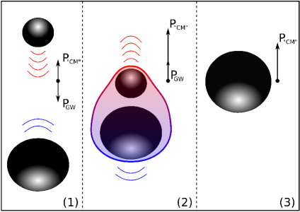
Figure 1: Generation of the antikick in the head-on collision of two unequal-mass Schwarzschild BHs as described in Rezzolla et al. (2010). Initially the smaller BH moves faster and linear momentum is radiated mostly downwards, thus leading to an upwards recoil of the system [stage (1)]. At the merger the curvature is higher in the upper hemisphere of the distorted BH (cf. red-blue shading) and linear momentum is radiated mostly upwards leading to the antikick [stage (2)]. The BH decelerates till a uniform curvature is restored on the AH [stage (3)]. This cartoon should be contrasted with the results of numerical simulations in Fig. 11.

This first article is organized as follows. Section II introduces an executive summary, where the main concepts presented in these two papers are summarized for those not wishing to enter into the mathematical details. Section III, on the other hand, extends the analysis carried out in Rezzolla et al. (2010) for RT spacetimes by considering more general initial data and by analyzing aspects of the evolution of the AH curvature. Section IV extends the methodology and diagnostic tools to BH spacetimes representing the head-on collision of unequal-mass BHs. In particular, we develop the mathematical tools necessary to measure the relevant quantities on the two screens and we show how they closely correlate. Finally, the conclusions are discussed in Sec. V, while the Appendix is used to provide details on our definitions of the correlation and matching of time series.

This paper also builds on the material presented in its companion paper II, where we present a more detailed discussion of the mathematical aspects of our framework. In particular, we revisit there the evolution of relevant geometric objects on the AH and introduce preferred null normals on a dynamical horizon. In our discussion of a newslike function on the dynamical horizon and its relation to the problem of quasilocal linear momentum, we also stress the importance of the inner horizon when evaluating fluxes across the horizon.

We use a spacetime signature $(-,+,+,+)$, with abstract index notation (first letters, $a$, $b$, $c$…, in Latin alphabet) and Latin midalphabet indices, $i,j,k...$, when making explicit the spacelike character of a tensor. Greek indices are used for expressions in particular coordinates systems. We also employ the standard convention for the summation over repeated indices. Finally, all the quantities are expressed in a system of units in which $c=G=M_{\odot}=1$, unless otherwise stated.

II The cross-correlation approach: an executive summary

As mentioned above, this section is meant to provide a general summary of the results and methodology of papers I and II, focusing mostly on the conceptual aspects and leaving aside the mathematical details, which can instead be found in the corresponding main texts.

We start by recalling that Ref. Rezzolla et al. (2010) suggested an approach to study the near-horizon nonlinear dynamics of the gravitational fields based on the systematic analysis of the deformations in the BH horizon geometry. In particular, it was shown how the gravitational dynamics responsible for the antikick after a binary merger can be understood in terms of the anisotropies in the intrinsic curvature of the AH of the resulting merged BH. Considering a RT spacetime, the kick velocity constructed from the Bondi momentum (a geometric quantity at null infinity) was put in a one-to-one correspondence with a quasilocal geometric quantity constructed on the horizon, namely, with the effective curvature parameter $K_{\mathrm{eff}}$. This geometric parameter $K_{\mathrm{eff}}$ encodes the part of the AH geometry whose dissipation through gravitational radiation can be related to the final value of the kick. Stated differently, very different binary systems, e.g., with very different mass ratio, give rise to the same final kick velocity as long as they share the same value of the $K_{\mathrm{eff}}$ parameter.

The following criteria were employed in Ref. Rezzolla et al. (2010) for the construction of the curvature parameter $K_{\mathrm{eff}}$: i) $K_{\mathrm{eff}}$ should not depend on how the AH is embedded in the spacetime; ii) $K_{\mathrm{eff}}$ should change sign (i.e., it should be an odd function) under reflection with respect to a plane normal to a given axis. From the first requirement, $K_{\mathrm{eff}}$ was constructed in terms of the intrinsic geometry of the AH, namely as a functional on the Ricci scalar ${}^{2}\!R$ associated with the induced metric on the AH. The ansatz for $K_{\mathrm{eff}}$ in Ref. Rezzolla et al. (2010), compatible with requirement ii) above and within axisymmetry, had the following structure

$$K_{\mathrm{eff}}=f_{\mathrm{even}}\left(M_{2\ell}\right)\times f_{\mathrm{odd}}\left(M_{2\ell+1}\right)\,,$$ (1)

where $M_{\ell}$’s are the so-called isolated-horizon mass multipoles associated with a spherical harmonic decomposition of ${}^{2}\!R$ in the axisymmetric case Ashtekar et al. (2004); Schnetter et al. (2006). The odd part $f_{\mathrm{odd}}$ accounts for the directionality of the kick, whereas the even part $f_{\mathrm{even}}$ controls its intensity.

In order to validate this suggestion, we analyzed a family of Robinson-Trautman (RT) spacetimes Robinson and Trautman (1962); D. Kramer and Herlt (1980), representing an (eternal) BH together with purely outgoing gravitational radiation. The mathematical properties of this class of exact solutions is already well understood Tod (1983); Singleton (1990); Chrusciel (1991, 1992), therefore this spacetime is a good test for numerical schemes Gómez et al. (1997); de Oliveira and Damiao Soares (2004) and it is an excellent toy model for problems dealing with radiation in BH environments Moreschi and Dain (1996); Moreschi et al. (2002); de Oliveira and Soares (2005); de Oliveira and Rodrigues (2008); de Oliveira et al. (2008); Aranha et al. (2008); Macedo and Saa (2008); Podolsky and Svitek (2009); Aranha et al. (2010a, b); de Oliveira et al. (2011a); Svítek (2011). Although the associated BH horizon is stationary, these RT spacetimes also contain a white-hole horizon ${\cal H}^{-}$Penrose (1973); Tod (1989); Chrusciel (1992); Chow and Lun (1999), or, more precisely, a past outer-trapping horizon Hayward (1994), whose dynamics offers a particularly well-suited scenario to test our geometric approach. This is shown in Fig. 2, which reports a Carter-Penrose diagram for the RT spacetime (see also Chrusciel (1992); Chow and Lun (1999)). The solutions exist for $u\geqslant u_{0}$ and the white hole emits GWs until the Schwarzschild spacetime is achieved asymptotically. In practice, numerical simulations run up to a finite $u_{\rm final}$ and show the exponential convergence to a solution which is essentially stationary.

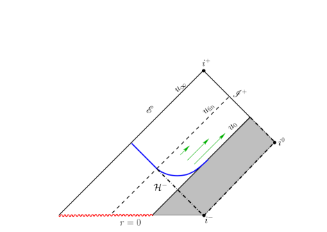
Figure 2: Carter-Penrose diagram for the RT spacetime Chrusciel (1992); Chow and Lun (1999). The solutions exist for $u\geqslant u_{0}$. The white hole emits GWs until the Schwarzschild spacetime is achieved, although the numerical simulations run until a finite $u_{\rm final}$, when an essentially stationary solution is found.

In Ref. Rezzolla et al. (2010), the functions $f_{\mathrm{even}}$ and $f_{\mathrm{odd}}$ appearing in Eq. (1) were written in the simplest possible form, i.e., as a linear expansion in $M_{\ell}$’s

$$K_{\mathrm{eff}}=\left(a_{2}M_{2}+a_{4}M_{4}+\ldots\right)\times\left(a_{3}M_{3}+a_{5}M_{5}+\ldots\right)\,.$$ (2)

Then, using suitably defined initial data, a set of numerically fitted coefficients $a_{i}$’s was found so that a one-to-one dependence between the final kick velocities $v_{\rm k}$ and $K_{\mathrm{eff}}$ at a given retarded time $u$ could be found: i.e., $\Delta v_{\rm k}=v_{\rm k}-v(u)=A\times K_{\mathrm{eff}}(u)$, where $v_{\rm k}(u)$ is the recoil velocity at time $u$ and $A$ is a constant. This injective relation between $K_{\mathrm{eff}}$ and $v_{\rm k}$ permits us to understand the degeneracy of the latter, as a function of the mass ratio in terms of AH quantities at a given (initial) time $u$ (cf. Fig. 3 in Ref. Rezzolla et al. (2010) and Fig. 9 below). Moreover, the good quantitative agreement between $v_{\rm k}$ calculated from full binary BH numerical simulations and from RT models, suggested the presence of a generic behavior in this physical process. Overall, therefore, the work in Ref. Rezzolla et al. (2010) provided an approach to understand global recoil properties in terms of (quasi-)local quantities on the AH, and an intuitive guideline to interpret the black-hole recoil properties in terms of the dissipation of AH geometric quantities.

Despite the valuable insight, the treatment presented in Ref. Rezzolla et al. (2010) had obvious limitations. First, the ansatz for $K_{\mathrm{eff}}$ in Eq. (1) is not straightforwardly generalizable to the nonaxisymmetric case. Second, the phenomenological coefficients $a_{\ell}$’s in Eq. (2) depend on the details of the employed RT initial data. Finally, the white-hole horizon analysis in RT spacetimes needs to be extended to the genuine BH horizon case. All of these restrictions are overcome in the work reported in papers I and II.

While the focus in Ref. Rezzolla et al. (2010) was on expressing the difference between the final kick velocity $v_{\infty}$ and the instantaneous kick velocity $v_{\mathrm{k}}(u)$ at an (initial) given time $u$, in terms of the geometry of the common AH at that time $u$, we here focus on geometric quantities that are evaluated at a given time during the evolution. More specifically, we will consider the variation of the Bondi linear momentum vector in time $(dP_{i}^{\mathrm{B}}/du)(u)$ as the relevant geometric quantity to monitor at null infinity ${I}^{+}$. To this scope, we need first to construct a vector $\tilde{K}^{i}_{\mathrm{eff}}(v)$ (function of an advanced time $v$) as a counterpart on the BH horizon ${\cal H}^{+}$. Then, we need to determine how $\tilde{K}^{i}_{\mathrm{eff}}(v)$ on ${\cal H}^{+}$ correlates to $(dP_{i}^{\mathrm{B}}/du)(u)$ at ${I}^{+}$.

In the RT case, the causal relation between the white-hole horizon ${\cal H}^{-}$ and null infinity ${I}^{+}$ made possible to establish an explicit functional relation between ${dv_{\mathrm{k}}}/{du}$ and $K^{\prime}_{\mathrm{eff}}(u)$. In the case of generic BH horizon, however, such a direct causal relation between the inner horizon and ${I}^{+}$ is lost (compare Fig. 2 with Figs. 3 and 4). However, since their respective causal pasts partially coincide, nontrivial correlations are still possible and expected. This can be measured through the cross-correlations of geometric quantities $h_{\mathrm{inn}}(v)$ at ${\cal H}^{+}$ and $h_{\mathrm{out}}(u)$ at ${I}^{+}$, both considered here as two time series. In particular, we will take $\tilde{K}^{i}_{\mathrm{eff}}(v)$ as $h_{\mathrm{inn}}(v)$ and $(dP_{i}^{\mathrm{B}}/du)(u)$ as $h_{\mathrm{out}}(u)$.

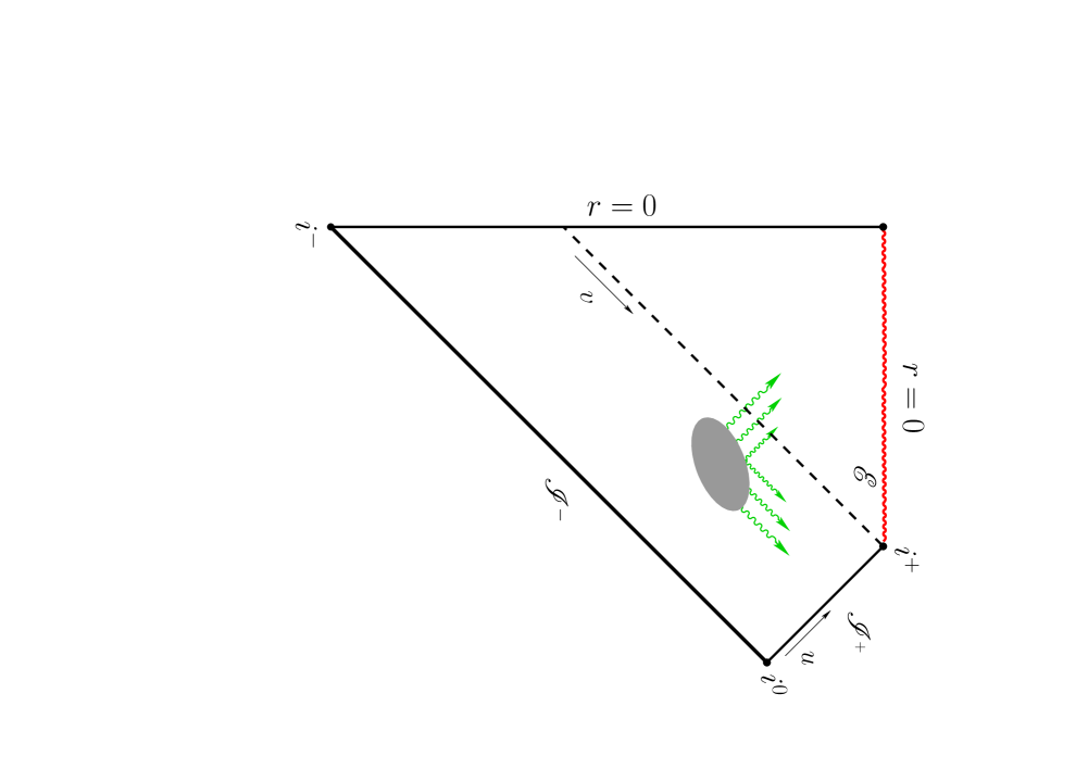
Figure 3: Carter-Penrose diagram illustrating the scattering approach to near-horizon gravitational dynamics in a generic spherically symmetric collapse. The event horizon ${E}$ and null infinity ${I}^{+}$ provide spacetime canonical screens on which geometric quantities, respectively accounting for horizon deformations and wave emission, are defined. Their cross-correlation encodes nontrivially information about the bulk spacetime dynamics.

This approach to the exploration of near-horizon gravitational dynamics resembles therefore the methodology adopted in scattering experiments. Gravitational dynamics in a given spacetime region affects the geometry of appropriately chosen outer and inner hypersurfaces of the BH spacetime. These hypersurfaces are then understood as test screens on which suitable geometric quantities must be constructed. The correlations between the two encode geometric information about the dynamics in the bulk, providing information useful for an inverse-scattering approach to the near-horizon dynamics. As a result, in asymptotically flat BH spacetimes, null infinity ${I}^{+}$ and the (event) BH horizon ${E}$ provide preferred choices for the outer and inner screens. This is nicely summarized in the Carter-Penrose diagram in Fig. 3, which illustrates the cross-correlation approach to near-horizon gravitational dynamics. The event horizon ${E}$ and null infinity ${I}^{+}$ provide natural spacetime screens on which geometric quantities, respectively, accounting for horizon deformations and wave emission, are defined. Their cross-correlation encodes information about the bulk spacetime dynamics.

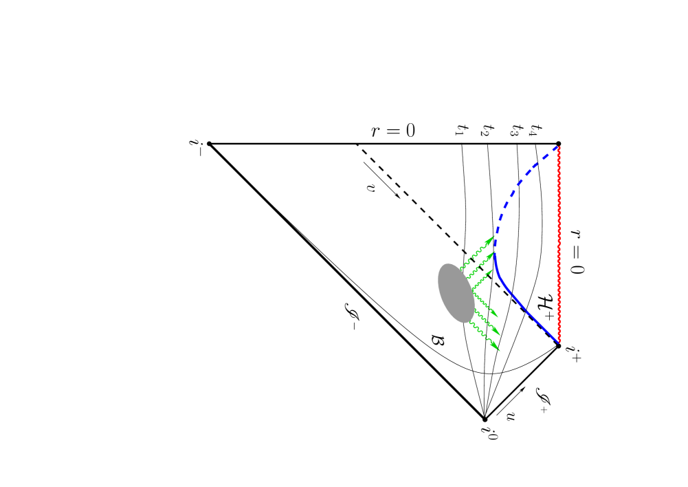
Figure 4: Carter-Penrose diagram for the scattering picture in a Cauchy initial value approach. The dynamical horizon ${\cal H}^{+}$ and a large-distance timelike hypersurface ${\cal B}$ provide inner and outer screens. Note that a the dynamical horizon is split in two portions: outer and inner (solid and dashed blue lines, respectively) and that the $3+1$ slicing sets a common time $t$ for cross-correlations.

Although the picture offered by Fig. 3 is quite simple and convincing, it is not well adapted to the 3+1 approach usually adopted in numerical studies of dynamical spacetimes. Indeed, neither the BH event horizon nor null infinity are in general available during the evolution. However, we can adopt as inner and outer screens a dynamical horizon ${\mathcal{H}}^{+}$ (future outer-trapping horizon Hayward (1994); Ashtekar and Krishnan (2003, 2004)) and a timelike tube ${\cal B}$ at large spatial distances, respectively. In this case, the time function $t$ associated with the $3+1$ spacetime slicing provides a (gauge) mapping between the retarded and advanced times $u$ and $v$, so that cross-correlations between geometric quantities at ${\mathcal{H}}^{+}$ and ${\cal B}$ can be calculated as standard time series $h_{\mathrm{inn}}(t)$ and $h_{\mathrm{out}}(t)$. This is summarized in the Carter-Penrose diagram in Fig. 4, which is the same as in Fig. 3, but where the $3+1$ slicing sets an in-built common time $t$ for cross-correlations between the dynamical horizon ${\cal H}^{+}$ (i.e., the inner screen) and a large-distance timelike hypersurface ${\cal B}$ (i.e., the outer screen).

Within this conceptual framework it is then possible to define a phenomenological curvature vector $\tilde{K}^{\mathrm{eff}}_{i}(t)$ in terms of the mass multipoles of the Ricci scalar curvature ${}^{2}\!R$ at ${\mathcal{H}}^{+}$ and show that this is closely correlated with a quantity $(dP_{i}^{\cal B}/dt)(t)$ on ${\cal B}$, representing an approximation to the variation of the Bondi linear momentum time on ${I}^{+}$. How to do this in practice for a BH spacetime is the subject of the following sections.

III Robinson-Trautman spacetimes: a toy model

We recall that the RT spacetimes are a class of solutions of the vacuum Einstein equations admitting a congruence of null geodesics which are hypersurface-orthogonal, shear-free but with nonvanishing expansion. As such, it can be regarded as a white hole emitting GWs, thus representing a valuable tool for studying the spacetime geometry in physical conditions that are similar to the final stages on the dynamics of BH binaries Robinson and Trautman (1962). The RT metric can be written as Macedo and Saa (2008)

$$ds^{2}=-\left(K-\frac{2M_{\infty}}{r}-\frac{2r\partial_{u}Q}{Q}\right)du^{2}-2dudr+\frac{r^{2}}{Q^{2}}d\Omega^{2},$$ (3)

where $Q=Q(u,\Omega)$, $u$ is a null coordinate, $r$ is an affine parameter of the outgoing null geodesics, and $d\Omega^{2}=d\theta^{2}+\sin^{2}\theta d\varphi^{2}$ is the metric of a unit sphere $S^{2}$. Here $M_{\infty}$ is a constant and is related to the mass of the asymptotic Schwarzschild BH, while the function $K(u,\Omega)$ is the Gaussian curvature of the surface with $r=1$ and $u=\mathrm{const.}$, and is given by

$$K(u,\Omega)=Q^{2}(1+\Delta^{2}_{\Omega}{\ln{Q}})\,,$$ (4)

$\Delta^{2}_{\Omega}$ being the Laplacian operator on the unit sphere $S^{2}$. The Einstein equations then lead to the RT evolution equation

$$\partial_{u}Q(u,\Omega)=-{Q^{3}}\frac{\Delta^{2}_{\Omega}K(u,\Omega)}{12M_{\infty}}\,.$$ (5)

Any regular initial data $Q=Q(u_{0},\Omega)$ will smoothly evolve according to (5) until it reaches a stationary configuration corresponding to a Schwarzschild BH at rest or moving with a constant speed Chrusciel (1991). Equation (5) implies the existence of the constant of motion $\mathcal{A}\equiv\oint_{\cal S}{d\Omega}/{Q^{2}}$, which clearly represents the area of the surface $u=\mathrm{const.}$, $r=1$ and can be used to normalize $Q$ so that $\mathcal{A}=4\pi$.

The dynamical compact object modeled by RT spacetimes is described by the past AH, which has a vanishing expansion of the ingoing future-directed null geodesics. Such past AH is described by the surface $r=R(u,\Omega)$ satisfying Penrose (1973); Tod (1989); Chow and Lun (1999)

$$Q^{2}\Delta_{\Omega}^{2}\ln{R}=K-\frac{2M_{\infty}}{R}\,.$$ (6)

The line element restricted to the AH surface $u=\mathrm{const.}$ and $r=R(\Omega)$ is

$$ds^{2}|_{{}_{\rm H}}=\frac{R^{2}}{Q^{2}}d\Omega^{2}\,,$$ (7)

which, from Eq. (6), has a Gaussian curvature

$$K_{{}_{\rm H}}=\frac{2M_{\infty}}{R^{3}}\,.$$ (8)

On the other hand, the mass and momentum are computed at future null infinity using the Bondi 4-momentum as Tod (1983); Singleton (1990); Macedo and Saa (2008)

$$P^{\alpha}(u)\equiv\frac{M_{\infty}}{4\pi}\oint_{{\cal S}_{u}}\frac{\eta^{\alpha}}{Q^{3}}d\Omega\,,$$ (9)

with $\left\{\eta^{\alpha}\right\}=\left\{1,\sin{\theta}\cos{\varphi},\sin{\theta}\sin{\varphi},\cos{\theta}\right\}$.

From now on, we restrict our problem to axisymmetry and introduce $x=\cos\theta$. Clearly, all the physically relevant information is contained in the function $Q(u,x)$, and this includes also the gravitational radiation, which can be extracted through the radiative part of the Riemann tensor Robinson and Trautman (1962); D. Kramer and Herlt (1980), which in axisymmetry is given by

$$r\Psi_{4}=\frac{Q^{2}}{2}\partial_{u}\left[\frac{(1-x^{2})\partial_{x}^{2}Q}{Q}\right]\,.$$ (10)

The dynamics of this solution can be summarized in Fig. 2, which shows the Carter-Penrose diagram for the RT spacetime. The final configuration is a stationary nonradiative solution which has the form Macedo and Saa (2008)

$$S_{\pm}(\theta)\equiv Q(\infty,\theta)=\frac{\left(1\mp v_{\rm k}x\right)}{\sqrt{1-v_{\rm k}^{2}}}\,.$$ (11)

Note that since the Bondi 4-momentum of the stationary solution is

$$P^{\alpha}(\infty)=\frac{M_{\infty}}{\sqrt{1-v_{\rm k}^{2}}}\left\{1,0,0,\pm v_{\rm k}\right\},$$ (12)

the parameter $v_{\rm k}$ in Eq. (11) is interpreted as the velocity of the Schwarzschild BH in the $z$-direction.

III.1 Mass multipoles

Given a closed 2-surface ${\cal S}$, the invariant content of its intrinsic geometry is encoded in the Ricci scalar curvature ${}^{2}\!R$ associated with the induced metric $q_{ab}$ on ${\cal S}$. Moreover, if ${\cal S}$ is an axisymmetric surface, with $\phi^{a}$ as the axial Killing vector, a preferred coordinate system $(\tilde{\theta},\tilde{\varphi})$ can be constructed such that $q_{ab}$ has the form Ashtekar et al. (2004); Schnetter et al. (2006)

$$q_{ab}dx^{a}dx^{b}=R_{{}_{\mathrm{H}}}^{2}\left(f^{-1}\mathrm{\sin}^{2}\tilde{\theta}\;d\tilde{\theta}^{2}+f\;d\tilde{\varphi}^{2}\right)\,,$$ (13)

where $f(\tilde{\theta})=q_{ab}\phi^{a}\phi^{b}/R_{{}_{\mathrm{H}}}^{2}$, with $R_{{}_{\mathrm{H}}}$ the areal radius ($A=\int_{\cal S}dA=4\pi R_{{}_{\rm H}}^{2}$). The coordinate $\tilde{\theta}$ is determined by

$$D_{a}\tilde{\zeta}=\frac{1}{R_{{}_{\mathrm{H}}}^{2}}{}^{2}\!\epsilon_{ba}\phi^{b},$$ (14)

where the coordinate $\tilde{\zeta}$ is defined by $\tilde{\zeta}\equiv\mathrm{\cos}\tilde{\theta}$ and ${}^{2}\!\epsilon_{ba}$ is the alternating symbol. In addition, the normalization condition $\oint_{\mathcal{H}}\tilde{\zeta}dA=0$ must be imposed. We note that the Ricci scalar ${}^{2}\!R$ on ${\cal S}$ can be written as Ashtekar et al. (2004)

$${}^{2}\!R=-\frac{1}{R_{{}_{\mathrm{H}}}^{2}}\frac{d^{2}f}{d\tilde{\zeta}^{2}}(\tilde{\zeta})\,,$$ (15)

and that regularity conditions on the metric impose

$$\lim\limits_{\tilde{\zeta}\to\pm 1}f(\tilde{\zeta})=0\,,\ \ \lim\limits_{\tilde{\zeta}\to\pm 1}\frac{df}{d\tilde{\zeta}}(\tilde{\zeta})=\pm 2\,.$$ (16)

A crucial feature of this coordinate system is that the associated expression for the area element is proportional to that of the “round sphere” metric $dA=R_{{}_{\mathrm{H}}}^{2}\mathrm{\sin}\tilde{\theta}\;d\tilde{\theta}d\tilde{\varphi}$. This provides the appropriate measure on ${\cal S}$ to define the standard spherical harmonics $Y_{\ell,m=0}(\tilde{\theta})$ with the standard orthonormal relations

$$\oint_{\mathcal{S}}Y_{\ell,0}(\tilde{\theta})Y_{\ell^{\prime},0}(\tilde{\theta})dA=R_{{}_{\mathrm{H}}}^{2}\delta_{\ell\ell^{\prime}}\,,$$ (17)

so that dimensionless geometric multipoles $I_{\ell}$ can be introduced as the spherical harmonics components of the Ricci scalar curvature ${}^{2}{\!}R$ Ashtekar et al. (2004)

$$I_{\ell}\equiv\frac{1}{4}\oint_{\mathcal{S}}{}^{2}\!R\;Y_{\ell,0}(\tilde{\theta})\;dA\,,\ {}^{2}\!R=\frac{4}{R_{{}_{\mathrm{H}}}^{2}}\sum_{n=0}^{\infty}I_{\ell}Y_{\ell,0}(\tilde{\theta})\,.$$ (18)

The mass multipoles $M_{\ell}$’s are then defined as appropriate dimensionful rescalings of the geometric $I_{\ell}$’s

$$M_{\ell}\equiv\sqrt{\frac{4\pi}{2n+1}}\frac{M_{{}_{\rm H}}(R_{{}_{\mathrm{H}}})^{\ell}}{2\pi}I_{\ell}\,,$$ (19)

where $M_{{}_{\rm H}}$ denotes some appropriate quasilocal mass for the surface ${\cal S}$. Because we will consider here initial data with zero angular momentum, $M_{{}_{\rm H}}$ will denote the irreducible mass $M_{\mathrm{irr}}=\sqrt{A/(16\pi)}=R_{\mathrm{H}}/2$. For later convenience, we introduce the rescaled geometric multipoles $\tilde{I}_{\ell}$

$$\tilde{I}_{\ell}\equiv\frac{1}{M_{\mathrm{irr}}^{2}}I_{\ell}=\frac{4}{(R_{{}_{\rm H}})^{2}}I_{\ell},$$ (20)

with dimensions $[\tilde{I}_{\ell}]=[\mathrm{length}]^{-2}$. The Ricci scalar curvature can then be written as

$${}^{2}\!R=\sum_{\ell=0}^{\infty}\tilde{I}_{\ell}Y_{\ell 0}\ \,.$$ (21)

A crucial remark for the discussion in Sec. IV.2 is the vanishing of the $\ell=1$ mode, i.e., $\tilde{I}_{1}=0$, which can be interpreted as a choice of center of mass frame of the AH in Ashtekar et al. (2004). This follows by first inserting expression (15) into the definition of $\tilde{I}_{1}$, so that $\tilde{I}_{1}\propto\int_{-1}^{1}f^{\prime\prime}(\tilde{\zeta})\tilde{\zeta}d\tilde{\zeta}$, and then by making use of regularity conditions (16) after integrating by parts.

In the particular case of a RT spacetime, the preferred axisymmetry coordinate system $(\tilde{\theta},\tilde{\varphi})$ is related to the RT spherical coordinates as $\tilde{\varphi}=\varphi$ and $\tilde{\theta}=\tilde{\theta}(\theta)$ satisfying

$$\partial_{\theta}\tilde{\zeta}=-\frac{\sin\theta R(\theta)^{2}}{(R_{{}_{\rm H}})^{2}Q(\theta)^{2}}\,.$$ (22)

This equation is solved with the condition $\tilde{\zeta}(0)=1$ and then one computes the mass multipoles moments through the expression

$$M_{\ell}=M_{{}_{\rm H}}\frac{(R_{{}_{\mathrm{H}}})^{\ell+1}}{2}\oint_{\cal S}\frac{P_{\ell}(\tilde{\zeta})}{Q^{2}(\theta)R(\theta)}d\Omega\,.$$ (23)

III.2 The numerical setup

As discussed in detail in Ref. Macedo and Saa (2008), for the numerical solution of the Einstein equations we introduce a Galerkin decomposition for $Q(u,x)$

$$Q(u,x)=\sum_{\ell=0}^{N}b_{\ell}(u)P_{\ell}(x),$$ (24)

where $P_{\ell}(x)$ stands for the Legendre polynomial of order $\ell$. By using standard projection techniques, Eq. (5) can be written as a system of ordinary differential equations

$$\dot{b}_{\ell}=-\frac{2\ell+1}{24M_{\infty}}\langle Q^{3}\partial_{x}\left[(1-x^{2})\partial_{x}K\right],P_{\ell}\rangle,\quad\ell=0,1,\dots,N,$$ (25)

where the inner product is given by $\langle f,g\rangle=\int_{-1}^{1}fg\,dx.$ In this way, the Cauchy problem for the RT Eq. (25) consists basically in choosing the initial value of the mode functions $b_{\ell}(u)$ according to

$$b_{\ell}(0)=\frac{2\ell+1}{2}\langle Q(0,x),P_{\ell}\rangle,$$ (26)

and then to solve the initial value problem given by (25). Note that, as $u\rightarrow\infty$, $b_{\ell}\rightarrow 0$ for $\ell>1$ and that the nonzero modes must satisfy $b_{1}(\infty)^{2}-b_{0}(\infty)^{2}=1$, with the final $v_{\rm k}$ parameter of Eq. (11) being given simply by $v_{\rm k}=-b_{1}(\infty)/b_{0}(\infty)$.

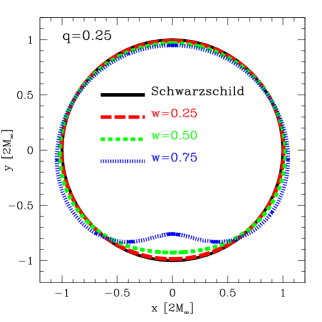
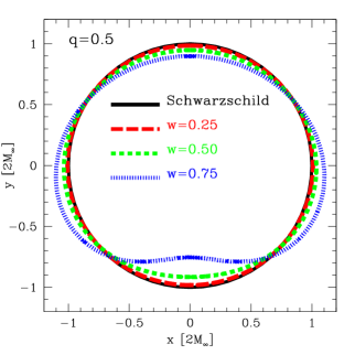
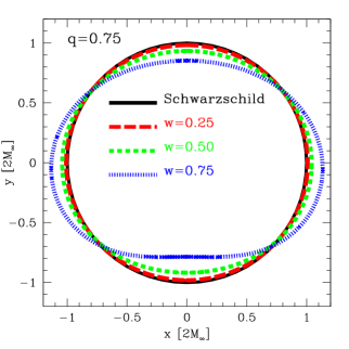
Figure 5: AH of the head-on initial data given in Eq. (28). The parameters $q$ and $w$ control the deformation of the surfaces. The final configuration is a Schwarzschild BH (continuous black line) and it is achieved after the deformation is dissipated with the emission of GWs. Our results confirm the interpretation given Aranha et al. (2008) for $q$ as the mass ratio of the BHs. However, we attach no physical meaning to $w$ as done in Aranha et al. (2008), for RT models a single deformed horizon, and nothing can be said about the velocities of the individual colliding BHs.

Equation (6) can be solved for the horizon $R(u,\theta)$ either by imposing regular conditions on the boundary $\partial_{\theta}R(0)=0$ and $\partial_{\theta}R(\pi)=0$ and using an ordinary shooting method to find $R(0)$ and $R(\pi$), or by following the approach in de Oliveira et al. (2011b) introducing another Galerkin decomposition on the horizon and truncated at the order $N_{\text{H}}$

$$\ln{\frac{R}{2M_{\infty}}}=\sum_{\ell=0}^{N_{\text{H}}}c_{\ell}(u)P_{\ell}(x).$$ (27)

The projection of Eq. (6) on the basis of the Legendre polynomials couples the known Galerkin modes $b_{\ell}$ with the unknown coefficients $c_{\ell}$ and the resulting algebraic nonlinear system can be easily solved via a Newton-Raphson method.

III.3 The initial data

In general, any family of regular functions $Q$, i.e., $0<Q(u_{0},x)<\infty,~{}\forall x\in[-1,1]$ can be used as an initial data for the RT spacetime. For any of such family, one can set a parameter $Q_{0}$ to ensure the constant of motion to be $\mathcal{A}=4\pi$. Moreover, the deformed BH will not be initially at rest in general. As a result, given the initial velocity $v_{\rm k,0}\equiv P^{3}(0)/P^{0}(0)$, we perform a boost ${\overline{P}}^{\alpha}={\Lambda^{\alpha}}_{\beta}(v_{\rm k,0})P^{\beta}$ with ${\Lambda^{\alpha}}_{\beta}(v_{\rm k,0})$ the associated Lorentz transformation, so that ${\overline{P}}^{3}(0)=0$ by construction. The kick velocity is then defined at any time as $v(u)=\overline{P}^{3}(u)/\overline{P}^{0}(u)$.

Despite this overall simplicity, the definition of initial data that is physically meaningful represents one of the main difficulties in the study of RT spacetimes. Since we are here more interested in a proof of principle than in describing a realistic configuration, we have adopted both a prescription reminiscent of a “head-on” collision of two BHs Aranha et al. (2008) and a new variant of it.

III.3.1 “Head-on” initial data

As a first set of initial data we consider the one developed in Ref. Aranha et al. (2008)

$$Q(0,\theta)=Q_{0}\left[\frac{1}{\sqrt{1-wx}}+\frac{q}{\sqrt{1+wx}}\right]^{-2},$$ (28)

which was interpreted to represent the final stages (i.e., after a common AH is formed) of a head-on collision of two boosted BHs with opposite velocities $w\in[-1,1]$ and mass ratio $q\in[0,1]$ Aranha et al. (2008). Figure 5 shows the shape of the surface $R(u_{0},\tilde{\theta})$ for different values of those parameters. It is worth remarking that despite the name, this initial data does not represent a binary system but is, strictly speaking, only a distorted horizon. In a more conservative approach, one can regard $q$ and $w$ just as free parameters that control the deformation on the horizon, and this is the view we will adopt hereafter. However, a number of interesting analogies with the head-on collision of two BHs have been suggested Aranha et al. (2008, 2010b), and will be further discussed below.

The interpretation of $q$ as a mass-ratio parameter is not totally unreasonable. For instance, Fig. 3 of Rezzolla et al. (2010) showed the final value of the velocity in RT spacetime evolved from the head-on initial data against the reduced mass ratio $\nu\equiv q/(1+q)^{2}$. The curve obeys the distribution

$$v_{\rm k}=A\nu^{2}\sqrt{1-4\nu}(1+B\nu),$$ (29)

as found in all numerical simulations Rezzolla (2009), with the value of $A$ and $B$ depending on the particular choice of $w$.

Since the solution does not exist for $u<u_{0}$, it is impossible to assign a value for $w$ that could account for any previous stages on the evolution of the binary. With the original interpretation of $w$ as the velocities of the BHs, a first trivial estimate, as proposed by Moreschi and Dain (1996), is to assume a Newtonian evolution of two particles with masses $M_{1}$ and $M_{2}$, which start at rest at an initial distance $L_{0}$. At a given distance $L$, in the frame where $v_{1}=-v_{2}=w$ one has

$$w=\sqrt{\frac{1}{2}\left(\frac{M}{L}-\frac{M}{L_{0}}\right)},$$ (30)

with $M=M_{1}+M_{2}$. Choosing $L_{0}\simeq 6\,M$ and $L\simeq 2\,M$, one obtains $w\simeq 0.41$. Furthermore, still in Ref. Rezzolla et al. (2010) it was shown that $w=0.425$ presents a surprisingly good match with some results found in the close-limit approximation, where the initial data for the ringdown phase was given by a previous plunge with the BHs inspiralling towards each other from the innermost circular orbit until $\thicksim 2M$ Le Tiec et al. (2010).

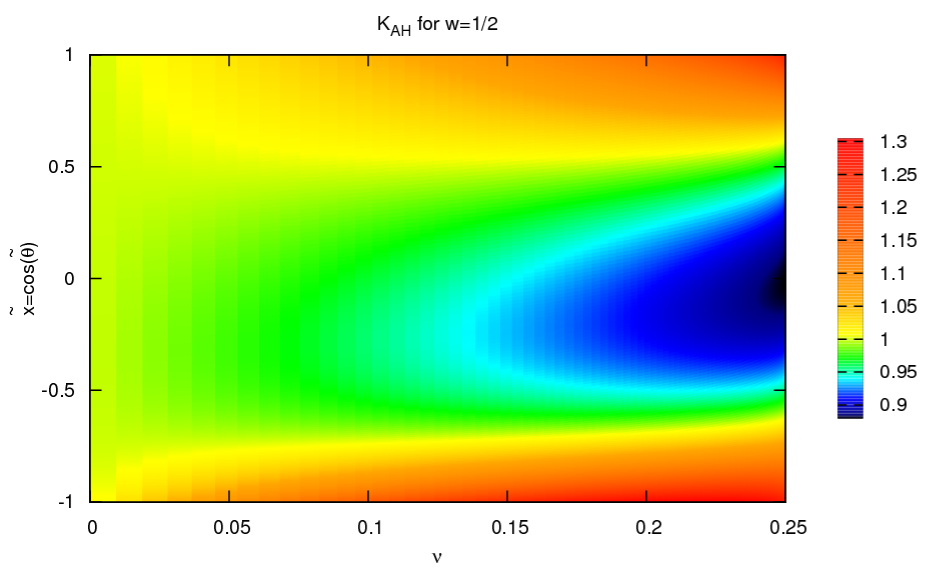
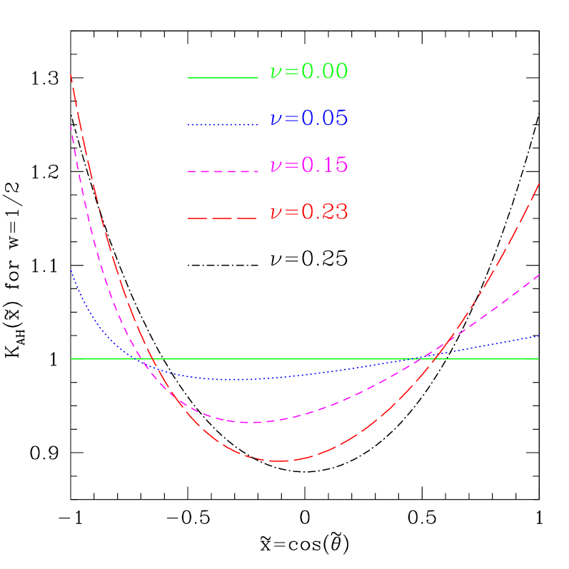
Figure 6: Left panel: Horizon mean curvature $K_{{}_{\rm H}}$ for $w=1/2$ shown as a function of reduced mass ratio $\nu$ and of the polar angle $x=\cos\theta$. Note that the distribution is symmetric with respect to the equatorial plane for $\nu=0$ and $\nu=1/4$. Right panel: Horizon curvature for some representative values of the reduced mass ratio. The low-$\nu$ branch is characterized by large curvature gradients across the AH but small values of the curvature, while the high-$\nu$ branch small curvature gradients and large values of the curvature Rezzolla et al. (2010).

It is important to remark that one should not expect a complete agreement between the values of $A$ and $B$ from the head-on collision in RT spacetimes with the ones found in numerical-relativity calculations of binary BHs in quasicircular orbits Gonzalez et al. (2007a). The first ones, in fact, (and modulo the interpretative issues discussed above) can only account for the post-merger phase, while the second ones account for the whole recoil. A complete discussion on the dependence of $A$ and $B$ with respect to $w$ can be found in Aranha et al. (2010b). For the sake of convenience we will fix $w=0.5$, but our results do not depend upon this choice. The substitution $w\rightarrow-w$ just changes the sign of the recoil velocity.

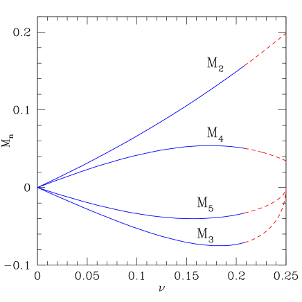
Figure 7: Lower-order mass moments for $w=1/2$. Note that they all vanish at $\nu=0$, while only the odd ones are zero for $\nu=1/4$. As in Fig. 3 of Rezzolla et al. (2010), the colors represent the two different branches composing the curve $v_{\rm k}$ versus $\nu$. The color changes at the mass ratio for which the recoil velocity is at a maximum.

The relation between the kick velocity and the reduced mass ratio expressed by Eq. (29) has a peak $v_{\rm k}^{\rm max}$ for $\nu^{\rm max}\approx 0.195$ Gonzalez et al. (2007a). As the recoil vanishes for $\nu=0$ and $\nu=1/4$, there will always be two values of the mass parameter leading to the same recoil when $v<v_{\rm k}^{\rm max}$. It is natural to wonder whether two completely different systems (namely systems with different mass ratios) share some common physical property which could lead to the same recoil. Thinking in terms of the horizon’s intrinsic deformation provides a simple way to explain this degeneracy. System with $\nu<\nu^{\rm max}$, in fact, are characterized by large curvature gradients across the AH but small values of the curvature, while system with $\nu>\nu^{\rm max}$ are characterized by small curvature gradients and large values of the curvature. This intuitive picture can be best appreciated in Fig. 6, which reports the horizon mean curvature $K_{{}_{\rm H}}$ for $w=1/2$ as a function of reduced mass ratio $\nu$ and of the polar angle $\tilde{x}=\cos\tilde{\theta}$ (left panel) or for some representative values of the reduced mass ratio (right panel). Note that the low-$\nu$ branch is characterized by large curvature gradients between the north and south poles of the AH, but small values of the curvature, while the high-$\nu$ branch is characterized by small curvature gradients and large values of the curvature. As discussed in Ref. Rezzolla et al. (2010), it is the product of the deformations on the horizon with the gradients across the equator that yields the same recoil for two apparently different systems.

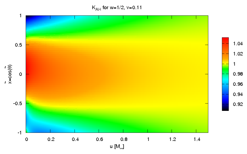
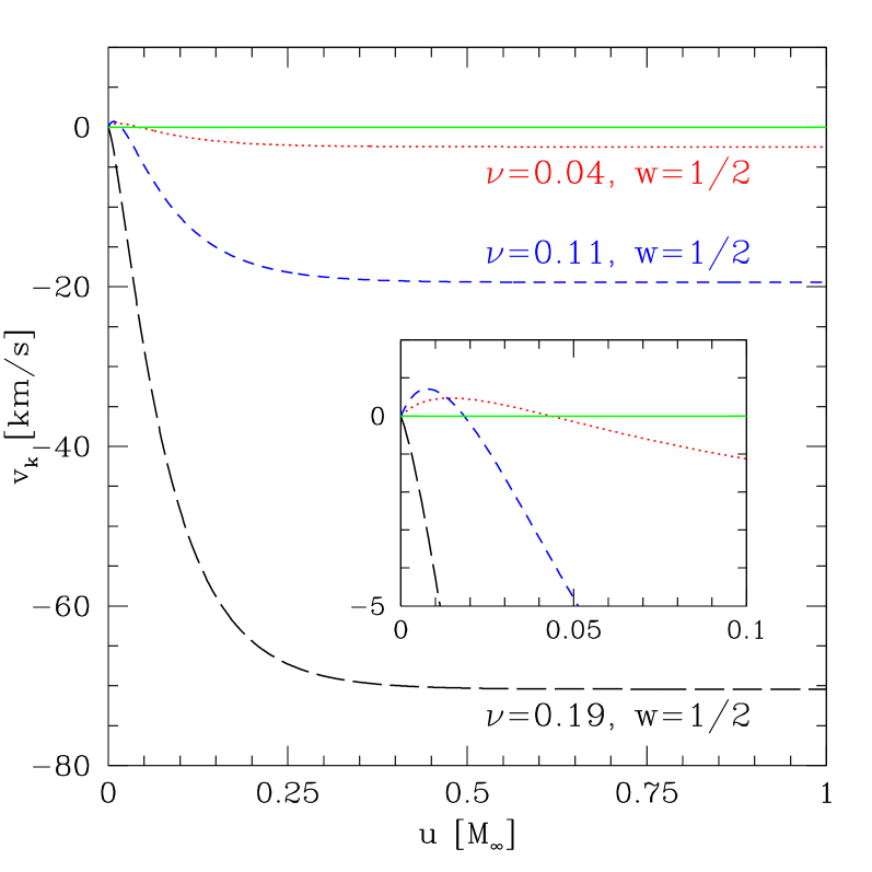
Figure 8: Left panel: Curvature evolution for the distorted-AH initial data with $w=1/2,\nu=0.11$. Note the small curvature excess at the south pole, which is rapidly radiated away to yield an almost uniform distribution after $u/M_{\infty}\simeq 1.5$. Right Panel: evolution of the recoil velocity for representative values of the parameter $q$, some of which lead to no-monotonic changes in the velocity.

Complementary information to the one in the left panel of Fig. 6 is depicted in Fig. 7, which shows the typical behavior of the lower-order mass moments as a function of the reduced mass ratio. Notice they all vanish for $\nu=0$, since this configuration represents an undistorted BH. For $\nu=1/4$, on the other hand, only the odd modes are zero, indicating that the configuration is symmetric with respect to the equatorial plane and the emission of GW will not give rise to a recoil. Also note that the maximum of the odd modes does not correspond to the mass ratio at which the recoil velocity reaches its highest value. Even though a net emission of momentum will only take place when there is an asymmetry on the horizon across the equator (i.e., $M_{\rm odd}\neq 0$), the intensity of the emission will also depend on how deformed the BH is (i.e., $M_{\rm even}\neq 0$).

Without loss of generality, we can use the even modes to measure overall distortions on the horizon, while the odd ones measure the asymmetries between the north and south hemispheres. To account for both contributions, we constructed in Rezzolla et al. (2010) an effective-curvature parameter as the product of two functions depending solely on the even or the odd modes, i.e., $K_{\mathrm{eff}}=f_{\mathrm{even}}\left(M_{2n}\right)\times f_{\mathrm{odd}}\left(M_{2n+1}\right)$. This quantity represents a measure of the global curvature properties of the initial data, from which the recoil depends in an injective way. Indeed, Fig. 4 in Rezzolla et al. (2010) showed that with a suitable choice of coefficients, i.e., $K_{\rm eff}=M_{2}|\sum_{n=1}M_{2n+1}/3^{n-1}|$, the correlation between $K_{\rm eff}$ measured at the initial time against the final velocity is actually linear.

III.3.2 Distorted-AH initial data

The evolution produced by the head-on initial data (28) leads to a monotonic increase/decrease of the recoil velocity once the initial data is specified on the white hole. However, a more complex (i.e., nonmonotonic) dynamics can be easily produced through a simple variation of the head-on initial data. We refer to this new family of initial conditions as to the “distorted AHs” and we express them as

$$Q(u_{0},x)=Q_{\text{HO}}(x;q,w)+qx^{2}Q_{\text{HO}}(x;q,-w),$$ (31)

where $Q_{\text{HO}}(x;q,w)$ corresponds to the head-on initial data (28). Clearly, this is just a mathematical choice and no physical significance can be associated to this initial data.

Note that (31) maintains the symmetries provided by the mass-ratio parameter $q$: for $q=0$ one recovers the nondeformed Schwarzschild BH and $q=1$ gives an even initial data, i.e., $Q(u_{0},x)=Q(u_{0},-x)$, which leads to a zero final recoil. Furthermore, note that the resulting recoil velocity does not lead to the scaling expressed by Eq. (29), thus giving strength to the idea that the head-on initial data is closely related to the merger of a binary system as proposed in Refs. Aranha et al. (2008, 2010b).

As anticipated, the use of this initial data leads to a more interesting dynamics and this is shown in Fig. 8, whose left panel reports the curvature evolution for $w=1/2$ and $\nu=0.11$, while the right panel reports the evolution of the recoil velocity for representative values of the parameter $q$, some of which lead to nonmonotonic changes in the velocity. Note the small curvature excess at the south pole, which is rapidly dissipated as GWs are emitted so as to yield an almost uniform distribution. As pointed out in Rezzolla et al. (2010), the velocity reaches its final value when there is no asymmetry in the deformation between the north ($\tilde{x}>0$) and south ($\tilde{x}<0$) hemispheres, i.e., after $u/M_{\infty}\simeq 0.5$.

To prove that the approach discussed in the previous subsection is indeed generic, we define an effective curvature $K_{\mathrm{eff}}$ also for this family of initial data, again in terms of the product of odd and even mass moments

$$K_{\rm eff} = (M_{2}+a_{4}\,M_{4}+a_{6}\,M_{6}+a_{8}\,M_{8}+a_{10}\,M_{10})\times(M_{3}+a_{5}\,M_{5}+a_{7}\,M_{7}+a_{9}\,M_{9})\,,$$ (32)

to find that the set of coefficients $a_{4}=0.304,a_{6}=0.178$, $a_{8}=0.086,a_{10}=-0.186$ and $a_{5}=0.076,a_{7}=-0.090$, $a_{9}=-0.183$ leads to the expected injective, and actually linear, behavior. Clearly, and as it is also natural to expect, the coefficients are different from those found for the head-on initial data, and they will always depend upon the specific family of initial data considered. The remarkable feature though, is that they remain constant in time. This is illustrated in Fig. 9, which shows that the effective curvature (32) is still linear with respect to the relative velocity $\Delta v_{\rm k}(u)\equiv v(u_{\infty})-v(u)$ at any time during the evolution (this is shown by the different coloured symbols, each of which refers to a specific time) and also at late times (see inset). This time-independent property is general, and not limited to this particular family of initial data. In particular, it is also found, for instance, in the head-on case. This result reflects the fact that the deformations of the horizon evolve in time in a self-similar manner, so that although the ranges for $K_{\rm eff}$ change in time (becoming smaller as the deformations are radiated away), the corresponding recoil velocities maintain the same proportionality (cf. Fig. 9).

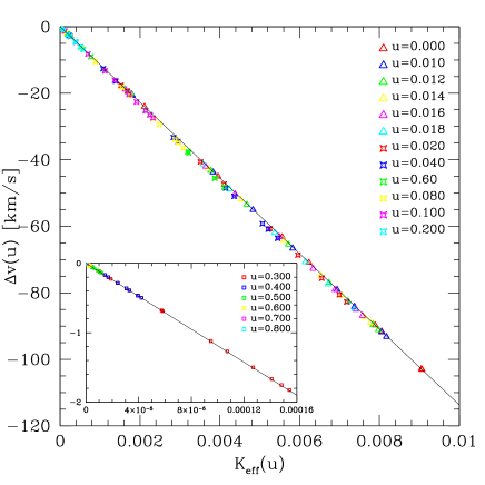
Figure 9: Difference $\Delta v_{\rm k}(u)\equiv v_{\rm k}(u_{\infty})-v_{\rm k}(u)$ against the effective-curvature parameter for several values of the “initial” time $u$. The linear relation between the effective curvature (32) and the kick velocity is preserved along the evolution as indicated by the different symbols, each representing a specific time in the evolution. This remains the case also at late times as shown in the inset.

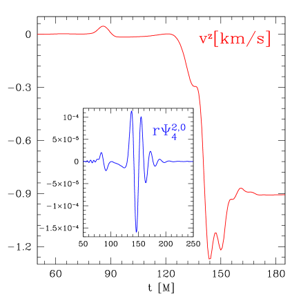
Figure 10: Evolution of the velocity (red curve) measured with the flux of momentum carried out by the GWs. Note the antikick at about $t/M\approx 145$ that decelerates the system before the final kick velocity is reached. The GW signal is instead shown in the inset, namely the dominant $\Psi_{4}^{2,0}$ multipole (blue curve).

As a concluding remark, we can summarize as follows the insight gained through the study of RT spacetimes: the construction of the effective-curvature parameter depends quantitatively on the family of initial data considered, but that for any choice of data, it is possible to find an explicit expression that relates the effective-curvature parameter to the (final) recoil velocity through a one-to-one mapping. What however will not depend on the initial data is the functional dependence of the effective-curvature parameter as expressed by (1). Indeed, in the next section we will generalize the idea and functional form of the effective-curvature parameter to account for the dynamics in binary BH spacetimes.

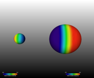
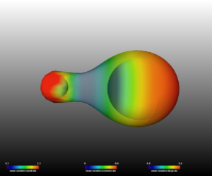
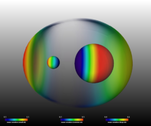
Figure 11: Realization of the cartoon in Fig. 1 with numerical data from a simulation of head-on collision with mass ratio $q=1/2$. The color code shows the mean curvature on the apparent horizons, which has the same anisotropic behavior of the intrinsic curvature. As described in Fig.1, once the common horizon is formed, the curvature is stronger in the region of the smaller BH and is dissipated during the evolution.

IV Black-Hole spacetimes: Head-on collisions

IV.1 Numerical Setup and Results

The numerical solution of the Einstein equations has been performed using a three-dimensional finite-differencing code solving a conformal-traceless “$3+1$” BSSNOK formulation of the Einstein equations (see Pollney:2009yz1 for the full expressions) using the Einstein Toolkit (ein, ), the Carpet (Schnetter et al., 2004) adaptive mesh-refinement driver, AHFinderDirect Thornburg (2004) to track the AHs, and QuasiLocalMeasures Dreyer et al. (2003) to evaluate the mass multipoles associated with them. Recent developments, such as the use of $8$th-order finite-difference operators or the adoption of a multiblock structure to extend the size of the wave zone have been recently presented in Pollney et al. (2009); Pollney:2009yz1. Here, however, to limit the computational costs and because a very high accuracy in the waveforms is not needed, the multiblock structure was not used. Also, for compactness we will not report here the details of the formulation of the Einstein equations solved for the form of the gauge conditions adopted. All of these aspects are discussed in detail in Pollney:2009yz1, to which we refer the interested reader.

Our initial data consists of head-on (i.e., zero angular momentum) Brill-Lindquist initial data with a mass-ratio of $q=1/2$. The initial separation of both BHs is $10M$ and they are initially located at $(0,0,6.6666$) and $(0,0,-3.3333)$ to reflect their center-of-mass offset. Both BHs have no angular nor linear momentum initially. We use a 3D Cartesian numerical grid with seven levels of mesh-refinement for the higher mass and eight levels of mesh-refinement for the lower mass BH. The resolution of our finest grid is $h=M/64$, while the angular grid used to find the AHs and evaluate any property on these 2-surfaces has a resolution of $65$ points in $\varphi$-direction and $128$ points in $\theta$-direction. The extraction of GWs is performed calculating $\Psi_{4}$ at finite-radius detection spheres with radii of $r_{1}=60\,M\,,r_{2}=85\,M$ and $r_{3}=145\,M$ and then extrapolating to infinity.

Some of the most salient results of the numerical simulations are summarized in Fig. 10, which reports the evolution of the recoil velocity (red curve) measured with the flux of momentum carried out by the GWs. Note the development of the antikick at about $t/M\approx 145$ (followed by several smaller oscillations) that decelerates the BH before the final kick velocity is reached. Also shown in the inset is GW signal in its larger multipolar component $\Psi_{4}^{2,0}$ (blue curve). Similarly, Fig. 11 provides a realization of the cartoon in Fig. 1 with numerical data from a simulation of head-on collision with mass ratio $q=1/2$. Shown with a color code is the mean curvature on the apparent horizons, which shares the same qualitative properties, and in particular the anisotropic behavior, of the intrinsic curvature. As intuitively described in Fig.1, once the common horizon is formed, the curvature is stronger in the region of the smaller BH and is dissipated as the evolution proceeds. Note that the curvature distribution is anisotropic already at the beginning, as the BHs are tidally distorting each other.

IV.2 Geometric quantities at the BH horizon: $\tilde{K}^{\mathrm{eff}}_{i}(t)$

As discussed in Secs. I and II, the analysis of the recoil dynamics in generic BH spacetimes requires a shift with respect to the methodology used in RT spacetimes. When considering standard $3+1$ numerical solutions of BH spacetimes, in fact, we study the near-horizon dynamics responsible for the BH recoil in terms of the time cross-correlations between a vector $(dP_{i}^{\cal B}/dt)(t)$ at a large-radius hypersurface ${\cal B}$ and an effective-curvature vector $\tilde{K}^{\mathrm{eff}}_{i}(t)$ constructed from the intrinsic geometry on the dynamical BH horizon ${\cal H}^{+}$. The vector $(dP_{i}^{\cal B}/dt)(t)$ on ${\cal B}$ approximates the Bondi linear momentum flux $(dP_{i}^{\mathrm{B}}/dt)(t)$ at ${I}^{+}$. From now on we will systematically refer to $(dP_{i}^{\mathrm{B}}/dt)(t)$ (and to ${I}^{+}$ instead of ${\cal B}$), understanding that we are actually using an approximation.

The construction of $\tilde{K}^{\mathrm{eff}}_{i}(t)$ at ${\cal H}^{+}$ is based on the following two guidelines: a) $\tilde{K}^{\mathrm{eff}}_{i}(t)$ is built out of the intrinsic geometry Ricci scalar curvature ${}^{2}\!R$ on ${\cal H}^{+}$ sections; b) the functional form of $(dP_{i}^{\mathrm{B}}/dt)(t)$ in terms of the geometry at ${I}^{+}$ guides the choice of the functional dependence of $\tilde{K}^{\mathrm{eff}}_{i}(t)$ on ${}^{2}\!R$. The first requirement is motivated by the success in the RT case, whereas the second one aims at preserving those basic structural features of the specific function to be cross-correlated.

Following these guidelines, we start by expressing the flux of Bondi linear momentum at null infinity. In terms of a retarded time $u$ parameterizing ${I}^{+}$, its Cartesian components can be written as

$$\frac{dP_{i}^{\mathrm{B}}}{du}(u)=\lim\limits_{(u,r\to\infty)}\frac{r^{2}}{8\pi}\oint_{{\cal S}_{u,r}}s_{i}\;|{\cal N}(u,\Omega)|^{2}d\Omega\,,$$ (33)

where $r$ parameterizes the large-radius spheres ${\cal S}_{u,r}$ along a $u=\mathrm{const.}$ hypersurface, $r^{2}d\Omega$ is the area element on ${\cal S}_{u,r}$, $s^{i}$ is its normal unit vector with Cartesian components $s^{i}=\left(\mathrm{\sin}\theta\mathrm{\cos}\varphi,\mathrm{\sin}\theta\mathrm{\sin}\varphi,\mathrm{\cos}\theta\right)$, and the news functions ${\cal N}(u)$ can be expressed in terms of the Weyl scalar $\Psi_{4}$ as

$${\cal N}(u,\Omega)=\int_{-\infty}^{u}\Psi_{4}(u^{\prime},\Omega)du^{\prime}\,.$$ (34)

In our $3+1$ setting with an outer boundary at a finite spatial distance we need to express the flux with respect to the time function $t$ parameterizing the spatial slices $\Sigma_{t}$, so that we replace ${\cal S}_{u,r}$ with ${\cal S}_{t,r}$

$$\frac{dP_{i}^{\mathrm{B}}}{dt}(t)=\lim\limits_{r\to\infty}\frac{r^{2}}{16\pi}\oint_{{\cal S}_{t,r}}s_{i}\left|\int_{-\infty}^{t}\Psi_{4}(t^{\prime},\Omega)dt^{\prime}\right|^{2}d\Omega\,,$$ (35)

and where we can think of $t$ (related to $u$ by $u=t-r$ near ${I}^{+}$) as parameterizing the cuts of ${I}^{+}$ by hyperboloidal slices or, alternatively, the cuts of the timelike hypersurface ${\cal B}$ approximating ${I}^{+}$ at large $r$. We can now rewrite expression (35) in terms of a generic vector $\xi^{i}$ transverse to ${\cal S}_{u,r}$ (i.e., with a generically nonvanishing component along the normal to ${\cal S}_{u,r}$), so that the component of the flux of Bondi linear momentum along $\xi^{i}$ is

$$\frac{dP^{\mathrm{B}}[\xi]}{dt}(t)=\lim\limits_{r\to\infty}\frac{r^{2}}{16\pi}\oint_{{\cal S}_{t,r}}(\xi^{i}s_{i})\left|\int_{-\infty}^{t}\Psi_{4}(t^{\prime},\Omega)dt^{\prime}\right|^{2}d\Omega\,.$$

We take this expression as the starting point for the construction of $\tilde{K}^{\mathrm{eff}}_{i}$. It provides the functional form of the Bondi linear momentum flux in terms of the relevant component of the Riemann tensor at ${I}^{+}$, namely $\Psi_{4}$. Then, the two above-mentioned guidelines for the construction of $\tilde{K}^{\mathrm{eff}}_{i}$ can be met by considering a heuristic substitution of $\Psi_{4}$ by ${}^{2}\!R$ in expression (IV.2).

It is important to note that in the same way in which the outgoing null coordinate $u$ parameterizes naturally ${I}^{+}$, the ingoing null coordinate $v$, which runs along ${I}^{-}$, is a natural label to parameterize the horizon ${\cal H}^{+}$. However, within our $3+1$ setting, we use Eq. (IV.2) as the ansatz leading to the following proposal for the component $\tilde{K}_{\mathrm{eff}}[\xi](t)$ of $\tilde{K}^{\mathrm{eff}}_{i}(t)$ along a vector $\xi^{i}$ (tangent to the slice $\Sigma_{t}$) transverse to the section ${\cal S}_{t}$ of ${\cal H}^{+}$

$$\tilde{K}^{\mathrm{eff}}[\xi](t)\equiv-\frac{1}{16\pi}\oint_{{\cal S}_{t}}(\xi^{i}s_{i})\left|\tilde{\cal N}(t,\Omega)\right|^{2}dA\,,$$ (37)

with

$$\tilde{\cal N}(t,\Omega)\equiv\int_{t_{c}}^{t}{}^{2}\!R(t^{\prime},\Omega)dt^{\prime}+\tilde{\cal N}^{t_{c}}(\Omega)\,.$$ (38)

In the equations above, $dA$ is the area element of ${\cal S}_{t}$, the global negative sign accounts for the relative change of the orientation of outgoing vector normal to inner and outer boundary spheres, $s^{i}$ are the components of the unit normal vector to ${\cal S}_{t}$ tangent to $\Sigma_{t}$, and $\tilde{\cal N}^{t_{c}}(\Omega)$ is a generic function on the surface to be fixed.

Some remarks are in order concerning expressions (37) and (38). First, there is a clear asymmetry between expressions (IV.2) and (37) when substituting the complex quantity $\Psi_{4}$ at ${I}^{+}$ (encoding two independent modes corresponding to the GW polarizations) by the real quantity ${}^{2}\!R$ on the inner horizon (a single dynamical mode). Inspection of Eq. (IV.2) immediately suggests an alternative to ${}^{2}\!R$ by the natural inner boundary analogue of $\Psi_{4}$, i.e., $\Psi_{0}$. However, this strategy must face the issue of identifying an appropriate null tetrad at ${\cal H}^{+}$ for the very construction of $\Psi_{0}$. Second, the lower limit in the time integration, $t\to-\infty$, appearing in Eq. (IV.2) must be replaced by the time $t_{c}$ of first appearance of the common horizon, when quantities as ${}^{2}\!R(t,\Omega)$ start to be well-defined. However, there is still a deeper difference between ${\cal N}(t,\Omega)$ and $\tilde{\cal N}(t,\Omega)$. Even though one can construct the former as in Eq. (34), i.e., as the time integral of $\Psi_{4}$, the definition of the news function is local in time depending only on quantities on ${\cal S}_{t}$ and not requiring the knowledge of the past history of ${I}^{+}$. The latter though is here defined as the time integral of ${}^{2}\!R$ and there is no reason to expect the same local-in-time behavior, specially as $t\rightarrow\infty$. In particular, we fix the function $\tilde{\cal N}^{t_{c}}(\Omega)$ by imposing $\displaystyle\lim_{t\rightarrow\infty}\tilde{\cal N}(t,\Omega)=0$.

All the points raised above are addressed in detail in the accompanying paper II and we adopt here a purely effective approach to $\tilde{K}_{\mathrm{eff}}^{i}(t)$, since ${}^{2}\!R$ represents an unambiguous geometric object that captures the (possibly many, if matter is included) relevant dynamical degrees of freedom in a single effective mode. Ultimately, this heuristic proposal for the effective curvature is acceptable only as long as it can be correlated with $dP_{i}^{\mathrm{B}}/dt$, and this is what we will show in the following.

IV.2.1 Axisymmetric BH spacetimes

As a first application of the ansatz (37), we consider the axisymmetric case of the head-on collision of two BHs with unequal masses. We adopt therefore a coordinate system $(r,\theta,\varphi)$ adapted to the horizon ${\cal H}^{+}$ so that $r=\mathrm{const.}$ characterizes sections ${\cal S}_{t}$ and we can write $s_{i}=MD_{i}r$, with $M^{-2}=D_{i}rD^{i}r$ (i.e., $M^{-2}=\gamma^{rr}$). Then, taking advantage of the axisymmetry, we adopt on ${\cal S}_{t}$ the preferred coordinated system $(\tilde{\theta},\tilde{\varphi)}$ discussed in Sec. III.1 and consider the Cartesian-like coordinates constructed from $(r,\tilde{\theta},\tilde{\varphi})$ by standard spherical coordinates relations: $x=r\,\mathrm{\sin}\tilde{\theta}\,\mathrm{\cos}\tilde{\varphi},y=r\,\mathrm{\sin}\tilde{\theta}\,\mathrm{\sin}\tilde{\varphi},z=r\,\mathrm{\cos}\tilde{\theta}$. In these coordinates we have $s_{i}=M(\mathrm{\sin}\tilde{\theta}\,\mathrm{\cos}\tilde{\varphi},\mathrm{\sin}\tilde{\theta}\,\mathrm{\sin}\tilde{\varphi},\mathrm{\cos}\tilde{\theta})$. Assuming the $z$-axis to be adapted to the axisymmetry, we choose $\xi^{i}$ in Eq. (37) as $(\xi_{z})^{i}=M^{-1}(\partial_{z})^{i}$, so that $(\xi_{z})^{i}s_{i}=\mathrm{\cos}\tilde{\theta}$. Inserting expression (21) in Eqs. (37) and (38) we obtain

$$\tilde{K}_{z}^{\mathrm{eff}}(t) \equiv \tilde{K}^{\mathrm{eff}}[\xi_{z}](t)=$$

$$= -\frac{1}{16\pi}\oint_{{\cal S}_{t}}(\mathrm{\cos}\tilde{\theta})\left(\sum_{\ell=0}^{\infty}\tilde{\cal N}_{\ell}(t^{\prime})Y_{\ell,0}(\tilde{\theta})dt^{\prime}\right)^{2}dA,$$

with

$$\tilde{\cal N}_{\ell}(t)\equiv\int_{t_{c}}^{t}dt^{\prime}\tilde{I}_{\ell}(t^{\prime})+\tilde{\cal N}_{\ell}^{t_{c}}\ ,$$ (40)

being the coefficients of a multipolar expansion of Eq. (38). Inserting the form $dA=R^{2}_{\mathrm{H}}\mathrm{\sin}\tilde{\theta}d\tilde{\theta}d\tilde{\varphi}$ of the area element on ${\cal S}_{t}$ and performing the angular integration we finally find

$$\tilde{K}^{\mathrm{eff}}_{z}(t)=-\frac{R_{\mathrm{H}}^{2}}{16\pi}\sum_{\ell=2}\tilde{\cal N}_{\ell}\left(D^{(0)}_{\ell,0}\tilde{\cal N}_{\ell-1}+D^{(0)}_{\ell+1,0}\tilde{\cal N}_{\ell+1}\right)\,,$$ (41)

with

$$D^{(0)}_{\ell,0} \equiv \frac{\ell}{\sqrt{(2\ell+1)(2\ell-1)}}\,.$$ (42)

As for the definition of $K_{\mathrm{eff}}$ in the RT case, Eq. (41) is quadratic in the (geometric) mass multipoles, i.e., the spherical harmonic components of the intrinsic curvature Ricci scalar curvature ${}^{2}\!R$, although it involves a time integration, absent in (2). Also, it is an odd function under reflection with respect to $z=\mathrm{const.}$ planes and it involves only products of odd and even multipoles, precisely one of the criteria for the construction of $K_{\mathrm{eff}}$ leading to the ansatz in Eq. (1). In essence, expression (41) for $\tilde{K}^{\mathrm{eff}}_{z}$ fulfills the two basic requirements for the curvature parameter $K_{\mathrm{eff}}$ with the added value that it is fully general and, in contrast with (2), no phenomenological parameters need to be fitted. An additional and crucial feature is that terms involving $\ell=0,1$ are absent, due to the vanishing of $\tilde{I}_{1}$ as discussed after Eq. (21).

The quantity $\tilde{K}^{\mathrm{eff}}_{z}$ at the horizon ${\cal H}^{+}$ is to be correlated with the component $(dP_{z}^{\mathrm{B}}/dt)(t)$ of the flux of Bondi linear momentum at ${I}^{+}$, which is useful to express in its multipolar expansion. First, we decompose $\Psi_{4}$ into its multipoles

$$\Psi_{4}=\sum_{\ell\geq 2,m\leq|\ell|}\Psi_{4}^{\ell,m}{}_{-2}\!Y^{\ell,m}(\theta,\varphi)\,,$$ (43)

where ${}_{-2}\!Y^{\ell,m}(\theta,\varphi)$ are the spin-weighted $s=-2$ spherical harmonics. The explicit expression for the component of $(dP_{i}^{\mathrm{B}}/dt)(t)$ along the $z$-axis (e.g. Ref. Alcubierre (2008)) then becomes

$$\frac{dP^{z}_{\mathrm{B}}}{dt}(t) = \lim\limits_{r\to\infty}\frac{r^{2}}{16\pi}\sum_{\ell\geq 2,m\leq|\ell|}{\cal N}^{\ell,m}\times\left(C^{(-2)}_{\ell,m}\bar{\cal N}^{\ell,m}\right.+\left.D^{(-2)}_{\ell,m}\bar{\cal N}^{\ell-1,m}+D^{(-2)}_{\ell+1,m}\bar{\cal N}^{\ell+1,m}\right)\,,$$ (44)

with

$${\cal N}^{\ell,m}\equiv\int_{-\infty}^{t}dt^{\prime}\Psi_{4}^{\ell,m}$$ (45)

being the corresponding multipolar components of the news functions introduced in (34), with the coefficients $C^{(-2)}_{\ell,m}$ and $D^{(-2)}_{\ell,m}$ given by

$$C^{(-2)}_{\ell,m} \equiv \frac{2m}{\ell(\ell+1)}\,,$$ (46)

$$D^{(-2)}_{\ell,m} \equiv \frac{1}{\ell}\sqrt{\frac{(\ell-2)(\ell+2)(\ell-m)(\ell+m)}{(2\ell-1)(2\ell+1)}}\,.$$ (47)

The axisymmetric reduction of expression (44) is obtained by setting $m=0$ in the expressions above. Note that $\Psi_{4}$ is purely real in this case. The resulting coefficients are therefore

$$C^{(-2)}_{\ell,0} = 0\,,$$ (48)

$$D^{(-2)}_{\ell,0} = \sqrt{\frac{(\ell-2)(\ell+2)}{(2\ell-1)(2\ell+1)}}\,,$$ (49)

and we can write Eq. (44) as

$$\frac{dP_{z}^{\mathrm{B}}}{dt}(t)=\lim\limits_{r\to\infty}\frac{r^{2}}{16\pi}\sum_{\ell\geq 2}\int_{-\infty}^{t}dt^{\prime}\Psi_{4}^{\ell,0}\int_{-\infty}^{t}dt^{\prime\prime}\left(D^{(-2)}_{\ell,0}\Psi_{4}^{\ell-1,0}+D^{(-2)}_{\ell+1,0}\Psi_{4}^{\ell+1,0}\right).$$ (50)

Expression (50) has obvious similarities with Eq. (41) for $\tilde{K}^{\mathrm{eff}}_{z}(t)$. First, the (real) modes $\Psi_{4}^{\ell,0}$ play a role analogous to those of the mass multipoles $\tilde{I}_{\ell}$. The common geometric nature of the underlying quantities $\Psi_{4}$ and ${}^{2}\!R$ as curvatures, in particular, their dimensions as second derivatives of the metric, is indeed at the heart of the definition of the geometric multipoles $\tilde{I}_{\ell}$’s by Eqs. (20) and (21) as the correct analogues of $\Psi_{4}^{\ell,0}$. Second, modes $\ell=0,1$ are absent in both expressions. This is nontrivial since the reasons underlying each case are different: the $s=2$ spin weight of $\Psi_{4}$ in Eq. (50) and the vanishing of $\tilde{I}_{1}$ in (41), respectively. This is a crucial feature for it directly impacts the determination of the mode dominating the dynamical behavior and, therefore, singles out the Ricci scalar ${}^{2}\!R$ as a preferred quantity to be monitored instead of any other (spin-weighted $s\neq 2$) function that could measure in some way the deformations of the horizon (for instance, the mean curvature). Besides the similarities, there are also differences between expressions (50) and (41). First, the coefficients $D^{(s)}_{\ell,0}$ in (42) and (48) differ due to the different spin weight of ${}^{2}\!R$ and $\Psi_{4}$. Therefore, the correlation between $(dP_{z}^{\mathrm{B}}/dt)(t)$ and $\tilde{K}_{i}^{\mathrm{eff}}$ encodes information about the relative weight of the different couplings. Second, the lower time-integration bound ($t\to-\infty$) is well-defined for $(dP_{z}^{\mathrm{B}}/dt)(t)$, whereas $\tilde{K}_{z}^{\mathrm{eff}}(t)$ can be measured only after the formation of the common horizon. Finally, due to the absence in the general case of a preferred coordinate system on ${\cal S}_{t}$ and their associated spherical harmonics, there is no natural multipolar expression for $\tilde{K}_{i}^{\mathrm{eff}}$ in the nonaxisymmetric case and one must resort to the full expression (37).

IV.3 Correlation between the screens

The effective-curvature vector $\tilde{K}^{\mathrm{eff}}_{i}$ introduced in the previous section can now be used as a probe of the degree of correlation between the geometry at the horizon and the geometry far from the BH. More specifically, we aim at assessing the correlation between $h_{\mathrm{inn}}(t)=\tilde{K}^{\mathrm{eff}}_{z}(t)$ at the horizon and $h_{\mathrm{out}}(t)=(dP_{z}^{\cal B}/dt)(t)$ at large distances, considering these two quantities as time series. As discussed in Sec. II, the use of a common time variable $t$ for functions $h_{\mathrm{inn}}$ and $h_{\mathrm{out}}$ assumes a (gauge) mapping (cf. footnote $2$ in Sec. II) between the advanced $v$ and retarded $u$ times, parameterizing ${\cal H}^{+}$ and ${I}^{+}$, respectively. The $3+1$ slicing by hypersurfaces $\{\Sigma_{t}\}$ provides such a mapping, though an intrinsic time-stretching ambiguity between the signals at the two screens is present, due to the gauge nature of the slicing. This will be discussed in more detail later in this section.

To quantify the similarities in the time series we employ the correlation function between time series $h_{1}(t)$ and $h_{2}(t)$, ${\cal C}(h_{1},h_{2};\tau)$, defined as

$${\cal C}(h_{1},h_{2};\tau)=\int_{-\infty}^{\infty}h_{1}(t+\tau)h_{2}(t)dt\,.$$ (51)

The structure of ${\cal C}(h_{1},h_{2};\tau)$ encodes a quantitative comparison between the two time series as a function of the time shift $\tau$ (referred to as “lag”) between them. This correlation function encodes the frequency components held in common between $h_{1}$ and $h_{2}$ and provides crucial information about their relative phases. Because the time series are intrinsically different by a time lag, we measure the correlation between $h_{1}$ and $h_{2}$ as

$${\cal M}(h_{1},h_{2})=\max\limits_{\tau}\left(\frac{{\cal C}(h_{1},h_{2};\tau)}{\left[{\cal C}(h_{1},h_{1};0)\,{\cal C}(h_{2},h_{2};0)\right]^{\frac{1}{2}}}\right)\ \,.$$ (52)

This number is confined between $0$ and $1$ (where $1$ indicates perfect correlation, and $0$ no correlation at all) and provides the maximum matching between the time series $h_{1}$ and $h_{2}$ obtained by shifting one with respect to the other in time, and then normalized in frequency space. Besides providing a measure of the correlation, expression Eq. (52) also gives a quantitative estimate of the coordinate time delay $\tau_{\mathrm{max}}$ between the two signals.

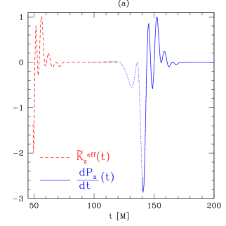
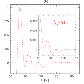
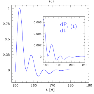
Figure 12: Effective curvature $\tilde{K}^{\mathrm{eff}}_{z}$ defined at the horizon via Eq. (37) (red dashed curve) and flux of momentum $(dP_{z}^{\cal B}/dt)$ evaluated at an approximation of ${I}^{+}$ with Eq. (33) (blue dotted and solid curves). These quantities encode, respectively, the information of the common horizon deformation and the flux of momentum carried away by GWs in the head-on collision of BHs with mass ratio 1/2. Note, at panel (a), the qualitative agreement between those curves, which allows us to distinguish the momentum radiated before (blue dotted curve) and after (blue solid curve) the merge. Panel (b) and (c) compares the same quantities for latter times, where one can still see the good agreement.

Note that one should not expect a perfect match between $(dP_{z}^{\cal B}/dt)(t)$ at ${I}^{+}$ and $\tilde{K}^{\mathrm{eff}}_{z}(t)$ at ${\cal H}^{+}$, even if the latter results to be a good estimator of the former. Indeed, (nonlinear) gravitational dynamics in the bulk spacetime affect and distort the possible relation between both quantities. Furthermore, given the related but different nature of ${}^{2}\!R$ and $\Psi_{4}$ it is not obvious that a correlation should be found at all.

In order to assess the validity of the approach, we construct $\tilde{K}^{\mathrm{eff}}_{z}(t)$ and $(dP_{z}^{\cal B}/dt)(t)$ from the numerical simulations described in Sec. IV.1. Note that because $\tilde{I}_{1}$ vanishes identically, the contributions $\tilde{\cal N}_{0}\tilde{\cal N}_{1}$ and $\tilde{\cal N}_{1}\tilde{\cal N}_{2}$ are absent in the expression for $\tilde{K}^{\mathrm{eff}}_{z}(t)$. Furthermore, since higher-order multipoles $\tilde{I}_{\ell}$ become increasingly difficult to calculate, we truncate expression (41) at $\ell=6$; in our case, this has little influence on the overall results as we will show that the lowest (i.e., $\ell=2,3$) modes are by large the dominant ones.

The values for $(dP_{z}^{\cal B}/dt)$ and $\tilde{K}^{\mathrm{eff}}_{z}$ as functions of the time $t$, and corresponding to the numerical simulations described in the previous Sec. IV.1, are presented in Fig. 12. The signals have been normalized with respect to their maximum value [a global rescaling does not affect the cross-correlations properties of two functions $h_{1}(t)$ and $h_{2}(t)$, cf. Appendix A]. In Fig. 12 (a), the quantity $\tilde{K}^{\mathrm{eff}}_{z}$ is shown from the time $t_{c}\approx 49.2M$ of first appearance of the common horizon (red dashed line). After time $t_{\mathrm{max}}\approx 120M$ the error in the calculation of the $\tilde{I}_{\ell}$ multipoles becomes comparable with the value of the multipoles, spoiling the evaluation of the integrals in (40). Hence, we set $\tilde{K}^{\mathrm{eff}}_{z}$ to zero for $t>t_{\mathrm{max}}$. Similarly, the flux of Bondi linear momentum $(dP_{z}^{\cal B}/dt)$ as computed by an observer at $100\,M$ from the origin, is split in a part before the appearance of the common AH (blue dotted line) and in one which is to be compared with $\tilde{K}^{\mathrm{eff}}_{z}$ (blue dashed line). In panels (b) and (c) of Fig. 12 we show instead $\tilde{K}^{\mathrm{eff}}_{z}$ and $(dP_{z}^{\cal B}/dt)$ separately and in different time intervals for a better emphasis of the similarities.

Some interesting remarks on Fig. 12 can be made already at a qualitative level. In particular, it is clear that $\tilde{K}^{\mathrm{eff}}_{z}$ succeeds in tracking key features of $(dP_{z}^{\cal B}/dt)$. This is apparent in the relative magnitude of the three first positive peaks in the two signals and the qualitative agreement is maintained in time. As expected, some specific features of $(dP_{z}^{\cal B}/dt)$ are not faithfully captured in $\tilde{K}^{\mathrm{eff}}_{z}$, such as the magnitude of the negative peak around $t\approx 148M$ relative to the neighboring peaks. However given the heuristic character of $\tilde{K}^{\mathrm{eff}}_{z}$ and the fact that its geometric definition does not leave room for any tuning, the overall qualitative agreement with $(dP_{z}^{\cal B}/dt)$ at ${I}^{+}$ already represents a remarkable result, shedding light on the near-horizon dynamics. This agreement between $(dP_{z}^{\cal B}/dt)$ and $\tilde{K}^{\mathrm{eff}}_{z}$ is indeed the main result of this section and the ultimate justification for the introduction of $\tilde{K}^{\mathrm{eff}}_{z}$. It is also worth stressing that attempts employing other quantities (e.g. a blind application of the methods used for RT spacetimes) would not lead to such a clear matching.

From a quantitative point of view, the correlation analysis for the time intervals shown in Fig. 12 (b) and (c) indicates that the two signals yield a typical correlation ${\cal M}\approx 0.93$ and a time lag $\tau=97M$ (we recall that the observer is at $100\,M$ and that the common AH has the size of a couple of $M$). However, as one tries to extend the analysis to the very first time of the formation of the apparent horizon, the correlation drops significantly. The reason for this drop is related to the stretching of the time coordinate between the two screens. In addition to the obvious time delay between the $(dP_{z}^{\cal B}/dt)(t)$ and $\tilde{K}^{\mathrm{eff}}_{z}(t)$ due to the finite (coordinate) speed of light, in fact, the dependence of the two signals in coordinate time $t$ is not the same and is stretched between the two screens. This effect is the result of the in-built gauge mapping between sections of ${I}^{+}$ and the horizon ${\cal H}^{+}$ defined by the spacetime slicing, but also of the physical blueshift (redshift) of signals at the inner (outer) boundaries in the BH spacetime.

Although approaches to disentangle the physical and gauge contributions can be derived, for instance by introducing proper times of suitably defined observers, this goes beyond the scope of this paper. Rather, we opt here for a more straightforward approach in which only comparisons based on sequences of (absolute values and signs of the) maxima and minima in the signals $h_{\mathrm{inn}}(t)$ and $h_{\mathrm{out}}(t)$ are considered significant, since the relative shape of $h_{\mathrm{inn}}(t)$ and $h_{\mathrm{out}}(t)$ can be subject to a time reparametrization. This association is possible when the quantities which are compared are scalars, so that the values of maxima and minima are well-defined and independent of coordinates. This is possible in the case of axisymmetry as it gives a privileged direction along which to contract the effective-curvature vector $\tilde{K}^{\mathrm{eff}}_{i}$. In a more generic configuration one would need to build an appropriate frame to produce scalars by contraction with tensorial quantities. Once the correspondence between maxima and minima in the two signals $h_{\mathrm{inn}}(t)$ and $h_{\mathrm{out}}(t)$ is established, a mapping $t_{\mathrm{out}}=t_{\mathrm{out}}(t_{\mathrm{inn}})$ can be easily constructed. With this matching, the calculation of the correlation parameter gives typically values ${\cal M}\geqslant 0.9$ for any chosen time interval . More information about the mapping between $t_{\mathrm{out}}$ and $t_{\mathrm{in}}$ is found in Appendix B.

IV.3.1 A critical assessment of the correlation

Of course, it is reasonable to question if finding such a high correlation is just a bias in our methodology. Certainly, our strategy of identification of maxima and minima in the signals enhances the correlations when time-stretching issues are involved. However, it does not guarantee by itself the high (positive) values found for ${\cal M}$. More specifically, once a first couple of maxima (or minima) are identified in the two signals, the subsequent couples of maxima and minima constructed from the data in each signal are automatically fixed. As a consequence, high correlations are possible only if the sequence of signs in the extrema of the two signals is exactly the same. In addition to consideration above, one may also argue that the high correlation found is just the result of the very rapid decay of the signals, which makes the first couple of maxima and minima play a dominant role in the estimate, possibly shadowing the role of the smaller peaks appearing at later times. To address this point and weight equally all parts of the signals, we model them as exponentially decaying oscillating functions, i.e., $h^{\kappa}_{\mathrm{inn}}(t)\equiv e^{\kappa_{\mathrm{inn}}t}h_{\mathrm{inn}}(t)$ and $h^{\kappa}_{\mathrm{out}}(t)\equiv e^{\kappa_{\mathrm{out}}t}h_{\mathrm{out}}(t)$. This is applied to the signals without the time correction provided by the map $t_{\rm out}=t_{\rm out}(t_{\rm inn})$ , finding

$$M\kappa_{\mathrm{inn}}=0.179\pm 0.005\,,\qquad M\kappa_{\mathrm{out}}=0.181\pm 0.006\ ,$$ (53)

through a least-square fitting. The resulting functions $h^{\kappa}_{\mathrm{inn}}(t)$ and $h^{\kappa}_{\mathrm{out}}(t)$ once the exponential decay has been subtracted are shown in Fig. 13. Once again it is apparent that the two time series are very similar and indeed the matching computed even without introducing any time mapping is ${\cal M}(h^{\kappa}_{\mathrm{inn}},h^{\kappa}_{\mathrm{out}})=0.87$ and thus remarkably high.

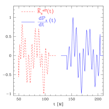
Figure 13: Quantities on ${\cal H}^{+}$ (red dashed line) and ${I}^{+}$ (blue solid line) as shown in Fig. 12 but without an overall exponential decay in time. The close similarity in the signals is confirmed by the very large correlation which is ${\cal M}=0.87$, obtained without a time mapping.

The main reason behind the good correlation found also for the undamped signals is that the next-to-leading-order term, i.e., term $\tilde{\cal N}_{3}\tilde{\cal N}_{4}$ and the corresponding $\ell=3$ and $\ell=4$ coupling in Eq. (50), are much smaller than the leading-order term ${\cal N}_{2}{\cal N}_{3}$. Indeed, we have found that it is possible to express to a very good approximation $\tilde{K}^{\mathrm{eff}}_{z}\sim\tilde{\cal N}_{2}\tilde{\cal N}_{3}$ and $(dP_{z}^{\cal B}/dt)\sim{\cal N}_{2}{\cal N}_{3}$. This is confirmed by the corresponding power spectra, which are shown in Fig. 14 and are dominated in both cases by two frequencies: $\Omega^{\mathrm{inn}}_{1}=0.22\pm 0.04,\,\Omega^{\mathrm{inn}}_{2}=0.98\pm 0.05$ for the signal $h_{\mathrm{inn}}(t)$, and $\Omega^{\mathrm{out}}_{1}=0.22\pm 0.04,\,\Omega^{\mathrm{out}}_{2}=0.97\pm 0.04$ for the signal $h_{\mathrm{out}}(t)$.

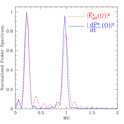
Figure 14: Normalized power spectrum for $K_{z}^{\rm eff}(\Omega)$ (red dashed line) and $(dP_{z}/dt)(\Omega)$ (blue solid line) as measured at ${\cal H}^{+}$ and ${I}^{+}$, respectively (cf. Figure 13). Both spectra are dominated by two frequencies: $\Omega^{\mathrm{inn}}_{1}=0.22\pm 0.04$ and $\Omega^{\mathrm{inn}}_{2}=0.98\pm 0.05$ (red dashed line) and $\Omega^{\mathrm{out}}_{1}=0.22\pm 0.04$ and $\Omega^{\mathrm{out}}_{2}=0.97\pm 0.04$ (blue solid line) which are linear combinations of the quasinormal ringing modes of the merged BH (cf. Table 1).

These frequencies are closely related to the quasinormal modes of the merged BH, interfering to lead to a beating signal. To see this, we model each function $\tilde{\cal N}_{\ell}$ and ${\cal N}_{\ell}$ as an exponentially damped sinusoid, i.e., $\tilde{\cal N}_{\ell}\sim e^{-\kappa^{\tilde{\cal N}}_{\ell}t}\mathrm{\sin}(\Omega^{\tilde{\cal N}}_{\ell}t+\varphi^{\tilde{\cal N}})$ and ${\cal N}_{\ell}\sim e^{-\kappa^{{\cal N}}_{\ell}t}\mathrm{\sin}(\Omega^{{\cal N}}_{\ell}t+\varphi^{\cal N})$. Then, under the approximation $\tilde{K}^{\mathrm{eff}}_{z}\sim\tilde{\cal N}_{2}\tilde{\cal N}_{3}$ and $(dP_{z}^{\cal B}/dt)\sim{\cal N}_{2}{\cal N}_{3}$ it follows

$$\Omega^{\tilde{\cal N}}_{\ell=2}=\frac{\Omega^{\mathrm{inn}}_{2}-\Omega^{\mathrm{inn}}_{1}}{2}\,,\quad\Omega^{\tilde{\cal N}}_{\ell=3}=\frac{\Omega^{\mathrm{inn}}_{2}+\Omega^{\mathrm{inn}}_{1}}{2}\,,$$ (54)

at ${\cal H}^{+}$, whereas

$$\Omega^{\cal N}_{\ell=2}=\frac{\Omega^{\mathrm{out}}_{2}-\Omega^{\mathrm{out}}_{1}}{2}\,,\quad\Omega^{\cal N}_{\ell=3}=\frac{\Omega^{\mathrm{out}}_{2}+\Omega^{\mathrm{out}}_{1}}{2}\,,$$ (55)

at ${I}^{+}$, consistent with the “beating” behavior shown by the power spectra in Fig. 14. Similarly, the decay time scales are then given by

$$\kappa_{\mathrm{inn}}=\kappa^{\tilde{\cal N}}_{\ell=2}+\kappa^{\tilde{\cal N}}_{\ell=3}\ \ ,\ \ \kappa_{\mathrm{out}}=\kappa^{{\cal N}}_{\ell=2}+\kappa^{{\cal N}}_{\ell=3}.$$ (56)

These frequencies and time scales match very well the real $(\omega^{\rm R}_{\ell})$ and imaginary $(\omega^{\rm I}_{\ell})$ parts of the fundamental $(n=0)$ quasi-normal-modes (QNM) eigenfrequencies of a Schwarzschild BH Berti et al. (2009). A detailed comparison is presented in Table 1, whose first six columns report the properties of the signals $h_{\mathrm{inn}}(t)$ and $h_{\mathrm{out}}(t)$ in their constituent frequencies $\Omega^{\cal N}_{\ell=2,3}$ and $\Omega^{\tilde{\cal N}}_{\ell=2,3}$ defined in Eqs. (54)–(55), and compare them with the corresponding real parts of the eigenfrequencies of a Schwarzschild BH, $\omega^{\rm R}_{\ell=2,3}$. The close match in the oscillatory part is accompanied also by a very good correspondence in the decaying part of the signal. Defining, in fact, the overall decay time in terms of the imaginary parts of the QNM eigenfrequencies, i.e., as $\kappa_{\mathrm{decay}}\equiv\omega_{\rm I}^{\ell=2}+\omega_{\rm I}^{\ell=3}$, it is easy to realize from the last three columns in Table 1, that this decay time is indeed very close to the one associated to the signal at the two screens [cf. Equations (55) and (56)].

This role of QNMs is not entirely surprising for a measure at ${I}^{+}$, but it is far less obvious to see it imprinted also for a quantity measured at ${\cal H}^{+}$. This indicates that the bulk spacetime dynamics responsible for the recoil physics is a relatively mild one, so that a QNM ringdown behavior dominates the dynamics of the deformed single AH and imprints the properties of the radiated linear momentum. It is interesting that a purely (quasi-)local study of the AH geometric properties permits us to read the behavior of quantities which are intrinsically defined at infinity, thus confirming the main thesis in Ref. Rezzolla et al. (2010).

Table 1: The first six columns offer a comparison between the properties of the signals $h_{\mathrm{inn}}(t)$ and $h_{\mathrm{out}}(t)$ in their constituent frequencies $\Omega^{\cal N}_{\ell=2,3}$ defined in Eqs. (54)–(55), with the corresponding real parts of the eigenfrequencies of a Schwarzschild BH, $\omega^{\rm R}_{\ell=2,3}$. The last three columns show instead a comparison between the damping times $\kappa_{\mathrm{inn,out}}$ defined in Eq. (56), with the corresponding decay time $\kappa_{\mathrm{decay}}$ computed from the imaginary parts of the eigenfrequencies. In all cases, the close match is remarkable and not at all obvious for quantities measured at ${\cal H}^{+}$.

$M\Omega^{\tilde{\cal N}}_{\ell=2}$	$M\Omega^{\cal N}_{\ell=2}$	$M\omega^{\rm R}_{\ell=2}$	$M\Omega^{\tilde{\cal N}}_{\ell=3}$	$M\Omega^{\cal N}_{\ell=3}$	$M\omega^{\rm R}_{\ell=3}$	$M\kappa_{\mathrm{inn}}$	$M\kappa_{\mathrm{out}}$	$M\kappa_{\mathrm{decay}}$
$0.38\pm 0.04$	$0.37\pm 0.04$	$0.37367$	$0.60\pm 0.04$	$0.59\pm 0.04$	$0.59944$	$0.181\pm 0.006$	$0.179\pm 0.005$	$0.18166$

IV.3.2 Antikicks and the Slowness Parameter

As a concluding remark for this section, we make use of our results, and, in particular, on the spectral and decaying properties of our measures on the screens, to make contact with the analysis carried out in Price et al. (2011). More specifically, we can define a characteristic decay time $\tau\equiv(2\pi)/\kappa^{\rm inn/out}$ and an oscillation-characteristic time $T\equiv 2\pi/\Omega^{\mathrm{inn/out}}_{2}$, from which to build our equivalent of the “slowness parameter” $P\equiv T/\tau$ introduced in Price et al. (2011). The specific case discussed above then yields $\tau\simeq 34.9M$, $T\simeq 6.4M$ and thus $P\simeq 0.18$. As detailed in Ref. Price et al. (2011), small antikicks should happen when the two timescales are comparable, thus corresponding to an oscillation which is over-damped. This expectation is indeed confirmed by the recoil velocity shown in Fig. 10, where the relative antikick is about $\sim 30\%$ and thus compatible with the slowness parameter that we have associated to our process [see also the discussion below on the application of Eqs. (57) and (58) in Fig. 15]. This qualitative agreement with the phenomenological approach discussed in Ref. Price et al. (2011) is very natural. While we here concentrate on modeling the local curvature properties at the horizon, Ref. Price et al. (2011) concentrates on the spectral features of the signal at large distances. Since we have demonstrated that the two are highly correlated, it does not come as a surprise that the two approaches are compatible. Looking at the local horizon’s properties has however the added value that it provides a precise framework in which to predict not only the strength of the antikick, but also its directionality. Furthermore, such an approach permits an interpretation of BH dynamics in terms of viscous hydrodynamics, as we will discuss in detail in paper II. In particular, we shall show there that the horizon-viscous analogy naturally leads to a geometric prescription for an (instantaneous) slowness parameter $P$, in terms of timescales $\tau$ and $T$ respectively related to bulk and shear viscosities.

The logic developed above for the calculation of the slowness parameter can be brought a step further by assuming that the final BH produced by the merger of a binary system in quasicircular orbit can be described at the lowest order by an oscillation and decay times

$$\tau \equiv \frac{2\pi}{\omega_{\ell=2}^{\textrm{I}}+\omega_{\ell=3}^{\textrm{I}}}\,,\qquad T\equiv\frac{2\pi}{\omega_{\ell=2}^{\textrm{R}}+\omega_{\ell=3}^{\textrm{R}}}\,,$$ (57)

to which corresponds a slowness parameter defined as

$$P \equiv \frac{T}{\tau}=\frac{\omega_{\ell=2}^{\textrm{I}}+\omega_{\ell=3}^{\textrm{I}}}{\omega_{\ell=2}^{\textrm{R}}+\omega_{\ell=3}^{\textrm{R}}}\,.$$ (58)

Using the semianalytic expressions derived for estimating the spin of the final BH, e.g.  Rezzolla et al. (2008a, b); Barausse and Rezzolla (2009), it is possible to predict the values of $\tau$ and $T$ for any binary whose initial spins and masses are known, and thus predict qualitatively through $P$ the strength of the antikick which will be produced in any of these configurations. We have tested this idea by considering the data presented in Ref. Pollney et al. (2007) both for the kick/antikick velocities and for the final spin of the merged BH. This conjecture about the predictability of the antikick in terms of the slowness parameter is indeed supported by the example data collected in Fig. 15. More specifically, the left panel in Fig. 15 shows the correlation between the slowness parameter $P=T/\tau$ as computed in Eq. (58) and the dimensionless spin of a BH $\tilde{a}_{\textrm{fin}}=J_{\textrm{fin}}/M_{\textrm{fin}}^{2}$ produced, for example, in the merger of a binary system (expressions to estimate the QNM eigenfrequencies for rotating BHs can be found in a number of works which are collected in the review Berti et al. (2009)). The middle panel shows instead the good correlation between the relative antikick velocity $\Delta v/v_{\textrm{fin}}\equiv(v_{\textrm{max}}-v_{\textrm{fin}})/v_{\textrm{fin}}=v_{\textrm{k}}/v_{\textrm{fin}}$ and the dimensionless final spin as computed from the data taken from Ref. Pollney et al. (2007) (indicated with error bars are the estimated numerical errors). Finally, the right panel combines the first two and shows the searched correlation between the antikick velocity and the slowness parameter. It also shows with a solid line an exponential fit, which suggests a vanishing antikick for a slowness parameter $P\sim 1$. All in all, this figure confirms also for the case of binaries in quasicircular orbits the suggestion Price et al. (2011) that the smaller the slowness parameter $P$ gets, the larger is the expected value of the antikick. Large antikicks should then be expected for $P\ll 1$ Price et al. (2011). Furthermore, it highlights that it is indeed possible to predict qualitatively the antikick merely on the basis of the initial properties of the BHs when the binary is still widely separated.

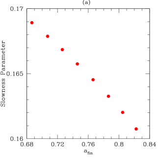
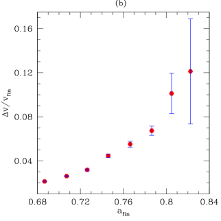
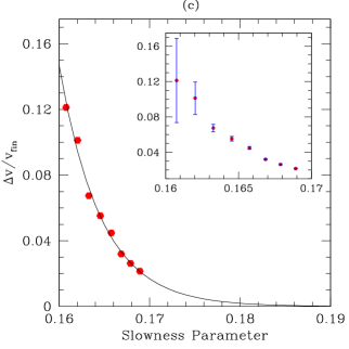
Figure 15: Predictability of the antikick in terms of the slowness parameter and the antikick. The left panel shows the correlation between the slowness parameter $P=T/\tau$ as computed in Eq. (58) and the dimensionless spin of a BH $a_{\textrm{fin}}$. The mid panel shows instead the good correlation between the relative antikick velocity $\Delta v/v_{\textrm{fin}}=v_{\textrm{k}}/v_{\textrm{fin}}$ and the dimensionless final spin, using the data taken from Ref. Pollney et al. (2007) (indicated with error bars are the estimated numerical errors). Finally, the right panel combines the first two and shows the correlation between the antikick velocity and the slowness parameter. In particular, the good exponential fitting shows the consistency with a vanishing antikick for a slowness parameter $P\sim 1$, as discussed in Price et al. (2011).

V Conclusions

We have demonstrated that qualitative aspects of the post-merger recoil dynamics at infinity can be understood in terms of the evolution of the geometry of the common horizon of the resulting black hole. This extends to binary black-hole spacetimes the conclusions presented in Ref. Rezzolla et al. (2010) based on Robinson-Trautman spacetimes. More importantly, we have shown that suitably built quantities defined on inner and outer world tubes (represented either by dynamical horizons or by timelike boundaries) can act as test screens responding to the spacetime geometry in the bulk, thus opening the way to a cross-correlation approach to probe the dynamics of spacetime.

The extension presented here is nontrivial and it involves the construction of a phenomenological vector $\tilde{K}^{\mathrm{eff}}_{i}(t)$ from the Ricci curvature scalar ${}^{2}\!R$ on the dynamical-horizon sections, which then captures the global properties of the flux of Bondi linear momentum $(dP_{i}^{\mathrm{B}}/dt)(t)$ at infinity, namely, (proportional to) the acceleration of the BH. At the same time, the proposed approach involves the development of a cross-correlation methodology which is able to compensate for the in-built gauge character of the time evolution on the two surfaces. A proper mapping between the times on the two surfaces is needed and its gauge nature highlights that the physical information encoded in the surface quantities is not in its local (arbitrary) time dependence, but rather in the global structure of successive maxima and minima.

By analyzing Robinson-Trautman spacetimes, Ref. Rezzolla et al. (2010) proposed that when a single horizon is formed during the merger of two BHs, the observed decelerations/accelerations of the newly formed BH can be understood in terms of the dissipation of an anisotropic distribution of the Ricci scalar curvature on the horizon. The results presented here confirm this picture, although through quantities which are suited to BH spacetimes. Being computed on the horizon, these quantities reflect the properties of the BH and, in particular, its exponentially damped ringing. The interplay between oscillation and decay timescales associated with this process, which are inevitably imprinted in our geometric variables, explain the late qualitative features of the recoil dynamics, in particular, the antikick, in natural connection with the approach discussed in Ref. Price et al. (2011), where the antikick is explained in terms of the spectral features of the signal at large distances. Because we have shown that the latter is closely correlated with the signal at the horizon, we can adopt the same slowness parameter introduced in Ref. Price et al. (2011) to predict qualitatively the magnitude of the antikick from the merger of BH binaries with spin aligned to the orbital angular momentum, finding a very good agreement with the numerical data.

As a final remark we note that looking at the horizon’s properties has the added value that it provides a precise framework in which to predict not only the strength of the antikick, but also its directionality. Furthermore, as we discuss in detail in paper II, our geometric (cross-correlation) framework presents a number of close connections with (and potential implications on) the literature developing around the use of horizons to study the dynamics of BHs, as well as with the interpretations of such dynamics in terms of a viscous hydrodynamics analogy. Much of the machinery developed using dynamical trapping horizons as inner screens can be extended also when a common horizon is not formed (as in the calculations reported in Ref. Sperhake et al. (2011)). While in such cases the identification of an appropriate hypersurface for the inner screen can be considerably more difficult, once this is found its geometrical properties can be used along the lines of the cross-correlation approach discussed here for dynamical horizons.

Appendix A Correlation and matching of time series

The correlation function ${\cal C}(h_{1},h_{2};\tau)$ introduced in Sec. IV.3 provides information in the time domain about the comparison of temporal series $h_{1}(t)$ and $h_{2}(t)$. Its Fourier transform defines the cross-spectrum${\cal C}(h_{1},h_{2};f)$ of $h_{1}$ and $h_{2}$, providing the corresponding analysis in the frequency domain. It has the form

$${\cal C}(h_{1},h_{2};f)=\tilde{h}_{1}(f)\tilde{h}_{2}^{*}(f)\,,$$ (59)

where Fourier transform conventions are

$$\tilde{h}_{i}(f)=\int_{-\infty}^{\infty}h_{i}(t)e^{i2\pi ft}dt\ \,,\ \ h_{i}(t)=\int_{-\infty}^{\infty}\tilde{h}_{i}(f)e^{-i2\pi ft}df\,.$$ (60)

Choosing a measure $(S_{n}(|f|))^{-1}df$, a natural scalar product between functions $h_{1}(t)$ and $h_{2}(t)$ (or $\tilde{h}_{1}(f)$ and $\tilde{h}_{2}(f)$) is introduced as

$$\langle h_{1},h_{2}\rangle=\int_{-\infty}^{\infty}\frac{\tilde{h}_{1}(f)\tilde{h}_{2}^{*}(f)}{S_{n}(|f|)}df.$$ (61)

In GW data analysis $S_{n}(|f|)$, the noise power-spectral density, is associated with the spectral sensitivity of the instrument. In our case we have no a priori knowledge about $S_{n}(|f|)$, and we choose $S_{n}(f)=1$. The scalar product $\langle\cdot,\cdot\rangle$ introduces the natural projection between $\tilde{h}_{1}(f)$ and $\tilde{h}_{2}(f)$. Their normalized scalar product defines the overlap

$${\cal O}[h_{1},h_{2}]\equiv\frac{\langle h_{1},h_{2}\rangle}{\sqrt{\langle h_{1},h_{1}\rangle\langle h_{2},h_{2}\rangle}}\,.$$ (62)

Fixing one of the functions, say $h_{1}(t)$, we can consider its overlap with the function resulting by shifting $h_{2}(t)$ in time by a time lag $\tau$, i.e., $h_{2}(t+\tau)$. In the frequency domain this amounts to calculate the overlap between $\tilde{h}_{1}(t)$ and $\tilde{h}_{2}(f,\tau)=\tilde{h}_{2}(f)e^{-i2\pi f\tau}$. Maximizing over $\tau$ provides the best match estimator

$${\cal M}(h_{1},h_{2}) \equiv \max\limits_{\tau}\{{\cal O}[h_{1},h_{2}(\tau)]\}=\max\limits_{\tau}\frac{\langle h_{1},h_{2}(\tau)\rangle}{\sqrt{\langle h_{1},h_{1}\rangle\langle h_{2},h_{2}\rangle}}$$

$$= \max\limits_{\tau}\frac{\int_{-\infty}^{\infty}\tilde{h}_{1}(f)\tilde{h}_{2}^{*}(f)e^{-i2\pi f\tau}df}{\left(\int_{-\infty}^{\infty}|\tilde{h}_{1}(f)|^{2}df\int_{-\infty}^{\infty}|\tilde{h}_{2}(f)|^{2}df\right)^{\frac{1}{2}}}\,.$$

We note that, according to expression (59), the numerator in the second line of Eq. (A) is the inverse Fourier transform of the cross-spectrum function ${\cal C}(h_{1},h_{2})(f)$. Therefore the numerator in the expression for ${\cal M}(h_{1},h_{2})$ is just the correlation function ${\cal C}(h_{1},h_{2})(\tau)$. Regarding the denominator, we use Parseval’s identity

$$\int_{-\infty}^{\infty}|\tilde{h}_{i}(f)|^{2}df=\int_{-\infty}^{\infty}|h_{i}(t)|^{2}dt,$$ (64)

and the expression for the autocorrelation of functions $h_{i}(t)$

$$\int_{-\infty}^{\infty}|h_{i}(t)|^{2}dt={\cal C}(h_{i},h_{i};\tau=0)\ \,.$$ (65)

We then recover expression (52) for ${\cal M}(h_{1},h_{2})$ in terms of the correlation function ${\cal C}(h_{1},h_{2};\tau)$.

Appendix B Mapping time series on the screens

As discussed in Sec. IV.3, a built-in gauge mapping between sections of ${I}^{+}$ and the horizon ${\cal H}^{+}$ defined by the spacetime slicing leads to a stretching of the time coordinate between the two screens.

A comparison based on sequences of maxima and minima in the signals $h_{\mathrm{inn}}(t)$ and $h_{\mathrm{out}}(t)$ allows us to construct the mapping $t_{\mathrm{out}}(t_{\mathrm{inn}})$, which is here depicted in Fig.16a. Also shown in Fig.16b is the derivative of this interpolation, crucial to assess the relative rate of the considered coordinate times. In particular, it addresses the behavior discussed in footnote (10).

Finally, Fig.16c presents the correlation number ${\cal M}$ between the two signals as a function of time intervals $\Delta$. The construction of the intervals $\Delta$ is based on the sequences of maxima and minima identified in the two signals. In this way, we fix the final time in both series as $t^{\rm final}_{\rm inn}=96.8M$ and $t^{\rm final}_{\rm out}=194.4M$ and then we establish windows $\Delta=t^{\rm final}-t^{\rm initial}$, starting from $t^{\rm initial}_{\rm inn}=49.2M$ and $t^{\rm initial}_{\rm out}=140.4M$. For the red curve, the correlation is evaluated without using the mapping $t_{\rm out}=t_{\rm out}(t_{\rm inn})$ to correct the stretching, while the black curve takes the effect into account. This latter figure shows that the correction through the mapping $t_{\rm out}=t_{\rm out}(t_{\rm inn})$ is crucial to disentangle coordinate from real effects at early times.

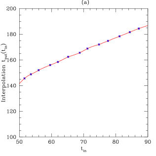
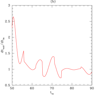
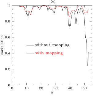
Figure 16: Mapping between the coordinate time $t_{\rm in}$ and $t_{\rm out}$ measured at the inner/outer screens. The first panel shows the interpolation of the function $t_{\rm out}=t_{\rm out}(t_{\rm in})$ constructed from the comparison between the sequence of maxima and minima in the signals $h_{\rm inn}(t)$ and $h_{\rm out}(t)$. The middle panel depicts the interpolation’s derivative $dt_{\rm out}/dt_{\rm in}$. In particular, it shows that initially the coordinate time at ${I}^{+}$ runs faster than the time at ${\cal H}^{+}$ and than oscillates around unity at late times. This behavior is consistent with the approach to stationarity. Finally, the right panel presents the correlation number ${\cal M}$ as a function of time intervals $\Delta$. The red curve shows the correlation without the using the mapping $t_{\rm out}=t_{\rm out}(t_{\rm in})$ to correct the time stretching between the signals on the two screens, whereas the black curve takes the effect into account and gives ${\cal M}\geqslant 0.9$. This correction is crucial to disentangle coordinate from real effects at early times.

References

- Rezzolla et al. (2010) L. Rezzolla, R. P. Macedo, and J. L. Jaramillo, Phys. Rev. Lett. 104, 221101 (2010).
- Jaramillo et al. (2012) J. L. Jaramillo, R. P. Macedo, P. Moesta, and L. Rezzolla, Phys. Rev. D 85, 084031 (2012).
- Peres (1962) A. Peres, Phys. Rev. 128, 2471 (1962).
- Bekenstein (1973) J. D. Bekenstein, Astrophys. J. 183, 657 (1973).
- Fitchett and Detweiler (1984) M. J. Fitchett and S. Detweiler, Mon. Not. R. Astron. Soc. 211, 933 (1984).
- Nakamura and Haugan (1983) T. Nakamura and M. P. Haugan, Astrophys. J. 269, 292 (1983).
- Favata et al. (2004) M. Favata, S. A. Hughes, and D. E. Holz, Astrophys. J. 607, L5 (2004).
- Wiseman (1992) A. G. Wiseman, Phys. Rev. D 46, 1517 (1992).
- Kidder (1995) L. E. Kidder, Phys. Rev. D 52, 821 (1995).
- Blanchet et al. (2005) L. Blanchet, M. S. S. Qusailah, and C. M. Will, Astrophys. J. 635, 508 (2005).
- Damour and Gopakumar (2006) T. Damour and A. Gopakumar, Phys. Rev. D 73, 124006 (2006).
- Andrade and Price (1997) Z. Andrade and R. H. Price, Phys. Rev. D 56, 6336 (1997).
- Sopuerta et al. (2006) C. F. Sopuerta, N. Yunes, and P. Laguna, Phys. Rev. D 74, 124010 (2006).
- Baker et al. (2006) J. G. Baker, J. Centrella, D.-I. Choi, M. Koppitz, J. van Meter, and M. C. Miller, Astrophys. J. 653, L93 (2006).
- Gonzalez et al. (2007a) J. A. Gonzalez, U. Sperhake, B. Bruegmann, M. Hannam, and S. Husa, Phys. Rev. Lett. 98, 091101 (2007a).
- Campanelli et al. (2007a) M. Campanelli, C. O. Lousto, Y. Zlochower, and D. Merritt, Phys. Rev. Lett. 98, 231102 (2007a).
- Herrmann et al. (2007) F. Herrmann, I. Hinder, D. Shoemaker, P. Laguna, and R. A. Matzner, Astrophys. J. 661, 430 (2007).
- Koppitz and al. (2007) M. Koppitz and al., Phys. Rev. Lett. 99, 041102 (2007).
- Lousto and Zlochower (2008) C. O. Lousto and Y. Zlochower, Phys. Rev. D 77, 044028 (2008).
- Pollney et al. (2007) D. Pollney et al., Phys. Rev. D 76, 124002 (2007).
- Healy et al. (2009) J. Healy et al., Phys. Rev. Lett. 102, 041101 (2009).
- Campanelli et al. (2007b) M. Campanelli, C. O. Lousto, Y. Zlochower, and D. Merritt, Astrophys. J. 659, L5 (2007b).
- Gonzalez et al. (2007b) J. A. Gonzalez, M. D. Hannam, U. Sperhake, B. Bruegmann, and S. Husa, Phys. Rev. Lett. 98, 231101 (2007b).
- Rezzolla (2009) L. Rezzolla, Class. Quant. Grav. 26, 094023 (2009).
- Zlochower et al. (2011) Y. Zlochower, M. Campanelli, and C. O. Lousto, Classical Quantum Gravity 28, 114015 (2011).
- Le Tiec et al. (2010) A. Le Tiec, L. Blanchet, and C. M. Will, Class. Quant. Grav. 27, 012001 (2010).
- Schnittman et al. (2008) J. D. Schnittman, A. Buonanno, J. R. van Meter, J. G. Baker, W. D. Boggs, J. Centrella, B. J. Kelly, and S. T. McWilliams, Phys. Rev. D 77, 044031 (2008).
- Mino and Brink (2008) Y. Mino and J. Brink, Phys. Rev. D 78, 124015 (2008).
- Nichols and Chen (2010) D. A. Nichols and Y. Chen, Phys. Rev. D 82, 104020 (2010).
- Hamerly and Chen (2011) R. Hamerly and Y. Chen, Phys. Rev. D 84, 124015 (2011).
- Sperhake et al. (2011) U. Sperhake, E. Berti, V. Cardoso, F. Pretorius, and N. Yunes, Phys. Rev. D 83, 024037 (2011).
- Price et al. (2011) R. H. Price, G. Khanna, and S. A. Hughes, Phys. Rev. D 83, 124002 (2011).
- Robinson and Trautman (1962) I. Robinson and A. Trautman, Proc. Roy. Soc. Lond. A265, 463 (1962).
- D. Kramer and Herlt (1980) M. M. D. Kramer, H. Stephani and E. Herlt, Exact Solutions of Einstein’s Field Equations (Cambridge University Press, Cambridge, 1980).
- Ashtekar et al. (2004) A. Ashtekar, J. Engle, T. Pawlowski, and C. Van Den Broeck, Class. Quant. Grav. 21, 2549 (2004).
- Schnetter et al. (2006) E. Schnetter, B. Krishnan, and F. Beyer, Phys. Rev. D 74, 024028 (2006).
- Tod (1983) K. Tod, Proc. R. Soc. London A388, 457 (1983).
- Singleton (1990) D. Singleton, Classical Quantum Gravity 7, 1333 (1990).
- Chrusciel (1991) P. T. Chrusciel, Commun. Math. Phys. 137, 289 (1991).
- Chrusciel (1992) P. T. Chrusciel, Proc. Roy. Soc. Lond. 436, 299 (1992).
- Gómez et al. (1997) R. Gómez, L. Lehner, P. Papadopoulos, and J. Winicour, Classical Quantum Gravity 14, 977 (1997).
- de Oliveira and Damiao Soares (2004) H. P. de Oliveira and I. Damiao Soares, Phys. Rev. D 70, 084041 (2004).
- Moreschi and Dain (1996) O. M. Moreschi and S. Dain, Phys. Rev. D 53, R1745 (1996).
- Moreschi et al. (2002) O. Moreschi, A. Perez, and L. Lehner, Phys. Rev. D 66, 104017 (2002).
- de Oliveira and Soares (2005) H. P. de Oliveira and I. D. a. Soares, Phys. Rev. D 71, 124034 (2005).
- de Oliveira and Rodrigues (2008) H. P. de Oliveira and E. L. Rodrigues, Class. Quant. Grav. 25, 205020 (2008).
- de Oliveira et al. (2008) H. P. de Oliveira, I. D. a. Soares, and E. V. Tonini, Phys. Rev. D 78, 044016 (2008).
- Aranha et al. (2008) R. F. Aranha, H. P. de Oliveira, I. Damiao Soares, and E. V. Tonini, Int. J. Mod. Phys. D 17, 2049 (2008).
- Macedo and Saa (2008) R. P. Macedo and A. Saa, Phys. Rev. D 78, 104025 (2008).
- Podolsky and Svitek (2009) J. Podolsky and O. Svitek, Phys. Rev. D 80, 124042 (2009).
- Aranha et al. (2010a) R. Aranha, I. Damiao Soares, and E. Tonini, Phys.Rev. D 81, 104005 (2010a).
- Aranha et al. (2010b) R. F. Aranha, I. D. Soares, and E. V. Tonini, Phys. Rev. D 82, 104033 (2010b).
- de Oliveira et al. (2011a) H. P. de Oliveira, E. L. Rodrigues, and J. E. F. Skea, Phys. Rev. D 84, 044007 (2011a).
- Svítek (2011) O. Svítek, Phys. Rev. D 84, 044027 (2011).
- Penrose (1973) R. Penrose, Ann. NY Acad. Sci. 224, 125 (1973).
- Tod (1989) K. Tod, Class. Quant. Grav. 6, 1159 (1989).
- Chow and Lun (1999) E. W. M. Chow and A. W. C. Lun, J. Austral. Math. Soc. Serv. B 41, 217 (1999).
- Hayward (1994) S. A. Hayward, Phys. Rev. D 49, 6467 (1994).
- Ashtekar and Krishnan (2003) A. Ashtekar and B. Krishnan, Phys. Rev. D 68, 104030 (2003).
- Ashtekar and Krishnan (2004) A. Ashtekar and B. Krishnan, Living Rev. Relativ. 7, 10 (2004).
- de Oliveira et al. (2011b) H. de Oliveira, E. Rodrigues, and I. Damiao Soares, Braz.J.Phys. 41, 314 (2011b).
- (62) “http://einsteintoolkit.org,” .
- Schnetter et al. (2004) E. Schnetter, S. H. Hawley, and I. Hawke, Classical Quantum Gravity 21, 1465 (2004).
- Thornburg (2004) J. Thornburg, Classical Quantum Gravity 21, 743 (2004).
- Dreyer et al. (2003) O. Dreyer, B. Krishnan, D. Shoemaker, and E. Schnetter, Phys. Rev. D 67, 024018 (2003).
- Pollney et al. (2009) D. Pollney, C. Reisswig, N. Dorband, E. Schnetter, and P. Diener, Phys. Rev. D 80, 121502 (2009).
- Alcubierre (2008) M. Alcubierre, Introduction to Numerical Relativity (Oxford University Press, Oxford, UK, 2008).
- Berti et al. (2009) E. Berti, V. Cardoso, and A. O. Starinets, Class. Quant. Grav. 26, 163001 (2009).
- Rezzolla et al. (2008a) L. Rezzolla, E. N. Dorband, C. Reisswig, P. Diener, D. Pollney, E. Schnetter, and B. Szilágyi, Astrophys. J. 679, 1422 (2008a).
- Rezzolla et al. (2008b) L. Rezzolla, P. Diener, E. N. Dorband, D. Pollney, C. Reisswig, E. Schnetter, and J. Seiler, Astrophys. J. 674, L29 (2008b).
- Barausse and Rezzolla (2009) E. Barausse and L. Rezzolla, Astrophys. J. Lett. 704, L40 (2009).