Geometry in the entanglement dynamics of the double Jaynes–Cummings model.

Abstract

We report on the geometric character of the entanglement dynamics of two pairs of qubits evolving according to the double Jaynes–Cummings model. We show that the entanglement dynamics for the initial states $|\psi_{0}\rangle=\cos\alpha|10\rangle+\sin\alpha|01\rangle$ and $|\phi_{0}\rangle=\cos\alpha|11\rangle+\sin\alpha|00\rangle$ cover 3–dimensional surfaces in the diagram $C_{ij}\,\mathrm{x}\,C_{ik}\,\mathrm{x}\,C_{il}$, where $C_{mn}$ stands for the concurrence between qubits $m$ and $n$, varying $0\leq\alpha\leq\pi/2$. In the first case projections of the surfaces on a diagram $C_{ij}\,\mathrm{x}\,C_{kl}$ are conics. In the second case curves can be more complex. We relate those conics with a measurable quantity, the predictability. We also derive inequalities limiting the sum of the squares of the concurrence of every bipartition and show that sudden death of entanglement is intimately connected to the size of the average radius of a hyper-sphere.

1 Introduction

The capacity of quantum systems to entangle is perhaps the most intriguing aspect of quantum mechanics and is a feature that distinguishes classical from quantum physics. In a seminal work, Einstein, Podolsky, and Rosen epr have brought this property to discussion and since then the subject has been investigated. Recently, pure bipartite interacting quantum systems have proven to be a very useful tool to explore entanglement dynamics and unveil several of the intriguing properties which govern quantum correlations exchange. Examples of such properties are the sudden (or asymptotic) disappearance of entanglement morte , the so called entanglement sudden birth nascimento , control of entanglement dynamics controle and entanglement distribution distribuicao1 , an important ingredient for quantum computation. Perhaps the best known and explored model is the Jaynes–Cummings Model (JCM) JCM , where several dynamical scenarios have been explored both with and without dissipation. An analogous model, the Tavis-Cummings model tc has also been used for similar purposes. The result obtained in these two contexts have enlightened entanglement disappearance in finite time morte1 ; morte2 ; morte3 , relations between purity, energy and entanglement energia ; energia1 , invariant entanglement distribuicao and general aspects of entanglement dynamics between partitions geral ; geral1 ; geral2 ; geral3 . In the present work we show that the entanglement dynamics of the Double Jaynes–Cummings Model (DJCM) morte1 exhibits geometric properties for the two classes of initial states we considered. The scenario is a pair of initially entangled non-interacting atoms $``A"$ and $``B"$, two cavities “$a$” and “$b$” which interact locally via the JCM and we use concurrence wootters2 to quantify entanglement between these parts. We show that, for initial atomic states belonging to the class $|\psi_{0}\rangle=\cos\alpha|10\rangle+\sin\alpha|01\rangle$, the relations between concurrences describe a conic in a diagram $C_{ij}\,\mathrm{x}\,C_{kl}$, with $ij\neq kl$ ( $ij$ being equal to $Aa$, $Ab$, $AB$, $ab$, $aB$ and $Bb$). On the other hand, if the initial atomic state belongs to the class $|\phi_{0}\rangle=\cos\alpha|11\rangle+\sin\alpha|00\rangle$, the geometric curve is not as simple. However, in all cases when a conic is found, the eccentricity can be written as a function of the absolute value of the average excitations in $A$, in other words: $\mathcal{P}_{0}=\Bigl{|}\mathrm{tr}\bigl{(}\sigma_{z}^{A}\rho_{0}\bigr{)}\Bigr{|}$. If the initial atomic state is $|\psi_{0}\rangle$, $\mathcal{P}_{0}$ gives the probability of the excitation being found in only one of the two bipartition $Aa$ or $Bb$. On the other hand, if the initial state is $|\phi_{0}\rangle$, $\mathcal{P}_{0}$ does not have the same interpretation. It is important to notice that $\mathcal{P}_{0}$ is the predictability which according to the complementarity relation between two qubits proposed in ref. bergou is related to the initial concurrence. We find that this geometric character can be extended for more dimensions. It is possible to define a hyper-surface over which the concurrence dynamics between every two pairs $i$ and $j$ defines a trajectory over or inside this hyper surface.

The present work is organized as follows: In section 2 we present the physical model and the time evolution for the two classes of states, $|\psi_{0}\rangle$ and $|\phi_{0}\rangle$ ; Next, in section 3, we determine the entanglement (quantified by concurrence), and we construct the diagram $C_{ij}\,\mathrm{x}\,C_{kl}$ showing that whenever a conic is found its eccentricity is related to the predictability as defined in bergou ; In the following section, we show the existence of an entanglement surface for the dynamics of the pairs of concurrences involving the same qubit and justify why curves of the diagrams $C_{ij}\,\mathrm{x}\,C_{kl}$ will be over that surface; In section 5 we find an inequality which describes the entanglement dynamics of all qubit pairs; In section 6 we present how decoherence affects some of the conics and we conclude in section 7.

2 The physical model

Consider a composite system of two identical two-level atoms (“$A$” e “$B$”) and two identical cavities (“$a$” e “$b$”). The atom “$A$” (“$B$”) interacts resonantly with the cavity “$a$” (“$b$”), respectively, via JCM JCM and the evolution of the system is governed by the Hamiltonian

$$H = \hbar\omega a^{\dagger}a+\hbar\omega b^{\dagger}b+\dfrac{\hbar\omega}{2}\sigma_{z}^{A}+\dfrac{\hbar\omega}{2}\sigma_{z}^{B}+$$ (1)

$$+g\bigl{(}a^{\dagger}\sigma_{-}^{A}+a\sigma_{+}^{A}\bigr{)}+g\bigl{(}b^{\dagger}\sigma_{-}^{B}+b\sigma_{+}^{B}\bigr{)},$$

where $a^{\dagger}$ ($b^{\dagger}$) and $a$ ($b$) are the creation and annihilation operators of the field inside cavity $a$ ($b$), respectively. The matrices $\sigma_{-}^{i}$, $\sigma_{+}^{i}$ and $\sigma_{z}^{i}$ are Pauli matrices of the i–th atom, with $i=A,B$. The cavities are resonant with the atoms, i. e. the frequency of the field inside each cavity is equal to the frequency of the atomic transition of the atoms’ internal levels.

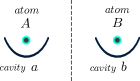
Figure 1: A schematic figure of the DJCM. In the left (right) partition there is the atom “$A$” (“$B$”) interacting with the cavity “$a$” (“$b$”), respectively, and there is no interaction between the partition “$Aa$” and “$Bb$”.

We consider the cavities initially in the vacuum state and some entanglement between the atoms. Consider the initial state of the system as

$$|\psi_{0}\rangle = (\cos\alpha|10\rangle+\sin\alpha|01\rangle)\otimes|00\rangle\ \ \ \ .$$ (2)

Because of the conservation of the number of excitations the time evolution can be determined analytically and it reads

$$|\psi_{t}\rangle = x_{1}(t)|10\rangle|00\rangle+x_{2}(t)|01\rangle|00\rangle+$$ (3)

$$+x_{3}(t)|00\rangle|10\rangle+x_{4}(t)|00\rangle|01\rangle\ \ \ \ .$$

The coefficients will be given by the Schrödinger equation, $i|\dot{\psi_{t}}\rangle=H|\psi_{t}\rangle$, plus the boundary conditions $x_{1}(0)=\cos\alpha$, $x_{2}(0)=\sin\alpha$, $x_{3}(0)=0$ and $x_{4}(0)=0$. They are

$$x_{1}(t) = \cos\alpha\cos(gt),$$ (4)

$$x_{2}(t) = \sin\alpha\cos(gt),$$ (5)

$$x_{3}(t) = -i\cos\alpha\sin(gt),$$ (6)

$$x_{4}(t) = -i\sin\alpha\sin(gt).$$ (7)

Consider also the initial state

$$|\phi_{0}\rangle = (\cos\alpha|11\rangle+\sin\alpha|00\rangle)\otimes|00\rangle\ \ \ \ .$$ (8)

The same thing can be done to find the time evolution. We have

$$|\phi_{t}\rangle = y_{1}(t)|11\rangle|00\rangle+y_{2}(t)|00\rangle|00\rangle+y_{3}(t)|10\rangle|01\rangle+$$ (9)

$$+y_{4}(t)|01\rangle|10\rangle+y_{5}(t)|00\rangle|11\rangle,\ \ \ \$$

where

$$y_{1}(t) = e^{-i\omega t}\cos\alpha\cos^{2}(gt),$$ (10)

$$y_{2}(t) = e^{i\omega t}\sin\alpha,$$ (11)

$$y_{3}(t) = -i\,e^{-i\omega t}\cos\alpha\sin(gt)\cos(gt),$$ (12)

$$y_{4}(t) = -i\,e^{-i\omega t}\cos\alpha\sin(gt)\cos(gt),$$ (13)

$$y_{5}(t) = -e^{-i\omega t}\cos\alpha\sin^{2}(gt)\ \ \ \ .$$ (14)

We can observe that, at time $t$ immediately after $t=0$, the state (3) and (9) will develop entanglement among all the partitions. However, we will consider the entanglement between qubits ($A$, $B$, $a$ e $b$) and their relations. Thus, we will use as entanglement quantifier the concurrence wootters2 , which is defined as

$$C=\max\Bigl{[}\,0\,,\sqrt{\lambda_{1}}-\sqrt{\lambda_{2}}-\sqrt{\lambda_{3}}-\sqrt{\lambda_{4}}\,\Bigr{]},$$ (15)

where $\lambda_{i}$ are the eigenvalues, organized in a descending order, of the matrix $\rho(\sigma_{y}\otimes\sigma_{y})\rho^{*}(\sigma_{y}\otimes\sigma_{y})$.

3 Entanglement dynamics in the diagram $C_{ij}\,\mathrm{x}\,C_{kl}$

We can easily find the state $\rho_{ij}$ of two qubits taking a partial trace over the remaining subsystem. We next determine all $C_{ij}$.

3.1 For the initial state $|\psi_{0}\rangle$

In this case we obtain

$$C_{AB} = |\sin 2\alpha|\cos^{2}(gt),$$ (16)

$$C_{ab} = |\sin 2\alpha|\sin^{2}(gt),$$ (17)

$$C_{Aa} = \cos^{2}\alpha|\sin(2gt)|,$$ (18)

$$C_{Ab} = |\sin 2\alpha\sin(gt)\cos(gt)|,$$ (19)

$$C_{aB} = |\sin 2\alpha\sin(gt)\cos(gt)|,$$ (20)

$$C_{Bb} = \sin^{2}\alpha|\sin(2gt)|\ \ \ \ .$$ (21)

We analyze the geometric structure of entanglement dynamics in a diagram $C_{ij}\,\mathrm{x}\,C_{kl}$. In order to do this, observe that we can sum eq.(16) with eq.(17) and we have

$$C_{AB}+C_{ab}=C_{0},$$ (22)

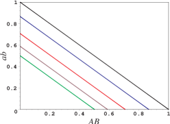
Figure 2: Graphic of the straight lines $C_{AB}\,\mathrm{x}\,C_{ab}$ with $\alpha=\pi/4,\pi/6,\pi/8,\pi/10\ \mathrm{and}\ \pi/12$ for the colors black, blue, red, brown and green, respectively.

where $C_{0}=|\sin 2\alpha|$ is the initial concurrence between the atoms $A$ and $B$. We notice that this equation defines a straight line in a diagram $C_{AB}\,\mathrm{x}\,C_{ab}$ (see figure 2). The lines in equation (22), when $\alpha\in(0,\pi/2)$, fill the triangle formed by the axis $C_{AB}$, $C_{ab}$ and $C_{AB}+C_{ab}=1$. In addition, we notice that equations (19) and (20) satisfy

$$C_{Ab}=C_{aB}.$$ (23)

This shows a symmetry between the cavity of one of the systems and the atom of the other. We proceed dividing (18) by (21) and we easily find

$$C_{Aa}=\dfrac{\cos^{2}\alpha}{\sin^{2}\alpha}C_{Bb},\ \ \ \$$ (24)

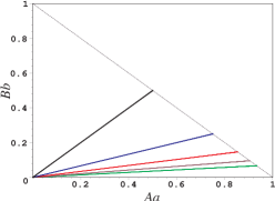
Figure 3: Graphic of the straight line $C_{Aa}\,\mathrm{x}\,C_{Bb}$ with $\alpha=\pi/4,\pi/6,\pi/8,\pi/10\ \mathrm{and}\ \pi/12$ for the colors black, blue, red, brown and green, respectively. The slim violet curve is the straight line $C_{Aa}+C_{Bb}=1$.

which is a straight line in the diagram $C_{Aa}\,\mathrm{x}\,C_{Bb}$. In the interval $0<\alpha<\pi/2$, the lines (24) are limited in the region between the lines $C_{Aa}=0$, $C_{Bb}=0$ and $C_{Aa}+C_{Bb}=1$. Equations (22 – 24) define a straight line in their respective diagram $C_{ij}\,\mathrm{x}\,C_{kl}$. The line $C_{Aa}+C_{Bb}=1$, which represents a conservation of entanglement, is a superior limit in all cases. Using the same procedure, and some simplifications, we find other conics (ellipses, circumferences and straight lines) which we organize as follows:

3.1.1 Concurrence between atoms (or cavities) versus concurrence between one of the atoms and its cavity:

• $C_{AB(ab)}\,\mathrm{x}\,C_{Bb}$:

  $$\dfrac{\bigl{(}C_{AB(ab)}-C_{0}/2\bigr{)}^{2}}{C_{0}^{2}/4}+\dfrac{C_{Bb}^{2}}{\sin^{4}\alpha}=1$$ (25)

  

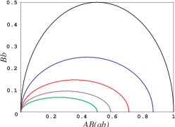
  Figure 4: Graphic of the semi–ellipse $C_{AB(ab)}\,\mathrm{x}\,C_{Bb}$ with $\alpha=\pi/4,\pi/6,\pi/8,\pi/10\ \mathrm{and}\ \pi/12$ for the colors black, blue, red, brown and green, respectively.

• $C_{AB(ab)}\,\mathrm{x}\,C_{Aa}$:

  $$\dfrac{\bigl{(}C_{AB(ab)}-C_{0}/2\bigr{)}^{2}}{C_{0}^{2}/4}+\dfrac{C_{Aa}^{2}}{\cos^{4}\alpha}=1$$ (26)

  

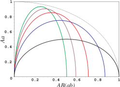
  Figure 5: Graphic of the semi–ellipse $C_{AB(ab)}\,\mathrm{x}\,C_{Aa}$ with $\alpha=\pi/4,\pi/6,\pi/8,\pi/10\ \mathrm{and}\ \pi/12$ for the colors black, blue, red, brown and green, respectively. The slim violet curve is the semi circumference $C_{AB(ab)}^{2}+C_{Aa}^{2}=1$.

3.1.2 Concurrence between atoms (or cavities) versus concurrence between one of the atoms and the cavity which does not contain it:

$$\bigl{(}C_{AB(ab)}-C_{0}/2\bigr{)}^{2}+\bigl{(}C_{aB(Ab)}\bigr{)}^{2}=C_{0}^{2}/4$$ (27)

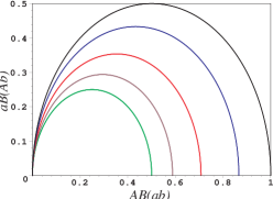
Figure 6: Graphic of the semi circumference $C_{AB(ab)}\,\mathrm{x}\,C_{aB(Ab)}$ with $\alpha=\pi/4,\pi/6,\pi/8,\pi/10\ \mathrm{and}\ \pi/12$ for the colors black, blue, red, brown and green, respectively.

3.1.3 Concurrence between one of the atoms and the cavity which does not contain it versus concurrence between one of the atoms and its cavity:

• $C_{aB(Ab)}\,\mathrm{x}\,C_{Aa}$:

  $$C_{aB(Ab)}=\dfrac{|\sin 2\alpha|}{2\cos^{2}\alpha}C_{Aa}$$ (28)

  

  Figure 7: Graphic of the straight line $C_{aB(Ab)}\,\mathrm{x}\,C_{Aa}$ with $\alpha=\pi/4,\pi/6,\pi/8,\pi/10\ \mathrm{and}\ \pi/12$ for the colors black, blue, red, brown and green, respectively. The slim violet curve is the semi circumference $(2C_{Aa}-1)^{2}+(2C_{aB(Ab)})^{2}=1$.

• $C_{Ab(aB)}\,\mathrm{x}\,C_{Bb}$:

  $$C_{Ab(aB)}=\dfrac{|\sin 2\alpha|}{2\sin^{2}\alpha}C_{Bb}$$ (29)

  

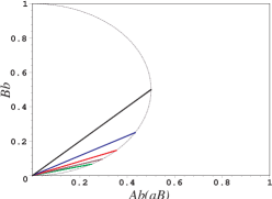
  Figure 8: Graphic of the straight line $C_{Ab(aB)}\,\mathrm{x}\,C_{Bb}$ with $\alpha=\pi/4,\pi/6,\pi/8,\pi/10\ \mathrm{and}\ \pi/12$ for the colors black, blue, red, brown and green, respectively. The slim violet curve is the semi circumference $(2C_{Bb}-1)^{2}+(2C_{Ab(aB)})^{2}=1$.

In order to interpret the expressions (25 – 29) and their respective figures (4 – 8), it becomes instructive to use the predictability,

$$\mathcal{P}_{0}=\Bigl{|}\mathrm{tr}\bigl{(}\sigma_{z}^{A}\rho_{0}\bigr{)}\Bigr{|}\ \ \ \ \ .$$ (30)

We use predictability because, unlike concurrence, it is measurable (the module of the mean value of an observable), local and it is related to the concurrence bergou . For $\rho_{0}=|\psi_{0}\rangle\langle\psi_{0}|$ we have $\mathcal{P}_{0}=|\cos(2\alpha)|$, and it is clear that $C_{0}^{2}+\mathcal{P}_{0}^{2}=1$. Observe that when $\mathcal{P}_{0}=0$ the excitation will be equally distributed between the partitions $Aa$ and $Bb$, it will not be localized and the initial entanglement will be maximum between $A$ and $B$. On the other hand, if $\mathcal{P}_{0}=1$ the atoms will not be initially entangled and the information if the excitation will be in partition $Aa$ or $Bb$ will not be available. However, we can assure that the excitation will be in the partition $Aa$ or in the partition $Bb$. When $0<\mathcal{P}_{0}<1$, all we know is that the excitation has a larger probability to be in one of the partitions.

The eccentricity of the ellipses (25) and (26) can be written as a function of the predictability

$$\epsilon=\sqrt{\dfrac{2\mathcal{P}_{0}}{1+\mathcal{P}_{0}}}\ \ \ \ .$$ (31)

We can determine also the distance $f$ of the focus to the center of each ellipse. For the ellipse (25) the distance of the focus $f^{(a)}$ to its center will be

$$f^{(a)}_{\lessgtr}=\sqrt{\dfrac{\mathcal{P}_{0}(1\mp\mathcal{P}_{0})}{2}},$$ (32)

where $f^{(a)}_{<}$ is the focus if $0<\alpha<\pi/4$ and $f^{(a)}_{>}$ is the focus if $\pi/4<\alpha<\pi/2$. The ellipse (26) will have the focus $f^{(b)}$ as being

$$f^{(b)}_{\gtrless}=\sqrt{\dfrac{\mathcal{P}_{0}(1\pm\mathcal{P}_{0})}{2}},$$ (33)

where $f^{(b)}_{>}$ is the focus if $0<\alpha<\pi/4$ and $f^{(b)}_{<}$ is the focus if $\pi/4<\alpha<\pi/2$, i. e. the opposite case of (32). This happens because the entanglement of the partition $Aa$ ($Bb$) is generated by the JCM evolution and not by the initial source of entanglement contained in $AB$. The entanglement generated by the JCM depends on the “quantity” of excitation that will be shared between the respective atom–field. Thus, when $0<\alpha<\pi/4$, the excitation, in the state represented by (3), will be more likely to be found in the partition $Aa$. Then, the entanglement generated by the JCM in the partition $Aa$ will be larger than $Bb$. This is represented in figure 5, where $C_{Aa}$ reaches larger values than $0.5$ if $0<\alpha<\pi/4$. In this case, the entanglement in the partition $Bb$ has values below 0.5, as we can observe in figure 4. The same analysis is valid in the opposite case, where $\pi/4<\alpha<\pi/2$. On the other hand, if $\alpha\in(0,\pi/2)$, the eccentricity of the ellipses (25) and (26) are identical, as shown in (31), but the focuses $f^{a}$ and $f^{b}$ do not have the same value and do not necessarily lie in the same axis, except for the case $\alpha=\pi/4$ when we have circumferences in both cases. For example, if $\alpha=\pi/6$ we have $f^{b}=\sqrt{3\,}f^{a}$, where $f^{a}$ ($f^{b}$) is over the horizontal (vertical) axis, respectively.

In section 3.1.3, equation (27) represents semi circumferences with radius $C_{0}/2$. When $\alpha=\pi/4$ ($C_{0}=1$) the limiting curve is obtained. More generally, we can say that a curve defined in its respective diagram $C_{ij}\,\mathrm{x}\,C_{kl}$ is always limited by the semi circumference $C_{ij}^{2}+C_{kl}^{2}=C_{0}^{2}$.

The sequential cases, represented by equations (28) and (29), are straight lines with angular coefficient dependent on the initial entanglement. As we did previously, we can write the angular coefficient as functions of the predictability. Equation(28) has angular coefficient $m^{(a)}$ given by

$$m^{(a)}_{\lessgtr}=\biggl{[}\dfrac{1-\mathcal{P}_{0}}{1+\mathcal{P}_{0}}\biggr{]}^{\pm 1/2}\ \ \ \ ,$$ (34)

where $m^{(a)}_{<}$ is the coefficient when $0<\alpha<\pi/4$ and $m^{(a)}_{>}$ is the coefficient if $\pi/4<\alpha<\pi/2$. Straight lines of equation (29) have angular coefficient

$$m^{(b)}_{\gtrless}=\biggl{[}\dfrac{1-\mathcal{P}_{0}}{1+\mathcal{P}_{0}}\biggr{]}^{\pm 1/2}\ \ \ \ ,$$ (35)

where, as in the previous case, $m^{(b)}_{<}$ is the coefficient if $0<\alpha<\pi/4$ and $m^{(b)}_{>}$ is the coefficient if $\pi/4<\alpha<\pi/2$. The opposite occurs for (34). This effect is also due to the entanglement given by the JCM as we already discussed previously in the ellipse equations (25) and (26).

3.2 For the initial state $|\phi_{0}\rangle$

Let us now consider the physical system whose initial state is given by equation (8). After a time interval $t$, the state of the system will be (9). In an analogous way as before we determine the concurrences of each pair of qubits. Those are

$${C}_{AB} = \max\bigl{[}0,C_{0}\cos^{2}(gt)-\gamma_{t}\bigr{]},$$ (36)

$${C}_{ab} = \max\bigl{[}0,C_{0}\sin^{2}(gt)-\gamma_{t}\bigr{]},$$ (37)

$${C}_{Aa} = \cos^{2}(\alpha)|\sin(2gt)|,$$ (38)

$${C}_{Ab} = \max\bigl{[}0,\dfrac{1}{2}C_{0}|\sin(2gt)|-\gamma_{t}\bigr{]},$$ (39)

$${C}_{aB} = \max\bigl{[}0,\dfrac{1}{2}C_{0}|\sin(2gt)|-\gamma_{t}\bigr{]},$$ (40)

$${C}_{Bb} = \cos^{2}(\alpha)|\sin(2gt)|\ \ \ \ \ ,$$ (41)

where $\gamma_{t}=\dfrac{1}{2}\cos^{2}(\alpha)\sin^{2}(2gt)$. Observe that if $0<\alpha<\pi/4$, we have entanglement sudden death morte or entanglement sudden birth nascimento .

In this case, we have some interesting situations due to the symmetry of the system. Notice that the partition $Aa$ and $Bb$ will have the same value of predictability. Thus, the dynamical entanglement supplied by the JCM to $Aa$ or $Bb$ is the same. Observe that ${C}_{Aa}={C}_{Bb}$. This would not be true if the coupling constant of each JCM was different. Due to that same symmetry we also have ${C}_{Ab}={C}_{Ba}$. Those relations define straight lines (like the case of equation (23)) in their respective diagrams. The other diagrams $C_{ij}\,\mathrm{x}\,C_{kl}$, however, are not so simple. That is because the initial state (8) contains the eigenstate $|00\rangle\otimes|00\rangle$ of the Hamiltonian (1), which does not contributes for the entanglement generated by the JCM, i. e. the time evolution of that eigenstate only adds a global phase to it (see eq. (11)). On the other hand, if the initial state is (2), both the states $|10\rangle\otimes|00\rangle$ and $|01\rangle\otimes|00\rangle$ contribute for the entanglement generated by the JCM in a form of senoidal functions of time in the amplitudes of the state (3) and that is why we obtain conics when we make parametric plots of concurrences.

The next case is in the diagram $C_{ab}\,\mathrm{x}\,C_{AB}$. Consider an instant of time when the concurrences ${C}_{AB}$ and ${C}_{ab}$ are different from zero at the same time. Then, we can write ${C}_{AB}=C_{0}\cos^{2}(gt)-\gamma_{t}$ and ${C}_{ab}=C_{0}\sin^{2}(gt)-\gamma_{t}$. Notice that using simple algebra we can write $[C_{0}-({C}_{AB}+{C}_{ab})]/\cos^{2}(\alpha)=\sin^{2}(2gt)$ and $({C}_{AB}-{C}_{ab})^{2}/C_{0}^{2}=\cos^{2}(2gt)$. Summing both we have

$$\dfrac{\bigl{(}{C}_{AB}-{C}_{ab}\bigr{)}^{2}}{C_{0}^{2}}+\dfrac{C_{0}-\bigl{(}{C}_{AB}+{C}_{ab}\bigr{)}}{\cos^{2}(\alpha)}=1\ \ \ \ .$$ (42)

This is a parabola with symmetry axis at $45^{\mathrm{o}}$ of the horizontal axis $({C}_{ab})$. On this axis the vertex $v$ is localized at point $v_{\lessgtr}=\{0,C_{0}-(1\pm\mathcal{P}_{0})/2\}$ and the focus $f$ at $f_{\lessgtr}=\{0,C_{0}\mp\mathcal{P}_{0}\}$, where the index $<$ ($>$) refers to $0<\alpha<\pi/4$ ($\pi/4<\alpha<\pi/2$), respectively. Because of the entanglement sudden death in the partitions $AB$ and $ab$ whenever $0<\alpha<\pi/4$, there will only be a segment of the parabola in the diagram ${C}_{ab}\,\mathrm{x}\,{C}_{AB}$ if the vertex $v$ admits positive values on the axis of the parabola. On the other hand, when the vertex is the origin or admits negative values, we will only have the straight line ${C}_{AB}=0$ or ${C}_{ab}=0$ (observe figure 9 for illustration).

Figure 9: Graphic of the parabola ${C}_{ab}\,\mathrm{x}\,{C}_{AB}$ with $\alpha=3\pi/10,\pi/4,\pi/5\ \mathrm{and}\ \pi/6$ for the colors blue, red, brown and green, respectively.

If $\alpha=\arctan(1/2)$ we have $v=\{0,0\}$ and when the entanglement in one of the partitions disappears the entanglement of another one resurges, as we see in figure 10.

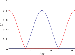
Figure 10: In red (blue) the graphic of ${C}_{AB}$ (${C}_{ab}$), respectively, for $\alpha=\arctan(1/2)$.

Following the same reasoning, it is clear that if $0<\alpha<\arctan(1/2)$ (or $\arctan(1/2)<\alpha<\pi/2$) the entanglement in $AB$ disappears before (or after) it appears in $ab$, respectively (this dynamics is depicted in figure 11).

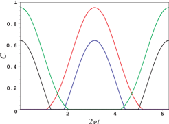
Figure 11: Graphic of ${C}_{AB}$ (${C}_{ab}$) in black (blue) when $\alpha=\pi/9<\arctan(1/2)$, respectively. Graphic of ${C}_{AB}$ (${C}_{ab}$) in green (red) when $\alpha=\pi/5>\arctan(1/2)$, respectively.

We keep seeking for more relations. Using the sum of equations (36) and (37), squaring them and adding to equations (38) or (41) squared, we get the following ellipse with expression

$$\dfrac{\bigl{(}{C}_{AB}-{C}_{ab}\bigr{)}^{2}}{C_{0}^{2}}+\dfrac{{C}^{2}_{Aa(Bb)}}{\cos^{4}\alpha}=1.$$ (43)

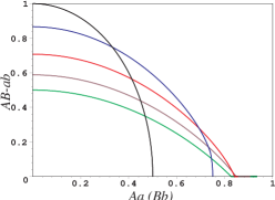
Figure 12: Graphic of the ellipse ${C}_{Aa(Bb)}\,\mathrm{x}\,\bigl{(}{C}_{AB}-{C}_{ab}\bigr{)}$ with $\alpha=\pi/4,\pi/6,\pi/8,\pi/10\ \mathrm{and}\ \pi/12$ for the colors black, blue, red, brown and green, respectively.

In figure 12, we show that we will always have a segment of the above ellipse, because the entanglement in $Aa$ does not suddenly disappear. If $0<\alpha<\arctan(1/2)$ the major semi–axis will be parallel to ${C}_{Aa(Bb)}$. When $\alpha=\arctan(1/2)$ we have a circumference and if $\arctan(1/2)<\alpha<\pi/2$, the major semi–axis will be parallel to ${C}_{AB}-{C}_{ab}$. The eccentricity of (43) is

$$\bar{\epsilon}=\left\{\begin{array}[]{rcl}\sqrt{\dfrac{5\mathcal{P}_{0}-3}{(1+\mathcal{P}_{0})}},&\mbox{if}&0<\alpha<\alpha_{0}\\ &&\\ \sqrt{\dfrac{3-5\mathcal{P}_{0}}{4(1-\mathcal{P}_{0})}},&\mbox{if}&\alpha_{0}<\alpha<\pi/4\\ &&\\ \sqrt{\dfrac{3+5\mathcal{P}_{0}}{4(1+\mathcal{P}_{0})}},&\mbox{if}&\pi/4<\alpha<\pi/2,\end{array}\right.$$ (49)

where $\alpha_{0}=\arctan(1/2)$. The focus is

$$\bar{f}=\left\{\begin{array}[]{rcl}\sqrt{(5\mathcal{P}_{0}-3)(1+\mathcal{P}_{0})}/2,&\mbox{if}&0<\alpha<\alpha_{0}\\ &&\\ \sqrt{(3-5\mathcal{P}_{0})(1+\mathcal{P}_{0})}/2,&\mbox{if}&\alpha_{0}<\alpha<\pi/4\\ &&\\ \sqrt{(3+5\mathcal{P}_{0})(1-\mathcal{P}_{0})}/2,&\mbox{if}&\pi/4<\alpha<\pi/2\ \ \ \ .\end{array}\right.$$ (55)

Observe that when $\alpha=\alpha_{0}$ we have $\mathcal{P}_{0}=3/5$, $\bar{f}=0$ and the ellipse becomes a semi circumference. Notice that if $0<\alpha<\alpha_{0}$, the entanglement of $AB$ disappears before the appearance of entanglement in $ab$. However, the entanglement of $Aa$ is given by the JCM and does not remain zero in any finite interval of time. As a result, there will be a time interval such that ${C}_{AB}-{C}_{ab}$ will be zero but the entanglement between $Aa$ will not. Thus, ${C}_{Aa}$ will admit values larger than ${C}_{AB}-{C}_{ab}$ and we have the major semi–axis parallel to ${C}_{Aa}$.

Consider now the expression used previously, $[C_{0}-({C}_{AB}+{C}_{ab})]/\cos^{2}(\alpha)=\sin^{2}(2gt)$. Using equation (38) or (41) we get another parabola whose equation reads

$$\bigl{(}{C}_{AB}+{C}_{ab}\bigr{)}=C_{0}-\dfrac{{C}_{Aa(Bb)}^{2}}{\cos^{2}\alpha}\ \ \ \ .$$ (56)

In figure 13, it becomes clear that the vertex $\tilde{v}$ and the focus $\tilde{f}$ are localized on the axis $\bigl{(}{C}_{AB}+{C}_{ab}\bigr{)}$ at points given by $\tilde{v}=\{0,\sqrt{1-(\mathcal{P}_{0})^{2}}\}$ and $\tilde{f}_{\lessgtr}=\{0,\sqrt{1-\mathcal{P}_{0}}-(1\pm\mathcal{P}_{0})\}$. As before, the sub–index is $<$ ($>$) if $0<\alpha<\pi/4$ ($\pi/4<\alpha<\pi/2$), respectively. We always have a segment of this parabola in the diagram $\bigl{(}{C}_{AB}+{C}_{ab}\bigr{)}\,\mathrm{x}\,{C}_{Aa(Bb)}$, because its vertex is limited between 0 and 1. We also know that $\bigl{(}{C}_{AB}+{C}_{ab}\bigr{)}$ will not be zero if $\alpha_{0}<\alpha<\pi/2$ and in this interval the parabola does not touch the axis ${C}_{Aa(Bb)}$.

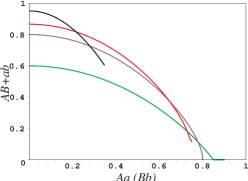
Figure 13: Graphic of the parabola ${C}_{Aa(Bb)}\,\mathrm{x}\,\bigl{(}{C}_{AB}+{C}_{ab}\bigr{)}$ with $\alpha=3\pi/10,\pi/6,\arctan(1/2)\ \mathrm{and}\ \arctan(1/3)$ for the colors black, red, brown and green, respectively.

And last but not least, we can write $|\sin(2gt)|={C}_{Aa(Bb)}\cos^{2}\alpha$ from equations (38) or (41) and substitute in (39) or (40). With some simplifications we have

$${C}_{Ab(aB)}+\dfrac{1}{2\cos^{2}\alpha}\biggl{(}{C}_{Aa(Bb)}-\dfrac{C_{0}}{2}\biggr{)}^{2}=\dfrac{C_{0}^{2}}{8\cos^{2}\alpha}.$$ (57)

That, like the previous case, is also a parabola with vertex $\breve{v}$ and focus $\breve{f}$ localized at points

$$\breve{v}_{\lessgtr} = \left\{\dfrac{\sqrt{1-\mathcal{P}_{0}^{2}}}{2},\dfrac{\bigl{(}1\mp\mathcal{P}_{0}\bigr{)}}{2}\right\},$$

$$\breve{f}_{\lessgtr} = \left\{\dfrac{\sqrt{1-\mathcal{P}_{0}^{2}}}{2},\dfrac{\mp\mathcal{P}_{0}}{2}\right\}.$$

The sub–index follows the previous notation. The parabola of equation (57) touches twice the axis ${C}_{Aa(Bb)}$ when $0<\alpha\leq\alpha_{0}$. This happens because if $0<\alpha<\alpha_{0}$, there is entanglement sudden death in the partition ${C}_{Ab(aB)}$. If $\alpha_{0}<\alpha<\pi/2$, on the other hand, there is not sudden death and the segment of the parabola only touches the axis ${C}_{Aa(Bb)}$ at the origin, as showed in figure 14.

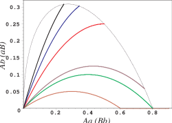
Figure 14: Graphic of the parabola ${C}_{Aa(Bb)}\,\mathrm{x}\,{C}_{Ab(aB)}$ with $\alpha=\pi/3,3\pi/10,\pi/4,\pi/6,\arctan(1/2)\ \mathrm{and}\ \arctan(1/3)$ for the colors black, red, brown, green and orange respectively.

4 The entanglement surface

In the previous section we explore the diagram $C_{ij}\,\mathrm{x}\,C_{kl}$ for two different initial states. Because of the unitary evolution of the physical model and the existence of an entanglement invariant distribuicao , it is relevant to analyze the three dimensional diagram $C_{ij}\,\mathrm{x}\,C_{ik}\,\mathrm{x}\,C_{il}$ for the $i$–th qubit. First we analyze such diagram for the atom $A$. For the initial state (2), the concurrences between the atom $A$ and any other qubit are given by equations (16), (18) and (19). If we make the parametric graphics of this concurrences we have curves, for a determined value of $\alpha$, in a diagram $C_{AB}\,\mathrm{x}\,C_{Aa}\,\mathrm{x}\,C_{Ab}$, as showed in figure 15.

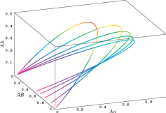
Figure 15: Graphic of the diagram $C_{AB}\,\mathrm{x}\,C_{Aa}\,\mathrm{x}\,C_{Ab}$ for the atom $A$ and initial state (2). From the superior curve to the inferior, we have, respectively, $\alpha=\pi/4,\pi/6,\pi/8,\pi/10\ \mathrm{and}\ \pi/12$.

Naturally, if we look at the projections of this curves in the planes $C_{AB}\,\mathrm{x}\,C_{Aa}$, $C_{AB}\,\mathrm{x}\,C_{Ab}$ and $C_{Aa}\,\mathrm{x}\,C_{Ab}$ we get the graphics drawn in figures 5, 6 and 7, respectively. If we draw all the possible curves (varying $\alpha$ from 0 to $\pi/2$) in the diagram $C_{AB}\,\mathrm{x}\,C_{Aa}\,\mathrm{x}\,C_{Ab}$ we have a surface in that space depicted in figure 16.

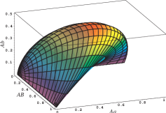
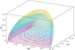
Figure 16: Entanglement surface for the atom $A$ in the diagram $C_{AB}\,\mathrm{x}\,C_{Aa}\,\mathrm{x}\,C_{Ab}$ for the initial state(2).

A point over that surface informs how much entanglement there is in each one of the partitions $AB$, $Aa$ and $Ab$. If now we consider the initial state (8) and draw the parametric graphics, for a few values of $\alpha$, in a diagram $C_{AB}\,\mathrm{x}\,C_{Aa}\,\mathrm{x}\,C_{Ab}$, we also have curves in that diagram, as depicted in figure 17.

Figure 17: Graphic of the diagram $C_{AB}\,\mathrm{x}\,C_{Aa}\,\mathrm{x}\,C_{Ab}$ for the initial state (8), with $\alpha=\pi/4,\pi/6,\pi/8,\pi/10\ \mathrm{and}\ \pi/12$.

As in the previous case we can draw all possible curves in the diagram $C_{AB}\,\mathrm{x}\,C_{Aa}\,\mathrm{x}\,C_{Ab}$ if we vary $\alpha$ from 0 to $\pi/2$ and we find an entanglement surface, see figure 18.

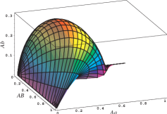
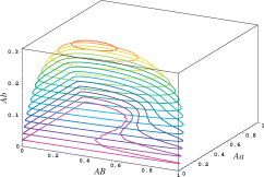
Figure 18: Entanglement surface of the atom $A$ in the diagram $C_{AB}\,\mathrm{x}\,C_{Aa}\,\mathrm{x}\,C_{Ab}$ for the initial state (8).

Points over this surface also gives how much entanglement there is in each of the subsystems $AB$, $Aa$ e $Ab$.

This same conclusions are also true for $B$, $a$ and $b$. So, in a general way, we can say that any trajectory in the diagrams $C_{ij}\,\mathrm{x}\,C_{ik}$, $C_{ij}\,\mathrm{x}\,C_{il}$ and $C_{ik}\,\mathrm{x}\,C_{il}$ belongs to the surface in $C_{ij}\,\mathrm{x}\,C_{ik}\,\mathrm{x}\,C_{il}$ and they are projections in its respective diagrams, where $i$, $j$, $k$ and $l$ are the 4 qubits ($A$, $B$, $a$ and $b$) of the system.

5 hyper-sphere shell of the entanglement dynamics

Next, we are going to use a result already obtained in distribuicao1 and geral2 . In these references, they observed that for the initial state (2) we have $C_{AB}^{2}+C_{Ab}^{2}+C_{aB}^{2}+C_{ab}^{2}=C_{0}^{2}$. Without loss of generality, we can sum in both sides the term $C_{Aa}^{2}+C_{Bb}^{2}$ and this yields $C_{AB}^{2}+C_{Ab}^{2}+C_{aB}^{2}+C_{ab}^{2}+C_{Aa}^{2}+C_{Bb}^{2}=C_{0}^{2}+(\cos^{4}\alpha+\sin^{4}\alpha)\sin^{2}(2gt)$. This last expression can be transformed in the inequality $C_{AB}^{2}+C_{Ab}^{2}+C_{aB}^{2}+C_{ab}^{2}+C_{Aa}^{2}+C_{Bb}^{2}\leq C_{0}^{2}+(\cos^{4}\alpha+\sin^{4}\alpha)$. Now, if we use simple trigonometric relations and the predictability, we can rewrite this equation as

$$C_{AB}^{2}+C_{Ab}^{2}+C_{aB}^{2}+C_{ab}^{2}+C_{Aa}^{2}+C_{Bb}^{2}\leq 1+\dfrac{C_{0}^{2}}{2},$$ (58)

which is a hyper-sphere with radius $\sqrt{(2+C_{0}^{2})/2\,}$ in a space where the axes are the concurrences between pairs of qubits. Besides, we can generalize the above inequality to

$$C_{0}^{2}\leq C_{AB}^{2}+C_{Ab}^{2}+C_{aB}^{2}+C_{ab}^{2}+C_{Aa}^{2}+C_{Bb}^{2}\leq 1+\dfrac{C_{0}^{2}}{2},$$ (59)

which defines a limited region (a hyper-sphere shell) inside the hypersphere defined by eq.(58). Thus, any curve in a diagram where the axes are concurrences between pairs of qubits and the initial state is (2) will lie either on the surface or in the interior of the hypersphere shell (59). So, we can speculate that, in the same way that curves in diagrams $C_{ij}\,\mathrm{x}\,C_{ik}$ are projections of curves of $C_{ij}\,\mathrm{x}\,C_{ik}\,\mathrm{x}\,C_{il}$, the surface defined in $C_{ij}\,\mathrm{x}\,C_{ik}\,\mathrm{x}\,C_{il}$ is a projection of the surface of a hypersphere that is in a space of greater dimension.

We can make the same analysis for the initial state (8). However, in that case distribuicao1 ; geral2 we have only the inequality $0\leq C_{AB}^{2}+C_{Ab}^{2}+C_{aB}^{2}+C_{ab}^{2}\leq C_{0}^{2}$ and, as done previously, we can sum both sides with the term $C_{Aa}^{2}+C_{Bb}^{2}=\bigl{[}1+\cos(2\alpha)\bigr{]}^{2}\sin^{2}(2gt)/2$. With a simple algebra we can express the result of this sum in the inequality $0\leq C_{AB}^{2}+C_{Ab}^{2}+C_{aB}^{2}+C_{ab}^{2}+C_{Aa}^{2}+C_{Bb}^{2}\leq C_{0}^{2}+[1+\cos(2\alpha)]^{2}/2$. We have the predictability $\mathcal{P}_{0}$ equals to $\cos(2\alpha)$ if $0<\alpha<\pi/4$ and $-\cos(2\alpha)$ if $\pi/4\leq\alpha\leq\pi/2$. Using this and $C_{0}^{2}+\mathcal{P}_{0}^{2}=1$ we can rewrite the inequality as

$$0\leq C_{AB}^{2}+C_{Ab}^{2}+C_{aB}^{2}+C_{ab}^{2}+C_{Aa}^{2}+C_{Bb}^{2}\leq 1+\frac{C_{0}^{2}}{2}\pm\mathcal{P}_{0},$$ (60)

where on the right hand side of the equation we will have $(1+C_{0}^{2}/2+\mathcal{P}_{0})$ when $0<\alpha<\pi/4$ and $(1+C_{0}^{2}/2-\mathcal{P}_{0})$ when $\pi/4\leq\alpha\leq\pi/2$. This inequality must be valid during the whole evolution and, in a space defined by the axes corresponding to the concurrences $C_{ij}$. We have the radius of the hyper-sphere given by

$$R_{\gtrless}=\sqrt{1+\frac{C_{0}^{2}}{2}\pm\mathcal{P}_{0}\,},$$ (61)

where we have $R_{>}$ ($R_{<}$) when $0<\alpha<\pi/4$ ($\pi/4\leq\alpha\leq\pi/2$), respectively. It is noteworthy that for $0<\alpha<\pi/4$ there is sudden death of entanglement in few partitions. On the other hand, for $\pi/4\leq\alpha\leq\pi/2$ there is not sudden death for any partition. Thus, we have $R_{>}$ when there is sudden death and $R_{<}$ otherwise. Note that for $0<\alpha<\arctan(1/2)$ there will be a time interval $\Delta\tau=[\arccos(\sqrt{\tan\alpha\,})-\arcsin(\sqrt{\tan\alpha\,})]/g$ where $C_{AB}=C_{ab}=C_{Ab}=C_{aB}=0$ (as observed in nascimento ). Since the hyper-sphere is defined by the concurrences between pairs of qubits, one would intuitively expect, in this conditions and during the time interval $\Delta\tau$, to obtain $R_{<}$ in place of $R_{>}$ since only $C_{Aa}$ and $C_{Bb}$ are different from zero. The increasing of the average radius is a consequence of the dynamical entanglement $C_{Aa}$ and $C_{Bb}$. When $0<\alpha<\pi/4$ the entanglement of the partitions $Aa$ and $Bb$ will attain maximum values between 1/2 and 1. Thus, the maximum value of $C_{Aa}^{2}+C_{Bb}^{2}$ will be between 1/2 and 2, contributing substantially to the inequality (60).

6 The effect of perturbation on conics

In this section, we consider the effect of decoherence in order to see how some conics of section 3 are affected. We consider the two cavities decaying freely, i. e. they both interact with a reservoir at zero temperature. This is a model closer to experimental reality.

The solution of the master equation for the initial state (2) gives us the density matrix for this case. We take the partial trace over the subsystems in order to obtain the following concurrences

$$C_{AB} = e^{-rz}|\sin 2\alpha|\left[\cos\left(\frac{z}{2}\right)+r\sin\left(\frac{z}{2}\right)\right]^{2},$$ (62)

$$C_{Aa} = e^{-rz}\sqrt{1+r^{2}}\cos^{2}\alpha|r(1-\cos z)+\sin z|,$$ (63)

$$C_{Bb} = e^{-rz}\sqrt{1+r^{2}}\sin^{2}\alpha|r(1-\cos z)+\sin z|,$$ (64)

$$C_{Ab} = \frac{1}{2}e^{-rz}\sqrt{1+r^{2}}|\sin 2\alpha||r(1-\cos z)+\sin z|,$$ (65)

$$C_{aB} = \frac{1}{2}e^{-rz}\sqrt{1+r^{2}}|\sin 2\alpha||r(1-\cos z)+\sin z|,$$ (66)

$$C_{ab} = e^{-rz}(1+r^{2})|\sin 2\alpha|\sin^{2}\left(\frac{z}{2}\right),$$ (67)

where $k$ is the decay constant, $\Omega=\sqrt{4g^{2}-k^{2}}$ is the Rabi frequency, $r=\frac{k}{\Omega}$ is the ratio between them and $z=\Omega t$. We recover eqs. (16)–(21) in the limit $k\rightarrow 0$.

Surprisingly enough, the curves (23), (24), (28) and (29) are not affected by this type of external coupling considered. On the other hand, if we consider one of the ellipses of subsection 3.1.1, we see that its size decreases with time. This result shows what we would expect, i.e. the decoherence destroys the entanglement between the atoms and the entanglement between an atom and its cavity (see figure 19). Of course, this effect also depends on how large $r$ is. Figure 19 and 19 shows examples where we see that the semi-axes go to zero in less time with the increasing of the external coupling.

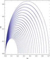
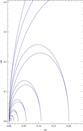
Figure 19: (a) Graphic of the semi–ellipse $C_{AB}\,\mathrm{x}\,C_{Aa}$ with $\alpha=\pi/8$, $r=0.01$ and $z\in[0,40\pi]$.(b) Graphic of the semi–ellipse $C_{AB}\,\mathrm{x}\,C_{Aa}$ with $\alpha=\pi/8$, $r=0.1$ and $z\in[0,20\pi]$

The straight line of equation (22) is also affected by the environment as we can see in figure 20. In this case, the intersection of the lines with the axes $C_{AB}$ and $C_{ab}$ shows that the initial available entanglement ($C_{0}$) is decreasing because the environment is monitoring the system.

Furthermore, we can notice by observing figures 19, 19 and 20 that the eccentricity of the ellipse and the angular coefficient do not change considerably with time. Therefore, it is possible to related those with predictability as done in section 3.

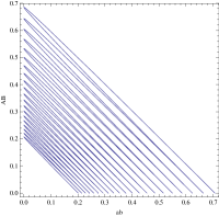
Figure 20: Graphic of the straight line $C_{AB}\,\mathrm{x}\,C_{ab}$ with $\alpha=\pi/8$, $r=0.01$ and $z\in[0,40\pi]$.

7 Conclusions

We presented a detailed study of the geometric character of the entanglement dynamics of two pairs of qubits evolving according to the DJCM. Although, this is an analytically solvable simple model, it exhibits a very rich dynamical structure which we explored here in order to give a geometric meaning to the entanglement dynamics. As it became clear, its very difficult to generalize our results to other more sophisticated models or initial conditions. However, we strongly believe that there is an intimate connection between the average radius of the hypersphere and the phenomenon of sudden death of entanglement. We hope to have provided for a tool which might aid experimentalists given that DJCM is within todays available technology.

References

- (1) A. Einstein, E. Podolsky, and N. Rosen, Phys. Review, 47, 777 (1935).
-
(2)
T. Yu, and J. Eberly, Phys. Rev. Let., 93,
140404 (2004).
M. Santos, P. Milman, L. Davidovich, and N. Zagury, Phys. Rev. A, 73, 040305 (2006).
T. Yu, Phys. Let. A, 361, 287 (2007).
Y.J. Zhang, Z.X. Man, and Y.J. Xia, J. Phys. B: At. Mol. Opt. Phys., 42, 095503 (2009). - (3) C. Lópes, G. Romero, F. Lastra, E. Solano, and J. Retamal, Phys. Rev. Let., 101, 080503 (2008).
- (4) J.S. Zhang, and J.B. Xu, Opt. Commun., 282, 3652 (2009).
- (5) S. Chan, M. Reid, and Ficek, J. Phys. B: At. Mol. Opt. Phys., 43, 215505(2010).
- (6) E. Jaynes, and F. Cummings, Proc. IEEE, 51, 89 (1963).
- (7) M. Tavis, and F. Cummings, Phys, Rev., 170, 379 (1968).
- (8) M. Yönaç, T. Yu, and J. Eberly, J. Phys. B: At. Mol. Phys., 39, S621 (2006).
- (9) H.T. Cui, K. Li, and X.X. Yi, Phys. Let. A, 365, 44 (2007).
- (10) Z.X. Man, Y.J. Xia, and N. An, J. Phys. B: At. Mol. Phys., 41, 085503 (2008).
- (11) D. McHugh, M. Ziman, and V. Buek, Phys. Rev. A, 74, 042303 (2006).
- (12) D. Cavalcanti, J. G. Oliveira Jr., J. G. Peixoto de Faria, M. Terra Cunha, and M. França Santos, Phys. Rev. A, 74, 042328 (2006).
- (13) I. Sainz, and G. Björk, Phys. Rev. A, 76, 042313 (2007).
- (14) M. Yönaç, T. Yu, and J. Heberly, J. Phys. B: At. Mol. Phys., 40, S45 (2007).
- (15) J.L. Guo, and H.S. Song, J. Phys. A: Math. Theor., 41, 085302 (2008).
- (16) S. Chan, M. Reid, and Z. Ficek, J. Phys. B: At. Mol. Phys., 42, 065507 (2009).
- (17) Z.X. Man, Y.J. Xia, and N.B. An, Eur. Phys. J. D, 53, 229 (2009).
- (18) W. K. Wootters, Phys. Rev. Lett., 80, 2245(1998).
- (19) M. Jakob, and J. Bergou, Opt. Commun., 179, 337 (2000).