A first-principles model of time-dependent variations in transmission through a fluctuating scattering environment

Abstract

Fading is the time-dependent variation in transmitted signal strength through a complex medium, due to interference or temporally evolving multipath scattering. In this paper we use random matrix theory (RMT) to establish a first-principles model for fading, including both universal and non-universal effects. This model provides a more general understanding of the most common statistical models (Rayleigh fading and Rice fading) and provides a detailed physical basis for their parameters. We also report experimental tests on two ray-chaotic microwave cavities. The results show that our RMT model agrees with the Rayleigh/Rice models in the high loss regime, but there are strong deviations in low-loss systems where the RMT approach describes the data well.

Considering wave propagation between a source and a receiver in a complex medium, fading is the time-dependent variation in the received signal amplitude as the scattering environment changes and evolvesSimon . Fading is a challenging problem in many situations where waves propagate through a complicated scattering environment. A common example is the nighttime variation of AM radio signal reception in the presence of ray bounce(s) off a time varying ionosphere. Another common observation of fading is experienced by radio listeners in automobiles moving among vehicles and buildings in an urban environment. Fading exists in closed or open scattering systems and in all types of wave propagation, and it is broadly studied in wireless communication, satellite-to-ground links, and time-dependent transport in mesoscopic conductors Simon ; Rayleigh_fading ; Foschini ; Delangre ; Rice_fading ; Lemoine ; buttiker .

The fading amplitude is defined as the ratio of the received signal to the transmitted signal. The traditional models Simon of fading work well in certain regimes of radiowave propagation applications, where different probability distribution functions are chosen depending upon the circumstances. However, these models are empirically designed for particular scattering environments and frequency bands, and different (apparently unrelated) fitting parameters are introduced in different models. For example, the Rayleigh fading model applies a one-parameter Rayleigh distribution for the fading amplitude in an environment where there is no line-of-sight (LOS) path between the transmitter and the receiver, such as mobile wireless systems in a metropolitan area Simon ; Rayleigh_fading ; Foschini ; Delangre . The Rice fading model, on the other hand, applies a two-parameter distribution for situations with a strong LOS path Simon ; Rice_fading ; Lemoine . The detailed physical origins of these models, and their parameters, are not clear.

The complexity of the wave propagation environment is advantageous from the perspective of wave chaos theory because it means that wave propagation is very sensitive to details, and a statistical description is most appropriate. For applying wave chaos approaches, the system should be in the semiclassical limit where the wavelength is much shorter than the typical size of the scattering system Stock . Researchers have applied random matrix theory (RMT) in wireless communication Tulino and analyzed the information capacity of fading channels Moustakas ; Morgenshtern ; Kumar , or the scattering matrix ($S$) and the impedance matrix ($Z$) of the scattering system Henry ; Brouwer ; Fyodorov . Here we directly apply the random matrix approach to the fading amplitude.

We derive a RMT-based fading model that includes the Rayleigh and Rice fading models in the high loss regime, but the RMT model also works well in the limit of low propagation loss. In addition, the RMT approach combined with a model of non-universal features reveals the precise physical meanings of the fitting parameters in the Rayleigh and Rice models.

Considering a $2\times 2$ scattering matrix $S$ which describes a linear relationship between the input and the output voltage waves on a network, the two ports can be assumed to correspond to the transmitter and the receiver. The fading amplitude is equivalent to the magnitude of the scattering matrix element $|S_{21}|$. We start with a RMT description of the $2\times 2$ universal scattering matrix $s_{rmt}$ in a wave chaotic system Brouwer . This description assumes total ergodicity and does not account for system specific information (such as the coupling of the ports and the short ray paths between the ports). For time-reversal invariant (TRI) wave propagation, statistics of $|s_{rmt,21}|$ can be generated from RMT, and the only parameter of the distribution $P(|s_{rmt,21}|;\gamma)$ is the dephasing rate $\gamma$ defined in Brouwer . Hemmady et al. Experimental_tests_our_work found the relationship between $\gamma$ and the loss parameter $\alpha$ of the corresponding closed system as $\gamma=4\pi\alpha$. The loss parameter $\alpha$ is the ratio of the closed-cavity mode resonance 3-dB bandwidth to the mean spacing between cavity modes, $\alpha\equiv f/(2Q\Delta f)$. Here $f$ is the frequency, $Q$ is the typical quality factor, and $\Delta f$ is the mean spacing of the adjacent eigenfrequencies. For an open fading system, we consider an equivalent closed system in which uniform absorption accounts for wave energy lost from the system, and we assume that we can define an equivalent loss parameter $\alpha$ for the open system Experimental_tests_our_work .

We can analytically derive the distribution of the fading amplitude $P(|s_{rmt,21}|;\alpha)$ for special cases of $\alpha$. For a lossless system ($\alpha=0$), the distribution of fading amplitude is a uniform distribution between 0 and 1. For high loss systems ($\alpha\gg 1$), we can prove that the distribution of fading amplitude goes to a Rayleigh distribution $P(x=|s_{rmt,21}|;\sigma)=\frac{x}{\sigma^{2}}\exp\left(\frac{-x^{2}}{2\sigma^{2}}\right)$ with the relationship

$$\alpha=\frac{1}{8\pi\sigma^{2}}.$$ (1)

This result reveals the physical meaning of the $\sigma$ parameter of the Rayleigh fading model, which assumes that the real and imaginary parts of the complex quantity $S_{21}$ are independent and identically distributed Gaussian variables with 0 mean and variance $\sigma^{2}$.

In Fig. 1 we illustrate $P(|s_{rmt,21}|;\alpha)$ for different loss parameter values from the RMT fading model. For higher loss cases, we also plot the corresponding Rayleigh distributions from Eq. (1) to show the convergence of the two models in the high loss limit. Note that distributions from the RMT model in the low loss region ($\alpha\leq 0.1$) deviate from a Rayleigh distribution.

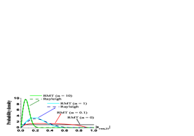
Figure 1: The probability density functions $P(|s_{rmt,21}|)$ generated from two theoretical models. Solid curves show the numerical results from the RMT model with different loss parameters ($\alpha=0,0.1,1,10$). For higher loss cases ($\alpha=1$ and $\alpha=10$), the corresponding Rayleigh distributions are shown as dashed curves.

To apply wave chaos theory to practical systems, in addition to the universal $s_{rmt,21}$, we also need to account for the non-chaotic features of the wave system. We employ the random coupling model (RCM) Hart ; Jenhao ; Experimental_tests_our_work , which combines universal fluctuating properties of a scattering system with the non-universal features arising from the port geometry and short-orbits between the ports, in the impedance matrix description. The impedance $(Z)$ matrix specifies the linear relationship between the port voltages and the port currents, and is related to the scattering matrix by $Z=Z_{0}(1+S)/(1-S)$, where $Z_{0}$ is a diagonal matrix with elements equal to the characteristic impedances of the transmission lines connected to the ports. Another method to deal with the coupling between the scattering channels and the system is the Poisson kernel that presents the non-chaotic features as an average $\bar{S}$ in the scattering matrix description Gopar ; Kuhl . The advantage of the RCM is that it can separate the chaotic (fluctuating) part and the non-chaotic (average) part in a simple additive format;

$$Z^{(the)}=iX_{avg}+R_{avg}^{1/2}(z_{rmt})R_{avg}^{1/2}.$$ (2)

$Z^{(the)}$ is the theoretical prediction of the raw measured impedance matrix $Z$, and $R_{avg}$ and $X_{avg}$ are the real and imaginary parts of the system-specific ensemble-averaged impedance matrix $Z_{avg}$. The matrix $Z_{avg}$ can be approximated by taking the average of the impedances of all realizations in a finite ensemble, $Z_{avg}=\bar{Z}$. The chaotic part is the universal impedance matrix $z_{rmt}=(1+s_{rmt})/(1-s_{rmt})$.

In the extended RCM Hart ; Jenhao , Hart et al. express the system-specific features in the ensemble wave-scattering system as

$$Z_{avg}^{(M)}=iX_{rad}+R_{rad}^{1/2}(z^{(M)}_{so})R_{rad}^{1/2},$$ (3)

where $R_{rad}$ and $X_{rad}$ are the real and imaginary parts of the radiation impedance matrix $Z_{rad}$, which is a diagonal matrix that quantifies the radiation and near-field characteristics of the ports. The other system-specific feature is short (major) trajectory orbits. We define an orbit as a ray trajectory that originates from one port, bounces on the boundary of the system or on scattering objects, and then reaches a port. Note that the line-of-sight signal between the two ports is the first (shortest) orbit, and that a short orbit is distinct from a periodic orbit in a closed system periodic_orbit . We can compute the short-orbits contribution matrix $z^{(M)}_{so}$ of the $M$ shortest orbits from the known geometry in each realization of the ensemble Hart ; Jenhao . The matrix elements $z^{(M)}_{so,a,b}=\sum_{m=1}^{M}P_{a,b}^{(m)}C_{a,b}^{(m)}\exp(iS_{a,b}^{(m)})$ is the sum of the short-orbit terms of the $M$ shortest orbits between port $a$ and port $b$. In each term we consider scattering on dispersing surfaces (in the geometry factor $C_{a,b}^{(m)}$), the survival probability ($P_{a,b}^{(m)}$) of the orbits due to the presence of mobile perturbers, and the propagation phase advance and loss (in the action $S_{a,b}^{(m)}$). The contribution of trajectory orbits decreases exponentially with the orbit length Hart ; Jenhao . In a lossy system $Z_{avg}^{(M)}\rightarrow Z_{avg}$ as $M$ increases Hart ; Jenhao , and only a limited number of short orbits are required to represent system-specific features that survive the ensemble average.

According to RMT, the universal complex parameter $s_{rmt,21}$ has zero mean, but the system-specific features of the sum of short orbits $z^{(M)}_{so}$ brings about a non-zero bias in the impedance matrix $Z_{avg}^{(M)}$ (or $Z_{avg}$). Therefore, the measured $S_{21}$ can have a non-zero mean, and this is similar in character to the Rice model. The Rice fading model use the distribution $P(x=|s_{rmt,21}|;\sigma,\nu)=\frac{x}{\sigma^{2}}\exp\left[\frac{-(x^{2}+\nu^{2})}{2\sigma^{2}}\right]I_{0}\left(\frac{x\nu}{\sigma^{2}}\right)$ which contains an additional parameter $\nu$ ($\nu\rightarrow 0$ recovers the Rayleigh distribution), and $I_{0}(\cdot)$ is the modified Bessel function of the first kind of order zero. The Rice model is an extension of the Rayleigh model in which the real and imaginary parts of $S_{21}$ are still independent and identical Gaussian variables with variance $\sigma^{2}$, but the means are generalized to a biased mean of magnitude $\nu$. The Rice fading model is used in environments where one signal path, typically the line-of-sight signal, is much stronger than the others Simon ; Rice_fading ; Lemoine , and the $\nu$ parameter is related to the strength of the strong signal. More generally, we find that the RMT fading model in the high loss limit yields an explicit expression for $\nu$ in terms of the short orbit impedance

$$\nu=|s_{so,21}^{(M)}|=\left|\frac{2z_{so,21}^{(M)}}{(1+z_{so,11}^{(M)})(1+z_{so,22}^{(M)})-(z_{so,21}^{(M)})^{2}}\right|.$$ (4)

This result generalizes the meaning of $\nu$ to include the influence of all major (short) paths. Note that when there is a single strong signal that dominates the sum of all paths, the $\nu$ parameter reverts to the original interpretation of Rice fading.

We have carried out experimental tests of the RMT fading model by measuring the complex $2\times 2$ scattering matrix $S$ in two quasi-two-dimensional ray-chaotic microwave cavities. Both of these cavities have two coupling ports, which we treat as a transmitter and a receiver. Microwaves are injected through each port antenna attached to a coaxial transmission line of characteristic impedance $Z_{0}=50\Omega$, and each antenna is inserted into the cavity through a small hole in the lid, similar to previous setups Experimental_tests_our_work ; Jenhao ; Dietz . The waves introduced are quasi-two-dimensional for frequencies below the cutoff frequency for higher order modes ($\sim 19$ GHz) due to the thin height of the cavities (8 mm in the $z$-direction).

Classical ray-chaos arises from the shape of the cavity walls. One cavity is a symmetry-reduced “bow-tie billiard” made up of two straight walls and two circular dispersing walls Experimental_tests_our_work ; Jenhao shown in Fig. 2(c), and the other cavity is a “cut-circle billiard” Dietz shown in Fig. 2(d). The scales of the billiards compared to the wavelengths of the microwave signals ($1.7-5.0$ cm) put these systems into the semiclassical limit. To create an ensemble for statistical analysis, we add two cylindrical metal perturbers to the interior of the $1/4$ bow-tie cavity and systematically move the perturbers to create 100 different realizations. For the cut-circle cavity, the perturber is a Teflon wedge that can be rotated inside the cavity. We rotate the wedge by 5 degrees each time and create 72 different realizations. The perturbers can be considered as scattering objects in the propagation medium, so changing the positions creates the equivalent of time-dependent scattering variations that give rise to fading. The $1/4$ bow-tie cavity is made of copper, and measurements of the transmission spectrum at room temperature suggest the loss parameter goes from $\alpha=0.4$ to $1.0$, varying with the frequency range Jenhao . The superconducting cut-circle cavity is made of copper with Pb-plated walls and cooled by a pulsed tube refrigerator to a temperature of 5.5 K, below the transition temperature of Pb Richter ; Dietz . Measurements of the transmission spectrum suggest $\alpha<10^{-1}$.

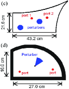
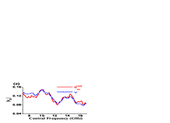
Figure 2: Probability density functions $P(|s_{rmt,21}|)$ from the experimental data (red circles) in (a) the $1/4$ bow-tie cavity and in (b) the cut-circle cavity, comparing with the RMT model (black solid) and the best-matched Rayleigh distribution (blue dashed). (c) The $1/4$ bow-tie cavity with the two ports as red dots and the two perturbers as blue circles. (d) The cut-circle cavity with the two ports as red dots and the perturber as a blue wedge. (e) Magnitude of $|s_{so,21}^{(M)}|$ averaged over a 2-GHz frequency band versus the central frequency in the $1/4$ bow-tie cavity, and the $\nu$ parameter of the best-matched Rice distribution.

The experimental data show good agreement with our RMT fading model. We first use $Z^{(the)}$ in Eq. (2) to represent the measured impedance matrix $Z$ and solve for $z_{rmt}$ (and therefore $s_{rmt}$). In this process we remove the system-specific features including all short orbits, so the situation is equivalent to the Rayleigh fading environment where no direct paths exist. By choosing data over all realizations in a frequency range, we can construct the distribution of $|s_{rmt,21}|$ and compare with the prediction of RMT. In Fig. 2 (a) and (b) we plot the distributions of the fading amplitude from the RMT model (black solid), the experimental data (red circles), and a best-matched Rayleigh distribution (blue dashed). In Fig. 2(a) the room-temperature case, the best-matched RMT model gives a value of the loss parameter $\alpha=0.5$ for the experimental data, which corresponds to $\sigma\simeq(8\pi\alpha)^{-0.5}=0.282.$ The best-matched Rayleigh distribution yields $\sigma=0.226.$ The difference in $\sigma$ values is due to the fact that the loss parameter is not very large in this case. Nevertheless, both models agree with the experimental data well in this loss regime. In Fig. 2(b) the superconducting cavity case, the agreement between the experimental data and the RMT model is much better than the Rayleigh distribution. In fact, in the very-low-loss region ($\alpha<<1$), the long exponential tail of a Rayleigh distribution can never match the RMT theoretical distribution that is limited to $0\leq|s_{rmt,21}|\leq 1$.

In the room-temperature case, since the loss parameter is high enough, we can compare the relationship between the RMT model and the Rice fading model [Eq. (4)]. In Fig. 2(e), we compute $z_{so}^{(M)}$ to include short orbits with length up to 200 cm ($M=1088$) in the $1/4$ bow-tie cavity, apply Eq. (4), perform a sliding average over a 2-GHz frequency band, and plot the magnitude $|s_{so,21}^{(M)}|$ as the red curve. For the $\nu$ parameter of the Rice model, we first remove the coupling features from the measured impedance ($Z$) matrix as $z=R_{rad}^{-1/2}(Z-iX_{rad})R_{rad}^{-1/2}$ and convert the impedance matrix $z$ to $s$. Then we compare the distribution of $|s_{21}|$ over a 2-GHz frequency band and 100 realizations with the best-matched Rice distribution. Since the $\sigma$ parameter has been determined by the best-matched Rayleigh distribution as described above for the fully universal data [Fig. 2(a)], we can use $\nu$ as the only fitting parameter. In Fig. 2(e) we plot the $\nu$ parameter for the best-matched Rice distributions (blue squares) along with the system-specific average magnitudes of $s_{21}$ versus the central frequency of a 2-GHz frequency band. The value of the Rice $\nu$ parameter and the system-specific feature described by our model agree well.

One more advantage of applying the RCM is that we can extend the relations Eq. (1) and (4) from the normalized data to the raw measured data in the high loss cases. In high loss cases, the magnitude of the elements of $s_{rmt}$ are much less than one, so we take the approximation to the lowest order Gradoni . For the generalized $\tilde{\nu}$ parameter, we only need to replace the $z_{so}^{(M)}$ terms by $Z_{avg}$ or $Z_{avg}^{(M)}$ in Eq. (4). The generalized $\tilde{\sigma}$ parameter is a function of $\alpha$ and all elements of the matrix $Z_{avg}$. If the transmission between the ports is much less than the coupling reflection at the ports (i.e. $|Z_{avg,21}|\ll|Z_{avg,11}|,\ |Z_{avg,22}|$), the modified Rayleigh $\tilde{\sigma}$ parameter can be simplified to

$$\tilde{\sigma}\simeq\sigma\frac{4\sqrt{Z_{0,11}R_{avg,11}Z_{0,22}R_{avg,22}}}{|Z_{0,11}+Z_{avg,11}||Z_{0,22}+Z_{avg,22}|}.$$ (5)

In conclusion, we have provided a first-principles derivation of a RMT fading model that reduces to the traditional Rayleigh and Rice fading models in high-loss scattering environments, and hence we can explain the physical meanings of the $\sigma$ parameter of the Rayleigh distribution and the $\nu$ parameter of the Rice distribution. Moreover, in low-loss environments, the RMT model can better predict the distribution of the fading amplitude $|S_{21}|$. Because wave propagation in a complicated environment is a common issue in many fields Simon ; Rayleigh_fading ; Foschini ; Delangre ; Rice_fading ; buttiker , the fading model can be applied to wireless communication, global positioning systems, and mesoscopic physics.

We thank the group of A. Richter (Uni. Darmstadt) for graciously loaning the cut-circle billiard. This work is funded by the ONR/Maryland AppEl Center Task A2 (contract No. N000140911190), the AFOSR under grant FA95500710049, and Center for Nanophysics and Advanced Materials (CNAM).

References

- (1) M. Simon and M.-S. Alouini, Digital Communication over Fading Channels, 2nd ed., (John Wiley & Sons, Inc., 2005).
- (2) G. L. Stüber, Principles of Mobile Communications (Kluwer Academic Publishers, Norwell, MA, USA, 1996).
- (3) G. J. Foschini, Bell Labs Technical J., 1, 41 (1996).
- (4) O. Delangre et al., C. R. Physique 11, 30 (2010).
- (5) M. Nakagami, in W. C. Hoffman, Statistical Methods in Radio Wave Propagation (Pergamon Press 1960).
- (6) C. Lemoine, E. Amador, and P. Besnier, Electronics Lett. 47, 20 (2011).
- (7) M. Büttiker, J. Low Temp. Phys. 118, 519 (2000).
- (8) H. J. Stöckmann, Quantum Chaos (Cambridge University Press, New York, 1999).
- (9) A. M. Tulino and S. Verdú, Random Matrix Theory and Wireless Communications Foundations and Trends in Commun. and Inf. Theory, 1, 1 (2004).
- (10) A. L. Moustakas et al., Science 287, 287 (2000); S. H. Simon et al., Physics Today 54, 38 (2001); A. L. Moustakas and S. H. Simon, J. Phys. A: Math. Gen. 38, 10859 (2005).
- (11) V. I. Morgenshtern and H. Bölcskei, IEEE Trans. on Information Theory, 53, 10, (2007).
- (12) S. Kumar and A. Pandey, IEEE Trans. on Information Theory, 56, 5, (2010).
- (13) X. Zheng, T. M. Antonsen Jr., and E. Ott, Electromagnetics 26, 3 (2006); Electromagnetics 26, 37 (2006); X. Zheng et al., Phys. Rev. E 73 , 046208 (2006).
- (14) P. W. Brouwer and C. W. J. Beenakker, Phys. Rev. B 55, 4695 (1997).
- (15) I. Rozhkov, Y. V. Fyodorov, and R. L. Weaver, Phys. Rev. E 68, 016204 (2003); Phys. Rev. E 69, 036206 (2004); Y. V. Fyodorov, D. V. Savin, and H.-J. Sommers, J. Phys. A: Math. Gen. 38, 10731 (2005).
- (16) S. Hemmady et al., Phys. Rev. Lett. 94, 014102 (2005); Phys. Rev. E 71, 056215 (2005); Phys. Rev. E 74, 036213 (2006); Phys. Rev. B 74, 195326 (2006).
- (17) J. A. Hart, T. M. Antonsen, and E. Ott, Phys. Rev. E 80, 041109 (2009).
- (18) J.-H. Yeh et al., Phys. Rev. E 81, 025201(R) (2010); Phys. Rev. E 82, 041114 (2010).
- (19) U. Kuhl et al., Phys. Rev. Lett. 94, 144101 (2005).
- (20) V. A. Gopar, M. Martínez-Mares, and R. A. Méndez-Sánchez, J. Phys. A: Math. Theor. 41, 015103 (2008).
- (21) D. Wintgen and H. Friedrich, Phys. Rev. A 36, 131 (1987); J. Stein and H.-J. Stöckmann, Phys. Rev. Lett. 68, 2867 (1992); M. Sieber and K. Richter, Phys. Scr. T 90, 128 (2001).
- (22) B. Dietz et al., Phys. Rev. E 73, 035201(R) (2006); Phys. Rev. E 78, 055204 (2008).
- (23) A. Richter, Phys. Scr. T90, 212 (2001).
- (24) G. Gradoni, J.-H. Yeh, T. M. Antonsen, S. M. Anlage, E. Ott, Proc. of the 2011 IEEE EMC Symposium.