Spectroscopy of Luminous Compact Blue Galaxies
in Distant Clusters I. Spectroscopic Data

Abstract

We used the DEIMOS spectrograph on the Keck II Telescope to obtain spectra of galaxies in the fields of five distant, rich galaxy clusters over the redshift range $0.5<z<0.9$ in a search for luminous, compact, blue galaxies (LCBGs). Unlike traditional studies of galaxy clusters, we preferentially targeted blue cluster members identified via multi-band photometric pre-selection based on imaging data from the WIYN telescope. Of the 1288 sources that we targeted, we determined secure spectroscopic redshifts for 848 sources, yielding a total success rate of $66\%$. Our redshift measurements are in good agreement with those previously reported in the literature, except for 11 targets which we believe were previously in error. Within our sample, we confirm the presence of 53 LCBGs in the five galaxy clusters. The clusters all stand out as distinct peaks in the redshift distribution of LCBGs with the average number density of LCBGs ranging from $1.65\pm 0.25~{}\mbox{Mpc}^{-3}$ at $z=0.55$ to $3.13\pm 0.65~{}\mbox{Mpc}^{-3}$ at $z=0.8$. The number density of LCBGs in clustes exceeds the field desnity by a factor of $749\pm 116$ at $z=0.55$; at $z=0.8$, the corresponding ratio is $E=416\pm 95$. At $z=0.55$, this enhancement is well above that seen for blue galaxies or the overall cluster population, indicating that LCBGs are preferentially triggered in high-density environments at intermediate redshifts.

1 Introduction

The first provocative evidence of galaxy evolution in the Universe was the increasing fraction of blue galaxies in clusters reported in the now-classic papers by Butcher & Oemler (1978, 1984). In these early papers, based purely on photometry, the large scatter in the blue fraction from cluster to cluster – along with some counter examples of very red clusters at what was then considered “high” redshift (e.g. Cl 0016+16 by Koo 1981) – made it unclear just how rapidly and uniformly cluster populations were evolving. Despite the passage of three decades since the first publication of these papers, we still lack a definitive picture of how star-forming populations in galaxy clusters evolve. The situation among cluster galaxies stands in stark contrast to the substantial evolution observed in the field galaxy population, in which abundant redshift surveys have now revealed a rapid rise in the star formation rate to $z=1$ (Cooper et al. 2008). A major impediment to improving the understanding of cluster evolution has been a lack of studies probing the star-forming populations in clusters, especially at intermediate redshifts ($0.3<z<1.0$).

The first confirmation of blue, cluster galaxies was by Dressler & Gunn (1982); they used spectroscopic observations to confirm the cluster membership of the objects and explore their properties. Further spectroscopic observations of clusters indicated a group of transitional objects (e.g., “E+A” galaxies, Dressler & Gunn 1983) that could provide a link between actively star-forming objects (in what is today referred to as the “blue cloud”) and passive galaxies lying on the “red sequence” (Couch & Sharples 1987, Wirth et al. 1994, Barger et al. 1996, Tran et al. 2003).

The stark difference between the cluster and the field populations – as described by the morphology-density relationship (Dressler et al. 1980) or the star formation-density relationship (Gomez et al. 2003) – prompted investigators to invoke numerous mechanisms that would lead to an environmental dependence in galaxy formation and evolution. In a hierarchical formation model, galaxies falling into the cluster environment are transformed into a quiescent population through a variety of mechanisms that extinguish star formation via gas starvation, stripping, and/or pre-processing (see the review by Boselli and Gavazzi 2006). Evidence for these different processes has been observed at both low and high redshift, and these transformations apparently start well outside the cluster virial radius (Porter & Raychaudhury 2005, Poggianti et al. 2009).

One of the first attempts to produce a comprehensive inventory of star-forming population of an intermediate redshift cluster was a narrow-band imaging survey by Martin, Lotz, and Ferguson (2000) of Abell 851 at $z=0.45$ targeting [O II] $\lambda 3727$ emission. They reported an overabundance of star-forming galaxies in the clusters as compared to the field at similar redshift, but this result was not confirmed by their subsequent observations of the lower mass cluster MS 1512.4+3647 at $z=0.372$ (Lotz, Martin, and Ferguson 2003). However, Abell 851 is a far more massive cluster with significant evidence of substructure, so differences between the star-forming populations may be related to the different properties and evolutionary states of the clusters. Finn et al. (2004) expanded on these measurements with H$\alpha$ narrow-band observations of intermediate-redshift clusters, finding an increase in the total star formation rate with increasing redshift among the cluster population (Finn et al. 2008) that matches the increase which is found in the global star formation rate (Madau et al. 1997, Cooper et al. 2008).

The presence of obscured star-forming galaxies further complicates the picture of star formation in clusters. Radio continuum observations provided the first evidence for the presence of these sources (Miller & Owen 2002), and a series of studies at far-infrared wavelengths has found a large number of heavily-obscured star-forming galaxies (Saintonge, Tran, and Holden 2008; Gallazzi et al. 2009; Haines et al. 2009). In follow-up spectroscopy to their narrow-band observations of A851, Sato & Martin (2006a, 2006b) identified a population of heavily-reddened, star-forming galaxies and bursting dwarf populations. It remains a challenge to explain the properties of these objects and how they pertain to the evolution of cluster galaxies (Smith et al. 2010), and in particular, the connection, if any, to the star-forming population that is not heavily obscured.

To illuminate the interplay between environment and evolution, a large number of recent spectroscopic surveys has targeted clusters at intermediate redshift (Postman et al.  2001, Tran et al.  2003, Halliday et al.  2004, Sato & Martin 2006a, Moran et al.  2007, Tanaka et al. 2007). Only with this added kinematic information can we determine whether we are seeing galaxies that are falling into the cluster for the first time, a backsplash population of objects (Pimbblet 2011), or objects forming in-situ in the cluster such as tidal dwarfs (Duc & Bournaud 2008). By extending the kinematic coverage to a comprehensive sample of the cluster star-forming galaxies, we can then hope to establish a clear connection between these star-forming galaxies at intermediate redshift and the populations seen in clusters today.

In this paper, we specifically focus on Luminous Compact Blue Galaxies (LCBGs), an extreme star-forming class of galaxies initially identified in the field at intermediate redshifts (Koo et al. 1994). Their sharp drop in number density with decreasing redshift mimics the decline in the global star formation rate (Guzman et al. 1997, Werk et al. 2004), and the population appears to be a heterogeneous mix of bursting dwarfs and star-forming bulges (Guzman et al. 1996, Garland et al. 2004, Noeske et al. 2006, Rawat et al. 2007, Tollerud et al. 2010). Due to this observed mix, LCBGs are proposed either to evolve into spheroidal systems (Koo et al. 1994, Guzman et al. 1996) or to be an intermediate phase in the evolution of bulge-dominated spiral galaxies (Phillips et al. 1997, Hammer et al. 2001).

Follow-up observations of a small sample of blue galaxies in Cl 0024+1654 at $z=0.39$ by Koo et al. (1997) provided the first confirmation of LCBGs in galaxy clusters. Crawford et al. (2006) found an enhancement in these types of galaxies among intermediate redshift clusters based purely on photometric information, thus suggesting an increase in both their number density and fraction of galaxies with galaxy density. Further spectroscopic confirmation of cluster LCBGs was reported by Moran et al. (2007) in MS 0451-03 at $z=0.54$.

In this paper, we introduce our survey and present optical spectroscopic measurements obtained from two observing runs with the DEIMOS spectrograph on the Keck II Telescope. In §2, we describe the WIYN Long Term Variability survey from which our sample was selected. In §3, the spectroscopic observations from sample selection to data reduction are presented. In §4, we provide the catalog of targeted objects. We discuss the quality of our redshift measurements in §5. Finally, we briefly examine the evolution of cluster LCBGs with environment and redshift in §6.

Throughout this work, we adopt $H_{0}=70$ km s^-1 Mpc^-1, $\Omega_{M}=0.3$, and $\Omega_{\Lambda}=0.7$; all magnitudes are in the Vega system.

2 The WLTV Survey

The WIYN Long Term Variability (WLTV) survey is a photometric census of ten massive galaxy clusters over the redshift range $0.3<z<0.9$ undertaken with the WIYN 3.5 m telescope. The observational aim of the survey was to acquire deep, multi-epoch photometry from the near-UV to the near-IR in very rich clusters at intermediate redshifts. The observations were completed over a 6-year period and sample the time domain on scales of one month up to the survey duration. Our extragalactic scientific goals include detailed star formation and stellar population studies of individual cluster galaxies; cluster populations as well as galaxies in the foreground, background, and cluster outskirts; and a search for transients (supernovae) and AGN variability in galaxies within the field of rich clusters. The photometric band-passes and depth chosen to achieve these goals are described in §2.2.

2.1 Cluster Sample

As detailed in Crawford et al. (2009), we established the following three key criteria to select clusters for the survey:

1. general recognition in the literature that the cluster represents a significant, high-redshift overdensity in the galaxy distribution;

2. availability of Hubble Space Telescope (HST) imaging data of the field to permit accurate measurements of galaxy size and morphology;

3. existence of significant followup spectroscopy establishing the overdensity as a bona-fide cluster rather than a chance superposition.

Since the start of the WLTV observing campaign in 1999, many of these clusters have been observed by others across a wide range of wavelengths. From this sample, we have selected the five highest-redshift, most massive clusters for further investigation. Details of the five selected clusters are provided in Table 1. In this table, we provide the cluster name, the survey identifier for each cluster, redshift, cluster velocity dispersion, $M_{200}$ and $R_{200}$ radius for each cluster. The cluster velocity dispersion is calculated based on all available spectroscopic data following a method similar to Fadda et al. (1996), and the full details of the calculations will be given in future work. A description of each of the major clusters is provided below:

• MS 0451-03 is a rich, well-studied cluster at $z=0.53$ initially discovered by Stocke et al. (1991) in the Einstein Medium Sensitivity Survey (EMSS) and spectroscopically confirmed by Gioia & Luppino (1994). MS 0451-03 is X-ray luminous (Donahue et al. 2003), with over 300 spectroscopically-confirmed members (Ellingson et al. 1998, Moran et al. 2007). Cluster mass estimates are available from the velocity dispersion of cluster galaxies (Carlberg et al. 1996), X-ray luminosity (Donahue et al. 2003), and weak-lensing analysis (Clowe et al. 2000).

• Cl 0016+16 is one of the first clusters found to defy the reported increase in the fraction of blue cluster galaxies at intermediate redshift (Koo 1981). Specifically, the core of this elongated cluster has few blue galaxies. Cl 0016+16 is a rich cluster at $z=0.55$ with over 200 spectroscopically confirmed members (Wirth et al. 1994, Ellingson et al. 1998, Dressler et al. 1999, Tanaka et al. 2007). It is the major component of a supercluster complex (Connolly et al. 1996, Tanaka et al. 2005, 2007). X-ray observations of the cluster reveal a luminous system with multiple substructures (Worrall & Birkinshaw 2003), but yield mass estimates comparable to other measurements based on galaxy velocity dispersion and weak lensing (Smail et al. 1997, Carlberg et al. 1997, and Clowe et al. 2000).

• Cl J1324+3011 was originally discovered by Gunn, Hoessel, & Oke (1986) and spectroscopically confirmed as a cluster at $z=0.75$ by Oke, Postman & Lubin (1998). XMM-Newton observations of the cluster indicate it is under-luminous for its velocity dispersion as compared to local galaxy clusters (Lubin, Mulchaey, & Postman 2004).

• MS 1054-03 is a massive cluster at $z=0.83$ that has been extensively studied both through HST imaging and spectroscopy (van Dokkum et al. 1999, Tran et al. 1999, Goto et al. 2005, Tran et al. 2005). Initially discovered as one of the highest-redshift sources in the EMSS (Stocke et al. 1991), MS 1054-03 has been shown to be a massive cluster at high redshift on the basis of spectroscopic velocity dispersion measurements (Tran et al. 1999), X-ray luminosity (Donahue et al. 1998, Neumann & Arnaud 2000, Jeltema et al 2001, Gioia et al. 2004), and weak-lensing mass estimates (Luppino & Kaiser 1997, Clowe et al. 2000, Jee et al. 2005).

• Cl J1604+4304 is the highest-redshift cluster in our sample at $z=0.90$ (Oke, Postman, Lubin 1998). It forms part of a supercluster complex (Gal & Lubin 2004) and exhibits an overdensity of AGN (Kocevski et al. 2009). The X-ray luminosity of the cluster is lower than predicted from the measured velocity dispersion (Lubin et al. 2004). The uncertainty in the mass from a weak-lensing estimate does not allow strong constraints on the cluster mass, but does confirm the presence of a massive structure at high redshift (Margoniner et al. 2005).

All of the clusters in our sample are massive, and due to their predicted growth, they are likely to all have similar mass to each other if observed today. Following the models of Wechsler et al. (2002) for the growth of dark matter structures, we would predict these structures to have a velocity dispersion $\sigma\sim 1500$ km s^-1 and masses of $6\times 10^{15}M_{\odot}$ at the present epoch.

2.2 Imaging Survey

The core of the time-domain WLTV imaging survey consisted of $UBRI$ imaging with the Mini-Mosaic camera ($10\arcmin$ field of view with $0\farcs 14~{}\mbox{px}^{-1}$) on the WIYN 3.5 m telescope over six years from October 1999 until June 2005. For the purposes of deriving photometric redshifts and rest-frame $B$-band properties of the highest-redshift cluster galaxies, the data were supplemented with deep $z$-band imaging that we obtained at WIYN with the same instrument. The typical limiting magnitude of each field is $R\sim 25.5$, with similar depth in the other passbands. Full details of the observations, data reduction, and analysis appear in Crawford et al. (2009).

For the highest-redshift clusters among the sample, we designed a set of custom narrow-band filters to observe the [O II] $\lambda 3727$  spectral feature in star-forming galaxies at the redshift of each cluster. The width of each narrow-band filter was set by the velocity dispersion of the cluster and is typically $\sim 100$ Å. Observations were obtained through the narrow-band filters for a minimum of 3.5 h using the same instrumentation and telescope as for the broad-band imaging program. We also observed each cluster with an off-band narrow-band filter that is close to the on-band filter, but sufficiently different in central wavelength to avoid contamination from cluster sources. Measurements of the strength of the [O II] $\lambda 3727$  feature were derived from fits to the full spectral energy distribution and are used in our selection of spectroscopic targets. Full details of the narrow-band filters and data reduction are presented in Crawford (2006).

3 Spectroscopic Observations

3.1 Sample Selection & Masks

Since the aim of our present investigation is to identify star-forming cluster galaxies, we deviated from the customary strategy for observing high-redshift clusters by preferentially selecting blue (rather than red) cluster objects for spectroscopy. These targets were selected on the basis of photometric measurements derived from the WLTV narrow-band survey data. Potential emission-line galaxies were identified via a flux excess in the on-band filter combined with the estimated photometric redshift. Due to improvements in the technique of measuring the flux excess, our selection criteria differed between the two Keck observing runs as described below.

For the November 2005 run which included Cl 0016+16 and MS0451-03, we assigned top priority to objects classified as LCBGs. As further discussed in §4.2, we adopted the definition from Crawford et al. (2006) with LCBGs defined as galaxies with $(B-V)_{o}<0.5$, $\mu_{B}<21$ mag arcsec^-2, and $M_{B}<-18.5$. Next highest priority was given to other cluster star-forming galaxies; i.e., objects showing blue colors and an excess in the narrow-band filter sampling [O II] $\lambda 3727$  at the cluster redshift as compared to the continuum filter. Specifically, these blue objects were defined as having $B-I<2.5$ mag and $C-E>0.2$ mag where $E$ is the measured flux within the [O II] $\lambda 3727$  filter for each cluster and $C$ is the flux within the corresponding blueward continuum filter. The apparent color of $B-I=2.5$ would correspond to having a rest-frame color of $(B-V)_{o}\sim 0.5$ at $z=0.55$. For each class of objects, higher priority for selection was granted to sources with a spectroscopic or photometric redshift within $|\Delta z|\leq 0.1$ of the nominal cluster redshift. Finally, brighter galaxies were given higher selection priority to maximize the resulting number of usable spectra. We applied an apparent magnitude cut at $R<24.0$ and rejected bright stars (defined as having $R<22.5$ and a half-light radius of $r_{0.5}<0\farcs 5$). Because each DEIMOS mask covers an area much larger than the WIYN field of view, we used $R$-band pre-imaging obtained with DEIMOS to select additional targets for spectroscopy in areas outside the WLTV survey field. These objects were selected purely based on their $R$-band magnitude with preference given to brighter objects.

For the April 2007 run which included MS 1054-03, Cl J1324+3011, and Cl 1604+4304; we modified the selection criteria to include information from the improved determination of the narrow-band flux. We preferentially selected cluster emission-line objects, identified as having a high probability of cluster membership based on on-band flux, color, and photometric redshift. The on-band flux was determined by fitting the full observed Spectral Energy Distribution (SED) with model SEDs and then subtracting off the continuum value at the on-band filter. We assigned the next highest priority to potential high-redshift QSOs and Ly $\alpha$ galaxies, respectively, both of which were selected based on their colors using the Lyman break technique (Guhathakurta, Tyson, and Majewski 1990; Cowie & Hu 1998). Next, preference was given to blue cluster objects, additional cluster objects, and non-cluster blue objects. Due to the higher redshift of the clusters, we applied a fainter limiting magnitude of $R<25.0$ and rejected bright stars from the target list. All objects were selected from the WIYN field of view as there was no pre-imaging available in these fields.

To design slitmasks for DEIMOS we employed the DSIMULATOR software provided by A. C. Phillips of UCO/Lick Observatory. We adjusted the placement of slits to maximize the number of potential blue cluster objects on each mask. For the Cl 0016+16 and MS0451-03 fields, astrometry was based on DEIMOS $R$-band pre-imaging over the field of view. For the other fields, astrometry was based on our WIYN images and the sky position angle of the DEIMOS slitmasks was selected to maximize the number of targets receiving slits on the mask. The position of the masks relative to the clusters can be seen on Figures 1-5.

3.2 Observations

We completed spectroscopic observations of the clusters fields using DEIMOS on the Keck II Telescope during 2005 November and 2007 April as detailed in Table 3. The observations comprised 15 slitmask fields with an average of 84 slits per mask. We employed different gratings, central wavelengths, and order-blocking filters in order to maximize the likelihood of observing key diagnostic features (chiefly [O II] $\lambda 3727$ , H$\beta$ , and [O III] $\lambda\lambda 4959,\ 5007$) at the cluster redshift. Each slitmask was observed for a total on-source integration time of at least 3600 s, broken up into $3\times 1200$ s integrations to allow for the rejection of cosmic rays. Two masks received an additional 1200 s of exposure in twilight. No dithering took place between exposures because the masks employed tilted slits and because the minor fringing pattern present in DEIMOS images is sufficiently corrected by the use of flat field images.

For each mask we obtained a single arc spectrum including Na, Ar, Kr, and Xe lamps to define the wavelength scale, and we acquired three flatfield images using the internal halogen lamp to correct for minor fringing and pixel-to-pixel sensitivity variations. The closed-loop flexure-compensation system of DEIMOS helps ensure that these calibrations are spatially coincident with the on-sky spectra to within $\pm 0.25$ pixels even though the calibrations for the 2005 data were acquired a month after the corresponding on-sky observations. The seeing measured from stars in our slitmask alignment images was typically in the range of $0\farcs 8$–$1\farcs 2$ (FWHM). Transparency was generally good, although some minor cirrus affected the 2005 observations.

3.3 Spectroscopic Reductions

We reduced the spectra using the fully-automated DEIMOS data reduction pipeline developed for the DEEP2 redshift survey (Davis et al. 2003, Davis et al. 2007) and generously shared with us by the team (Newman, private communication). For each mask, the pipeline used the single arc-lamp spectrum to define the wavelength scale for each mask and used the flatfield images to derive corrections for CCD fringing and pixel-to-pixel sensitivity variation. The software combined the multiple on-sky exposures into a single master image cleaned of cosmic rays and removed the sky background from each slit by modeling the night-sky emission with a fourth-order B-spline function (de Boor 1978) and subtracting the fit from the data to yield a 2-D sky-subtracted spectrum. The pipeline then produced a 1-D spectrum by summing the flux within the illuminated pixels. In the majority of cases the pipeline worked well, but in a significant number of slits the object spectrum did not appear in the position predicted by the pipeline. In such cases, the pipeline identified the desired spectrum as a serendipitous target and extracted that spectrum as well. We corrected these misidentifications manually, as described below.

3.4 Redshift Determination

The process of determining redshifts and quality codes for each target involved three phases. First, we used an automated cross-correlation technique to derive an estimated redshift for each target. This involved converting the 1-D spectra output by the DEEP2 pipeline, in which the wavelength scale is irregular, to a linear wavelength scale via linear interpolation. In IRAF, we employed the XCSAO task in the RVSAO radial velocity package (Kurtz & Mink 1998) to estimate the redshifts. We selected 10 cross-correlation template spectra, supplied as part of the standard RVSAO IRAF package, representing a variety of emission- and absorption-line galaxy systems. We found that if the estimated starting redshift was off by more than $|\Delta z|>0.1$ from the actual redshift, XCSAO did not perform well; hence, we ran XCSAO repeatedly with starting redshifts varying from $0.0<z<1.5$ at intervals of $\delta z=0.1$. For each template, we selected the redshift with the highest correlation coefficient as the best guess for that template. This process resulted in a set of 10 estimated redshifts for each target, one per template.

The second phase involved having two or more reviewers manually inspect each spectrum to determine the redshift and quality code. Our customized software package allowed the reviewer to select one of the redshifts derived from the cross-correlation analysis, to select $z=0$ (star), to estimate a redshift manually by fitting to a spectral feature, or to specify that no redshift could be determined. We used one of the cross-correlation redshifts whenever possible, but in cases for which none of these automated redshift estimates was correct a manual redshift based on a line fit was used instead. The software also allowed the reviewer to record the presence of key spectral features and to note the presence of any one of a number of problems which could affect the data. Our redshift quality codes (hereafter, $Q$; see Table 6) are the same as those employed in the TKRS survey (Wirth et al. 2004).

The third phase involved reconciling any discrepant results from the independent reviewers. At this stage, one of us reviewed each spectrum with discrepant redshifts, quality codes, or other characteristics and made the final determination. As a final step, we manually inspected any spectrum which we suspected of being misidentified as a serendipitous target, and modified the catalog to correct the problem.

4 Catalog and Classification of Cluster Objects

4.1 Object Catalog and On-Sky Distribution

In Table 5, we present the results from our spectroscopic measurements (a full version appears online). Information for all sources targeted in our survey includes their measured redshift and photometric classification. Redshifts are provided for all sources with secure measurements. The columns in Table 5 are: (1) Identification in WLTV survey, (2) Right Ascension, (3) Declination, (4) total $R$ magnitude, (5) mask name, (6) slit number, (7) measured spectroscopic redshift, (8) redshift quality code, (9) literature redshift, (10) reference, and (11) photometric classification. Right Ascension and Declination are based on either the DEIMOS pre-imaging or the WIYN imaging. In both cases, astrometric solutions for the images were determined from comparisons to the USNO A2 catalog (Monet et al. 1998) with $0\farcs 2$ rms. Total magnitudes are corrected for the shape of the source and are described in Crawford et al. (2009). Previously-measured spectroscopic redshifts are listed and the reference for each redshift is provided. The list of references is provided with the table. Photometric classifications are described in the next section.

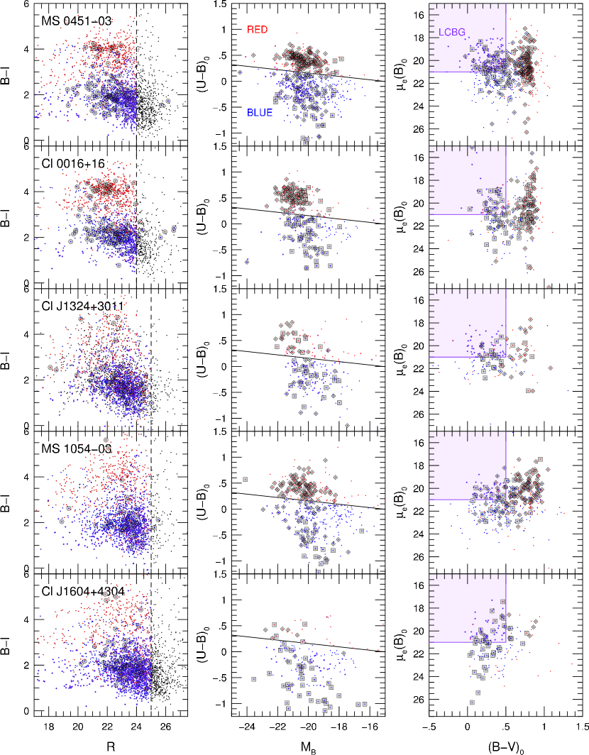
Figure 6: Photometric properties and sample definitions for objects in our 5 cluster fields. Each row is for the labeled cluster field. The left-hand column contains the apparent $B-I$, vs $R$ color-magnitude diagram. The characteristic sample limit for each cluster is marked by a vertical dashed line. Grey encircled points have secure spectroscopic redshifts from our survey. Center and right panels contain rest-frame $U-B$ and $B-V$ colors, respectively, versus $B$-band absolute magnitude and rest-frame $B$-band surface brightness within the half-light radius. Rest-frame quantities are based on best available redshifts. These panels illustrate the Red Sequence, Blue Cloud, and LCBG samples, defined in the text, for all galaxies with spectroscopic redshifts. Grey ensquared points are cluster objects sampled from our survey; grey diamonds are cluster objects from the literature.

In Figures 1-5, we present the projected sky distribution for our targets in each of our fields. Objects with secure spectroscopic measurements are indicated by blue diamonds. In each figure, we display an outline of the respective fields of view for the WIYN imaging and the DEIMOS spectroscopy along with the derived $R_{200}$ radius for the cluster. The distribution in color-magnitude space for our sources with successful spectroscopy can be seen in the left-hand panel of Figure 6.

4.2 Galaxy Classification

For all sources with WIYN photometry, we provide a photometric classification, which will be used in subsequent papers in this series to differentiate between various cluster populations. We divide cluster sources into the following classes: Red Sequence (RS), Blue Cloud (BC) and Luminous Compact Blue Galaxies (LCBGs). While RS and BC are exclusive classifications, LCBGs are a subset of the BC.

For the RS class, we adopt the definition originated by Willmer et al. (2006) and subsequently employed by Crawford et al. (2009). RS galaxies are defined as satisfying the following relation:

$$U-B>-0.032\times(M_{B}+21.52)+0.204.$$ (1)

This definition is based on a $-0.25$ mag shift in the zeropoint of the color-magnitude relationship at intermediate redshifts. BC galaxies are defined as all galaxies below this relationship. The distinction between the RS and BC classes is evident in the center panels of Figure 6.

Finally, the LCBG subset consists of the most compact and luminous members of the BC class such that they have the following rest-frame parameters: $(B-V)_{o}<0.5$, $\mu_{B}<21$ mag arcsec^-2, and $M_{B}<-18.5$ (Crawford et al. 2006). These parameters were defined to isolate “enthusiastic” star forming galaxies, i.e., luminous galaxies with active star formation ongoing for at least several hundred million years. This definition is slightly different than the one used in Werk et al. 2004 and Garland et al. 2004, where $(B-V)_{o}<0.6$. The differences between the definitions is minor, and adopting their definition would only increase our number densities by $8\%$. Heavily obscured objects will not be identified as LCBGs. Figure 6 shows our selection for LCBGs in terms of color and surface brightness.

5 Redshift Analysis

5.1 Completeness

In total, we attempted to measure spectra from 1288 slits over 15 masks. Table 6 summarizes our overall results. We were able to measure secure redshifts ($Q=-1$, 3, or 4) for 848 sources, thus yielding a total success rate of $66\%$. This is significantly below the $74\%$ success rate achieved in the Team Keck Redshift Survey (TKRS, Wirth et al. 2004), which used the same instrument with an exposure time of 3600 s per mask but with a lower-resolution grating yielding higher signal-to-noise. In our longer-exposure masks, we reach a comparable completeness level; thus, our lower completeness is primarily the result of higher resolution.

In Table 7, we list the success rate for determining a secure redshift ($Q\geq 3$) for each of the different masks. Our average success rate for the October 2005 run was $69\%$ vs. $60\%$ for the April 2006 observing run. The difference between the two runs can most likely be attributed to the higher redshift of the clusters in the latter run. The highest completeness fractions for the second run occur for the lowest redshift cluster in the group and for the mask with the longest exposure time.

5.2 Literature Data

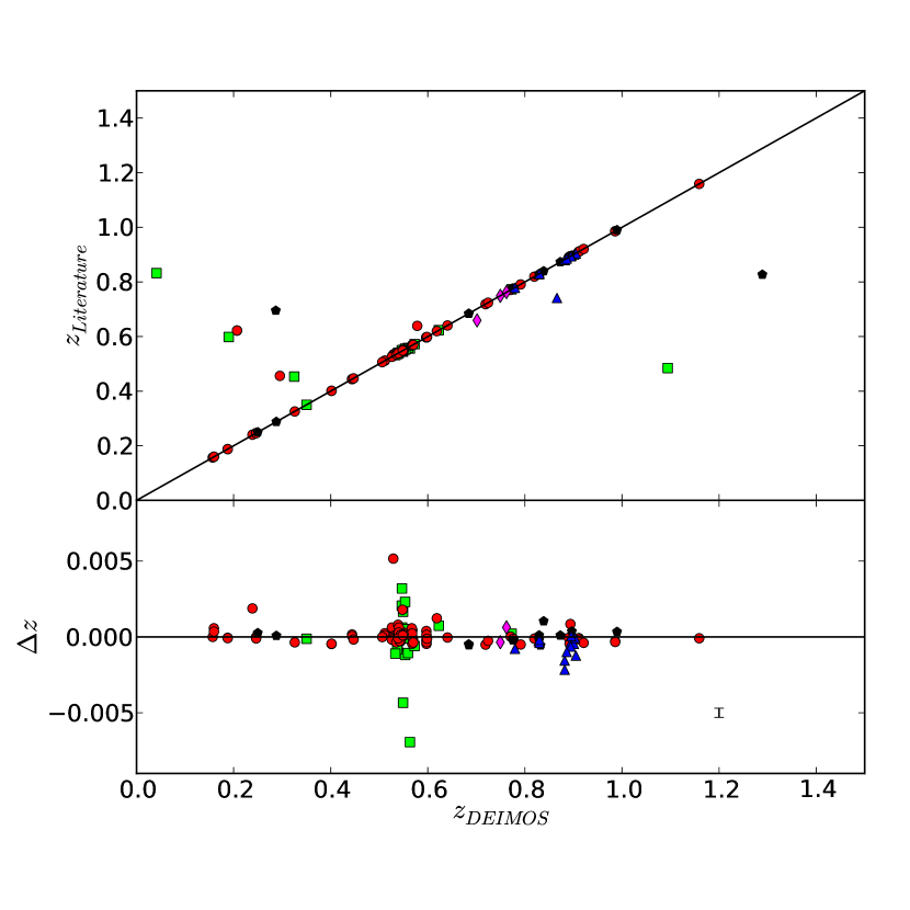
Figure 7: Spectroscopic redshifts measured from DEIMOS compared to literature sources. Different clusters are represented by red circles (MS 0451-03), green squares (Cl 0016+16), purple diamonds (Cl J1324+3011), black pentagons (MS 1054-03), and blue triangles (Cl 1604+4304). Excluding catastrophic outliers, the overall difference of the sample is $\Delta z=-0.00013$ with a dispersion of $\sigma_{z}=0.0011$. Sources with catastrophic errors are still included in this figure. A typical error bar for the sources is included in the bottom-right corner of the bottom panel.

Of our 848 galaxies with secure spectroscopic redshifts, 142 have spectroscopic redshifts from other sources in the literature. The vast majority of these redshifts (86 sources) are from DEIMOS spectroscopy in MS 0451-03 field by Moran et al. (2007). In Figure 7, we compare the independent measurements for these 142 sources; only a small number of significant outliers exist. We find that $91\%$ have redshifts that agree to within $|\Delta z|<0.005$, with only 12 measurements that have differences of $|\Delta z|\geq 0.005$. Excluding the outliers, we find the mean systematic difference between our redshifts and the literature results to be $\Delta z=-0.00013$ with a dispersion of $\sigma_{z}=0.0011$.

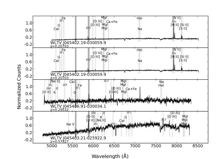
Figure 8: DEIMOS spectra from the MS 0451-03 field for objects with redshifts different from those reported in the literature. The spectra have been smoothed with a boxcar of length 4 Å and important features are described in the text. Grey regions highlight significant sky lines and the position of possible detected, individual spectral features are noted in the figure.

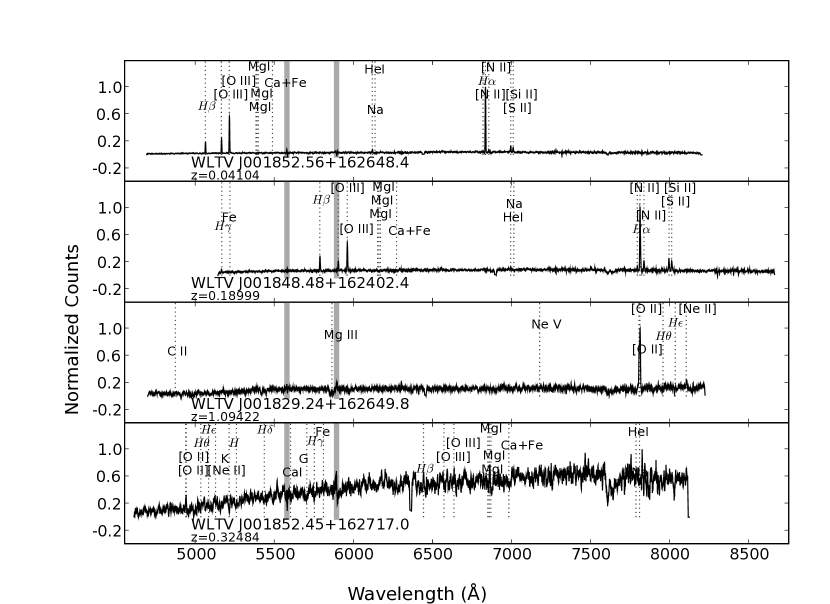
Figure 9: DEIMOS spectra from the Cl 0016+16 field for objects with redshifts different from those reported in the literature. The spectra have been smoothed with a boxcar of length 4 Å and important features are described in the text.

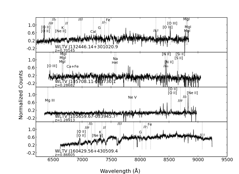
Figure 10: DEIMOS spectra from the other fields for objects with redshifts different from those reported in the literature. The spectra have been smoothed with a boxcar of length 4  Å and important features are described in the text.

The following 11 objects were identified as outliers (one source has two DEIMOS measurements). We present all twelve DEIMOS spectra in Figures 8-10.

WLTV J045402.19-030059.9: This source was identified as MS 0451.6-0305:PPP 1147 from Ellingson et al. (1998). The reported redshift for the source was $z=0.6219$. We observed this source on two different DEIMOS masks, and the very secure ($Q=4$) spectroscopic measurements for this source agree to within $\Delta z=0.00001$ of $z=0.20703$. The presence of H$\beta$, [O III]$\lambda 4959$,$\lambda 5007$, and H$\alpha$ confirm the redshift of this source. Due to limitations in the wavelength coverage, resolution, and signal-to-noise of the original spectrum, H$\alpha$ was not identified and [O III]$\lambda 5007$ was likely identified as [O II] $\lambda 3727$ leading to the erroneous redshift of $z=0.6219$.

WLTV J045406.91-030034.1: This source was identified as MS 0451.6-0305:PPP 1349 from Ellingson et al. (1998). The reported redshift for the source was $z=0.456$. We measure a very secure redshift of $z=0.29532$ based on several emission features. There is no obvious reason for the different redshift reported in the literature source, but the target lies in a crowded region and confusion is a possibility.

WLTV J045403.21-025922.9: This source was identified as MS 0451.6-0305:PPP 1790 by Ellingson et al. (1998). The reported redshift for the source was $z=0.6391$ and it was originally identified as an emission-line source. We obtained a very secure redshift measurement of $z=0.57827$ and identify the source as an absorption line system. The region is not very crowded, and there is no evident explanation for the $\Delta z=0.05$ discrepancy in redshift.

WLTV J001852.56+162648.4: This source was identified as MS 0015.9+1609:PPP 1160 from Ellingson et al. (1998). Most likely, H$\alpha$ was misidentified as [O II] $\lambda 3727$ at $z=0.83226$. We derive a redshift of $z=0.041038$ due to detecting H$\alpha$ and [O III]$\lambda 5007$ in the spectrum.

WLTV J001848.48+162402.4: This source was identified as MS 0015.9+1609:PPP 405 from Ellingson et al. (1998). Most likely, H$\alpha$ was misidentified as [O III]$\lambda 5007$ at $z=0.587$. We measure the redshift as $z=0.18998$ due to detecting H$\alpha$ and [O III]$\lambda 5007$ in the spectrum.

WLTV J001829.24+162649.8: This source was identified as MS 0015.9+1609:PPP 1150 from Ellingson et al. (1998). The reported redshift for the source was $z=0.48463$. We believe the redshift is $z=1.09422$ based on resolving the [O II] $\lambda 3727$ doublet which was likely not visible in the original spectrum.

WLTV J001852.45+162717.0: This source was matched with MS 0015.9+1609:PPP 1317 from Ellingson et al. (1998). The reported redshift for the source was $z=0.4533$. There was no obvious reason for the difference between our measured value of $z=0.32484$ and the value from the literature although we have a very secure ($Q=4$) measurement of the redshift based on detection of the [O II] $\lambda 3727$ doublet and H$\beta$.

WLTV J132446.14+301020.9: This source was matched with Cl J1324+3011 1636 from Postman et al. (2001). The reported redshift was $z=0.659$. We detect very strong [O II] $\lambda 3727$ measured at $z=0.70145.$ There is no obvious reason for the difference but the source is in a crowded region and may be misidentified.

WLTV J105708.11-R033730.1: This source was matched with MS J1054-0321 H7758 from Tran et al. (2007). The reported redshift for this source was $z=0.6952$. We measure a secure redshift of $z=0.28682$ via several emission lines. It lies in a crowded region of the field and may be mis-identified.

WLTV J105659.67-033945.7: This source corresponds to MS J1054-0321 K556 from Tran et al. (2007). There are no strong emission lines for this object and it is relatively faint at $R=23.45$. We measured $z=0.289$ as compared to $z=0.827$ from Tran et al. In both surveys, it has a quality of only $Q=3$ and likely a marginal detection.

WLTV J160429.56+430509.4: This source was matched with Cl J1604+4304 3197 from Postman et al. (2001). The reported redshift for this source was $z=0.7415$. We measure $z=0.86605$. Our spectrum of the source reveals a very strong absorption line system, although it could be blended with another source.

For the eleven discrepant redshifts, seven are from Ellingson et al. (1998). As compared to their CFHT MOS observations, the DEIMOS spectra exhibit higher signal-to-noise, greater wavelength coverage, and improved resolution. This allows us to de-blend the [O II] $\lambda 3727$ doublet for secure redshift measures as well as to identify other emission lines out to higher redshift. Overall, we find that only one of our redshift measurements among these discrepant sources is marginal, whereas the other ten are very secure measurements with either the [O II] $\lambda 3727$ doublet resolved or multiple lines identified in the spectrum. Four of the sources are either blended or in crowded regions of the field and they could be mis-identified with other sources in either our survey or the previous ones.

5.3 Accuracy of Photometric Redshifts

We now compare our spectroscopic redshifts to the photometric redshift measurements from Crawford et al. (2009). The photometric redshifts were measured using a hybrid method (Csabai et al. 2003) that combines the template method (Koo 1985) and training-set method (Connolly et al. 1995). After creating a grid of artificial spectral energy distributions based on the models of Bruzual & Charlot (2003) that cover a range of star formation histories, we adjusted the grid in flux space according to the measured colors of known spectroscopic sources. Finally, photometric redshifts were calculated using all of our flux measurements, including the narrow-band observations, on this new grid. Since each cluster was observed with an unique set of narrow band filters, each cluster has its own unique grid, which was originally based on the same set of models. This method corrects for the effects of incomplete coverage in color space by the models along with any minor effects introduced by offsets in photometric calibration.

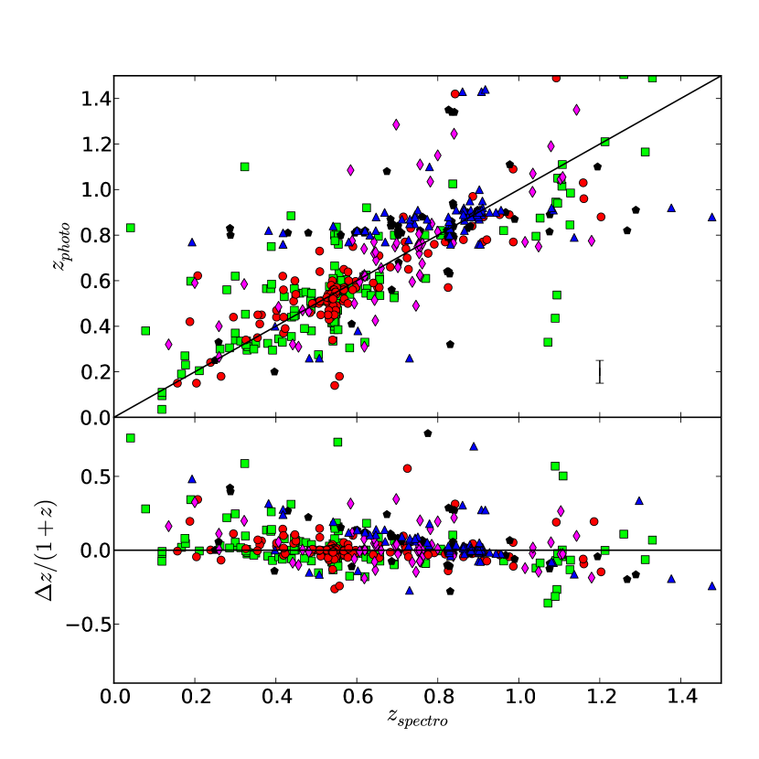
Figure 11: Photometric redshift compared to spectroscopic redshift excluding sources in our original training set data. Symbols are the same as in Figure 7. Sources with catastrophic errors are still included in this figure. A typical error bar for the sources is included in the bottom-right corner of the top panel.

In Figure 11, we plot the spectroscopic redshifts versus the photometric redshifts for all sources with spectroscopic redshifts, excluding those used in the original training set. For the most part, the clusters do not show any major systematic errors and the overall bias in the sample is relatively small. The overall sample has systematic errors of $\delta z/(1+z)=0.0015$ and random error of $\sigma_{z}/(1+z)=0.07$ with $10\%$ of the sample being catastrophic outliers (defined as objects with discrepancies larger than $3\sigma_{z}$). These results are consistent with other studies (Ilbert et al. 2006, Erben et al. 2009) of similar data quality. The sources with the largest errors are those which have been identified as AGN; we did not include any AGN templates in our original model grids and thus could not derive accurate redshifts for this class of galaxies.

One cluster, Cl J1604+4304, does show fairly substantial systematic errors, especially for lower-redshift sources. These sources are predominately faint, blue galaxies that have been assigned photometric redshifts closer to the cluster redshift than would be appropriate. After re-examining the training set, we found that this systematic error resulted from the inclusion of a cluster AGN source in the training set. The colors of the AGN were similar to those of low-redshift blue galaxies and this, along with the small number of blue galaxies in the original training set, caused the model grid to be distorted in an unrealistic manner. However, this highlights a limitation in this method such that the measured photometric redshifts are only as good as the training set that is used. For future analysis using the photometric redshifts, we plan to recalculate the model grids using all data now available.

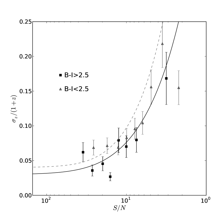
Figure 12: Random error in photometric redshifts as a function of signal to noise for red ($B-I>2.5$) and blue ($B-I<2.5$) sources. For red sources, each point represents the average of 20 sources; for blue, 40 sources. The points are in good agreement with the predictions for red (solid line) and blue (dotted line) galaxies based on our photometric errors.

To illustrate the importance of photometric errors on the photometric redshift measurements, we present the random error for the entire sample as a function of signal-to-noise in the $R$-band in Figure 12. We show the data for red and blue objects as defined by their apparent $B-I$ colors. For comparison, we plot the expected random error as a function of signal to noise for two spectral energy distributions representing a red and blue galaxy assuming photometric errors typical of our WIYN observations. Although there is significant scatter around these models, the data behave as suggested by the models with a lower limit of $\sigma_{z}=0.03$ in error for red sources and $\sigma_{z}=0.05$ for blue sources and then increasing rapidly for sources with signal to noise less than 10 in the $R$-band.

6 Luminous Compact Blue Galaxies in Clusters

The initial impetus for this study was to determine the number density and distribution of LCBGs in intermediate-redshift galaxy clusters. Crawford et al. (2006) found evidence for a large enhancement of the population of LCBGs using photometric measurements. Here, we can confirm their presence with spectroscopic measurements.

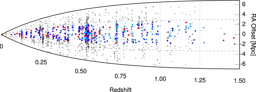
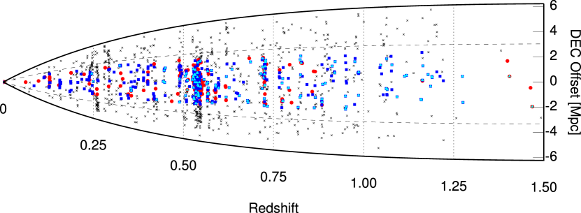
Figure 13: “Wedge” diagrams for the MS0451-03 field. (a) Projected spatial offset in the RA axis [Mpc] from the cluster center (defined by the BCG) among targets in the field. (b) Projected spatial offset in the Dec axis [Mpc] from the cluster center among targets in the field. Red symbols correspond to galaxies classified as red sequence; similarly, blue symbols show the blue cloud class, cyan represents the LCBG class, and small black crosses indicate additional, unclassified objects with good redshifts. The horizontal dashed curves indicate the extent of the DEIMOS survey field.

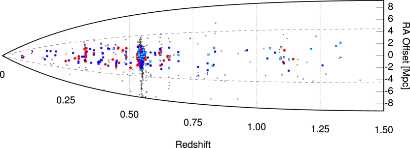
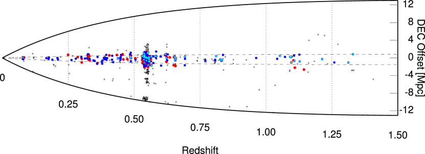
Figure 14: “Wedge” diagrams for the Cl 0016+16 field. Symbols as in Fig. 13.

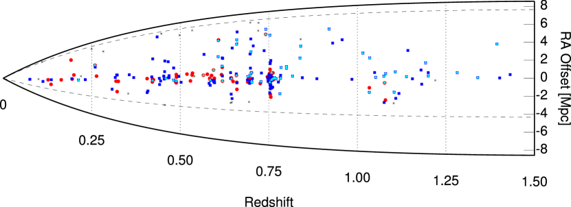
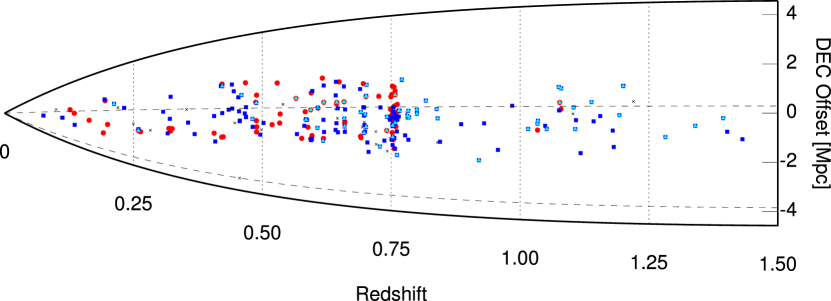
Figure 15: “Wedge” diagrams for the w08 field. Symbols as in Fig. 13.

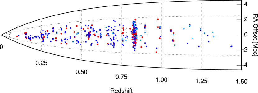
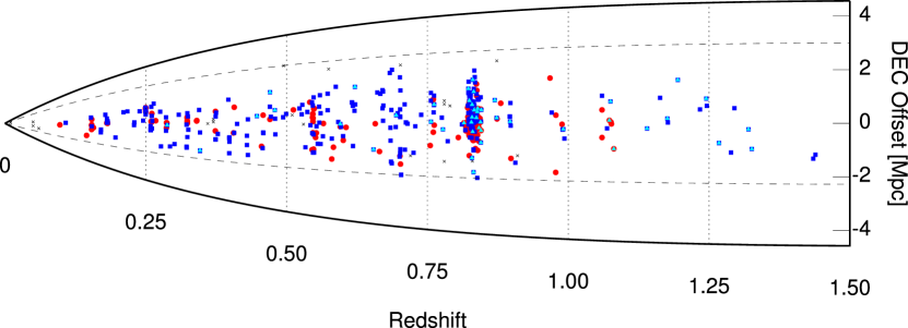
Figure 16: “Wedge” diagrams for the w07 field. Symbols as in Fig. 13.

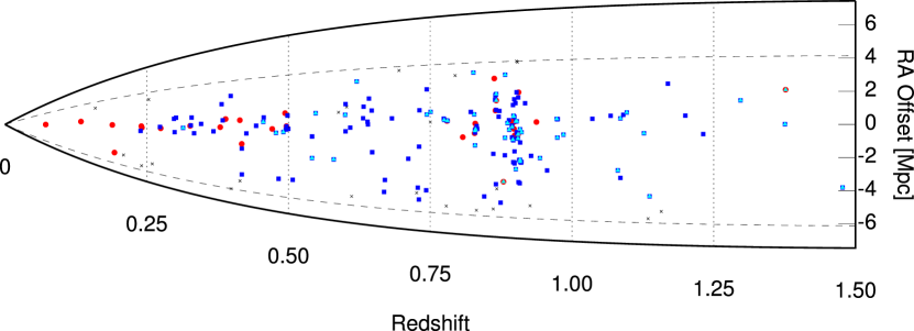
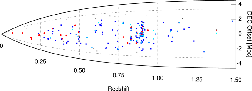
Figure 17: “Wedge” diagrams for the w10 field. Symbols as in Fig. 13.

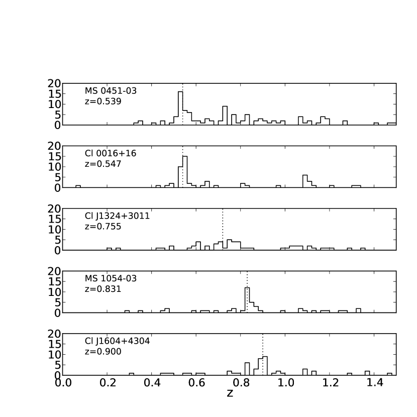
Figure 18: The redshift distribution for LCBGs in the five clusters. The number counts are limited to within $R_{200}$ of each respective cluster center. For all the clusters, an increase in the number of LCBGs is noticed at the cluster redshift (indicated by a dotted vertical line).

In Figures 13-17, we plot the spatial distribution of different classes of objects in each of our five survey fields. The strong clustering for LCBGs which is implied in these figures is further demonstrated in the redshift histograms of LCBGs presented in Figure 18. A peak in the LCBG distribution can be seen at the redshift of each cluster with the most distinct peaks occurring at the more massive clusters. As shown previously in Crawford et al. (2006), this is further evidence that the presence of LCBGs correlates with galaxy density.

From our spectroscopy, we identify 145 LCBGs, of which 56 are within the projected $R_{200}$ radius of the cluster center and $|\Delta z|\leq 0.03$ of the cluster redshift. From these measurements, we can estimate the density of LCBGs within $R_{200}$ of the cluster. To account for spectroscopic incompleteness, we estimated the number of possible cluster LCBGs based on the photometric measurements and assuming each object was at the redshift of the cluster. Using the spectroscopic sources for each cluster, we measured the fraction of photometrically-determined cluster LCBGs that were bona fide cluster LCBGs. For the high redshift cluster, our photometric data includes all sources within $R_{200}$; for the low redshift clusters, we have to apply a second correction to account for not sampling the entire region out to $R_{200}$. For the two low-redshift clusters, we calculate the volume within $R_{200}$ being sampled by the photometric data and correct the density by this fraction. If we assume a volume for each of our clusters given by a sphere with a radius of $R_{200}$, we would find a space density for LCBGs in clusters ranging from $1.65\pm 0.25$ Mpc^-3 at $z=0.55$ to $3.13\pm 0.65$ Mpc^-3 at $z=0.8$.

In comparison, the field number density of LCBGs also rapidly rises with redshift with the number density increasing from $1.2\times 10^{-3}$ Mpc^-3 at $z=0.5$ to $9\times 10^{-3}$ Mpc^-3 at $z=0.9$ for a similarly defined sample (Phillips et al. 1997). Following the same procedure as Phillips et al. (1997), we can calculate the density of field LCBGs over those two redshift ranges by using our non-cluster sample. We calculate field densities of $1.8\pm 0.3\times 10^{-3}$Mpc^-3 at $z=0.5$ and $7.5\pm 1.2\times 10^{-3}$ Mpc^-3 at $z=0.9$ for field LCBGs, which are very similar to the Phillips et al. measurements. For the low redshift calculations, we used the Cl J1324+3011, MS 1054-03, and Cl J1604+4304 fields; for the high redshift, MS 0451-03 and Cl 0016+16 fields. We adopt the Phillips et al. (1997) values due to the better spectroscopic completeness in their data for the high redshift field samples; however, this choice does not significantly change our results presented here.

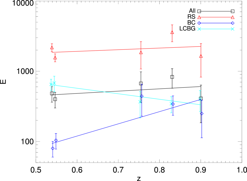
Figure 19: Enhancement factor $E$ as a function of redshift $z$ for the five clusters in our sample, for red sequence galaxies (RS), blue cloud objects (BC), luminous compact blue galaxies (LCBG), and all types together. The value of $E$ is defined as the relative density of a given galaxy type in the cluster vs. the field at a given redshift. The indicated line for each class represents a linear fit to $\log(E)$ as a function of $z$, accounting for the measurement errors. The RS class shows little evolution in $E$ within our sample. The relative BC population density rises significantly with increasing redshift. The corresponding LCBG population density relative to the field displays the opposite behavior, decreasing strongly as redshift increases and thus suggesting strong differential evolution in the BC and LCBG populations.

Since the cluster space density depends on the richness of the selected cluster, to make sense of the differences between the cluster and the field we compute an enhancement, $E$, defined as the ratio of cluster to field density. LCBGs have an average enhancement of $E=749\pm 116$ at $z=0.55$ and $E=416\pm 95$ at $z=0.8$. For comparison, the enhancement of red sequence galaxies can be calculated from their field (Willmer et al. 2006) and cluster (Crawford et al. 2009) luminosity functions. At $z=0.55$ ($0.80$), red sequence galaxies have an enhancement of $E=1872\pm 174$ ($2369\pm 500$). Using the measured blue fraction in each cluster, we can estimate the enhancement of BC galaxies to be $E=92\pm 12$ ($344\pm 78$) and for all types of galaxies to be $E=440\pm 78$ ($636\pm 173$) at $z=0.55$ ($0.8$), respectively. The enhancement for RS, BC, and LCBGs for each cluster are given in Table 8, and the change with redshift of the enhancement for each class of objects can be seen in Figure 19.

At intermediate redshifts of $z=0.5$, these results indicate that LCBGs are preferentially found in high-density environments relative to the overall star-forming population. Although they are not as strongly clustered as red galaxies (by a factor of 3), they are $1.5$ times as clustered as the overall galaxy distribution and seven times more clustered than regular blue cloud galaxies in general. At higher redshifts, LCBGs also had a high density of objects in clusters, but the field density of LCBGs was significantly higher (Guzman et al. 1997). This results in a factor of two lower LCBG enhancement at this earlier epoch. This is remarkable because the enhancement of blue galaxies is a factor of 3.5 higher at $z=0.8$, thereby equalizing the enhancement of blue and LCBG populations at a redshift where there is a large fraction of LCBGs in the blue field population. In other words, there is a very strong differential evolution of subsets of the blue galaxy population between clusters and the field between a redshift of $z=0.8$ to $z=0.5$.

Cluster blue galaxies are assumed to be an infalling field population which is extinguished by different processes in the cluster (Dressler et al. 1997; Balogh, Navarro, & Morris 2000; Ellingson et al. 2001, Bravo-Alfaro et al. 2001, Chung et al. 2009). If we assume the same is true for LCBGs, we would expect their number density to follow a similar pattern to either the overall population or the BC population, which is the case for our higher redshift clusters. For the $z\sim 0.55$ clusters, we find a much higher number of LCBGs than we would predict from this simple model. In these clusters, LCBGs are completely absent in the very high-density cores of the clusters (Crawford et al. 2006). This is strong evidence that the cluster environment is triggering the starburst in these galaxies (Porter et al. 2008; Mahajan, Haines, and Raychaudhury 2011).

In the original work (Crawford et al. 2006), we couched the enhancement as a way to connect different galaxy populations by their morphology-density relationship. Low-redshift dwarf spheroidal galaxies, which Koo et al. (1994) originally proposed as a possible descendant of LCBGs, have a similar enhancement to the intermediate-redshift LCBGs. However, the higher-redshift LCBGs are likely a more heterogeneous population and their evolutionary path is more complex (Phillips et al. 1997, Noeske et al. 2006). Hence, more detailed information about the individual objects will be needed to connect these cluster objects with their lower-redshift cluster relatives. Nonetheless, our findings here on enhancement bear out our earlier results based on photometric redshifts alone.

Unlike field LCBGs (Guzman et al. 1997), cluster LCBGs show only a modest decrease in number density with redshift. As compared to RS and BC galaxies, LCBGs are the only group that shows an increase in the enhancement with decreasing redshift as seen in Figure 19. This study shows that massive clusters at intermediate redshifts still contain a relative abundance of LCBGs despite their increasing rarity in the field, perhaps because the cluster periphery is a fertile environment for triggering the LCBG phase in in-falling gas-rich galaxies. The clusters in our survey are representative of the most massive systems in the Universe. As seen in the comparison between Abell 851 and MS 1512.4+3647 (Lotz et al. 2003), the extreme environment in massive systems may lead to very different properties than the more common, lower mass systems. It will be important to broaden this type of investigation to a range of environments and redshifts to further explore the triggering of LCBGs. Furthermore, confirmation of this trend is still required at low redshifts where field LCBGs are almost non-existent (Werk et al. 2004). Future studies targeting the periphery of low-redshift, rich galaxy clusters could confirm whether this trend continues to today.

7 Summary

We have presented the spectroscopic observations of blue galaxies in five moderate-to-high redshift galaxy clusters. The five clusters targeted here include some of the most massive systems at their respective redshifts and we have preferential targeted blue sources associated with the clusters. This paper is the first in a series attempting to determine a complete census of the properties of optical star-forming galaxies in intermediate-redshift galaxy clusters.

We have detailed the DEIMOS spectroscopic observations for blue galaxies selected from a deep, multi-band imaging survey with the WIYN 3.5 m telescope. This includes the object selection, observations, data reduction, and analysis. In addition, we present a table of the measurements for all 1288 sources that were targeted as part of this survey including spectroscopic redshift and photometric classification.

We determined secure redshifts for 848 sources. Our success rate for determining the redshift for sources is comparable to previous studies with the same instrument and telescope. In our sample, 142 sources have redshifts previously reported in the literature. Twelve measurements (11 sources) are discrepant with the literature values, although redshifts are very securely ($Q=4$) determined for ten of these sources. Overall, our results show excellent agreement with the previously-published results. Comparing the spectroscopic redshifts to our previously-measured photometric measurements yields results that confirm the high quality of our photometric measurements. Photometric redshifts from one cluster did exhibit systematic errors for low-redshift blue sources, which we attribute to AGN contamination in the original training set. The overall dispersion in the measurement is comparable to our expectations from modeling our photometric errors.

We have estimated the number density of LCBGs in these five galaxy clusters based on our new spectroscopic identifications. By examining the number distribution of LCBGs as a function of redshift, we find the clusters to be rich in LCBGs with a relative enhancement over the field population of a factor of 500, roughly 2.5 times larger than the enhancement of the general blue cluster population. The relative enhancement between sub-populations of star-forming galaxies diverges between $z=0.8$ to $z=0.5$ such that LCBGs become relatively more common in massive clusters at more recent epochs. This overdensity of luminous compact star-forming galaxies indicates that the cluster environment, while generally accelerating the transformation of galaxies from the blue cloud to the red sequence, is somehow better able to nurture or sustain the LCBG phase relative to the field.

Table 1: Summary of Fields

Field	WLTV ID	$\alpha$	$\delta$	$z$	$\sigma(z)$	$M_{200}$	$R_{200}$	$R_{200}$
		(J2000)	(J2000)		(km s-1)	($10^{1}5M_{\odot}$)	(Mpc)	($\arcsec$)
MS 0451-03	w05	04:54:10.8	$-$03:00:51	0.5389	1328	3.00	2.45	386
Cl 0016+16	w01	00:18:33.6	$+$16:26:16	0.5467	1490	4.22	2.74	428
Cl J1324+3011	w08	13:24:48.8	$+$30:11:39	0.7549	806	0.59	1.31	178
MS 1054-03	w07	10:56:60.0	$-$03:37:36	0.8307	1105	1.45	1.72	225
Cl J1604+4304	w10	16:04:24.0	$+$43:04:39	0.9005	1106	1.40	1.65	211

Table 2: Slitmask Design Data

No.	Mask Name	$\alpha$	$\delta$	PA
		(J2000)	(J2000)	($\arcdeg$)
1	w01.m1	00 18 33.63	16 26 30.0	270
2	w01.m2	00 18 33.63	16 26 30.0	270
3	w01.m3	00 18 33.63	16 26 30.0	270
4	w01.m4	00 18 33.63	16 26 30.0	270
5	w05.m1	04 54 10.81	$-$03 00 56.9	45
6	w05.m2	04 54 10.81	$-$03 00 56.9	45
7	w05.m3	04 54 10.81	$-$03 00 56.9	315
8	w05.m4	04 54 10.81	$-$03 00 56.9	315
9	w07.m1	10 56 59.09	$-$03 38 02.8	41
10	w07.m3	10 57 03.33	$-$03 36 54.2	320
11	w08.m1	13 25 03.53	30 10 54.0	270
12	w08.m2	13 25 03.53	30 10 54.0	270
13	w10.m1	16 04 21.16	43 04 10.9	41
14	w10.m2	16 04 19.26	43 04 05.2	41
15	w10.m3	16 04 20.40	43 04 57.0	320

Table 3: Slitmask Observation Data

No.	Mask	Obs. Date	Int. Time	Grating	Blaze	Filter	$\lambda_{c}$	$\lambda$ range
		(UT)	(s)	(l mm-1)	(Å)		(Å)	(ÅÅ)
1	w01.m1	2005 Nov 03	4800	900	5500	GG455	6500	4700–8300
2	w01.m2	2005 Nov 03	3600	900	5500	GG455	6500	4700–8300
3	w01.m3	2005 Nov 03	3600	900	5500	GG455	6500	4700–8300
4	w01.m4	2005 Nov 03	3600	900	5500	GG455	6500	4700–8300
5	w05.m1	2005 Nov 03	3600	900	5500	GG455	6500	4700–8300
6	w05.m2	2005 Nov 03	3600	900	5500	GG455	6500	4700–8300
7	w05.m3	2005 Nov 03	3600	900	5500	GG455	6500	4700–8300
8	w05.m4	2005 Nov 03	3600	900	5500	GG455	6500	4700–8300
9	w07.m1	2007 Apr 17	3600	1200	7760	OG550	7800	6450–9150
10	w07.m3	2007 Apr 17	3600	1200	7760	OG550	7800	6450–9150
11	w08.m1	2007 Apr 17	3600	1200	7760	OG550	7500	6150–8850
12	w08.m2	2007 Apr 17	3600	1200	7760	OG550	7500	6150–8850
13	w10.m1	2007 Apr 17	3600	1200	7760	OG550	8000	6650–9350
14	w10.m2	2007 Apr 17	3600	1200	7760	OG550	8000	6650–9350
15	w10.m3	2007 Apr 17	4800	1200	7760	OG550	8000	6650–9350

Table 4: WLTV DEIMOS Catalog

Table 5: WLTV DEIMOS Catalog

ID	$\alpha$	$\delta$	$R$	Mask	Slit	$z$	$Q$	$z_{\mbox{lit}}$	Ref	Class
	(J2000)	(J2000)	(mag)
(1)	(2)	(3)	(4)	(5)	(6)	(7)	(8)	(9)	(10)	(11)
WLTV J045352.64-030353.4	73.4693271	-3.0648573	19.28	w05.m1	0	0.41676	4	…	…	BC
WLTV J045355.35-030636.1	73.4806362	-3.1100513	19.54	w05.m1	2	0.25792	4	…	…	RS
WLTV J045353.13-030625.5	73.4713687	-3.1071082	22.32	w05.m1	3	0.89036	4	0.89030	5	BC
WLTV J045353.84-030600.8	73.4743266	-3.1002444	21.76	w05.m1	4	0.54157	4	…	…	BC
WLTV J045354.32-030451.0	73.4763465	-3.0808360	21.27	w05.m1	5	0.58863	3	…	…	BC
WLTV J045354.48-030518.1	73.4769991	-3.0883711	23.91	w05.m1	6	0.77239	2	…	…	BC
WLTV J045355.23-030555.3	73.4801383	-3.0986969	21.98	w05.m1	7	0.56637	4	…	…	BC
WLTV J045356.11-030346.2	73.4837898	-3.0628533	21.39	w05.m1	8	0.56693	4	0.56750	2	BC

Note. — (1) Identification in WLTV survey (2) Right Ascension (3) Declination (4) R mag (5) Mask (6) Slit (7) Redshift (8) Redshift quality (9) Literature redshift (10) Reference (11) Photometric classification.

Table 6: Redshift Quality Distribution

$Q$	Definition	$N_{obj}$	$F_{obj}$
4	Very secure redshift ($P>99\%$); at least two spectral features identified	550	0.428
3	Secure redshift ($P>95\%$); one strong line and another weak feature identified or single wide line	177	0.138
2	Uncertain redshift; signal is present but no unambiguous spectral line identified	85	0.066
1	No redshift; $S/N$ too poor	290	0.225
$-1$	Star	121	0.094
$-2$	No redshift measured because of instrumental artifacts in spectrum	56	0.043

Table 7: Slitmask Results

No.	Mask Name	$N_{o}$	$N_{z}$	$F_{z}$
				(%)
1	w01.m1	93	69	74
2	w01.m2	90	59	67
3	w01.m3	89	58	65
4	w01.m4	87	57	66
5	w05.m1	93	67	73
6	w05.m2	90	52	58
7	w05.m3	90	70	77
8	w05.m4	89	64	71
9	w07.m1	79	40	51
10	w07.m3	64	31	48
11	w08.m1	87	58	68
12	w08.m2	85	65	77
13	w10.m1	82	49	61
14	w10.m2	72	35	50
15	w10.m3	73	48	66

Table 8: Enhancement in each cluster

Cluster	z	All	RS	BC	LCBG
MS 0451-03	$0.5389$	$483\pm 120$	$2180\pm 283$	$80\pm 20$	$786\pm 156$
Cl 0016+16	$0.5467$	$400\pm 100$	$1564\pm 203$	$104\pm 26$	$712\pm 174$
Cl J1324+3011	$0.7549$	$670\pm 310$	$1857\pm 780$	$442\pm 212$	$574\pm 246$
MS 1054-03	$0.8307$	$830\pm 257$	$3600\pm 972$	$341\pm 105$	$326\pm 78$
Cl J1604+4304	$0.9005$	$410\pm 225$	$1650\pm 825$	$250\pm 137$	$348\pm 122$

Figure 1: Projected sky distribution for targets in the MS 0451-03 field. Dotted box indicates the approximate field-of-view of the WIYN photometry from which the photometric redshifts were derived. Solid polygon indicates the field-of-view of the DEIMOS spectroscopy from this work. Dashed circle indicates the $R_{200}$ radius for this cluster. Green pluses represent objects with WIYN photometry. Cyan circles denote targets with previously-published redshifts appearing in the literature. Red crosses specify objects targeted with DEIMOS that did not yield a secure redshift measurement. Blue diamonds correspond to galaxies with secure DEIMOS redshifts. Yellow symbols identify stars. The figure is only available in high-resolution version.

Figure 2: Projected sky distribution for targets in Cl 0016+16 field. Symbols as in Fig. 1. The figure is only available in high-resolution version.

Figure 3: Projected sky distribution for targets in Cl J1324+3011 field. Symbols as in Fig. 1. The figure is only available in high-resolution version.

Figure 4: Projected sky distribution for targets in MS 1054-03 field. Symbols as in Fig. 1. The figure is only available in high-resolution version.

Figure 5: Projected sky distribution for targets in Cl J1604+4304 field. Symbols as in Fig. 1. The figure is only available in high-resolution version.

References

- Balogh et al. (2000) Balogh, M. L., Navarro, J. F., & Morris, S. L. 2000, ApJ, 540, 113
- Barger et al. (1996) Barger, A. J., Aragon-Salamanca, A., Ellis, R. S., Couch, W. J., Smail, I., & Sharples, R. M. 1996, MNRAS, 279, 1
- Boselli & Gavazzi (2006) Boselli, A., & Gavazzi, G. 2006, PASP, 118, 517
- Bravo-Alfaro et al. (2001) Bravo-Alfaro, H., Cayatte, V., van Gorkom, J. H., & Balkowski, C. 2001, A&A, 379, 347
- Bruzual & Charlot (2003) Bruzual, G., & Charlot, S. 2003, MNRAS, 344, 1000
- Butcher & Oemler (1978) Butcher, H., & Oemler, A., Jr. 1978, ApJ, 219, 18
- Butcher & Oemler (1984) Butcher, H., & Oemler, A., Jr. 1984, ApJ, 285, 426
- Carlberg et al. (1996) Carlberg, R. G., Yee, H. K. C., Ellingson, E., Abraham, R., Gravel, P., Morris, S., & Pritchet, C. J. 1996, ApJ, 462, 32
- Chung et al. (2009) Chung, A., van Gorkom, J. H., Kenney, J. D. P., Crowl, H., & Vollmer, B. 2009, AJ, 138, 1741
- Clowe et al. (2000) Clowe, D., Luppino, G. A., Kaiser, N., & Gioia, I. M. 2000, ApJ, 539, 540
- Connolly et al. (1995) Connolly, A. J., Csabai, I., Szalay, A. S., Koo, D. C., Kron, R. G., & Munn, J. A. 1995, AJ, 110, 2655
- Connolly et al. (1996) Connolly, A. J., Szalay, A. S., Koo, D., Romer, A. K., Holden, B., Nichol, R. C., & Miyaji, T. 1996, ApJ, 473, L67
- Cooper et al. (2008) Cooper, M. C., et al. 2008, MNRAS, 383, 1058
- Couch & Sharples (1987) Couch, W. J., & Sharples, R. M. 1987, MNRAS, 229, 423
- Cowie & Hu (1998) Cowie, L. L., & Hu, E. M. 1998, AJ, 115, 1319
- Crawford (2006) Crawford, S. M. 2006, Ph.D. Thesis
- Crawford et al. (2006) Crawford, S. M., Bershady, M. A., Glenn, A. D., & Hoessel, J. G. 2006, ApJ, 636, L13
- Crawford et al. (2009) Crawford, S. M., Bershady, M. A., & Hoessel, J. G. 2009, ApJ, 690, 1158
- Csabai et al. (2003) Csabai, I., et al. 2003, AJ, 125, 580
- Davis et al. (2003) Davis, M., et al. 2003, Proc. SPIE, 4834, 161
- Davis et al. (2007) Davis, M., et al. 2007, ApJ, 660, L1
- de Boor (1978) de Boor, C., 1978, A Practical Guide to Splines. (1st Ed; Berlin; Springer-Verlag)
- Donahue et al. (1998) Donahue, M., Voit, G. M., Gioia, I., Lupino, G., Hughes, J. P., & Stocke, J. T. 1998, ApJ, 502, 550
- Donahue et al. (2003) Donahue, M., Gaskin, J. A., Patel, S. K., Joy, M., Clowe, D., & Hughes, J. P. 2003, ApJ, 598, 190
- Dressler (1980) Dressler, A. 1980, ApJ, 236, 351
- Dressler & Gunn (1982) Dressler, A., & Gunn, J. E. 1982, ApJ, 263, 533
- Dressler & Gunn (1983) Dressler, A., & Gunn, J. E. 1983, ApJ, 270, 7
- Dressler et al. (1997) Dressler, A., et al. 1997, ApJ, 490, 577
- Dressler et al. (1999) Dressler, A., Smail, I., Poggianti, B. M., Butcher, H., Couch, W. J., Ellis, R. S., & Oemler, A. J. 1999, ApJS, 122, 51
- Duc & Bournaud (2008) Duc, P.-A., & Bournaud, F. 2008, ApJ, 673, 787
- Ellingson et al. (1998) Ellingson, E., Yee, H. K. C., Abraham, R. G., Morris, S. L., & Carlberg, R. G. 1998, ApJS, 116, 247
- Ellingson et al. (2001) Ellingson, E., Lin, H., Yee, H. K. C., & Carlberg, R. G. 2001, ApJ, 547, 609
- Erben et al. (2009) Erben, T., et al. 2009, A&A, 493, 1197
- Fadda et al. (1996) Fadda, D., Girardi, M., Giuricin, G., Mardirossian, F., & Mezzetti, M. 1996, ApJ, 473, 670
- Finn et al. (2004) Finn, R. A., Zaritsky, D., & McCarthy, D. W., Jr. 2004, ApJ, 604, 141
- Finn et al. (2008) Finn, R. A., Balogh, M. L., Zaritsky, D., Miller, C. J., & Nichol, R. C. 2008, ApJ, 679, 279
- Gal & Lubin (2004) Gal, R. R., & Lubin, L. M. 2004, ApJ, 607, L1
- Gallazzi et al. (2009) Gallazzi, A., et al. 2009, ApJ, 690, 1883
- Garland et al. (2004) Garland, C. A., Pisano, D. J., Williams, J. P., Guzmán, R., & Castander, F. J. 2004, ApJ, 615, 689
- Gioia & Luppino (1994) Gioia, I. M., & Luppino, G. A. 1994, ApJS, 94, 583
- Gioia et al. (2004) Gioia, I. M., Braito, V., Branchesi, M., Della Ceca, R., Maccacaro, T., & Tran, K.-V. 2004, A&A, 419, 517
- Gómez et al. (2003) Gómez, P. L., et al. 2003, ApJ, 584, 210
- Goto et al. (2005) Goto, T., et al. 2005, ApJ, 621, 188
- Guhathakurta et al. (1990) Guhathakurta, P., Tyson, J. A., & Majewski, S. R. 1990, ApJ, 357, L9
- Gunn et al. (1986) Gunn, J. E., Hoessel, J. G., & Oke, J. B. 1986, ApJ, 306, 30
- Guzman et al. (1996) Guzman, R., Koo, D. C., Faber, S. M., Illingworth, G. D., Takamiya, M., Kron, R. G., & Bershady, M. A. 1996, ApJ, 460, L5
- Guzman et al. (1997) Guzman, R., Gallego, J., Koo, D. C., Phillips, A. C., Lowenthal, J. D., Faber, S. M., Illingworth, G. D., & Vogt, N. P. 1997, ApJ, 489, 559
- Haines et al. (2009) Haines, C. P., et al. 2009, ApJ, 704, 126
- Halliday et al. (2004) Halliday, C., et al. 2004, A&A, 427, 397
- Hammer et al. (2001) Hammer, F., Gruel, N., Thuan, T. X., Flores, H., & Infante, L. 2001, ApJ, 550, 570
- Ilbert et al. (2006) Ilbert, O., et al. 2006, A&A, 457, 841
- Jee et al. (2005) Jee, M. J., White, R. L., Ford, H. C., Blakeslee, J. P., Illingworth, G. D., Coe, D. A., & Tran, K.-V. H. 2005, ApJ, 634, 813
- Jeltema et al. (2001) Jeltema, T. E., Canizares, C. R., Bautz, M. W., Malm, M. R., Donahue, M., & Garmire, G. P. 2001, ApJ, 562, 124
- Kocevski et al. (2009) Kocevski, D. D., Lubin, L. M., Gal, R., Lemaux, B. C., Fassnacht, C. D., & Squires, G. K. 2009, ApJ, 690, 295
- Koo (1981) Koo, D. C. 1981, ApJ, 251, L75
- Koo et al. (1994) Koo, D. C., Bershady, M. A., Wirth, G. D., Stanford, S. A., & Majewski, S. R. 1994, ApJ, 427, L9
- Koo et al. (1997) Koo, D. C., Guzman, R., Gallego, J., & Wirth, G. D. 1997, ApJ, 478, L49
- Kurtz & Mink (1998) Kurtz, M. J., & Mink, D. J. 1998, PASP, 110, 934
- Lotz et al. (2003) Lotz, J. M., Martin, C. L., & Ferguson, H. C. 2003, ApJ, 596, 143
- Lubin et al. (2004) Lubin, L. M., Mulchaey, J. S., & Postman, M. 2004, ApJ, 601, L9
- Luppino & Kaiser (1997) Luppino, G. A., & Kaiser, N. 1997, ApJ, 475, 20
- Madau et al. (1998) Madau, P., Pozzetti, L., & Dickinson, M. 1998, ApJ, 498, 106
- Mahajan et al. (2011) Mahajan, S., Haines, C. P., & Raychaudhury, S. 2011, MNRAS, 412, 1098
- Margoniner et al. (2005) Margoniner, V. E., Lubin, L. M., Wittman, D. M., & Squires, G. K. 2005, AJ, 129, 20
- Martin et al. (2000) Martin, C. L., Lotz, J., & Ferguson, H. C. 2000, ApJ, 543, 97
- Miller & Owen (2002) Miller, N. A., & Owen, F. N. 2002, AJ, 124, 2453
- Monet & et al. (1998) Monet, D., & et al. 1998, VizieR Online Data Catalog, 1252, 0
- Moran et al. (2007) Moran, S. M., Ellis, R. S., Treu, T., Smith, G. P., Rich, R. M., & Smail, I. 2007, ApJ, 671, 1503
- Nakamura et al. (2006) Nakamura, O., Aragón-Salamanca, A., Milvang-Jensen, B., Arimoto, N., Ikuta, C., & Bamford, S. P. 2006, MNRAS, 366, 144
- Neumann & Arnaud (2000) Neumann, D. M., & Arnaud, M. 2000, ApJ, 542, 35
- Noeske et al. (2006) Noeske, K. G., Koo, D. C., Phillips, A. C., Willmer, C. N. A., Melbourne, J., Gil de Paz, A., & Papaderos, P. 2006, ApJ, 640, L143
- Oke et al. (1998) Oke, J. B., Postman, M., & Lubin, L. M. 1998, AJ, 116, 549
- Pimbblet (2011) Pimbblet, K. A. 2011, MNRAS, 411, 2637
- Phillips et al. (1997) Phillips, A. C., Guzman, R., Gallego, J., Koo, D. C., Lowenthal, J. D., Vogt, N. P., Faber, S. M., & Illingworth, G. D. 1997, ApJ, 489, 543
- Poggianti et al. (2009) Poggianti, B. M., et al. 2009, ApJ, 693, 112
- Porter & Raychaudhury (2005) Porter, S. C., & Raychaudhury, S. 2005, MNRAS, 364, 1387
- Porter et al. (2008) Porter, S. C., Raychaudhury, S., Pimbblet, K. A., & Drinkwater, M. J. 2008, MNRAS, 388, 1152
- Postman et al. (2001) Postman, M., Lubin, L. M., & Oke, J. B. 2001, AJ, 122, 1125
- Rawat et al. (2007) Rawat, A., Kembhavi, A. K., Hammer, F., Flores, H., & Barway, S. 2007, A&A, 469, 483
- Saintonge et al. (2008) Saintonge, A., Tran, K.-V. H., & Holden, B. P. 2008, ApJ, 685, L113
- Sato & Martin (2006) Sato, T., & Martin, C. L. 2006, ApJ, 647, 934
- Sato & Martin (2006) Sato, T., & Martin, C. L. 2006, ApJ, 647, 946
- Smail et al. (1997) Smail, I., Ellis, R. S., Dressler, A., Couch, W. J., Oemler, A., Jr., Sharples, R. M., & Butcher, H. 1997, ApJ, 479, 70
- Smith et al. (2010) Smith, G. P., et al. 2010, A&A, 518, L18
- Stocke et al. (1991) Stocke, J. T., Morris, S. L., Gioia, I. M., Maccacaro, T., Schild, R., Wolter, A., Fleming, T. A., & Henry, J. P. 1991, ApJS, 76, 813
- Tanaka et al. (2005) Tanaka, M., Kodama, T., Arimoto, N., Okamura, S., Umetsu, K., Shimasaku, K., Tanaka, I., & Yamada, T. 2005, MNRAS, 362, 268
- Tanaka et al. (2007) Tanaka, M., Hoshi, T., Kodama, T., & Kashikawa, N. 2007, MNRAS, 379, 1546
- Tollerud et al. (2010) Tollerud, E. J., Barton, E. J., van Zee, L., & Cooke, J. 2010, ApJ, 708, 1076
- Tran et al. (1999) Tran, K.-V. H., Kelson, D. D., van Dokkum, P., Franx, M., Illingworth, G. D., & Magee, D. 1999, ApJ, 522, 39
- Tran et al. (2003) Tran, K.-V. H., Franx, M., Illingworth, G., Kelson, D. D., & van Dokkum, P. 2003, ApJ, 599, 865
- Tran et al. (2005) Tran, K.-V. H., van Dokkum, P., Illingworth, G. D., Kelson, D., Gonzalez, A., & Franx, M. 2005a, ApJ, 619, 134
- Tran et al. (2007) Tran, K.-V. H., Franx, M., Illingworth, G. D., van Dokkum, P., Kelson, D. D., Blakeslee, J. P., & Postman, M. 2007, ApJ, 661, 750
- van Dokkum et al. (1999) van Dokkum, P. G., Franx, M., Fabricant, D., Kelson, D. D., & Illingworth, G. D. 1999, ApJ, 520, L95
- Wechsler et al. (2002) Wechsler, R. H., Bullock, J. S., Primack, J. R., Kravtsov, A. V., & Dekel, A. 2002, ApJ, 568, 52
- Werk et al. (2004) Werk, J. K., Jangren, A., & Salzer, J. J. 2004, ApJ, 617, 1004
- Willmer et al. (2006) Willmer, C. N. A., et al. 2006, ApJ, 647, 853
- Wirth et al. (1994) Wirth, G. D., Koo, D. C., & Kron, R. G. 1994, ApJ, 435, L105
- Wirth et al. (2004) Wirth, G. D. et al. 2004, AJ, 127, 3121
- Worrall & Birkinshaw (2003) Worrall, D. M., & Birkinshaw, M. 2003, MNRAS, 340, 1261