Resolving the Circumstellar Disk of HL Tauri at Millimeter Wavelengths

Abstract

We present results of high-resolution imaging toward HL Tau by the Combined Array for Research in Millimeter-wave Astronomy (CARMA). We have obtained $\lambda=1.3$ mm and 2.7 mm dust continua with an angular resolution down to $0.13\arcsec$. Through model fitting to the two wavelength data simultaneously in Bayesian inference using a flared viscous accretion disk model, we estimate the physical properties of HL Tau, such as density distribution, dust opacity spectral index, disk mass, disk size, inclination angle, position angle, and disk thickness. HL Tau has a circumstellar disk mass of 0.13 M_⊙, a characteristic radius of 79 AU, an inclination of $40\arcdeg$, and a position angle of $136\arcdeg$. Although a thin disk model is preferred by our two wavelength data, a thick disk model is needed to explain the high mid- and far-infrared emission of the HL Tau spectral energy distribution. This could imply large dust grains settled down on the mid plane with fine dust grains mixed with gas. The HL Tau disk is likely gravitationally unstable and can be fragmented between 50 and 100 AU of radius. However, we did not detect dust thermal continuum supporting the protoplanet candidate claimed by a previous study using observations of the Very Large Array at $\lambda=1.3$ cm.

1 INTRODUCTION

Young circumstellar disks are observed over a wide range of wavelengths to study the physical conditions in the disk, the distribution of the gas and dust, and changes in the properties of the disk material. The thermal emission from dust at millimeter to sub-millimeter wavelengths is the best probe of the bulk material distribution in the disk and the best monitor of the growth of large grains within the disk. Due to the high angular resolutions available with radio interferometers, continuum observations at these wavelengths provide some of the best constraints on the density distribution and the overall structure of disks during the early era when giant planet formation is likely occurring (e.g., D’Angelo et al., 2010).

This paper presents sub-arcsecond imaging of the disk around HL Tau at millimeter wavelengths with the Combined Array for Research in Millimeter-wave Astronomy (CARMA). HL Tau is a T Tauri star in the Taurus molecular cloud, a nearby star forming region at a distance of 140 pc (e.g., Rebull et al., 2004). HL Tau has been studied extensively over the last two decades. The disk has been studied by observations in sub/millimeter wavelength continuum using various single dishes and interferometers: for example, Institut de Radioastronomie Millimétrique (IRAM) at $\lambda=1.3$ mm (Beckwith et al., 1990), Berkeley-Illinois-Maryland Association array (BIMA) at $\lambda=2.7$ mm (Mundy et al., 1996; Looney et al., 2000), Very Large Array (VLA) at centimeter and millimeter wavelengths (Wilner et al., 1996; Greaves et al., 2008), Owens Valley Radio Observatory (OVRO) and interferometry of Caltech Submillimeter Observatory (CSO) and James Clerk Maxwell Telescope (JCMT) at sub/millimeter wavelengths (Lay et al., 1997), and JCMT at submillimeter wavelengths (Chandler & Richer, 2000). In particular, Mundy et al. (1996) found physical properties such as density and temperature distribution, disk mass, outer radius, and inclination angle, through power-law disk model fitting to sub-arcsecond ($1\farcs 32\times 0\farcs 48$) angular resolution data of BIMA at $\lambda=2.7$ mm, and Lay et al. (1997) studied the HL Tau disk properties using Bayesian inference for the first time. Kitamura et al. (2002) also studied HL Tau by modeling of a viscous accretion disk as well as a power-law disk. In addition to the disk structure, HL Tau has an optical jet and molecular bipolar outflow (e.g., Mundt et al., 1990). Welch et al. (2000) showed that HL Tau is located in a wall of a bubble structure using ¹³CO observations of the BIMA array and the NRAO 12 m telescope and Robitaille et al. (2007) reported that HL Tau has an envelope component through modeling to spectral energy distribution over optical, infrared, and submillimeter wavelengths.

Greaves et al. (2008) claimed to detect a protoplanet candidate at a projected radius of 55 AU using VLA at $\lambda=1.3$ cm with $0.08^{\prime\prime}$ angular resolution; the position is coincident with a secondary peak in previous $\lambda=1.3$ mm data (Welch et al., 2004). Nero & Bjorkman (2009) discussed the possibility of planet formation through disk fragmentation where Greaves et al. (2008) found a compact feature in HL Tau. Based on the Toomre Q parameter and perturbation cooling time, they argue that the compact feature could be a result of disk fragmentation. In contrast, Carrasco-González et al. (2009) did not detect an emission peak corresponding to the protoplanet candidate, at $\lambda=7$ mm with $\sim 0.05^{\prime\prime}$ angular resolution.

In this paper, we map the structure of the disk around HL Tau and reveal its properties by visibility modeling. We briefly discuss how the CARMA data have been taken and reduced in Section 2, and our disk modeling is presented in Section 3. Observational and modeling results, and the implications for the candidate protoplanet are described and discussed in Section 4, followed by conclusion in Section 5.

2 OBSERVATIONS AND DATA

We carried out observations toward HL Tau in the $\lambda=1.3$ mm continuum using the A, B, and C configurations and in the 2.7 mm continuum using the B and C configurations of CARMA (Woody et al., 2004). The datasets were taken between 2007 November and 2009 January using the 10.4-m and 6.1-m antennas. To check the gain calibration, particularly for extended-array data of A and B configurations, a test calibrator is employed to verify successful calibration. In addition, we used the CARMA Paired Antenna Calibration System for the A configuration data (Lamb et al., 2009; Pérez et al., 2010); the 3.5-m antennas continuously observe a calibrator and their data are used to correct short atmospheric perturbations. The improvement of calibration was about 10–20% in terms of image noise levels and the size, flux, and peak intensity of the test calibrator. Telescope pointing during the observations were monitored using optical pointing and radio pointing (Corder et al., 2010). To minimize the bias induced by flux calibration uncertainty, a common flux calibrator (e.g., Uranus) was used to bootstrap gain calibrator fluxes. In addition, different array-configuration data for HL Tau were compared at common uv distances. Sub/millimeter dust emission from T Tauri disks is not variable over a period of a few years, so amplitudes at common uv positions should be comparable even in different configuration arrays. We estimate that the absolute flux calibration uncertainty is 10% at $\lambda=1.3$ mm and 8% at $\lambda=2.7$ mm.

MIRIAD (Sault et al., 1995) was employed to calibrate and map data. In addition to normal calibration, seeing has been corrected using the UVCAL task for the B configuration data at $\lambda=1.3$ mm, which were taken under less favorable weather conditions. Individual configuration data were calibrated separately and combined to make maps. The proper motion of HL Tau (v${}_{RA}=8.0\pm 6.0$ mas year^-1 and v${}_{Dec}=-21.8\pm 5.8$ mas year^-1; Zacharias et al., 2003) was compensated for the data to set the epoch positions to 2009 January. The sensitivity and emphasized size scales in the maps depend on weighting schemes of visibility data. In order to emphasize the small structures, we used Briggs robust weighting of 0 (Briggs, 1995).

Figure 1 shows the A, B, and C configuration-combined image at $\lambda=1.3$ mm ($\nu=229$ GHz) with $0\farcs 17\times 0\farcs 13$ (PA $=85.0\arcdeg$) resolution, 24 AU by 18 AU in linear size at the distance of HL Tau. The RMS noise level in the $\lambda=1.3$ mm map is 0.8 mJy beam^-1. The HL Tau disk is nicely resolved; the apparent disk size is $\sim 1\farcs 5\times 1\farcs 1$ at the 4$\sigma$ contour level, corresponding to 210 AU major axis. The peak intensity at $\lambda=1.3$ mm is 33 mJy beam^-1 and the total flux in a $2\arcsec$ box centered on the source is $700\pm 10.3$ mJy. A Gaussian fit to the emission yields an emission centroid position of RA(J2000) $=04^{h}~{}31^{m}~{}38\fs 418$, Dec(J2000) $=+18\arcdeg~{}13\arcmin~{}57\farcs 37$. The position angle of the major axis is $135\arcdeg$ East-of-North and the inclination is $43\arcdeg$, based on the ratio of the major and minor axes ($0\arcdeg$ corresponds to a face-on disk). The $\lambda=2.7$ mm ($\nu=112$ GHz) data yield a continuum map with a resolution of $1\farcs 01\times 0\farcs 67$ (PA $=72.8\arcdeg$) and an RMS noise level of 1.1 mJy beam^-1; the peak intensity is 64 mJy beam^-1 and the integrated flux is $120\pm 3.8$ mJy. The given errors in both fluxes are statistical uncertainties; systematic calibration uncertainties are estimated to be about 10%.

3 DISK MODELING

The disk around HL Tau shows a high degree of axial symmetry and a significant extent relative to the beam size at $\lambda=1.3$ mm wavelength. In order to derive physical parameters for the disk, we fit the data with a standard viscous accretion disk model (Pringle, 1981). This disk model has a power-law radial density distribution tapered by an exponential function: in the case of a thin disk, $\Sigma(R)\propto(R/R_{c})^{-\gamma}\textrm{exp}[-(R/R_{c})^{2-\gamma}]$, where $R_{c}$ is a characteristic radius (e.g., Andrews et al., 2009). For our fits, we assume a disk thickness determined by vertical hydrostatic equilibrium; the density distribution in cylindrical coordinates is,

$$\rho(R,z)=\rho_{0}\Big{(}\frac{R}{R_{c}}\Big{)}^{-p}\textrm{exp}\Big{[}-\Big{(}\frac{R}{R_{c}}\Big{)}^{7/2-p-q/2}\Big{]}\textrm{exp}\Big{[}-\Big{(}\frac{z}{H(R)}\Big{)}^{2}\Big{]}.$$ (1)

Here $H(R)$ is the scale height at a radius $R$, which is the sound speed divided by the Keplerian angular velocity: $H(R)\equiv\sqrt{2}c_{s}/\Omega=\sqrt{2kT(R,0)R^{3}/GM\bar{m}}$. The surface density power-law index can be expressed as $\gamma=-3/2+p+q/2$, as $\Sigma(R)=\rho(R,0)H(R)/\sqrt{\pi}$.

The $q$ is the temperature power-law index of dust grains, $T(R,0)=T_{0}(R_{0}/R)^{q}$. When assuming a power-law opacity ($\kappa_{\nu}=\kappa_{0}(\nu/\nu_{0})^{\beta}$) and radiative equilibrium with a central protostar, it is expressed by $\beta$: q = 2/(4 + $\beta$) in the low optical depth limit (Spitzer, 1978). For calculating scale heights, we adopted the mid-plane temperature $T_{m}(R,0)=T_{0}(R_{0}/R)^{q}$ and $q=0.43$ (corresponding to $\beta=0.7$). Note that the assumed power-law index is consistent with self-consistent temperature distributions (Dullemond & Dominik, 2004a). In contrast to the scale height calculation, we utilized temperature distributions as a function of z as well as R, which simulates self-consistent temperatures:

$$T(R,z)=WT_{m}(R,0)+(1-W)T_{s}(r),$$ (2)

where $T_{m}(R,0)$ and $T_{s}(r)$ indicate mid-plane and surface temperature distributions, respectively. The two temperature distributions have functions of the same power-law index of $q=0.43$: $T_{m}(R,0)=T_{0}(R_{0}/R)^{q}$ and $T_{s}(r)=T_{s0}(r_{s0}/r)^{q}$. However, note that the surface temperature depends on $r=\sqrt{R^{2}+z^{2}}$, while the mid-plane temperature is a function of R. We adopt $T_{s0}=400$ K at $r_{s0}=3$ AU corresponding to $L=8.3~{}\textrm{L}_{\sun}$ and $W=\textrm{exp}[-z^{2}/2(3H(R))^{2}]$ resulting in temperature distributions close to the self-consistent ones empirically, except the very inner region showing a steep temperature gradient. The mid-plane temperature distributions (the scale factor $T_{0}(R_{0})$) are most sensitive to the disk thickness so they are scaled after checking self-consistent temperature distributions by a test run of a specified disk thickness using the Dullemond & Dominik (2004a) code. The employed values are mentioned in Section 4.1. This estimation of the temperature distribution may not be the best approach but it provides a fast means to achieve modeling results without a significant loss of accuracy.

The $\rho_{0}$ of the density expression in Equation (1) can be expressed in terms of $M_{disk}$ (total disk mass), $p$, $q$, $R_{in}$ (disk inner radius), and $R_{c}$ by integrating the density distribution. We assume $\kappa_{0}=0.01$ cm²g^-1 at $\nu_{0}=230$ GHz given by ice mantle grains (Ossenkopf & Henning, 1994) in a size distribution with a power index of 3.5 (Mathis et al., 1977) and a gas-to-dust ratio of 100. The inclination and position angle are also free parameters in our modeling.

Modeling to constrain these free parameters is carried out with various disk thickness. For disk thickness we employ a scale height factor, $b_{height}$, which is defined as a disk scale height with respect to the hydrostatic equilibrium scale height. Therefore, $b_{height}$ smaller than 1 means that the disk appears thinner than the thickness of hydrostatic equilibrium in the dust continuum, which implies dust grain settlement. We adopt the central protostellar mass $M_{dyn}=0.55$ M_⊙ estimated by protostellar evolution tracks on the luminosity-temperature plot (Beckwith et al., 1990) and by the Keplerian rotation of the disk gas (Sargent & Beckwith, 1991).

In summary, the parameters to be constrained for the viscous accretion disk model are seven in total: $p$ for a density distribution, $\beta$ for a dust opacity spectral index, $M_{disk}$ for a disk total mass, $R_{in}$ for an inner radius, $R_{c}$ for a characteristic radius, $\theta_{i}$ for an inclination, and $PA$ for a position angle. In addition, we investigate disk thickness by constraining the seven parameters in various $b_{height}$ cases: $b_{height}=0.05$, 0.1, 0.2, 0.5, 1.0, 1.5, and 2.0.

Disk images are first calculated by numerically solving the radiative transfer equation along the line of sight without optically thin and Rayleigh-Jeans approximations. The resulting model images were “observed” by multiplying by three types of CARMA primary beams based on baseline antennas (baselines of 10.1-m and 10.1-m antennas, 10.1-m and 6.4-m antennas, and 6.4-m and 6.4-m antennas), Fourier-transforming the image into uv visibility space, and sampling with the observational uv coverage. Finally, the sampled visibility data are compared with the observational data in Bayesian inference (Gilks et al., 1996; MacKay, 2003).

Bayesian inference allows us to obtain the probability distribution of disk properties–$P(m\mid D,H)$, which is a probability distribution of a disk property parameter $m$ with given data $D$ and a given disk model $H$:

$$P(m\mid D,H)=\frac{P(D\mid m,H)P(m\mid H)}{P(D\mid H)}.$$ (3)

The $P(D\mid H)$ called evidence is just a normalization factor of the posterior $P(m\mid D,H)$ here in our modeling, which employs only a disk model, and we assume uniform priors $P(m\mid H)$ over parameter search ranges. For the likelihood $P(D\mid m,H)$, we utilize Gaussian function, as the noise of interferometric data shows a normal distribution: $P(D\mid m,H)=\prod_{i}\textrm{exp}[-(D_{i}-M_{i})^{2}/2\sigma_{i}^{2}]$, where $D_{i}$ is an observational visibility, $M_{i}$ is a model visibility, and $\sigma_{i}$ is the uncertainty of the observational visibility. In principle, the uncertainty of interferometric visibility data is estimated by system temperatures, bandwidths, integration time, and efficiencies of antenna surface and correlator quantization (Thompson et al., 2001). However, these uncertainties do not take into account errors caused by atmospheric turbulence, pointing errors, and overall systematic calibration uncertainties. We found that the standard deviation of the imaginary components of self-calibrated gain calibrator data presents uv distance-dependent uncertainty for the atmospheric turbulence. Therefore, we utilize this more-realistic uncertainty, which is typically a few times larger than the theoretical estimate. We point out that it is still lower limit of uncertainty, as we do not fully capture atmospheric variation for the errors caused in gain solution transfer from a calibrator to a target and any other possible error sources, for example, non-identical beam patterns of even the same size antennas.

The parameter search is carried out by a Markov Chain Monte Carlo method (Metropolis-Hastings algorithm), and in order to deal with the multi-dimensional parameter space, Gibbs sampling is utilized; individual parameters are drawn based on the Metropolis-Hastings algorithm one by one, with the other parameters fixed (MacKay, 2003). Our modeling has been tested with artificial disk data (Kwon, 2009).

In addition to our two wavelength images, we take into account the spectral energy distribution (SED) of HL Tau over near-infrared to millimeter wavelengths as well, which comes from the literature (e.g., Men’shchikov et al., 1999). While geometrical and physical properties of a disk are best constrained by high angular resolution images, a best model should also explain the SED. The SED is affected by frequency-dependent properties (e.g., dust opacity) as well as disk geometries.

4 RESULTS AND DISCUSSION

4.1 Disk Thickness : Large Grain Settlement?

We have obtained marginal probability distributions of the free parameters fitting the two images in seven cases with $b_{height}$ fixed at: $b_{height}=0.05$, 0.1, 0.2, 0.5, 1.0, 1.5, and 2.0. Based on the typical test runs of the seven parameters for each $b_{height}$, we adopt $T_{0}=30$, 35, 41, 55, 70, 82, and 93 K at $R_{0}=10$ AU for the mid-plane temperature distributions. In the achieved probability distributions of parameters shown in Figure 2, the case of $b_{height}=0.05$ is excluded, since the fits always hit our disk mass limit of 0.5 M_⊙. As the bottom-right panel of Figure 2 presents log(posterior), the thinner disk models are more preferred by the images. The thinner disks have a colder mid-plane temperature so they need more disk mass for the observed flux. Note that, however, the disk mass is likely overestimated in thin disks, because the gas-to-dust ratio significantly decreases from 100 as dust grains settle on the mid plane. As the disk mass goes up, optical depth increases particularly in the inner disk region. Therefore, the density gradient gets steeper and the opacity spectral index $\beta$ becomes larger. The other parameters also change along the disk thickness ($b_{height}$) but not significantly.

For the best fit models of each $b_{height}$ case, we calculated model SEDs, using a Monte-Carlo radiative transfer code (Dullemond & Dominik, 2004a). We assume a power-law opacity of the constrained index $\beta$ for dust properties. Figure 3 shows the cases of $b_{height}=0.1$, 0.2, 0.5, 1.0, 1.5, and 2.0 from the bottom, distinguished particularly in the mid-infrared regime. The $b_{height}=1.5$ case, which is closest to and does not overestimate the data points, is presented by a solid line. The open rectangular points are data from Men’shchikov et al. (1999) and the solid stars mark our values at $\lambda=1.3$ mm and $\lambda=2.7$ mm. Although the thinner disk models are preferred by our two wavelength images of CARMA, they cannot explain the mid-infrared fluxes. In contrast, the $b_{height}=1.5$ case reasonably well recovers the SED over mid-infrared to millimeter wavelengths and fits the two CARMA images. The bump of the model SEDs in near-infrared regime is the central protostar. Since HL Tau is located at a boundary of a wall structure (Welch et al., 2000), one would expect large-scale extinction of those wavelengths.

The $b_{height}$ greater than unity can be interpreted as existence of residual envelope components. Indeed, some previous studies have reported envelope components of HL Tau based on SED fitting results (e.g., Robitaille et al., 2007). However, note that the disk scale height larger than the hydrostatic equilibrium value could be an overestimate. Since SED data have been taken with poor angular resolution and HL Tau is located on a wall structure, it may be likely that the wall structure also contributes to the mid-infrared fluxes. On the other hand, it might also be caused by an overestimate of the central protostellar mass of HL Tau or an underestimate of the disk mid-plane temperature.

It is noteworthy that thin disk models are preferred by the image fitting, while thick disk models better match SED. We do not attempt to quantitatively fit the two images and the SED simultaneously in Bayesian inference, as it is not clear how the significance of data should be distributed between the images and the SED, which consist of millions of visibility data points and tens of flux densities, respectively. More importantly, protoplanetary disk emission is unlikely to be explained by a simple model with a scale height. In other words, disk thickness ($b_{height}$ in our modeling) can depend on dust grain sizes, as larger grains likely settle to the mid plane faster and more compactly. This results in smaller scale heights for longer wavelength observations; short wavelength observations do not probe the mid plane due to relatively large optical depth, so a thick disk would be preferred. In fact, numerical simulations show that large grains rapidly settle into the disk mid plane, resulting in significant differences of scale heights along grain sizes (Balsara et al., 2009; Tilley et al., 2010). This is not surprising since for a long time dust settlement has been considered as the initial stage to form planetesimals (e.g., Goldreich & Ward, 1973). We also found the best fitting model of only our millimeter images with setting the $b_{height}$ as a free parameter and with a broader disk mass range. When the mid-plane temperature is assumed as $T_{0}=30$ K at 10 AU, which is the same to the $b_{height}=0.05$ case, the marginal probability of $b_{height}$ is at maximum around 0.02 and the other parameters follow the trend shown in Figure 2. The results imply that the dust grains most sensitive to millimeter wavelength observations have settled in a scale height deceased by a factor of 50.

It has been noted that dust settlement decreases mid- and far-infrared emission (Dullemond & Dominik, 2004b), as shown in the thin disk cases of Figure 3. However, HL Tau has bright mid-infrared emission; a disk that still has much gas and “strong” accretion like HL Tau, which has relatively strong turbulence, can arguably keep significant mid-infrared emission by not-settling fine dust grains mixed with gas (e.g., Balsara et al., 2009). On the other hand, we are aware that the disk thickness can also depend on disk models (e.g., accretion disk and power-law disk), so it may be worthy of testing different disk models further (Kwon et al. in preparation).

4.2 Disk Properties Constrained by Modeling

Considering the fitting results of the two wavelength images and SED, the possibility of large grain settlement, and the bias of the extended wall structure, it is not trivial to select the best fitting model. In addition, if the disk is stratified as discussed, it might not be the best approach either. If we simply took account of the fitting results of the two images and SED, however, the $b_{height}=1.5$ would be a representative of the best fitting models, with a caveat that the disk could be stratified with large grains settled down on the mid plane. In addition, as dust is more or less 1% of the total disk mass, the $b_{height}=1.5$ case may better present the overall disk structure of gas and dust. We discuss each of the model parameters focusing on the $b_{height}=1.5$ case in the following paragraphs. On the other hand, the stratified structure may be investigated using submillimeter observations with high angular resolution and image fidelity, e.g., using the Atacama Large Millimeter Array (ALMA). Our $\lambda=2.7$ mm image does not have a high angular resolution comparable to $\lambda=1.3$ mm. If HL Tau is apparently stratified, a thicker disk than the one constrained by our millimeter data would be preferred by submillimeter data.

Figure 4 presents uv visibilities in annulus average with the dust opacity spectral index $\beta$ simply calculated assuming optically thin and Rayleigh-Jeans approximation: $\beta=\alpha-2$, where $\alpha$ is a flux density spectral index. The overlaid solid lines are of the best fit model with $b_{height}=1.5$. Figure 5 shows the image, model, and the residuals. The residuals to the model at $\lambda=1.3$ mm are a mixture of plus-minus 3$\sigma$ peaks; the residuals to the $\lambda=2.7$ mm fit show a 4$\sigma$ peak to the northeast and a 7$\sigma$ peak to the southwest. The $\lambda=2.7$ mm residuals, which are formally significant, might indicate dust opacity variation in the disk, but it is not clear due to our poor angular resolution in the $\lambda=2.7$ mm map. On the other hand, the residuals could be free-free emission from the ionized jet oriented at this position angle and seen better at longer wavelengths (Rodmann et al., 2006).

The probability distributions for the free parameters constrained by our modeling with $b_{height}=1.5$ are presented in Figure 6 and in Table 1. The parameter ranges for good fits in the figure and the uncertainties in the table are for our specific parameterized accretion disk models; other families of models may also fit the data. In addition, the uncertainties of the figure do not include systematic uncertainties such as absolute flux calibration uncertainty. The table has a column and notes for possible systematic uncertainties.

The disk central density power-law index p is well constrained in the model at $p=1.06$, under the temperature power-law index, $q=0.43$. Based on the fitted density power-law index, a surface density distribution power-law index $\gamma$ of -0.22 is derived. This negative value does not imply a continuous increase of surface density with radius, due to the tapering of the exponential function. For the best fit model in Table 1, the surface density increases by 50% from $R_{in}$ to 28 AU, then decreases beyond 28 AU. While the density distribution is not straightforward to be compared with previous studies using a power-law disk model due to the different functional forms, a study using the accretion disk model toward HL Tau (Kitamura et al., 2002) reported a steeper surface density gradient ($\gamma=0.78$). This discrepancy may be caused by the poor angular resolution of their observations, $1\farcs 2\times 1\farcs 1$.

The dust opacity spectral index $\beta$ is best fitted by a value of 0.73. This value is primarily determined by the ratio of the flux measure at the two wavelengths since our model fits do not have significant optical depths over most of the disk. As shown in Figure 2, however, a thinner disk has significant effects of optical depths resulting in a larger $\beta$. The total uncertainty in $\beta$ includes the statistical uncertainty, which is captured in the figure, and the relative uncertainties in the flux calibration between the two wavelengths. For the estimates flux uncertainties of 8–10% for the two wavelengths, the total uncertainty in $\beta$ is $\pm$0.25. The small $\beta$ implies that dust grains have grown further comparing protostellar systems at earlier stages, which have $\beta\approx 1$ (e.g., Kwon et al., 2009).

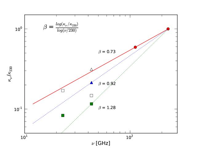
Figure 7: Mass absorption coefficients ($\kappa_{\nu}$) to produce the measured fluxes at lower frequencies with our disk model. The slopes present dust opacity spectral indexes ($\beta$) determined between a frequency and $\nu=230$ GHz. The circles mark our results, the triangles are of Wilner et al. (1996), and the squares are of Rodmann et al. (2006). The open and filled symbols present the mass absorption coefficients when free-free emission components are included and excluded, respectively. Wilner et al. (1996) estimated 30% of their flux $10\pm 1.4$ mJy at $\lambda=7$ mm for free-free emission and Rodmann et al. (2006) argued 20% of their flux 4.92 mJy at $\lambda=7$ mm and 50% of 1.63 mJy at $\lambda=1.3$ cm for free-free emission.

On the other hand, Rodmann et al. (2006) derived $\beta$=1.3 in the wavelength range of 1 to 7 mm. Extension of our $\beta$=0.73 law to 7 mm clearly overestimates the measured flux: 9.4 mJy from our model versus 3.9 mJy of disk emission estimated by Rodmann et al. (2006). To produce the measured 7 mm flux our model needs $\beta=1.28$ between $\lambda=1.3$ mm and 7 mm. Note that the model with this $\beta$ produces the same $\lambda=1.3$ mm image but it does not fit our $\lambda=2.7$ mm flux and image. Figure 7 shows the ratio of the mass absorption coefficient ($\kappa_{\nu}$) at a wavelength divided by the mass absorption coefficient at $\lambda=1.3$ mm. A straight line in this log-log plot represents a single power law index over the full wavelength range. The turnover in the ratio value could indicate a largest grain size of several millimeter in the disk (Draine, 2006).

The disk mass is very well determined within the context of the model: 0.135 M_⊙. However, the full uncertainty must include uncertainty in the absolute flux calibration, the mass absorption coefficient, the gas-to-dust ratio, and the dust temperature. We have estimated the flux calibration uncertainty at 10% which translates directly to a mass uncertainty. The mass opacity coefficient could be uncertain at the factor of two level. The total luminosity of the HL Tau system is also uncertain: estimates range from 1 to 11 L_⊙. The resulting uncertainty in the dust temperature at a fiducial radius is about 67%. Note that the massive disks constrained in thinner disk models (Figure 2) would have larger uncertainty in the gas-to-dust ratio, as the models imply grain settlement. Although the mass is uncertain, we argue that this particular model of $b_{height}=1.5$ would have the least overestimated disk mass and the least uncertainty in our modeling at about a factor of two.

The inner radius is constrained by our data to be significantly smaller than our $\lambda=1.3$ mm linear resolution of about 20 AU. The formal model fit gives an inner radius of 2.4 AU. Fits to the mid-infrared emission typically require disk material to an inner radius of several stellar radii to 0.2 AU (Men’shchikov et al., 1999; Furlan et al., 2008). It is possible that an inner radius in millimeter emission is tracing a surface density drop, but the material remains optically thick at mid-infrared wavelengths throughout the inner disk.

The characteristic radius, which divides the regions dominant by the power-law and the exponential density distributions, is 79 AU. It is this exponential cutoff in Equation (1) that sets the outer scale for the disk in the presence of the shallow power-law index. The surface density falls by a factor of ten from its peak at a distance of 125 AU, and a factor of one-hundred at 165 AU. In the context of the accretion disk model, the transitional radius $R_{t}$, the radius where the bulk flow direction changes from inward to outward for angular momentum conservation, is then 40.3 AU: $R_{t}=R_{c}(\delta/2)^{\delta},\textrm{ where }\delta=1/(2-\gamma)$ (Andrews et al., 2009). A previous study reported that $R_{t}$ gets larger with age (Isella et al., 2009) but another circumstellar disk survey did not find such a trend (Andrews et al., 2009).

The disk inclination and position angle are very well determined by the disk model: inclination of about $40\arcdeg$ (face-on disk $\theta_{i}=0\arcdeg$) and position angle of about $136\arcdeg$. In fact, these are not varying much even over the wide range of $b_{height}$ (Figure 2). The inclination is particularly consistent with previous studies using submillimeter and millimeter wavelength observations of a high angular resolution. Mundy et al. (1996) suggested a relatively wide range of $20\arcdeg$–$55\arcdeg$ and Lay et al. (1997) constrained as $42\arcdeg\pm 5\arcdeg$. Men’shchikov et al. (1999) also reported an inclination of $47\arcdeg$ using a detailed SED modeling. However, fits at infrared wavelengths have suggested inclinations from i $=15\arcdeg$ from mid-infrared spectral fits (Furlan et al., 2008), to 66–71$\arcdeg$ from fitting to near-infrared images and polarization (Lucas et al., 2004). It is possible that the near- and mid-infrared determinations of inclination are affected by large scale inhomogeneities such as the wall structure.

4.3 Constraints on the Presence of the Proposed Protoplanet and Disk Stability

Figure 8 presents the zoomed-in residual map overlaid on top of the image at $\lambda=1.3$ mm. Particularly the top-left panel displays a blow-up of the $\lambda=1.3$ mm image of the disk in the region of the protoplanet candidate (Greaves et al., 2008). The right panel shows the residuals for the same region when the disk model is removed. The cross-hashed circles of both panels mark the position where Greaves et al. (2008) claimed a protoplanet candidate. Greaves et al. (2008) detected a clump of $78\pm 17~{}\mu$Jy at $\lambda=1.3$ cm. The clump would be $25\pm 5$ mJy at $\lambda=1.3$ mm, assuming a $\nu^{2.5}$ emission spectrum. If the dust grains responsible for the emission were very large so that the emission spectrum rather followed $\nu^{2.0}$, i.e., the hardest to detect for our observations, then the flux at $\lambda=1.3$ mm would be $7.8\pm 1.7$ mJy. Since our observational sensitivity at $\lambda=1.3$ mm is 0.8 mJy beam^-1, the candidate could be detected in our observations in spite of our relatively worse angular resolution: $0.08\arcsec$ versus $0.13\arcsec$.

As shown in the panels, the candidate position is within the dust thermal emission region of the disk at $\lambda=1.3$ mm; however, subtraction of the axi-symmetric disk model removes essentially all flux. Before model subtraction the flux at the position is $\sim$16 mJy beam^-1; after subtraction the position has a negative flux at a level of 2$\sigma$. Therefore, our $\lambda=1.3$ mm image provides no support for the candidate protoplanetary condensation. The flux level before subtraction is roughly consistent with the value bootstrapped from the $\lambda=1.3$ cm flux, but it is part of the large disk structure, which was not detected by their observations, rather than a compact signal.

Although our observations do not have the protoplanet candidate signal, the HL Tau disk could be gravitationally unstable. Our disk model provides a surface density profile that can be used to calculate local gravitational stability in the disk. The Toomre Q parameter (Toomre, 1964) with values smaller than 1.5 is a good indicator for gravitationally unstable regions. The Q parameter versus radius, Figure 9, was calculated with the disk temperature and density distributions of our modeling. It shows a minimum less than or close to 1.5 in the range of 50 to 100 AU, which means that substructures can develop at these radii by gravitational instability. This result is in agreement with the work by Nero & Bjorkman (2009), which studied the possibility of fragmentation in the HL Tau disk based on perturbation cooling time and gravitational instability. Considering the surface density, protostellar mass, and the radius of our modeling in the Nero & Bjorkman (2009) results, roughly 2 $M_{Jupiter}$ fragments are favored between 50 and 100 AU. As discussed in Section 4.2, the disk mass that is the most important property for the Q parameter calculation has a large uncertainty. However, since the model used here is not even the one with a small $b_{height}$ favoring a massive disk, the HL Tau disk is likely unstable in the outer region.

Although we have not detected a clear substructure, the HL Tau disk is likely unstable and can be fragmented. The positive residual at $\sim$100 AU in Figure 8 might be a hint of a dust lane. Indeed, extrasolar planetary systems with planets at outer disk regions have been found (e.g., Kalas et al., 2008; Marois et al., 2008). These planets of outer disk regions are thought to have formed by gravitational instability (so-called the disk instability scenario), although it is little known whether and how the protoplanets formed by gravitational instability at the early phase of protoplanetary disks still having gas can survive the following active migration stage (e.g., D’Angelo et al., 2010). In contrast, the other major model of giant planet formation, so-called the core accretion scenario, cannot currently explain the giant planets at the outer disk regions due to too-large time scales of gas accretion (e.g., D’Angelo et al., 2010). Regardless of giant planets being actually formed by disk instability or core accretion, they should be formed in protoplanetary disks that still have gas. In the near future, ALMA will provide the unprecedented image to reveal the more detailed disk structure of HL Tau. In addition, we would be able to distinguish the two scenarios of giant planet formation by gas kinematics and substructure and scale height variation in multiple wavelength observations.

5 CONCLUSION

We have obtained dust continuum data of HL Tau at $\lambda=1.3$ mm and 2.7 mm with the exceptionally high image fidelity and angular resolution up to $0.13\arcsec$ using CARMA. This resolution reveals 18 AU scales at the distance of HL Tau, 140 pc. Through visibility modeling in Bayesian inference adopting the viscous accretion disk model, we constrained the physical properties of HL Tau. As we fit our two wavelength data simultaneously, we also constrained the dust opacity spectral index. In addition to the two wavelength images, we also qualitatively fit the SED.

Modeling in Bayesian inference toward the two wavelength images prefers a thin disk (Figure 2). However, thin disk models can not explain mid-infrared emission of SED (Figure 3). A thick disk is needed to produce the mid-infrared emission. The discrepancy between the fitting results of millimeter images and the SED may indicate the settlement of particularly large grains into the mid plane (a stratified settlement of dust grains). However, based on the reasonable fitting to both the millimeter images and SED and considering that dust is not the majority of disk mass, we selected and further discussed the case of $b_{height}=1.5$ (Figure 6 and Table 1), which possibly supports envelope residuals beyond the hydrostatic equilibrium thickness. The scale height ratio larger than unity might also be caused by an overestimate of the HL Tau protostellar mass or an underestimate of the disk mid-plane temperature. The $b_{height}=1.5$ model reveals that the disk mass is about 0.135 $M_{\sun}$ and the dust opacity spectral index presents that grains have grown further, compared with objects at earlier evolutionary stages. The disk inclination and position angle are well determined as $40\arcdeg$ (face-on disk of $\theta_{i}=0\arcdeg$) and $136\arcdeg$, respectively.

Although a protoplanet candidate has been claimed in HL Tau, our observations, which are more sensitive to dust thermal emission, do not detect emission structure supporting the candidate. However, HL Tau appears to be gravitationally unstable and could favor fragmentation on the Jupiter mass scale between about 50 and 100 AU. Further observations with a higher angular resolution and a higher sensitivity using ALMA will be able to show substructures possibly formed by gravitational instability as well as to verify the stratified settlement of dust grains in HL Tau.

Figure 1: HL Tau in the $\lambda=1.3$ mm continuum. The image is the combined of CARMA A, B, and C configurations, and the synthesized beam is $0\farcs 17\times 0\farcs 13$ ($PA=86\arcdeg$) corresponding to 18 AU. The contour levels are 2.5, 4.0, 6.3, 10, 16, 25, and 40 times $\sigma=\pm 0.8$ mJy beam^-1.

Figure 2: Free parameter variation along changing $b_{height}$. The thinner models are preferred by our two wavelength images, based on the posterior values. However, thin disk models cannot explain the mid-infrared fluxes (Figure 3).

Figure 3: HL Tau SED overlaid with models of various $b_{height}$ values. The solid line is the case of $b_{height}=1.5$ and the dashed lines are cases of $b_{height}=0.1$, 0.2, 0.5, 1.0, and 2.0 from the bottom. The two stars indicate our data points 700 and 120 mJy at $\lambda=1.3$ and 2.7 mm, respectively.

Figure 4: HL Tau visibility averaged in annuli. The rectangular and triangle points are data at $\lambda=1.3$ mm and 2.7 mm, respectively, and the solid line is the model best fitting to both images and SED.

Figure 5: HL Tau continuum, model, and residual maps at $\lambda=1.3$ mm and 2.7 mm. The $\lambda=1.3$ mm image is the same as Figure 1 and the synthesized beam of the $\lambda=2.7$ mm image is $0\farcs 98\times 0\farcs 70$ ($PA=80\arcdeg$). The contour levels are 2.5, 4.0, 6.3, 10, 16, 25, and 40 times $\sigma=\pm 0.8$ and $\pm 1.1$ mJy beam^-1 at $\lambda=1.3$ mm and 2.7 mm, respectively.

Figure 6: Posterior distributions of parameters in HL Tau. The solid lines of the plots indicate normal distributions of the posterior-weighted means and standard deviations of the parameter distributions. The posterior-weighted means and standard deviations are listed in Table 1 with the parameter search ranges.

Figure 8: HL Tau in the $\lambda=1.3$ mm continuum overlaid with residual contours in the bottom. The disk image is the same as Figure 1 and the levels of residual contours are 2 and 3 times $\sigma=\pm 0.8$ mJy beam^-1. The top row shows the northwest quadrant region zoomed-in. The contour levels of the left are 2.5, 3.0, 4.0, 5.0, 6.3, 8.0, 10.0, 11.5, 13.0, 14.5, 16.0, 18.0, 20.0, 22.0, 25.0, 28.0, 32.0, 36.0, and 40.0 times $\sigma=\pm 0.8$ mJy beam^-1. The red hashed circles indicate where a protoplanet has been claimed. As shown, no excess signal has been detected.

Figure 9: Toomre $Q$ parameter along radius in HL Tau. The dotted lines indicate the region when assuming factor of two uncertainty in the disk mass mainly induced by $\kappa_{0}$ uncertainty (Ossenkopf & Henning, 1994). Note that the Q value is smaller than or very close to 1.5 between 50 and 100 AU, which suggests that the region may be gravitationally unstable.

Table 1: Disk fitting results of free parameters.

Parameters		Search ranges		Fitting results	Statistical	Systematic
					Uncertainties
$p$		0.00	–3.35	1.064	0.0085	0.07
$\beta$		-0.35	–1.7	0.729	0.0069	0.25
$M_{disk}$	[M⊙]	0.005	–0.2	0.1349	0.00034	0.013
$R_{in}$	[AU]	0.1	–20	2.4	0.45	2.1
$R_{c}$	[AU]	40	–460	78.9	0.20	9
$\theta_{i}$	[$\arcdeg$]	0	–83	40.3	0.23
PA	[$\arcdeg$]	0	–180	135.8	0.35
$b_{height}$		0.05	–2.0	1.5	fixed
$\gamma$				-0.22	derived from
$R_{t}$	[AU]			40.3	fitted parameters

References

- Andrews et al. (2009) Andrews, S. M., Wilner, D. J., Hughes, A. M., Qi, C., & Dullemond, C. P. 2009, ApJ, 700, 1502
- Balsara et al. (2009) Balsara, D. S., Tilley, D. A., Rettig, T., & Brittain, S. D. 2009, MNRAS, 397, 24
- Beckwith et al. (1990) Beckwith, S. V. W., Sargent, A. I., Chini, R. S., & Guesten, R. 1990, AJ, 99, 924
- Briggs (1995) Briggs, D. S. 1995, PhD thesis, New Mexico Institute of Mining and Technology
- Carrasco-González et al. (2009) Carrasco-González, C., Rodríguez, L. F., Anglada, G., & Curiel, S. 2009, ApJ, 693, L86
- Chandler & Richer (2000) Chandler, C. J. & Richer, J. S. 2000, ApJ, 530, 851
- Corder et al. (2010) Corder, S. A., Wright, M. C. H., & Carpenter, J. M. 2010, in Society of Photo-Optical Instrumentation Engineers (SPIE) Conference Series, Vol. 7733, Society of Photo-Optical Instrumentation Engineers (SPIE) Conference Series
- D’Angelo et al. (2010) D’Angelo, G., Durisen, R. H., & Lissauer, J. J. 2010, Giant Planet Formation, ed. Seager, S., 319–346
- Draine (2006) Draine, B. T. 2006, ApJ, 636, 1114
- Dullemond & Dominik (2004a) Dullemond, C. P. & Dominik, C. 2004a, A&A, 417, 159
- Dullemond & Dominik (2004b) —. 2004b, A&A, 421, 1075
- Furlan et al. (2008) Furlan, E., McClure, M., Calvet, N., et al. 2008, ApJS, 176, 184
- Gilks et al. (1996) Gilks, W. R., Richardson, S., & Spiegelharlter, D. J. 1996, Markov Chain Monte Carlo in Practice (Chapman and Hall)
- Goldreich & Ward (1973) Goldreich, P. & Ward, W. R. 1973, ApJ, 183, 1051
- Greaves et al. (2008) Greaves, J. S., Richards, A. M. S., Rice, W. K. M., & Muxlow, T. W. B. 2008, MNRAS, 391, L74
- Isella et al. (2009) Isella, A., Carpenter, J. M., & Sargent, A. I. 2009, ApJ, 701, 260
- Kalas et al. (2008) Kalas, P., Graham, J. R., Chiang, E., et al. 2008, Science, 322, 1345
- Kitamura et al. (2002) Kitamura, Y., Momose, M., Yokogawa, S., et al. 2002, ApJ, 581, 357
- Kwon (2009) Kwon, W. 2009, PhD thesis, University of Illinois at Urbana-Champaign
- Kwon et al. (2009) Kwon, W., Looney, L. W., Mundy, L. G., Chiang, H., & Kemball, A. J. 2009, ApJ, 696, 841
- Lamb et al. (2009) Lamb, J., Woody, D., Bock, D., et al. 2009, in SPIE Newsroom
- Lay et al. (1997) Lay, O. P., Carlstrom, J. E., & Hills, R. E. 1997, ApJ, 489, 917
- Looney et al. (2000) Looney, L. W., Mundy, L. G., & Welch, W. J. 2000, ApJ, 529, 477
- Lucas et al. (2004) Lucas, P. W., Fukagawa, M., Tamura, M., et al. 2004, MNRAS, 352, 1347
- MacKay (2003) MacKay, D. J. C. 2003, Information Theory, Inference, and Learning Algorithms (Cambridge, UK: Cambridge University Press)
- Marois et al. (2008) Marois, C., Macintosh, B., Barman, et al. 2008, Science, 322, 1348
- Mathis et al. (1977) Mathis, J. S., Rumpl, W., & Nordsieck, K. H. 1977, ApJ, 217, 425
- Men’shchikov et al. (1999) Men’shchikov, A. B., Henning, T., & Fischer, O. 1999, ApJ, 519, 257
- Mundt et al. (1990) Mundt, R., Buehrke, T., Solf, J., Ray, T. P., & Raga, A. C. 1990, A&A, 232, 37
- Mundy et al. (1996) Mundy, L. G., Looney, L. W., Erickson, W., et al. 1996, ApJ, 464, L169
- Nero & Bjorkman (2009) Nero, D. & Bjorkman, J. E. 2009, ApJ, 702, L163
- Ossenkopf & Henning (1994) Ossenkopf, V. & Henning, T. 1994, A&A, 291, 943
- Pérez et al. (2010) Pérez, L. M., Lamb, J. W., Woody, D. P., et al. 2010, ApJ, 724, 493
- Pringle (1981) Pringle, J. E. 1981, ARA&A, 19, 137
- Rebull et al. (2004) Rebull, L. M., Wolff, S. C., & Strom, S. E. 2004, AJ, 127, 1029
- Robitaille et al. (2007) Robitaille, T. P., Whitney, B. A., Indebetouw, R., & Wood, K. 2007, ApJS, 169, 328
- Rodmann et al. (2006) Rodmann, J., Henning, T., Chandler, C. J., Mundy, L. G., & Wilner, D. J. 2006, A&A, 446, 211
- Sargent & Beckwith (1991) Sargent, A. I. & Beckwith, S. V. W. 1991, ApJ, 382, L31
- Sault et al. (1995) Sault, R. J., Teuben, P. J., & Wright, M. C. H. 1995, in Astronomical Society of the Pacific Conference Series, Vol. 77, Astronomical Data Analysis Software and Systems IV, ed. R. A. Shaw, H. E. Payne, & J. J. E. Hayes, 433
- Spitzer (1978) Spitzer, L. 1978, Physical processes in the interstellar medium (New York Wiley-Interscience, 1978. 333 p.)
- Thompson et al. (2001) Thompson, A. R., Moran, J. M., & Swenson, Jr., G. W. 2001, Interferometry and Synthesis in Radio Astronomy, 2nd Edition (Interferometry and synthesis in radio astronomy by A. Richard Thompson, James M. Moran, and George W. Swenson, Jr. 2nd ed. New York : Wiley, c2001.xxiii, 692 p. : ill. ; 25 cm. “A Wiley-Interscience publication.” Includes bibliographical references and indexes. ISBN : 0471254924)
- Tilley et al. (2010) Tilley, D. A., Balsara, D. S., Brittain, S. D., & Rettig, T. 2010, MNRAS, 403, 211
- Toomre (1964) Toomre, A. 1964, ApJ, 139, 1217
- Welch et al. (2000) Welch, W. J., Hartmann, L., Helfer, T., & Briceño, C. 2000, ApJ, 540, 362
- Welch et al. (2004) Welch, W. J., Webster, Z., Mundy, L., Volgenau, N., & Looney, L. 2004, in IAU Symposium, Vol. 213, Bioastronomy 2002: Life Among the Stars, ed. R. Norris & F. Stootman, 59
- Wilner et al. (1996) Wilner, D. J., Ho, P. T. P., & Rodriguez, L. F. 1996, ApJ, 470, L117
- Woody et al. (2004) Woody, D. P., Beasley, A. J., Bolatto, A. D., et al. 2004, in Presented at the Society of Photo-Optical Instrumentation Engineers (SPIE) Conference, Vol. 5498, Millimeter and Submillimeter Detectors for Astronomy II. Edited by Jonas Zmuidzinas, Wayne S. Holland and Stafford Withington Proceedings of the SPIE, Volume 5498, pp. 30-41 (2004)., ed. C. M. Bradford, P. A. R. Ade, J. E. Aguirre, J. J. Bock, M. Dragovan, L. Duband, L. Earle, J. Glenn, H. Matsuhara, B. J. Naylor, H. T. Nguyen, M. Yun, & J. Zmuidzinas, 30–41
- Zacharias et al. (2003) Zacharias, N., Urban, S. E., Zacharias, M. I., et al. 2003, VizieR Online Data Catalog, 1289, 0