LoCuSS: The Sunyaev-Zel’dovich Effect and Weak Lensing Mass Scaling Relation

Abstract

We present the first weak-lensing-based scaling relation between galaxy cluster mass, $M_{\mathrm{WL}}$, and integrated Compton parameter $Y_{\mathrm{sph}}$. Observations of 18 galaxy clusters at $z\simeq 0.2$ were obtained with the Subaru 8.2-m telescope and the Sunyaev-Zel’dovich Array. The $M_{\mathrm{WL}}$$-$$Y_{\mathrm{sph}}$ scaling relations, measured at $\Delta$ = 500, 1000, and 2500 $\rho_{c}$, are consistent in slope and normalization with previous results derived under the assumption of hydrostatic equilibrium (HSE). We find an intrinsic scatter in $M_{\mathrm{WL}}$ at fixed $Y_{\mathrm{sph}}$ of 20%, larger than both previous measurements of $M_{\mathrm{HSE}}-\mbox{$Y_{\mathrm{sph}}$}$ scatter as well as the scatter in true mass at fixed $Y_{\mathrm{sph}}$ found in simulations. Moreover, the scatter in our lensing-based scaling relations is morphology dependent, with 30 – 40% larger $M_{\mathrm{WL}}$ for undisturbed compared to disturbed clusters at the same $Y_{\mathrm{sph}}$ at $r_{\mbox{\scriptsize 500}}$. Further examination suggests that the segregation may be explained by the inability of our spherical lens models to faithfully describe the three-dimensional structure of the clusters, in particular, the structure along the line-of-sight. We find that the ellipticity of the brightest cluster galaxy, a proxy for halo orientation, correlates well with the offset in mass from the mean scaling relation, which supports this picture. This provides empirical evidence that line-of-sight projection effects are an important systematic uncertainty in lensing-based scaling relations.

1. Introduction

Galaxy clusters are tracers of the highest peaks in the matter density field, and as such, their abundance as a function of mass and redshift depends strongly upon cosmology. Along with data from a variety of other techniques (Komatsu et al., 2011; Hicken et al., 2009; Kessler et al., 2009; Percival et al., 2010), galaxy cluster surveys have placed precise constraints on the $\Lambda$CDM cosmological parameters (Vikhlinin et al., 2009b; Mantz et al., 2010b). To improve the constraints from cluster surveys, the scaling relationship between survey observables and the total cluster mass must be precisely determined.

Surveys at millimeter wavelengths can be used to identify large numbers of clusters via the Sunyaev-Zel’dovich (SZ) effect, as has been demonstrated by the South Pole Telescope (SPT; Staniszewski et al. 2009; Vanderlinde et al. 2010; Williamson et al. 2011), the Atacama Cosmology Telescope (ACT; Marriage et al. 2011), and the Planck satellite (Planck Collaboration et al., 2011). The SZ effect is a spectral distortion of the cosmic microwave background (CMB) resulting from the inverse Compton scattering of CMB photons by the hot electrons of the intra-cluster medium (ICM). The magnitude of this distortion is determined by the integral of the pressure along the line of sight through the cluster. The volume integral of pressure is the total thermal energy content of the ICM, which should directly trace the depth of the potential well (Carlstrom et al., 2002), so a tight scaling between the SZ signal ($Y$, see Section 3.2) and mass is expected.

A low-scatter correlation is indeed found in simulations of galaxy clusters (e.g., da Silva et al., 2004; Motl et al., 2005; Nagai, 2006; Stanek et al., 2010), and is suggested in the best comparisons of SZ observations and cluster mass estimates available to date (Bonamente et al., 2008; Plagge et al., 2010; Andersson et al., 2011). However, the mass-$Y$ scaling relation remains poorly determined from these observations, and the uncertainty in the relation is already limiting the cosmological constraints derived from small SZ-selected samples (Vanderlinde et al., 2010; Sehgal et al., 2011). Moreover, previous comparisons of $Y$ with mass have relied on mass estimates derived assuming hydrostatic equilibrium (HSE). This assumption is certain to result in at least some bias, although the degree of bias is poorly known; observational constraints suggest $\lesssim 20$% within radii of interest (Mahdavi et al., 2008; Zhang et al., 2010), though some simulations have found larger biases (e.g., Cavaliere et al., 2011).

One promising technique for improving our knowledge of the mass-$Y$ relation is weak gravitational lensing (e.g., Dahle et al., 2002; Hoekstra, 2007; Okabe et al., 2010a). Unlike other techniques, weak lensing directly probes the gravitational potential of the cluster, providing a way to test for mass biases in other mass estimators. However, the weak lensing signal is sensitive to the total mass projected along the line-of-sight, and thus likely suffers projection-related errors in mass measurements (e.g., Metzler et al., 2001; Hoekstra, 2001, 2003). Several authors have calibrated X-ray observables against lensing mass estimates, typically finding consistency with (but with larger scatter than) X-ray-only scaling relations (Smith et al., 2005; Bardeau et al., 2007; Hoekstra, 2007; Zhang et al., 2007, 2008; Rykoff et al., 2008; Okabe et al., 2010b; Hoekstra et al., 2011). This technique has not yet been used to calibrate the SZ observable except in the cluster core (Marrone et al., 2009). An important next step is to make such a comparison at the larger radii typically used in cosmological studies with galaxy clusters.

The calibration of mass-observable relations is one of the key goals of the Local Cluster Substructure Survey (LoCuSS), a multi-wavelength survey of galaxy clusters at $0.15<z<0.3$ selected from the ROSAT All-sky Survey (Ebeling et al., 1998, 2000; Böhringer et al., 2004). The large luminosity range and lack of morphological selection in the sample ensure a morphologically diverse population for calibration studies. Weak lensing mass estimates are available for an initial sample of 29 LoCuSS clusters (Okabe et al. 2010a; hereafter Ok10). In this paper, we combine these estimates with SZ data from the Sunyaev-Zel’dovich Array (SZA) in order to examine the mass-$Y$ scaling relation and its scatter. We also explore the possibility of biases in the mass estimates related to cluster morphology, which our data suggest is an important systematic.

Section 2 describes the sample of clusters as well as the weak lensing and SZ observations. In Section 3, we discuss the analysis techniques used to derive the weak lensing mass estimates and determine the SZ observables. Our scaling relation results are presented in Section 4 and our interpretation of the findings is discussed in Section 5. Our conclusions are reviewed in Section 6. We assume a flat $\Lambda$CDM cosmology: $\Omega_{\mathrm{M}}=0.27$, $\Omega_{\Lambda}=0.73$, $H_{0}=73\rm~{}km~{}s^{-1}~{}Mpc^{-1}$.

2. Observations

2.1. Cluster Sample

The clusters considered in this work are drawn from the LoCuSS “high-$L_{\rm X}$” sample discussed by Ok10 (G. P. Smith, in prep.), which was selected from the ROSAT All-Sky Survey to have $0.15<z<0.3$, $-20^{\circ}\leq\delta\leq+60^{\circ}$, and $n_{H}<7\times 10^{20}{\rm cm}^{-2}$. This sample is subject to a luminosity limit of $L_{\mathrm{X}}/E(z)^{2.7}>4.1\times 10^{44}$ ergs, where $E(z)$ describes the redshift evolution of the Hubble parameter ($E(z)^{2}\equiv H(z)^{2}/H_{0}^{2}=\Omega_{M}(1+z)^{3}+\Omega_{\Lambda}$ for a flat cosmology). Specifically, we consider 21 clusters from the high-$L_{\rm X}$ sample (Table 1) for which high quality $V$- and $i^{\prime}$-band Subaru/Suprime-Cam data are available, and in which a central mass concentration is identifiable in the shear maps (see Table 5 of Ok10, ). The sample spans a factor of $4$ in X-ray luminosity and includes clusters with a broad range of X-ray morphologies, including cool-core (hereafter CC) clusters (e.g., A 383, A 1835: Smith et al., 2001; Schmidt et al., 2001), cold front clusters (e.g., RX J1720.1$+$2638: Mazzotta et al., 2001), and clusters known to be undergoing mergers (e.g., A 209: Giovannini et al., 2009, and references therein).

2.2. Gravitational Lensing

The acquisition and processing of the Subaru/Suprime-Cam data upon which the weak lensing mass measurements are based are described in detail by Ok10. Briefly, the data were acquired in the $V$- and $i^{\prime}$-bands in excellent atmospheric conditions ${\rm FWHM}\simeq 0.7^{\prime\prime}$, consistent with the stringent requirements for precise measurement of galaxy shapes. Weakly-lensed background galaxies were selected to have a minimum color offset from the cluster red sequence in the color-magnitude plane following Umetsu & Broadhurst (2008) and Umetsu et al. (2009). Background galaxy shapes were measured using KSB (Kaiser et al., 1995), achieving a residual mean ellipticity of point sources after removal of the point spread function of $\sim 10^{-4}$, and a typical number density of galaxies for use in the weak lensing analysis of $\sim 10-30$ arcmin^-2.

2.3. Sunyaev-Zel’dovich Effect

The sample of 21 clusters was observed with the SZA, an 8-element radio interferometer optimized for measurements of the SZ effect. The SZA is a subset of the 23-element Combined Array for Research in Millimeter-wave Astronomy (CARMA). Data were obtained in an 8 GHz passband centered at 31 GHz between 2006 and 2009 (Table 1). Over the period of these observations, the array was sited at two different locations and occupied three different configurations, as described in Culverhouse et al. (2010). For most of this period, the SZA was configured with six elements in a compact array sensitive to arcminute-scale SZ signals, and two outrigger elements providing discrimination for compact radio source emission. The compact array and outrigger baselines provide baseline lengths, in units of number of wavelengths $\lambda$, of 0.35$-$1.3 k$\lambda$ and 2$-$7.5 k$\lambda$, respectively. Two of the clusters (Abell 209 and ZwCl 1454.8+2233) were also briefly observed with an eight-compact-element array configuration, with greater SZ sensitivity but little intrinsic power to distinguish SZ signal from contamination. Integration times were tailored to the magnitude of the SZ signal in each cluster and, secondarily, to the degree of contamination from radio sources. Clusters with complex radio source environments in 1.4 GHz survey images were given more integration time. The total on-source unflagged integration times range from 5 to 69 hours, and the corresponding noise levels achieved by the short (SZ-sensitive) baselines were 0.14 to 0.45 mJy (12 to 40 $\mu$K), with synthesized beams of $\sim$2′ FWHM. Absolute calibration of the data is determined through periodic measurements of Mars, calibrated against the Rudy et al. (1987) model for this source. A systematic uncertainty of 10% applies to the SZ measurements due to the uncertainty in the absolute calibration (Sharp et al., 2010), this is not included in the reported errors.

Exclusion of emissive sources from the SZA data is most simply achieved when the sources are spatially compact. For such sources the emission measured on the longer outrigger baselines (smaller angular scales) can be assumed to be representative of the emission measured on the short, SZ-sensitive baselines (larger angular scales) and thereby separated from the SZ signal. Sources that are not point-like on the scale of 20″ leave residual emission in the short baseline maps that fills in the cluster SZ signal. Three clusters in the sample suffer from extended radio source contamination:

• Abell 115 hosts the bright radio source 3C 28, which is $>$100 mJy at 5 GHz and has lobes extending more than an arcminute across the cluster (Giovannini et al., 1987). While there is some discrimination on the short baselines between the extended central source and the more extended SZ decrement, reliable separation of these two resolved structures is not possible in these data.

• RX J1720.1+2638 contains a bright source near the cluster center that is resolved on scales of 30″ at 1.4 GHz in the VLA FIRST survey (Becker et al., 1995). The SZA data suggest that this source is also extended at 31 GHz, where the SZ decrement appears to be split through its center by an emissive source after a point-like source model is determined from the long baselines and removed.

• Abell 291 hosts three 31 GHz sources within an arcminute of the pointing center. One of these is revealed to be a double-lobed radio source in FIRST, and residual emission at this position appears to fill in the SZ decrement, leading to an offset of $>$20″ between the SZ centroid and BCG position.

Observations of these objects in the 90 GHz SZA band would likely provide greater spectral discrimination between the radio source emission and SZ signal; this possibility will be examined through future observations.

In subsequent sections we analyze the sample of 18 clusters that remains after excluding the three objects described above. As in Ok10, we examine whether the 18-cluster subsample is representative of the parent sample by constructing randomized (with replacement) groups of the same size from the full sample. We find that the mean value of $L_{\mathrm{X}}/E(z)^{2.7}$ for our sample is very similar to the parent population, falling in the 47^th percentile of random groups. The spread in $L_{\mathrm{X}}/E(z)^{2.7}$ within the sample is also very representative, the standard deviation in this quantity for our sample is again at the 47^th percentile of the random groups.

Table 1Cluster Sample and SZ Observational Parameters

Cluster	R.A.	Dec	$z$	$L_{\mathrm{X}}[0.1-2.4\mathrm{keV}]$	$t_{int}$	$S_{rms}$	Resolution	$T_{rms}$
				($10^{44}\mbox{${\rm erg\,s^{-1}}$}$)	(hrs)	(mJy)	(″)	($\mu$K)
Abell 68	00:37:05.90	$+$09:09:26.6	0.255	8.8	17.3	0.22	122$\times$139	17
Abell 115N	00:55:50.38	$+$26:24:36.0	0.197	8.6	7.7	0.36	126$\times$130	29
Abell 209	01:31:53.47	$-$13:36:46.1	0.206	7.3	19.3	0.21	91$\times$125	24
RX J0142.0$+$2131	01:42:02.64	$+$21:31:19.2	0.280	5.9	11.6	0.30	114$\times$126	27
Abell 267	01:52:41.93	$+$01:00:24.1	0.230	8.1	18.4	0.30	115$\times$160	21
Abell 291	02:01:43.11	$-$02:11:48.1	0.196	5.7	27.8	0.22	101$\times$124	23
Abell 383	02:48:03.50	$-$03:31:45.0	0.188	5.3	25.0	0.27	128$\times$159	18
Abell 521	04:54:06.90	$-$10:13:24.6	0.247	9.5	12.8	0.32	117$\times$210	26
Abell 586	07:32:20.31	$+$31:38:02.0	0.171	6.6	13.1	0.25	120$\times$137	21
Abell 611	08:00:56.74	$+$36:03:21.6	0.288	8.1	30.2	0.25	120$\times$130	21
Abell 697	08:42:57.80	$+$36:21:54.5	0.282	9.6	15.8	0.35	118$\times$128	30
Abell 1835	14:01:02.02	$+$02:52:41.7	0.253	22.8	13.5	0.36	117$\times$149	27
ZwCl 1454.8+2233	14:57:15.09	$+$22:20:34.2	0.258	7.8	68.6	0.14	119$\times$123	12
ZwCl 1459.4+4240	15:01:23.13	$+$42:20:39.6	0.290	6.7	21.7	0.22	115$\times$131	19
Abell 2219	16:40:22.60	$+$46:42:22.0	0.228	12.1	27.3	0.20	114$\times$133	17
RX J1720.1+2638	17:20:09.90	$+$26:37:27.8	0.164	9.5	26.9	0.19	108$\times$125	19
Abell 2261	17:22:27.08	$+$32:07:58.6	0.224	10.8	9.9	0.31	114$\times$134	26
RX J2129.6+0005	21:29:39.90	$+$00:05:19.8	0.235	11.0	24.5	0.27	113$\times$167	19
Abell 2390	21:53:36.70	$+$17:41:31.0	0.233	12.7	4.8	0.45	109$\times$136	40
Abell 2485	22:48:31.13	$-$16:06:25.6	0.247	5.9	21.2	0.19	106$\times$126	18
Abell 2631	23:37:38.80	$+$00:16:06.5	0.278	7.9	16.1	0.28	140$\times$152	17

3. Analysis

3.1. Weak Gravitational Lensing

The procedures for determining galaxy cluster masses and related radii are described in full by Ok10; we summarize salient details here. We adopt Ok10’s “red+blue” galaxy sample – i.e., we use only those galaxies that are redder or bluer than the cluster red sequence. Exclusion of unlensed galaxies in this manner is essential because cluster/foreground galaxies can bias $M_{\mbox{\scriptsize 2500}}$ and $M_{\mbox{\scriptsize 500}}$ low by $\sim 50-20\%$. The mean redshift of the color-selected background galaxies is estimated by matching their colors and magnitudes to the COSMOS photometric redshift catalog (Ilbert et al., 2009). The tangential shear signal is then measured in logarithmically spaced bins, the measurement in each bin being the error-weighted mean tangential shear of the galaxies in that bin. The bins are centered on the brightest cluster galaxy (BCG) of each cluster.

The spherical mass (or spherical overdensity mass) $M_{\Delta}$ is defined as the mass enclosed within a radius $r_{\Delta}$ for which the average interior density is $\Delta$ times the critical density of the universe ($\rho_{c}\equiv 3H(z)^{2}/8\pi G$). $M_{\Delta}$ is estimated by fitting the measured shear profile to the NFW model prediction parameterized by $M_{\Delta}$ and concentration $c_{\Delta}$, where the NFW mass profile (Navarro et al., 1996) is given as $\rho\propto r^{-1}(1+c_{\Delta}r/r_{\Delta})^{-2}$. Both $M_{\Delta}$ and $c_{\Delta}$ are allowed to be free in the fit—no mass-concentration relation is assumed, as is often done in other works (e.g., Hoekstra, 2007)—and the $M_{\Delta}$ values for each cluster are determined by marginalizing over the posterior distribution of concentration values. Spherical weak lensing masses at two of the three overdensities used in this work, $\Delta=$ 2500 and 500, are listed in Table 8 of Ok10. Values for $\Delta=1000$ are calculated from the mass profiles fitted in that work. Overdensity radii, which are calculable from the masses ($M_{\Delta}=4\pi r_{\Delta}^{3}\Delta\rho_{c}/3$), are given in Table 4.

3.2. Integrated Sunyaev-Zel’dovich Effect Signal

For scaling relation analyses, the SZ signal is typically quantified using the Compton $y$-parameter integrated within a region centered on a cluster:

$$Y = \int yd\Omega=\frac{1}{D_{\mathrm{A}}^{2}}\frac{k_{B}\sigma_{T}}{m_{\mathrm{e}}c^{2}}\int dl\int n_{\mathrm{e}}T_{\mathrm{e}}dA$$ (1)

$$= \frac{1}{D_{\mathrm{A}}^{2}}\frac{\sigma_{T}}{m_{\mathrm{e}}c^{2}}\int dl\int P(r)dA.$$

The quantity $YD_{\mathrm{A}}^{2}$ is called the intrinsic $y$-parameter, as it removes the distance dependence of the right side of Equation 1.

It is customary to integrate Compton-$y$ over the solid angle subtended by the cluster, as the average change in the CMB temperature within an aperture ($\overline{\Delta T}\propto YT_{\mathrm{CMB}}$) is expected to be a robust observable. One standard method of accomplishing this is to compare the observed sky signal with a parameterized radial SZ profile, projected to two dimensions and filtered in the same way as the sky data. However, both in interferometric data such as ours and in data from single-aperture telescopes, the large-scale SZ signal is attenuated by spatial filtering and/or confused with the anisotropy of the primary CMB (e.g., Plagge et al., 2010). The poor constraint on the large-scale behavior of the profile is coupled into the derived $Y$ as additional uncertainty from the unknown large $l$ (line of sight distance) behavior of the profile.

This effect can be partially mitigated by adopting as an observable the integral of the model profile over a spherical volume,

$$Y_{\mathrm{sph}}=\frac{1}{D_{\mathrm{A}}^{2}}\frac{\sigma_{T}}{m_{\mathrm{e}}c^{2}}\int P(r)dV.$$ (2)

$Y_{\mathrm{sph}}$ is relatively insensitive to the unconstrained modes in the data, and can be calculated without resorting to arbitrary outer radius cutoffs for the line-of-sight integration (as noted by Arnaud et al., 2010). Furthermore, such integration is standard in the analysis of X-ray measurements of clusters (e.g., Zhang et al., 2008; Vikhlinin et al., 2009a). We therefore perform our scaling relation analysis using the spherically integrated intrinsic $y$-parameter, $Y_{\mathrm{sph}}D_{\mathrm{A}}^{2}$.

Since interferometers do not measure the total sky signal, but instead sample the Fourier transform of the sky signal only at the spatial frequencies determined by their $uv$ coverage, we must restore missing spatial information in order to determine our observable. We accomplish this by adopting a model profile to fit to our visibility data; specifically, the generalized NFW (GNFW) pressure profile proposed by Nagai et al. (2007),

$$P(r)=\frac{P_{0}}{x^{\gamma}\left(1+x^{\alpha}\right)^{(\beta-\gamma)/\alpha}},$$ (3)

where $x\equiv r/r_{\mathrm{s}}$. The model contains five parameters: three exponents ($\alpha$, $\beta$, $\gamma$) which determine the shape of the profile, a normalization $P_{0}$, and a scale radius $r_{\mathrm{s}}$ (alternatively, a concentration parameter).

Our data are not capable of placing useful constraints on the three shape parameters due to degeneracies between them, the moderate signal to noise, and the limited range of angular scales probed by the interferometer. We fix the values of the shape parameters to the Arnaud et al. (2010) average values, [$\alpha$, $\beta$, $\gamma$]=[1.05, 5.49, 0.31], which were determined from simulations and scaled X-ray pressure profiles of galaxy clusters in the low-redshift ($z<0.2$) REXCESS sample. We consider other observationally motivated values of $\alpha$, $\beta$, and $\gamma$ (derived from morphological subsamples in Arnaud et al. 2010, see also section 5.4) to determine the range of systematic error that may be introduced by the fixed profile shape. The systematic uncertainty in $Y$ is found to range from 1 to 9% between $r_{\mbox{\scriptsize 2500}}$ and $r_{\mbox{\scriptsize 500}}$ in our data.

We estimate the remaining pressure model parameters ($P_{0}$, $r_{s}$, and the centroid position) and their uncertainties using a Markov chain Monte Carlo method (MCMC; Bonamente et al. 2006). At each step of the MCMC, we integrate the spherical profile along the line of sight, filter it with the primary beam pattern of the SZA antennas (approximately a gaussian with FWHM 11.0′), and Fourier transform for comparison with the measured Fourier components (visibilities). The positions and fluxes of detected radio sources are included in the MCMC as additional free parameters, and are marginalized over to determine the pressure model parameters.

The centroid of the SZ signal is a free parameter in our model to allow for the possibility of real offsets between the center of the ICM and the BCG. The typical uncertainty in the best-fit SZ centroid is 0.03$r_{\mbox{\scriptsize 500}}$, corresponding to $\sim$10″. For all 18 clusters, the best-fit SZ centroid is within 0.15$r_{\mbox{\scriptsize 500}}$ of the BCG position (the assumed center of shear), with the SZ centroid in $75\%$ of our sample lying within $0.04\mbox{$r_{\mbox{\scriptsize 500}}$}$ of the respective BCGs. Larger offsets were typically found in clusters that lack a cool core, or show signs of merger activity. For example, the most significant offset is seen in A 2390 ($r_{\mathrm{SZ-WL}}=0.15\pm 0.04$$r_{\mbox{\scriptsize 500}}$), which shows both a cool core and merger activity (Allen et al., 2001). After accounting for the measurement uncertainty, the distribution of offsets is reasonably consistent with recent X-ray/optical studies (Sanderson et al., 2009; Haarsma et al., 2010).

To calculate $Y_{\mathrm{sph}}$ for each cluster, we integrate the respective ICM model (Equations 2 & 3) over the spherical volume defined by the overdensity radii obtained from the weak lensing models (Section 3.1; Table 4). These radii are not constrained from the SZ data alone, so a completely independent determination of $Y_{\mathrm{sph}}$ at the overdensities of interest is not possible. The correlation between $M_{\mathrm{WL}}$ and $Y_{\mathrm{sph}}$ introduced by this procedure is discussed in Section 5.2. Note that the shared value of $r_{\Delta}$ is the only coupling between the measurements of $Y_{\mathrm{sph}}$ and the lensing analysis—there is no joint fitting of the mass and pressure profiles. The final $Y_{\mathrm{sph}}$ measurements are listed in Table 4. Because of parameter correlations, chiefly between $P_{0}$ and $r_{\mathrm{s}}$, we do not report best-fit values of the individual profile parameters for each cluster. However, as shown in Section 4.4 of Mroczkowski et al. (2009), the value of $Y_{\mathrm{sph}}$ determined from the $P_{0}$$-$$r_{\mathrm{s}}$ pairs in the Markov chain is better constrained than either of these two parameters alone.

3.3. Morphological Classification

One of our aims is to check whether the shape, normalization, and intrinsic scatter of the mass-$Y_{\mathrm{sph}}$ relation depends on cluster properties. Of particular interest is whether clusters might exhibit different behavior based on their dynamical state, which we often classify simply as merging or non-merging; however, dynamical state is difficult to estimate from SZ and weak lensing measurements alone. Here we employ a simple and broadly-accepted indicator of dynamical state: the centroid shift parameter $\left<w\right>$, defined as the standard deviation of the projected separation between the X-ray peak and the centroid of emission calculated in circular apertures centered on the X-ray peak.

We measure $\left<w\right>$ for each cluster in our sample using archival Chandra data, following the method of Mohr et al. (1995) as implemented by Maughan et al. (2008). The analysis is performed on exposure-corrected images with sources masked. The core ($<30{\rm~{}kpc}$) is excised from the calculation of the centroid, and the radii span 0.05$r_{\mbox{\scriptsize 500}}$ to $r_{\mbox{\scriptsize 500}}$ in steps of 5% of $r_{\mbox{\scriptsize 500}}$. The core is included in the calculation of the X-ray peak. The error on $\left<w\right>$ is derived from the standard deviation observed in cluster images resimulated with Poisson noise, following Böhringer et al. (2010). Previous observational studies of the $\left<w\right>$ distribution (e.g., Maughan et al., 2008; Pratt et al., 2009; Böhringer et al., 2010) have often divided clusters into “disturbed” and “undisturbed” sub-samples at $\mbox{$\left<w\right>$}=10^{-2}\mbox{$r_{\mbox{\scriptsize 500}}$}$. We adopt this value to aid comparison of our results with the literature. Six of the 18 clusters are classified as disturbed ($\mbox{$\left<w\right>$}>10^{-2}\mbox{$r_{\mbox{\scriptsize 500}}$}$), and the remaining 12 as undisturbed ($\mbox{$\left<w\right>$}<10^{-2}\mbox{$r_{\mbox{\scriptsize 500}}$}$; Table 4). Note that although much of our discussion makes use of this binary morphological classification system, equating the disturbed systems with mergers and undisturbed systems with non-mergers, the true relationship between centroid shift and dynamical state is likely to be more complex.

4. Results

The weak-lensing mass and $Y_{\mathrm{sph}}$ measurements are compared in Figure 1, and a positive correlation is evident at all radii. In this section, we define the scaling relation model that we will fit to the data, describe the regression analysis, and present the main results.

Table 2Cluster Mass and $Y_{\mathrm{sph}}$

Cluster	$\left<w\right>$	$r_{2500}$	$M_{2500}$	$Y_{\mathrm{sph,2500}}D_{\mathrm{A}}^{2}$	$r_{1000}$	$M_{1000}$	$Y_{\mathrm{sph,1000}}D_{\mathrm{A}}^{2}$	$r_{500}$	$M_{500}$	$Y_{\mathrm{sph,500}}D_{\mathrm{A}}^{2}$
	($10^{-2}$ $r_{500}$)	(Mpc)	($10^{14}$ M⊙)	($10^{-5}$ Mpc2)	(Mpc)	($10^{14}$ M⊙)	($10^{-5}$ Mpc2)	(Mpc)	($10^{14}$ M⊙)	($10^{-5}$ Mpc2)
Abell 68	1.17$\pm$0.14	0.41	1.37${}^{+0.57}_{-0.60}$	2.18${}^{+0.16}_{-0.15}$	0.70	2.69${}^{+0.76}_{-0.75}$	4.54${}^{+0.81}_{-0.67}$	1.01	4.01${}^{+1.18}_{-1.03}$	6.57${}^{+1.86}_{-1.39}$
Abell 209	0.68$\pm$0.10	0.48	2.11${}^{+0.44}_{-0.45}$	2.93${}^{+0.25}_{-0.23}$	0.88	5.05${}^{+0.71}_{-0.69}$	6.80${}^{+1.47}_{-1.17}$	1.32	8.49${}^{+1.26}_{-1.15}$	10.18${}^{+3.44}_{-2.39}$
RXC J0142.0+2131	0.76$\pm$0.13	0.45	1.87${}^{+0.30}_{-0.30}$	2.35${}^{+0.27}_{-0.27}$	0.72	2.95${}^{+0.52}_{-0.48}$	4.03${}^{+1.07}_{-0.88}$	0.99	3.91${}^{+0.80}_{-0.71}$	5.33${}^{+2.18}_{-1.53}$
Abell 267	1.68$\pm$0.05	0.42	1.38${}^{+0.24}_{-0.24}$	1.67${}^{+0.15}_{-0.15}$	0.67	2.31${}^{+0.41}_{-0.39}$	2.88${}^{+0.56}_{-0.50}$	0.94	3.16${}^{+0.66}_{-0.59}$	3.78${}^{+1.10}_{-0.88}$
Abell 383	0.20$\pm$0.04	0.45	1.69${}^{+0.23}_{-0.23}$	0.94${}^{+0.13}_{-0.12}$	0.70	2.53${}^{+0.41}_{-0.38}$	1.08${}^{+0.22}_{-0.19}$	0.96	3.24${}^{+0.66}_{-0.57}$	1.15${}^{+0.29}_{-0.22}$
Abell 521	5.16$\pm$0.12	0.38	1.06${}^{+0.30}_{-0.29}$	1.28${}^{+0.12}_{-0.12}$	0.67	2.37${}^{+0.46}_{-0.45}$	3.01${}^{+0.43}_{-0.39}$	0.99	3.81${}^{+0.70}_{-0.65}$	4.60${}^{+1.23}_{-0.94}$
Abell 586	0.26$\pm$0.06	0.57	3.30${}^{+0.61}_{-0.57}$	2.64${}^{+0.76}_{-0.57}$	0.89	5.02${}^{+1.21}_{-1.06}$	3.72${}^{+1.85}_{-1.14}$	1.22	6.50${}^{+1.89}_{-1.54}$	4.37${}^{+2.85}_{-1.52}$
Abell 611	0.33$\pm$0.08	0.44	1.78${}^{+0.44}_{-0.45}$	1.91${}^{+0.15}_{-0.15}$	0.75	3.39${}^{+0.60}_{-0.58}$	3.66${}^{+0.63}_{-0.56}$	1.07	4.98${}^{+0.91}_{-0.84}$	5.06${}^{+1.32}_{-1.08}$
Abell 697	0.58$\pm$0.09	0.48	2.19${}^{+0.50}_{-0.51}$	4.88${}^{+0.44}_{-0.37}$	0.85	4.96${}^{+0.74}_{-0.73}$	13.43${}^{+2.66}_{-2.10}$	1.26	8.04${}^{+1.18}_{-1.09}$	23.16${}^{+7.00}_{-5.06}$
Abell 1835	0.22$\pm$0.01	0.52	2.77${}^{+0.55}_{-0.56}$	5.92${}^{+0.30}_{-0.29}$	0.91	5.92${}^{+0.92}_{-0.87}$	10.76${}^{+1.35}_{-1.11}$	1.33	9.28${}^{+1.64}_{-1.46}$	14.05${}^{+2.59}_{-1.95}$
ZwCl 1454.8+2233	0.37$\pm$0.02	0.35	0.86${}^{+0.37}_{-0.40}$	0.77${}^{+0.08}_{-0.08}$	0.60	1.68${}^{+0.56}_{-0.52}$	1.61${}^{+0.24}_{-0.23}$	0.86	2.51${}^{+0.93}_{-0.78}$	2.34${}^{+0.48}_{-0.44}$
ZwCl 1459.4+4240	1.29$\pm$0.16	0.44	1.73${}^{+0.40}_{-0.41}$	2.48${}^{+0.20}_{-0.19}$	0.70	2.80${}^{+0.64}_{-0.59}$	5.42${}^{+0.89}_{-0.71}$	0.97	3.76${}^{+0.97}_{-0.86}$	8.50${}^{+2.11}_{-1.56}$
Abell 2219	1.75$\pm$0.03	0.58	3.63${}^{+0.57}_{-0.60}$	6.25${}^{+0.47}_{-0.45}$	0.91	5.83${}^{+0.87}_{-0.81}$	12.20${}^{+1.58}_{-1.42}$	1.27	7.77${}^{+1.44}_{-1.31}$	17.58${}^{+3.07}_{-2.61}$
Abell 2261	0.81$\pm$0.07	0.56	3.42${}^{+0.42}_{-0.43}$	2.81${}^{+0.50}_{-0.42}$	0.91	5.72${}^{+0.71}_{-0.68}$	3.84${}^{+1.23}_{-0.85}$	1.27	7.80${}^{+1.18}_{-1.08}$	4.40${}^{+1.80}_{-1.13}$
RXC J2129.6+0005	0.43$\pm$0.11	0.41	1.33${}^{+0.51}_{-0.52}$	1.82${}^{+0.13}_{-0.14}$	0.72	2.86${}^{+0.66}_{-0.68}$	4.19${}^{+0.73}_{-0.60}$	1.05	4.50${}^{+1.05}_{-0.94}$	6.39${}^{+2.01}_{-1.37}$
Abell 2390	0.78$\pm$0.03	0.54	3.03${}^{+0.43}_{-0.42}$	4.64${}^{+0.97}_{-0.83}$	0.87	5.01${}^{+0.79}_{-0.74}$	8.29${}^{+3.10}_{-2.19}$	1.21	6.81${}^{+1.24}_{-1.13}$	11.15${}^{+5.75}_{-3.55}$
Abell 2485	0.53$\pm$0.14	0.37	0.98${}^{+0.40}_{-0.41}$	1.17${}^{+0.10}_{-0.10}$	0.64	2.04${}^{+0.57}_{-0.57}$	2.48${}^{+0.37}_{-0.34}$	0.93	3.15${}^{+0.86}_{-0.76}$	3.61${}^{+0.87}_{-0.71}$
Abell 2631	1.68$\pm$0.14	0.49	2.33${}^{+0.34}_{-0.36}$	2.36${}^{+0.23}_{-0.23}$	0.76	3.58${}^{+0.48}_{-0.45}$	5.21${}^{+0.91}_{-0.78}$	1.05	4.66${}^{+0.70}_{-0.67}$

Note. — Cluster masses at $\Delta=2500$ and 500 as reported in Ok10 for NFW halo fits to the shear profile, $\Delta=1000$ derived from the profile fits used in that work. An additional systematic uncertainty of 10% in the overall scaling of the $Y$ values is not included in the errors reported here.

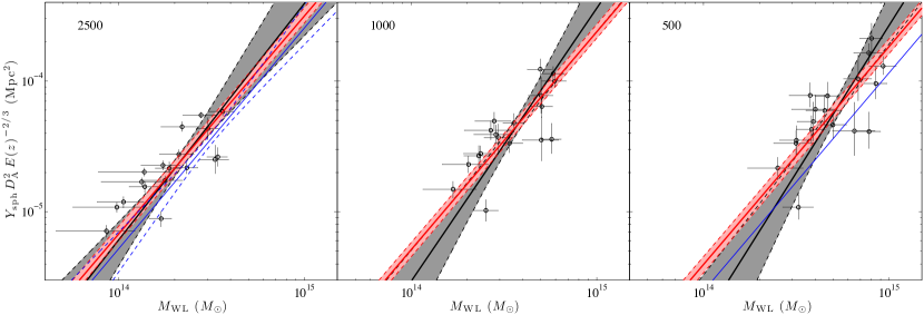
Figure 1.— The mass-$Y$ scaling relation at three overdensities, shown in the upper left corner of each plot. Two fits are shown at each overdensity: the best-fit line with a free slope is shown in black, and the best-fit line with the slope fixed to self-similar (1/$B$=5/3) is shown in red. The 1$\sigma$ uncertainty regions are shaded and marked with dashed lines. Results from prior analyses are plotted for comparison with thin blue lines: the $M$$-$$Y_{\mathrm{sph}}$ scaling relation derived from the data of Bonamente et al. (2008) (left panel), and the scaling relation from Andersson et al. (2011) (right panel).

4.1. Self-similar Scaling

Without significant influence from non-gravitational processes, the mass, temperature, size, and other properties of galaxy clusters are expected to follow self-similar scaling relations (Kaiser, 1986). These power-law relationships follow directly from the assumptions of hydrostatic equilibrium and an isothermal distribution of baryons and dark matter (e.g., Bryan & Norman, 1998), and form a useful reference point for measurements of scaling relations.

The simplest self-similar model, as derived in the above-cited papers, predicts that cluster mass ($M$) and temperature ($T$) are related as

$$T\propto M^{2/3}E(z)^{2/3}\Delta^{1/3}.$$ (4)

To derive the expected scaling between mass and the SZ signal, we note that the double integral on the right hand side of Equation 1 can be written as $M_{\mathrm{gas}}T_{\mathrm{e}}$ for an isothermal ICM, or equivalently as $f_{gas}MT_{\mathrm{e}}$ for $f_{gas}\equiv M_{gas}/M$. Combining this with Equation 4, we find the $M_{\mathrm{WL}}$$-$$Y_{\mathrm{sph}}$ scaling relation:

$$M\propto f_{gas}^{-3/5}\Delta^{-1/5}\left[YD_{\mathrm{A}}^{2}E(z)^{-2/3}\right]^{3/5}.$$ (5)

This equation defines the self-similar reference model for our scaling analysis.

4.2. Regression

We analyze the scaling between mass and $Y_{\mathrm{sph}}$ at three overdensity radii ($\Delta$ = 500, 1000, and 2500) determined from the weak lensing measurements. We fit the data with a power law of the form

$$\frac{M(r_{\Delta})}{10^{14}M_{\odot}}=10^{A}\left(\frac{Y_{\mathrm{sph}}D_{\mathrm{A}}^{2}E(z)^{-2/3}}{10^{-5}\mathrm{Mpc}^{2}}\right)^{B}.$$ (6)

The regression is performed in linearized coordinates by using the base-10 logarithm of the data points.

Our data have significant variations in their measurement precision, and simulations suggest that the $M_{\mathrm{WL}}$$-$$Y_{\mathrm{sph}}$ correlation should have intrinsic scatter, placing significant demands on our fitting technique. The problem of linear regression with uncertainty in both axes and intrinsic scatter is complex, and several methods of parameter estimation have been formulated for this circumstance (e.g., Akritas & Bershady, 1996; Tremaine et al., 2002; Weiner et al., 2006). Methods that ignore the intrinsic scatter, particularly when accompanied by heterogeneous measurement errors, lead to biased regression parameters (Kelly, 2007).

We perform our linear regression using a three-parameter model: normalization $A$, slope $B$, and intrinsic scatter $\sigma_{M|Y}$. Parameter determinations are achieved through the Bayesian regression method presented in Kelly (2007). In that work Kelly demonstrates that this method performs well in regimes where parameter estimates from other methods (OLS, BCES, FITEXY) are significantly biased. The regression is performed with publicly available IDL code written by Kelly.

4.3. Scaling Relations

Table 3$M_{\mathrm{WL}}$$-$$Y_{\mathrm{sph}}$ Scaling Relations

Note. — Scaling relations fitted according to Equation 6. For fits in the lower section of the table the power law slope was fixed to the self-similar value ($B$=3/5).

We fit the scaling relation (Equation 6) to the full sample of clusters with the slope $B$ as a free parameter, referring to the result as the “free slope” (FS) fit (Table 4.3). We also report results with the slope fixed to the self-similar value of $B=0.6$, which we refer to as the “self-similar” (SS) fit. The posterior distributions of the normalization and scatter in the SS fit are obtained by taking links with the appropriate slope from the Markov chains generated by the fitting routine.

At all three overdensity radii, the FS mass-$Y_{\mathrm{sph}}$ relations are slightly shallower than the self-similar prediction of $B=0.6$ (Figure 1), although the differences from self-similarity are not statistically significant; the relation at $\Delta=500$ is the most discrepant at $1.4\sigma$ significance. A jackknife test of the $r_{\mbox{\scriptsize 500}}$ data, dropping one cluster at a time and refitting the 17-cluster scaling relations, shows that the cluster with the lowest $Y_{\mathrm{sph,}500}$ (Abell 383) affects the slope far more than any other. Without this cluster the $r_{\mbox{\scriptsize 500}}$ scaling relation would have parameters $A=0.259^{+0.131}_{-0.138}$, $B=0.56^{+0.16}_{-0.15}$, $\sigma_{M|Y}$$=20^{+10}_{-8}$%; in this case $B$ is in no tension with the self-similar prediction. We have no strong reason to exclude this cluster, and the removal of outliers may bias the average scaling relation parameters, so no outlier clusters are excluded from the scaling relations presented in this paper.

The scaling relations reported in Table 4.3 are subject to some bias because of the $L_{\mathrm{X}}$ selection threshold of the parent LoCuSS sample. If there is a correlation between the scatter in the two ICM observables, $L_{\mathrm{X}}$ and $Y_{\mathrm{sph}}$ (or $M_{\mathrm{WL}}$), selection on the former will affect the distribution of the latter. Such correlation is not yet well-characterized observationally, however. The possibility of systematic effects in the scatter (Section 5.2), the previously noted influence of outliers in this small sample, and the possible bias from the X-ray selection demand caution when employing these scaling relations for other analyses.

The intrinsic scatter, $\sigma_{M|Y}$, is found to be $\sim 20$% at all overdensity radii, which is larger than the $\sim 10$% predicted in numerical simulations (e.g., Nagai, 2006). This holds for the SS fits as well, confirming that the measured scatter is not strongly dependent on the slope parameter.

The low scatter reported for simulated $Y$$-$$M$ scaling relations does not capture additional complications introduced by the measurement techniques. One potentially important source of scatter in our data is the contribution to $Y_{\mathrm{sph}}$ from lower mass haloes along the line of sight. This was examined by Holder et al. (2007) and found to be insignificant for our mass and redshift range. The scatter between the weak-lensing-derived mass and true halo mass may also be important. In measurements of the type used here it is expected to be $\sim 20$% (e.g., Becker & Kravtsov, 2011), which is in good agreement with the scatter we observe.

5. Discussion

5.1. Comparison to Previous Results

The $M_{\mathrm{WL}}$$-$$Y_{\mathrm{sph}}$ scaling relations presented above are the first to combine SZ measurements with weak gravitational lensing. Previous observational studies have assumed HSE to derive mass measurements, and consequently have different sets of systematics and biases. The assumption of HSE introduces an intrinsic correlation between mass and $Y_{\mathrm{sph}}$, while the intrinsic correlation between the lensing-based mass and $Y_{\mathrm{sph}}$ in our study is expected to be lower (although not necessarily zero, as discussed in §5.3). Moreover, systematic biases between HSE-based masses and lensing-based masses have been measured (Mahdavi et al., 2008) or limited at the 10% level (Zhang et al., 2008, 2010) in cluster observations, and found between HSE-based masses and true masses in simulated clusters (Rasia et al., 2006; Lau et al., 2009; Burns et al., 2010; Cavaliere et al., 2011). These simulations suggest that hydrostatic masses are biased low by $\sim 10-20\%$ at $r_{\mbox{\scriptsize 500}}$, with smaller biases at higher over-densities. In order to explore these effects, we compare our results with previous observational and theoretical studies in §5.1.1 and §5.1.2, respectively.

5.1.1 Previous Observational Results

Our results are consistent within $\sim 1\sigma$ with those of Bonamente et al. (2008) at $\Delta=2500$ (left panel of Figure 1). Bonamente et al. analysed OVRO and BIMA observations of 19 clusters at $0.14<z<0.3$ for which archival Chandra data were available. The clusters were modeled with an isothermal $\beta$-model (after excising the central 100 kpc of the X-ray data) and masses were determined assuming HSE. The $Y$ values were determined by normalizing the shape of the $\beta$-model density (or pressure, since the cluster is assumed isothermal) profile with the SZ measurements and integrating. We calculate the $Y_{\mathrm{sph}}$ values from the Markov chains used in that paper and perform the linear regression using the methods described above. Their results imply $A=0.131\pm 0.074$, $\mbox{$B$}=0.65\pm 0.12$, $\mbox{$\sigma_{M|Y}$}=9^{+7}_{-5}\%$, which are consistent with self-similarity, and are statistically indistinguishable from our best fit parameters (Table 4.3). Despite the lack of statistical significance, it is interesting to note that the intrinsic scatter in Bonamente et al.’s HSE-based scaling relation is roughly half that found in our lensing-based relation.

Our results at $\Delta=500$ agree less well with Andersson et al. (2011) (right panel of Figure 1), who examined the $\mbox{$M_{\mbox{\scriptsize 500}}$}-\mbox{$Y_{\mathrm{sph}}$}$ scaling relation for a sample of galaxy clusters discovered by the SPT (Vanderlinde et al., 2010). The mass range of the Andersson et al. (2011) sample is similar to that presented here, though at higher redshift (median $z=0.74$). They estimated cluster masses from the pressure-like X-ray observable $Y_{X}$ through an observational calibration of the $\mbox{$M_{\mbox{\scriptsize 500}}$}-Y_{X}$ scaling relation, with $M_{\mbox{\scriptsize 500}}$ measured from X-ray data assuming HSE (Vikhlinin et al., 2009a). The SZ profile, largely unresolved by the SPT, was modeled using the observed X-ray density profile and a universal temperature profile (Vikhlinin et al., 2006). The resulting scaling relation ($A=0.36\pm 0.03$, $\mbox{$B$}=0.60^{+0.12}_{-0.09}$, $\mbox{$\sigma_{M|Y}$}=9\pm 5\%$, in our nomenclature) is slightly discrepant with our FS model. However, comparison with our self-similar model is more direct, as Andersson et al.’s slope matches the self-similar value. The scatter is again roughly half that observed in our data. Their normalization is $\sim 30\%$ higher in mass at fixed $Y_{\mathrm{sph}}$ than our self-similar fit, a $2.3\sigma$ difference (after accounting for the contribution of the intrinsic scatter, compare the red and blue lines on the right panel of Fig 1). This difference is not attributable to the hydrostatic mass bias discussed above (§5.1), because the assumption of HSE results in a bias in the direction opposite to the observed discrepancy. The origin of this difference remains unclear, but systematic effects in our data, discussed below, may play a significant role.

5.1.2 Previous Simulations

Accurate calibration of numerical simulations is a key step towards cosmological application of SZ surveys. Many authors have therefore developed simulations of increasing sophistication, five recent examples of which are over-plotted on our data in Figure 2. In all cases we show the predicted scaling relation between mass and $Y_{\mathrm{sph}}$, using fits provided by the authors for those simulation studies that did not publish a mass-$Y_{\mathrm{sph}}$ relation. The simulated relations are very close to self-similar ($B=0.6$; Table 4), and slightly under-predict $Y_{\mathrm{sph}}$ at fixed mass relative to our best-fit self-similar model (red line in Figure 2). The fractional offset in $Y_{\mathrm{sph}}$ of the simulated relations from the observed relation is $\sim 10-35\%$ at $\mbox{$M_{\mbox{\scriptsize 500}}$}=5\times 10^{14}$M_⊙, the mean mass of the observed sample. We also rank the simulations using a simple $\chi^{2}$ comparison of their predicted scaling relations with the observational data, assuming an intrinsic scatter of 20% in mass at fixed $Y_{\mathrm{sph}}$ (Table 4). We find that the Nagai (2006, blue solid line in Figure 2) simulation is the closest match to the observations, and the Battaglia et al. (2010) simulation is the poorest match, though not even $\sim 2\sigma$ deviant from our self-similar relation. Note that this ranking does not depend on the adopted intrinsic scatter, although the absolute value of $\chi^{2}$ does.

Table 4Simulated Mass$-$$Y_{\mathrm{sph}}$ Scaling Relations

Ref	$A$	$B$	Notes	$\chi^{2}~{}$
(1)	0.27	0.60	$M>10^{14}$M⊙, $z=0,0.6$	15.8
(2)	0.35	0.55		18.9
(3)	0.32	0.58	$M>1.5\times 10^{14}$M⊙, $0.1\leq z\leq 0.2$	17.8
(4)	0.36	0.54	Preheating Model	19.1
(5)	0.37	0.58	AGN Feedback Model	26.0

In a hybrid observational and simulated calibration of the $M_{\mathrm{WL}}$$-$$Y_{\mathrm{sph}}$ relation, Arnaud et al. (2010) constructed an “observed” scaling relation between $Y_{\mathrm{sph}}$ and $M_{\mbox{\scriptsize 500}}$ without SZ measurements. They use the universal pressure profile described in Section 3.2, which they calibrate against X-ray pressure profiles and simulated clusters, inside and outside of $r_{\mbox{\scriptsize 500}}$, respectively. Their best-fit relation ($A$=0.34, $B$=0.56) also appears in Figure 2. It matches well with the simulations of Shaw et al. (2008) and Sehgal et al. (2010), similarly underpredicting $Y$ at fixed $M$. The mass scale for this scaling relation comes from their $M$$-$$Y_{X}$ scaling relation, which is calibrated against hydrostatic masses, so the line might instead have been expected to over-predict $Y$ due to the hydrostatic bias. At the measurement precision and level of scatter in this work we do not detect such a bias, even though it is expected to be more important at $r_{\mbox{\scriptsize 500}}$ than at $r_{\mbox{\scriptsize 2500}}$ where we are able to compare with the results of Bonamente et al. (2008).

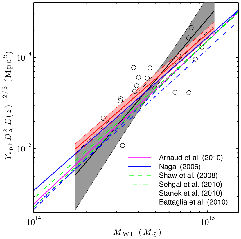
Figure 2.— Data and scaling relations at $\Delta=500$ compared to scaling relations measured from X-ray data and numerical simulations of galaxy clusters. The scaling relation fits, plotted as in Figure 1, are truncated at the boundaries of the mass range of the cluster sample including 1$\sigma$ uncertainty. Data points from this work are shown as open circles without error bars. Five simulated scaling relations between $Y_{\mathrm{sph}}$ and true $M_{\mbox{\scriptsize 500}}$ are shown, as well as the scaling relation predicted by Arnaud et al. (2010) from X-ray observations and numerical simulations. The Nagai (2006) scaling relation was derived from simulated clusters with mass greater than $10^{14}$ M_⊙, while the Sehgal et al. (2010) relation was determined from simulated $M_{\mbox{\scriptsize 500}}$$>2\times 10^{14}$ M_⊙clusters.

5.2. Observed Scatter and Morphological Segregation

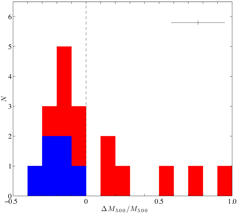
Figure 3.— Distribution of fractional deviation in mass at $\Delta=500$ of the 18 clusters in our sample from the best-fit self-similar scaling relation fit shown as the solid red line in the right panel of Fig. 1. Disturbed clusters (blue; defined in §3.3) lie exclusively on the low-mass side of the mean relation; undisturbed clusters (red) lie on both sides of the mean relation, with a tail to large positive deviations. A typical error bar for the fractional deviation is show in the upper right.

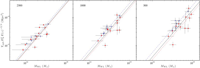
Figure 4.— The mass-$Y$ scaling relation at each overdensity, with cluster morphology indicated by the data symbols. Disturbed clusters are marked with open squares and undisturbed clusters with filled circles. The self-similar fit for the full sample is shown with a solid (black) line, and the self-similar fits to the undisturbed (red dashed) and disturbed (blue dot-dashed) subsamples are also shown.

The distribution of fractional deviations in mass ($\Delta M_{\Delta}/M_{\Delta}$) of clusters from the mean $M_{\Delta}-\mbox{$Y_{\mathrm{sph}}$}$ relations is asymmetric, particularly at $\Delta=500$ (Figure 3), where it peaks to the low-mass side of the relations (negative deviations) and has an extended tail to the high-mass side (positive deviations). Interestingly, the clusters classified as “disturbed” on the basis of the centroid shift measurements discussed in §3.3 all have $\Delta\mbox{$M_{\mbox{\scriptsize 500}}$}/\mbox{$M_{\mbox{\scriptsize 500}}$}<0$, and the tail of the distribution at $\Delta\mbox{$M_{\mbox{\scriptsize 500}}$}/\mbox{$M_{\mbox{\scriptsize 500}}$}>0.3$ comprises solely undisturbed clusters (compare the blue and red in Figure 3). This suggests that the large intrinsic scatter in our mass-$Y_{\mathrm{sph}}$ relations may be related to cluster morphology.

We detect a significant difference in the normalization of the self-similar mass-$Y_{\mathrm{sph}}$ relations between disturbed and undisturbed clusters at all three overdensity radii. At fixed $Y_{\mathrm{sph}}$, the mass of undisturbed clusters exceeds that of disturbed clusters by $13\pm 6\%$, $28\pm 5\%$, and $41\pm 6\%$ at $\Delta=2500$, 1000, and 500, respectively (Table 4.3; Figure 4). The probability of observing such an offset randomly is low even in scattered data like these; drawing random samples (with replacement) of 6 and 12 clusters from our data and repeating our fits, we find that only $1\%$ of random sub-samples are more significantly offset than the real data at $r_{\mbox{\scriptsize 500}}$.

If confirmed as a real physical effect, the morphological segregation of clusters in the mass-$Y_{\mathrm{sph}}$ plane would have major implications for SZ surveys, which expect to produce nearly mass-limited cluster samples minimally biased with respect to dynamical state. However, morphological segregation has not been seen in mass-$Y_{\mathrm{sph}}$ relations predicted from numerical simulations. Indeed, it has generally been found that the SZ signal is a robust mass proxy (merging and non-merging clusters are co-located in the mass-$Y_{\mathrm{sph}}$ plane) even during periods of mass accretion (e.g., Motl et al., 2005; Poole et al., 2007).

Simulations of merging clusters do find that cluster mergers produce transitory boosts in the SZ signal, although when integrated over the entire cluster these boosts are small and short-lived (Poole et al., 2007; Wik et al., 2008). For example, Poole et al. showed that for most merger mass ratios and relative velocities, the observed $Y$ is usually below the final “post-merger” value during the merger. This is a natural consequence of the finite time required to heat the ICM to the higher equilibrated temperature of the post-merger halo. The observational signature of this effect is that at fixed post-merger halo mass, merging (disturbed) clusters should have $Y$ suppressed relative to non-merging (undisturbed) clusters. These theoretical predictions are in the opposite sense to the morphological segregation detected in our observed mass-$Y_{\mathrm{sph}}$ relations.

5.3. Correlation of Mass and $Y$ Measurements

The ideal scaling relation measurement compares two observables that have been derived independently. X-ray scaling relations have typically been constructed from HSE-based masses derived from the same X-ray data that appear in the observable axis. HSE-based scaling relations therefore inevitably suffer varying degrees of correlation that depend on the details of the measurement methods and the observable against which mass is plotted (e.g., Mantz et al., 2010a). This correlation acts to suppress the scatter inferred for HSE-based scaling relations.

The $M_{\mathrm{WL}}$ and $Y_{\mathrm{sph}}$ measurements presented in §3 are also not completely independent, as the outer integration boundaries for the SZ profile are set by the lensing-derived overdensity radii. This introduces a correlation between observables. The mass error ($\delta M\equiv M_{WL}-M_{true}$) for an individual cluster corresponds to an error in the overdensity radius ($\delta r$),

$$\delta M=4\pi r^{2}\rho(r)\delta r~{},$$ (7)

and this error is transferred to the calculation of $Y_{\mathrm{sph}}$. Equation 7 can be converted to an equation involving fractional errors in $M$ and $r$ by dividing by $M(r)=4\pi r^{3}\bar{\rho}$/3,

$$\delta(log(M))=3\frac{\rho(r)}{\bar{\rho}}\delta(log(r))~{}.$$ (8)

The perturbation in the calculated $Y_{\mathrm{sph}}$ introduced by $\delta r$ follows the same form as equation 8, with the pressure substituted for $\rho$ and $Y_{\mathrm{sph}}$ for $M$.

From the equations for the logarithmic radial slopes of $M$ and $Y_{\mathrm{sph}}$ we can infer the response of these two quantities to the errors in $r_{\Delta}$. The direction of motion in the $M_{\mathrm{WL}}$$-$$Y_{\mathrm{sph}}$ plane for an error $\delta r$, expressed as the slope $\delta log(M)/\delta log(Y)$, is just the ratio of the logarithmic slopes in density ($\delta log(M)/\delta log(r)$) and pressure at the radius of interest. This ratio varies from cluster to cluster and across overdensities, in the present sample, it is (on average) 2.3 at $r_{\mbox{\scriptsize 2500}}$, but 1.7 at $r_{\mbox{\scriptsize 500}}$. The latter is very close to the slope of the self-similar scaling relation, $1/B=5/3$. On average then, the scatter between $M_{WL}$ and $M_{true}$ leads to errors in the derived $Y_{\mathrm{sph}}$ that move the clusters along the scaling relation at $r_{\mbox{\scriptsize 500}}$.

It was noted in §4.3 that the scatter between the mass derived from the WL shear profile fitting technique and the true cluster mass is expected to be $\sim$20% (Becker & Kravtsov, 2011), which matches the values in Table 4.3. That the observed and predicted scatter agree so well may be coincidence; simulations suggest that the astrophysics of the ICM can contribute another 10-15% scatter between $Y$ and true mass, and systematic effects like those discussed in subsequent sections can be expected to further increase the observed scatter. The above analysis suggests that $\sigma_{M|Y}$ could be larger if the $Y_{\mathrm{sph}}$ and $M_{\mathrm{WL}}$ measurements were decoupled. The clusters in this sample all have Chandra data, which provides us with an independent measurement of $r_{\mbox{\scriptsize 500}}$ for the calculation of $Y_{\mathrm{sph}}$. Using the X-ray values of $r_{\mbox{\scriptsize 500}}$ from Sanderson et al. (2009) as integration radii for both the NFW-halo fits to the weak lensing data and the SZ profiles, we again find the 20% scatter in the scaling relation. When these radii are used for the SZ data alone, the scatter increases to 26%. The coupling between observables through the integration radius therefore does appear to lessen the observed scatter, and the scatter of fully independent measurements may be more representative of the true intrinsic scatter.

5.4. Choice of Pressure Profile

Reliable measurements of $Y_{\mathrm{sph}}$ depend on the appropriate choice of pressure profile shape in the ICM models. Systematic errors in the choice of pressure profile may propagate to systematic errors in $Y_{\mathrm{sph}}$ measurements, and thus contribute to the observed scatter and segregation. Our $Y_{\mathrm{sph}}$ measurements employ the Arnaud et al. (2010) average pressure profile. However, these authors noted that CC clusters have more concentrated pressure profiles than disturbed clusters.

As a test of the importance of the profile choice on our SZ measurements, we recalculate our $Y_{\mathrm{sph}}$ values using the morphology-specific pressure profiles presented in Arnaud et al. (2010). For clusters we classify as “disturbed” and “undisturbed” we use the Arnaud et al. “morphologically disturbed” and “cool-core” profiles, respectively. The change in profile leads to small systematic changes, the disturbed clusters decrease in $Y_{\mathrm{sph}}$ by 1% and 3% at $r_{\mbox{\scriptsize 2500}}$ and $r_{\mbox{\scriptsize 500}}$, respectively, and undisturbed clusters increase by 1% and 5% at these radii. These changes can, at most, reduce the morphological segregation in the $\mbox{$M_{\mbox{\scriptsize 500}}$}-\mbox{$Y_{\mathrm{sph}}$}$ relation from $41\%$ to $31\%$.

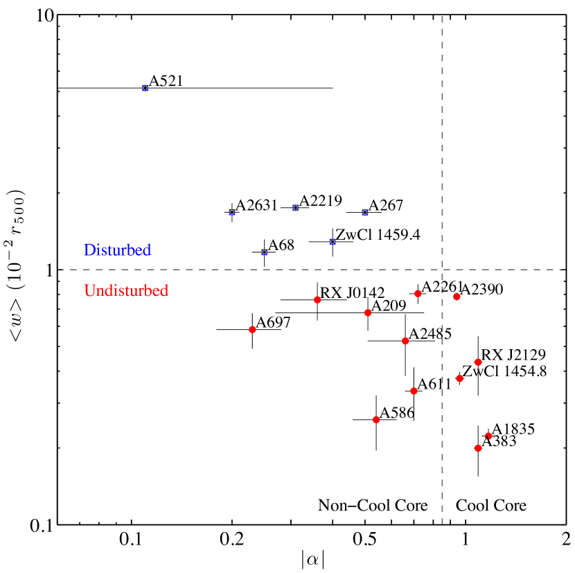
Figure 5.— X-ray centroid shift versus slope of the gas density profile at $0.04\mbox{$r_{\mbox{\scriptsize 500}}$}$ ($|\alpha|$). The density slopes are taken from Sanderson et al. (2009), where $\alpha<-0.85$ provided a reliable dividing line between cool-core and non-cool core clusters.

We expect this decrease in morphological segregation to be an upper limit on the effect of pressure profile choice on our results. Although we use the Arnaud et al. (2010) pressure profile for all of our undisturbed clusters, not all of them host a cool core (Figure 5). In the original measurement of the CC profile, Arnaud et al. excluded undisturbed clusters that lacked cool cores from their subsample, and these excluded clusters had profiles closest to the one we adopted in §3.2. We therefore conclude that although up to one fourth of the morphological segregation can be attributed to systematic errors in $Y_{\mathrm{sph}}$ due to incorrect pressure profile choice in the ICM models, the majority of the segregation remains to be explained.

5.5. Choice of Weak-lensing Mass Model

Reliable measurements of $M_{\rm WL}$ also depend on appropriate model choice. The weak-lensing masses used in this article are based on the initial Ok10 analysis of data from our Subaru observing program, in which the mass distribution of each cluster was described by a model containing a single spherical NFW halo (§3.1). We therefore explore whether this choice may contribute to the morphological segregation in the $M_{\mathrm{WL}}$$-$$Y_{\mathrm{sph}}$ plane.

Additional halos that might be justified by the data include sub-halos within each cluster, and large-scale structure projected along the same line-of-sight. We attempt the lowest order correction to our lensing analysis by adding a second dark matter halo to each mass model at the position of the most significant sub-peak in each of the density maps presented in Appendix 1 of Ok10. These 2-halo models were fitted to the 2-dimensional weak-shear field using lenstool (Jullo et al., 2007). Comparing these models to the original 1-halo models, we found that the Bayesian evidence ratio significantly favored a two-halo model for all but 3 clusters. We re-calculated $M_{\rm WL}$ at $\Delta=500$ for each cluster using the more probable of the two models, excluding the sub-halo if it is known to lie outside the cluster (e.g., RXJ 0153.2$+$0102 adjacent to A 267; see Figure 21 in Ok10), and assuming that the projected separation of the two halos is the true three-dimensional separation of the halos in all other cases. In the resulting $M_{\mbox{\scriptsize 500}}$-$Y_{\mathrm{sph}}$ scaling relation we find that neither the scatter nor segregation are reduced within the uncertainties.

The one-dimensional radial profiles used to model the cluster weak-lensing signal may also be a source of scatter. Oguri et al. (2010) fitted elliptical weak-lensing mass models to Ok10’s data, thus relaxing the assumption of azimuthal symmetry in the single NFW halo of the latter’s models. We find that the scatter and segregation in the $M_{\mathrm{WL}}$$-$$Y_{\mathrm{sph}}$ relation are all unchanged within the uncertainties if Oguri et al.’s masses are substituted for Ok10’s masses. Both of these tests suggest that the description of the projected mass distribution is not the dominant source of scatter.

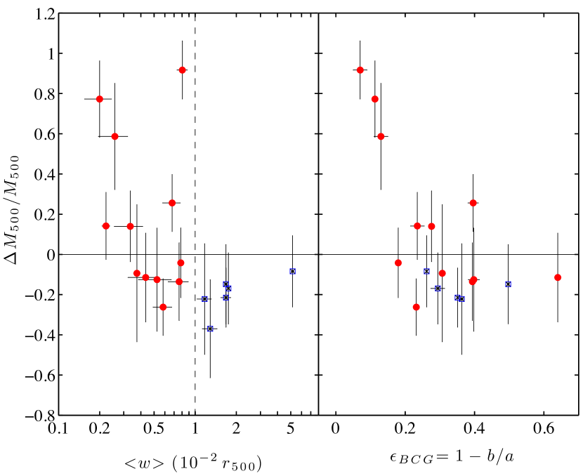
Figure 6.— Fractional deviation in mass from the SS $M_{\mbox{\scriptsize 500}}$-$Y_{\mathrm{sph}}$ relation versus centroid shift $\left<w\right>$ (left) and ellipticity of the BCG in each cluster (right). Filled circles (red) and open squares (blue) represent undisturbed and disturbed clusters, respectively. The classification is done according to the centroid shift value and the dividing line is marked by the vertical dashed line in the left panel.

The line-of-sight structure of the cluster dark matter is predicted to introduce systematic errors to lensing masses derived assuming a spherically symmetric profile (e.g., Corless & King, 2007; Meneghetti et al., 2010). An observational indicator of the line-of-sight elongation of the mass distribution would therefore be a powerful tool. First, we consider the X-ray centroid shift measurements upon which the disturbed/undisturbed classification was made in §3.3. We plot centroid shift versus fractional deviation in mass from the best-fit SS scaling relation in Figure 6, finding no reliable trend between the mass deviation and $\left<w\right>$. Though the large-$\left<w\right>$ clusters (disturbed) lie exclusively on the low-mass side of the relation, as noted in §5.2, the small-$\left<w\right>$ (undisturbed) clusters span a wide range in deviation ($\Delta\mbox{$M_{\mbox{\scriptsize 500}}$}/\mbox{$M_{\mbox{\scriptsize 500}}$}\sim 0-0.75$) at all centroid shift values. The largest deviations suggest that such clusters may be prolate spheroids viewed along an axis close to their major-axis (Corless & King, 2007), while the smallest deviations suggest that the dark matter in such clusters is relatively undisturbed and spherical. This implies that the interpretation of small centroid shifts is degenerate between a relatively undisturbed ICM and the disturbed ICM of a prolate cluster whose major axis is closely aligned with the line-of-sight. A “cleaner” indicator of the orientation of cluster dark matter halos is therefore required.

BCGs are prolate stellar systems with their major axis closely aligned with the major axis of the cluster dark matter halo and ICM (e.g., Hashimoto et al., 2008; Fasano et al., 2010). The major axis of a prolate BCG that is measured to be strongly elliptical in projection on the sky likely lies close to the plane of the sky, and thus so too does the major axis of the cluster dark matter halo. An almost circular BCG, on the other hand, indicates that the major axis is close to the line-of-sight through the cluster. BCG ellipticity measurements are available from surface photometry of Hubble Space Telescope (HST) observations of 15 of the 18 clusters in our sample (Smith et al., 2010). We analyzed two of the remaining clusters (RX J0142.0$+$2131 and A 697) in the same manner (the last cluster, ZwCl 1459.4$+$4240, has not been observed with HST). We find that the clusters with the roundest BCGs suffer the strongest positive deviations from the $M_{\mathrm{WL}}$$-$$Y_{\mathrm{sph}}$ relation, and that clusters with the most elliptical BCGs suffer negative deviations (right panel of Figure 6). Most significantly, clusters with $\epsilon_{\rm BCG}<0.15$ have exclusively large deviations ($\Delta\mbox{$M_{\mbox{\scriptsize 500}}$}/\mbox{$M_{\mbox{\scriptsize 500}}$}\mathrel{\hbox{\hbox to0.0pt{\hbox{\lower 4.0pt\hbox{$\sim$}}\hss}\hbox{$>$}}}0.5$). The mean deviation of these “round” BCGs ($\epsilon<0.15$) is $\langle\Delta\mbox{$M_{\mbox{\scriptsize 500}}$}/\mbox{$M_{\mbox{\scriptsize 500}}$}\rangle=0.76\pm 0.17$ and of “elliptical”BCGs ($\epsilon>0.15$) is $\langle\Delta\mbox{$M_{\mbox{\scriptsize 500}}$}/\mbox{$M_{\mbox{\scriptsize 500}}$}\rangle=-0.10\pm 0.17$, where the error bars are the $1\sigma$ standard deviations on the means.

The correlation between $\Delta\mbox{$M_{\mbox{\scriptsize 500}}$}/\mbox{$M_{\mbox{\scriptsize 500}}$}$ and $\epsilon_{\mathrm{BCG}}$ is strikingly similar to the trend between $M_{\mathrm{3D,WL}}/M_{\mathrm{3D,true}}$ and viewing angle in the numerically simulated clusters presented in Meneghetti et al. (2010). Indeed, visual inspection of Meneghetti et al.’s Figure 17 suggests that we are viewing clusters with “round” BCGs within $\sim 20-30^{\circ}$ of the major axis of the cluster inertia ellipsoid, and with “elliptical” BCGs at larger viewing angles. An observed BCG ellipticity of $\epsilon_{\mathrm{BCG}}=0.15$ (corresponding to an observed axis ratio of $q=b/a=0.85$) can be converted to a viewing angle with respect to the major axis by assuming an intrinsic BCG axis ratio ($\beta$). We adopt $\beta=0.67$, following the measurements of Fasano et al. (2010). The viewing angle is then estimated to be:

$$\psi=\arccos\left(\!\sqrt{\frac{1-(\beta/q)^{2}}{1-\beta^{2}}}\,\,\right)\simeq 34^{\circ}$$ (9)

which is consistent with the visual comparison of our Figure 6 and Figure 17 of Meneghetti et al. (2010).

Additional anecdotal support for this picture comes from detailed measurements of the three dimensional structure of Abell 383, which is the cluster with the second largest value of $\Delta\mbox{$M_{\mbox{\scriptsize 500}}$}/\mbox{$M_{\mbox{\scriptsize 500}}$}$ in our sample and the outlier with the greatest effect on our scaling relation fits (the lowest-$Y_{\mathrm{sph}}$ cluster in Figure 1). Newman et al. (2011) combined strong and weak lensing data, stellar kinematics in the BCG, and X-ray data to infer the three-dimensional shape of the cluster dark matter halo. They found that the cluster is very elongated along the line of sight, with an axis ratio of 2:1 between the line of sight and plane of sky. This agrees well with our inference that halo orientation is significantly affecting our weak lensing masses.

5.6. Implications for Scaling Relation Calibration

Our data provide observational support for previous numerical studies that have highlighted projection effects as an important source of systematic uncertainties in weak-lensing cluster mass measurements. These uncertainties arise from both the underlying shape of the main cluster halo and sub-halos that reside within the cluster due to a merger and/or in the surrounding large-scale structure. Future progress on the use of weak-lensing to calibrate mass-observable scaling relations will therefore benefit from intrinsically asymmetric lens models that include halo triaxiality and/or multiple halos. Direct measurements of the ratio of the line-of-sight depth to the plane-of-sky size of the cluster through joint X-ray and SZ measurements of the ICM may aid in constructing a more three-dimensional halo model. These efforts should lead to a reduction in the scatter and segregation in the $M_{\rm WL}-\mbox{$Y_{\mathrm{sph}}$}$ relation.

While the mass scatter observed here is plausibly consistent with that predicted by lensing simulations, correlated scatter between mass and $Y_{\mathrm{sph}}$ due to halo orientation and nearby structure will affect the scatter measured in scaling analyses like ours. Both the SZ and lensing signals can be expected to suffer projection effects operating in the same direction, which will reduce the scatter observed between $Y_{\mathrm{sph}}$ and $M_{\mathrm{WL}}$ from that predicted for $M_{\rm WL}-M_{\rm true}$ in lensing simulations. The SZ projection effects differ from the lensing projection in important ways, which prevents perfect cancellation of the scatter. First, the ICM (in equilibrium) will follow isopotential contours rather than isodensity contours (Buote & Canizares, 1992), which makes it much rounder than the dark matter. Lee & Suto (2003) show that the expected ICM eccentricity is typically 0.6 times that of the dark matter, corresponding to an ICM axis ratio of 1.2:1 for a matter axis ratio of 2:1. Lau et al. (2011) show that for simulated clusters the ICM is typically more spherical than either the dark matter or the potential at $r_{\mbox{\scriptsize 500}}$. Second, the SZ signal also depends on the ICM temperature, so that nearby but as-of-yet unassimilated halos will have a lower SZ signal per unit mass than the same material once it has passed through the virial shock of the main halo. For this reason, projection of adjacent halos is a weaker effect for the SZ signal. Determinations of the scatter between $Y_{\mathrm{sph}}$ and mass, as well as attempts at normalizing the $Y_{\mathrm{sph}}$-mass scaling relation using weak lensing, will need to constrain the covariance of the two observables (e.g., Allen et al., 2011).

6. Conclusions

Surveys of galaxy clusters using the SZ effect require a well-calibrated mass-observable scaling relation in order to constrain cosmological parameters. In this paper we report the first comparison of the SZ observable $Y_{\mathrm{sph}}$ with the weak lensing-determined halo mass. We find a strong correlation, and our best-fit scaling relation is consistent with expectations from self-similarity arguments (Table 4.3). Comparing to previous scaling relations measured against hydrostatic masses, our normalization at $r_{\mbox{\scriptsize 2500}}$ is consistent with that of Bonamente et al. (2008) but at $r_{\mbox{\scriptsize 500}}$ it mildly differs from SPT results presented by Andersson et al. (2011). The scatter in our relation is larger than predicted in simulations of the SZ signal, though it is not unexpected given the difficulties inherent in deriving spherical masses from the natively two-dimensional weak lensing measurements.

We considered the morphology dependence of the $M_{\mathrm{WL}}$$-$$Y_{\mathrm{sph}}$ relation by dividing our sample into undisturbed and disturbed sub-samples based on the well-established centroid shift parameter. We found that clusters segregate in the $M_{\mathrm{WL}}$$-$$Y_{\mathrm{sph}}$ plane: the mass of undisturbed clusters exceeds that of disturbed clusters at fixed $Y_{\mathrm{sph}}$. This effect becomes more pronounced at larger radii (see Table 4.3), at $\Delta=500$ undisturbed clusters are 30 – 40% more massive than disturbed clusters. Such a segregation is not predicted by numerical simulations for comparisons of the SZ signal and true cluster mass. We discuss a wide-range of possible interpretations of the segregation, and conclude that the relative simplicity of the models fitted to the data is the most likely cause. No more than one fourth of the segregation can be attributed to morphological biases introduced by the adoption of a single (morphologically blind) pressure profile in the SZ data analysis. We infer that much of the segregation is caused by modeling intrinsically prolate cluster dark matter halos as spherical objects when determining weak lensing masses from our data. This assertion is supported by the similarity between our measurements and predictions of projection-induced scatter for weak lensing data of similar quality, and the correlation we observe between BCG ellipticity, a proxy for halo orientation, and offset from our mean scaling relation. Future uses of weak lensing as a calibration tool will therefore likely be aided by attempts to correct for halo orientation, and we will explore this in the analysis of a larger sample of objects in a future paper.

References

- Akritas & Bershady (1996) Akritas, M. G., & Bershady, M. A. 1996, ApJ, 470, 706
- Allen et al. (2001) Allen, S. W., Ettori, S., & Fabian, A. C. 2001, MNRAS, 324, 877
- Allen et al. (2011) Allen, S. W., Evrard, A. E., & Mantz, A. B. 2011, ARA&A, 49, 409
- Andersson et al. (2011) Andersson, K., et al. 2011, ApJ, 738, 48
- Arnaud et al. (2010) Arnaud, M., Pratt, G. W., Piffaretti, R., Böhringer, H., Croston, J. H., & Pointecouteau, E. 2010, A&A, 517, A92
- Bardeau et al. (2007) Bardeau, S., Soucail, G., Kneib, J.-P., Czoske, O., Ebeling, H., Hudelot, P., Smail, I., & Smith, G. P. 2007, A&A, 470, 449
- Battaglia et al. (2010) Battaglia, N., Bond, J. R., Pfrommer, C., Sievers, J. L., & Sijacki, D. 2010, ApJ, 725, 91
- Becker & Kravtsov (2011) Becker, M. R., & Kravtsov, A. V. 2011, ApJ, 740, 25
- Becker et al. (1995) Becker, R. H., White, R. L., & Helfand, D. J. 1995, ApJ, 450, 559
- Böhringer et al. (2004) Böhringer, H., et al. 2004, A&A, 425, 367
- Böhringer et al. (2010) —. 2010, A&A, 514, A32
- Bonamente et al. (2008) Bonamente, M., Joy, M., LaRoque, S. J., Carlstrom, J. E., Nagai, D., & Marrone, D. P. 2008, ApJ, 675, 106
- Bonamente et al. (2006) Bonamente, M., Joy, M. K., LaRoque, S. J., Carlstrom, J. E., Reese, E. D., & Dawson, K. S. 2006, ApJ, 647, 25
- Bryan & Norman (1998) Bryan, G. L., & Norman, M. L. 1998, ApJ, 495, 80
- Buote & Canizares (1992) Buote, D. A., & Canizares, C. R. 1992, ApJ, 400, 385
- Burns et al. (2010) Burns, J. O., Skillman, S. W., & O’Shea, B. W. 2010, ApJ, 721, 1105
- Carlstrom et al. (2002) Carlstrom, J. E., Holder, G. P., & Reese, E. D. 2002, ARA&A, 40, 643
- Cavaliere et al. (2011) Cavaliere, A., Lapi, A., & Fusco-Femiano, R. 2011, A&A, 525, A110
- Corless & King (2007) Corless, V. L., & King, L. J. 2007, MNRAS, 380, 149
- Culverhouse et al. (2010) Culverhouse, T. L., et al. 2010, ApJ, 723, L78
- da Silva et al. (2004) da Silva, A. C., Kay, S. T., Liddle, A. R., & Thomas, P. A. 2004, MNRAS, 348, 1401
- Dahle et al. (2002) Dahle, H., Kaiser, N., Irgens, R. J., Lilje, P. B., & Maddox, S. J. 2002, ApJS, 139, 313
- Ebeling et al. (2000) Ebeling, H., Edge, A. C., Allen, S. W., Crawford, C. S., Fabian, A. C., & Huchra, J. P. 2000, MNRAS, 318, 333
- Ebeling et al. (1998) Ebeling, H., Edge, A. C., Bohringer, H., Allen, S. W., Crawford, C. S., Fabian, A. C., Voges, W., & Huchra, J. P. 1998, MNRAS, 301, 881
- Fasano et al. (2010) Fasano, G., et al. 2010, MNRAS, 404, 1490
- Giovannini et al. (2009) Giovannini, G., Bonafede, A., Feretti, L., Govoni, F., Murgia, M., Ferrari, F., & Monti, G. 2009, A&A, 507, 1257
- Giovannini et al. (1987) Giovannini, G., Feretti, L., & Gregorini, L. 1987, A&AS, 69, 171
- Haarsma et al. (2010) Haarsma, D. B., et al. 2010, ApJ, 713, 1037
- Hashimoto et al. (2008) Hashimoto, Y., Henry, J. P., & Boehringer, H. 2008, MNRAS, 390, 1562
- Hicken et al. (2009) Hicken, M., Wood-Vasey, W. M., Blondin, S., Challis, P., Jha, S., Kelly, P. L., Rest, A., & Kirshner, R. P. 2009, ApJ, 700, 1097
- Hoekstra (2001) Hoekstra, H. 2001, A&A, 370, 743
- Hoekstra (2003) —. 2003, MNRAS, 339, 1155
- Hoekstra (2007) —. 2007, MNRAS, 379, 317
- Hoekstra et al. (2011) Hoekstra, H., Donahue, M., Conselice, C. J., McNamara, B. R., & Voit, G. M. 2011, ApJ, 726, 48
- Holder et al. (2007) Holder, G. P., McCarthy, I. G., & Babul, A. 2007, MNRAS, 382, 1697
- Ilbert et al. (2009) Ilbert, O., et al. 2009, ApJ, 690, 1236
- Jullo et al. (2007) Jullo, E., Kneib, J.-P., Limousin, M., Elíasdóttir, Á., Marshall, P. J., & Verdugo, T. 2007, New Journal of Physics, 9, 447
- Kaiser (1986) Kaiser, N. 1986, MNRAS, 222, 323
- Kaiser et al. (1995) Kaiser, N., Squires, G., & Broadhurst, T. 1995, ApJ, 449, 460
- Kelly (2007) Kelly, B. C. 2007, ApJ, 665, 1489
- Kessler et al. (2009) Kessler, R., et al. 2009, ApJS, 185, 32
- Komatsu et al. (2011) Komatsu, E., et al. 2011, ApJS, 192, 18
- Lau et al. (2009) Lau, E. T., Kravtsov, A. V., & Nagai, D. 2009, ApJ, 705, 1129
- Lau et al. (2011) Lau, E. T., Nagai, D., Kravtsov, A. V., & Zentner, A. R. 2011, ApJ, 734, 93
- Lee & Suto (2003) Lee, J., & Suto, Y. 2003, ApJ, 585, 151
- Mahdavi et al. (2008) Mahdavi, A., Hoekstra, H., Babul, A., & Henry, J. P. 2008, MNRAS, 384, 1567
- Mantz et al. (2010a) Mantz, A., Allen, S. W., Ebeling, H., Rapetti, D., & Drlica-Wagner, A. 2010a, MNRAS, 406, 1773
- Mantz et al. (2010b) Mantz, A., Allen, S. W., Rapetti, D., & Ebeling, H. 2010b, MNRAS, 406, 1759
- Marriage et al. (2011) Marriage, T. A., et al. 2011, ApJ, in press, arXiv:1010.1065
- Marrone et al. (2009) Marrone, D. P., et al. 2009, ApJ, 701, L114
- Maughan et al. (2008) Maughan, B. J., Jones, C., Forman, W., & Van Speybroeck, L. 2008, ApJS, 174, 117
- Mazzotta et al. (2001) Mazzotta, P., Markevitch, M., Vikhlinin, A., Forman, W. R., David, L. P., & van Speybroeck, L. 2001, ApJ, 555, 205
- Meneghetti et al. (2010) Meneghetti, M., Rasia, E., Merten, J., Bellagamba, F., Ettori, S., Mazzotta, P., Dolag, K., & Marri, S. 2010, A&A, 514, A93
- Metzler et al. (2001) Metzler, C. A., White, M., & Loken, C. 2001, ApJ, 547, 560
- Mohr et al. (1995) Mohr, J. J., Evrard, A. E., Fabricant, D. G., & Geller, M. J. 1995, ApJ, 447, 8
- Motl et al. (2005) Motl, P. M., Hallman, E. J., Burns, J. O., & Norman, M. L. 2005, ApJ, 623, L63
- Mroczkowski et al. (2009) Mroczkowski, T., et al. 2009, ApJ, 694, 1034
- Nagai (2006) Nagai, D. 2006, ApJ, 650, 538
- Nagai et al. (2007) Nagai, D., Kravtsov, A. V., & Vikhlinin, A. 2007, ApJ, 668, 1
- Navarro et al. (1996) Navarro, J. F., Frenk, C. S., & White, S. D. M. 1996, ApJ, 462, 563
- Newman et al. (2011) Newman, A. B., Treu, T., Ellis, R. S., & Sand, D. J. 2011, ApJ, 728, L39
- Oguri et al. (2010) Oguri, M., Takada, M., Okabe, N., & Smith, G. P. 2010, MNRAS, 405, 2215
- Okabe et al. (2010a) Okabe, N., Takada, M., Umetsu, K., Futamase, T., & Smith, G. P. 2010a, PASJ, 62, 811
- Okabe et al. (2010b) Okabe, N., Zhang, Y., Finoguenov, A., Takada, M., Smith, G. P., Umetsu, K., & Futamase, T. 2010b, ApJ, 721, 875
- Percival et al. (2010) Percival, W. J., et al. 2010, MNRAS, 401, 2148
- Plagge et al. (2010) Plagge, T., et al. 2010, ApJ, 716, 1118
- Planck Collaboration et al. (2011) Planck Collaboration et al. 2011, A&A, 536, A8
- Poole et al. (2007) Poole, G. B., Babul, A., McCarthy, I. G., Fardal, M. A., Bildfell, C. J., Quinn, T., & Mahdavi, A. 2007, MNRAS, 380, 437
- Pratt et al. (2009) Pratt, G. W., Croston, J. H., Arnaud, M., & Böhringer, H. 2009, A&A, 498, 361
- Rasia et al. (2006) Rasia, E., et al. 2006, MNRAS, 369, 2013
- Rudy et al. (1987) Rudy, D. J., Muhleman, D. O., Berge, G. L., Jakosky, B. M., & Christensen, P. R. 1987, Icarus, 71, 159
- Rykoff et al. (2008) Rykoff, E. S., et al. 2008, MNRAS, 387, L28
- Sanderson et al. (2009) Sanderson, A. J. R., Edge, A. C., & Smith, G. P. 2009, MNRAS, 398, 1698
- Schmidt et al. (2001) Schmidt, R. W., Allen, S. W., & Fabian, A. C. 2001, MNRAS, 327, 1057
- Sehgal et al. (2010) Sehgal, N., Bode, P., Das, S., Hernandez-Monteagudo, C., Huffenberger, K., Lin, Y., Ostriker, J. P., & Trac, H. 2010, ApJ, 709, 920
- Sehgal et al. (2011) Sehgal, N., et al. 2011, ApJ, 732, 44
- Sharp et al. (2010) Sharp, M. K., et al. 2010, ApJ, 713, 82
- Shaw et al. (2008) Shaw, L. D., Holder, G. P., & Bode, P. 2008, ApJ, 686, 206
- Smith et al. (2001) Smith, G. P., Kneib, J.-P., Ebeling, H., Czoske, O., & Smail, I. 2001, ApJ, 552, 493
- Smith et al. (2005) Smith, G. P., Kneib, J.-P., Smail, I., Mazzotta, P., Ebeling, H., & Czoske, O. 2005, MNRAS, 359, 417
- Smith et al. (2010) Smith, G. P., et al. 2010, MNRAS, 409, 169
- Stanek et al. (2010) Stanek, R., Rasia, E., Evrard, A. E., Pearce, F., & Gazzola, L. 2010, ApJ, 715, 1508
- Staniszewski et al. (2009) Staniszewski, Z., et al. 2009, ApJ, 701, 32
- Tremaine et al. (2002) Tremaine, S., et al. 2002, ApJ, 574, 740
- Umetsu & Broadhurst (2008) Umetsu, K., & Broadhurst, T. 2008, ApJ, 684, 177
- Umetsu et al. (2009) Umetsu, K., et al. 2009, ApJ, 694, 1643
- Vanderlinde et al. (2010) Vanderlinde, K., et al. 2010, ApJ, 722, 1180
- Vikhlinin et al. (2006) Vikhlinin, A., Kravtsov, A., Forman, W., Jones, C., Markevitch, M., Murray, S. S., & Van Speybroeck, L. 2006, ApJ, 640, 691
- Vikhlinin et al. (2009a) Vikhlinin, A., et al. 2009a, ApJ, 692, 1033
- Vikhlinin et al. (2009b) —. 2009b, ApJ, 692, 1060
- Weiner et al. (2006) Weiner, B. J., et al. 2006, ApJ, 653, 1049
- Wik et al. (2008) Wik, D. R., Sarazin, C. L., Ricker, P. M., & Randall, S. W. 2008, ApJ, 680, 17
- Williamson et al. (2011) Williamson, R., et al. 2011, ApJ, 738, 139
- Zhang et al. (2010) Zhang, Y., et al. 2010, ApJ, 711, 1033
- Zhang et al. (2007) Zhang, Y.-Y., Finoguenov, A., Böhringer, H., Kneib, J.-P., Smith, G. P., Czoske, O., & Soucail, G. 2007, A&A, 467, 437
- Zhang et al. (2008) Zhang, Y.-Y., Finoguenov, A., Böhringer, H., Kneib, J.-P., Smith, G. P., Kneissl, R., Okabe, N., & Dahle, H. 2008, A&A, 482, 451