Dynamical tunneling and control

Abstract

Contribution to the edited volume Dynamical Tunneling: Theory and Experiment, Editors Srihari Keshavamurthy and Peter Schlagheck, CRC Press , Taylor & Francis, Boca Raton, 2011.

I Introduction

Tunneling is a supreme quantum effect. Every introductory textintroqmbook on quantum mechanics gives the paradigm example of a particle tunneling through a one-dimensional potential barrier despite having a total energy less than the barrier height. Indeed, the reader typically works through a number of excercises, all involving one-dimensional potential barriers of one form or another modelling several key physical phenomena ranging from atom transfer reactions to the decay of alpha particlesmerz02 . However, one seldom encounters coupled multidimenisonal tunneling in such texts since an analytical solution of the Schrödinger equation in such cases is not possible. Interestingly, the richness and complexity of the tunneling phenomenon manifest themselves in full glory in the case of multidimensional systemsmultidtun . Thus, for instance, the usual one-dimensional expectation of increasing tunneling splittings as one approaches the barrier top from below is not necessarily true as soon as one couples another bound degree of freedom to the tunneling coordinate. In the context of molecular reaction dynamics, multidimensional tunneling can result in strong mode-specificity and fluctuations in the reaction ratesmillerpaps . In fact, a proper description of tunneling of electrons and hydrogen atoms is absolutely essentiallargemoltun ; bo2000 even in molecular systems as large as enzymes and proteins. Although one usually assumes tunneling effects to be significant in molecules involving light atom transfers it is worth pointing out that neglecting the tunneling of even a heavy atom like carbon is the difference between a reaction occuring or not occuring. In particular, one can underestimate rates by nearly hundred orders of magnitudecatomtun . Interestingly, and perhaps paradoxically, several penetrating insights into the nature and mechanism of multidimensional barrier tunneling have been obtained from a phase space perspectivecreagh ; shudo . The contributions by Creagh, Shudo and Ikeda, and Takahashi in the present volume provide a detailed account of the latest advances in the phase space based understanding of multidimensional barrier tunneling.

What happens if there are no coordinate space barriers? In other words, in situations wherein there are no static energetic barriers separating “reactants” from the “products” does one still have to be concerned about quantum tunneling? One such model potential is shown in Fig. 1 which will be discussed in the next section. Here we have the notion of reactants and products in a very general sense. So, for instance, in the context of a conformational reaction they might correspond to the several near-degenerate conformations of a specific molecule. Naively one might expect that tunneling has no consequences in such cases. However, studies over last several decadeslc79 ; dh81 ; hp84 ; Ozo84 ; srh82c ; sp87 ; gh87 ; lb90 ; btu93 ; tu94 ; df95 have revealed that things are not so straightforward. Despite the lack of static barriers, the dynamics of the system can generate barriers and quantum tunneling can occur through such dynamical barriersdtunbook1 . This, of course, immediately implies that dynamical tunneling is a very rich and subtle phenomenon since the nature and number of barriers can vary appreciably with changes in the nature of the dynamics over the timescales of interest. This would also seem to imply that deciphering the mechanism of dynamical tunneling is a hopeless task as opposed to the static potential barrier case wherein elegant approximations to the tunneling rate and splittings can be written down. However, recent studies have clearly established that even in the case of dynamical tunneling it is possible to obtain very accurate approximations to the splittings and rate. In particular, it is now clear that unambiguous identification of the local dynamical barriers is possible only by a detailed study of the structure of the underlying classical phase space. The general picture that has emerged is that dynamical tunneling connects two or more classically disconnected regions in the phase space. More importantly, and perhaps ironically, the dynamical tunneling splittings and rates are extremely sensitive to the various phase space structures like nonlinear resonancesbsu01 ; bsu02 ; seu05 ; es05 ; bfgr98 ; ablr01 ; rbiwg94 ; sfgr06 , chaosgh87 ; lb90 ; btu93 ; tu94 ; Ort96 ; ammk95 and partial barriersgrr86 ; pre00-mh-chap3 . It is crucial to note that although purely quantum approaches can be formulated for obtaining the tunneling splittings, any mechanistic understanding requires a detailed understanding of the phase space topology. In this sense, the phenomenon of dynamical tunneling gets intimately linked to issues related to phase space transport. Thus, one now has the concept of resonance-assisted tunneling (RAT) and chaos-assisted tunneling (CAT) and realistic systems typically involve both the mechanisms.

Since the appearance of the first bookdtunbook1 on the topic of interest more than a decade ago, there have been several beautiful experimental studiesns97 ; hadghhrr05 ; hetal01 ; sor01 ; bafmli03 ; shfhsn10 that have revealed various aspects of the phenomenon of dynamical tunneling. The most recent one by Chaudhury et al. realizescsagj09 the paradigmatic kicked top model using cold ¹³³Cs atoms and clearly demonstrate the dynamical tunneling occuring in the underlying phase space. Interestingly, good correspondence between the quantum dynamics and classical phase space structures is found despite the system being in a deep quantum regime. As another example, I mention the experimental observationftcfswmb07 by Fölling et al. of second order co-tunneling of interacting ultracold rubidium atoms in a double well trap. The similarities between this system and the studies on dynamical tunneling using molecular effective Hamiltonians is striking. In particular, the description of the cold atom study in terms of superexchange (qualitative and quantitative) is reminiscent of the early work by Stuchebrukhov and Marcussmdyntun93 on understanding the role of dynamical tunneling in the phenomenon of intramolecular energy flow. Further details on the experimental realizations can be found in this volume in the articles by Steck and Raizen, and Hensinger. An earlier reviewKes07 provides extensive references to the experimental manifestations of dynamical tunneling in molecular systems in terms of spectroscopic signatures. Undoubtedly, in the coming years, one can expect several other experimental studies which will lead to a deeper understanding of dynamical tunneling and raise many intriguing issues related to the subject of classical-quantum correspondence.

As remarked earlier, it seems ironic that a pure quantum effect like tunneling should bear the marks of the underlying classical phase space structures. However, it is useful to to recall the statement by Heller that tunneling is only meaningful with classical dynamics as the baseline. Thus, insights into the nature of the classical dynamics translates into a deeper mechanistic insight into the corresponding quantum dynamics. Indeed, one way of thinking about classical-quantum correspondence is that classical mechanics is providing us with the best possible “basis” to describe the quantum evolution. The wide range of contributions in this volume are a testimony to the richness of the phenomenon of dynamical tunneling and the utility of such a classical-quantum correspondence perspective. In this article I focus on the specific field of quantum control and show as to how dynamical tunneling can lead to useful insights into the control mechanismnote0 ; asthesis . The hope is that more such studies will eventually result in control strategies which are firmly rooted in the intutive classical world, yet accounting for the classically forbidden pathways and mechanisms in a consistent fashion. This is a tall order, and some may even argue as an unnecessary effort in these days of fast computers and smart and efficient algorithms to solve fairly high dimensional quantum dynamics. However, in this context, it is useful to remember the following which was written by Born, Heisenberg, and Jordan nearly eighty years agobhj

“The starting point of our theoretical approach was the conviction that the difficulties that have been encountered at every step in quantum theory in the last few years could be surmounted only by establishing a mathematical system for the mechanics of atomic and electronic motions, which would have a unity and simplicity comparable with the system of classical mechanics…further developement of the theory, an important task will lie in the closer investigation of the nature of this correspondence and in the description of the manner in which symbolic quantum geometry goes over into visualizable classical geometry.”

The above remark was made in an era when computers were nonexistent. Nevertheless, it is remarkably prescient since even in the present era one realizes the sheer difficulty in implementing an all-quantum dynamical study on even relatively small moleculeslt10 . In any case, it is not entirely unreasonable to argue that large scale quantum dynamical studies will still require some form of an implicit classical-quantum correspondence approach to grasp the underlying mechanistic details. With the above remark in mind I start things off by revisiting the original paperdh81 by Davis and Heller since, in my opinion, it is ideal from the pedagogical point of view.

II Davis-Heller system revisited

Three decades ago, Davis and Heller in their pioneering studydh81 gave a clear example of dynamical tunneling. A short recount of this work including the famous plots of the classical trajectories and the associated quantum eigenstates can be found in Heller’s article in this volume. However, I revisit this model here in order to bring forth a couple of important points that seem to have been overlooked in subsequent works. First, the existence of another class of eigenstate pairs, called as circulating statesdh81 , which can exert considerable influence on the usual tunneling doublets at higher energies. Second, a remark in the original paperdh81 which can be considered as a harbinger for chaos-assisted tunneling. As shown below, there are features in the original model that are worth studying in some detail even after three decades since the original paper was published.

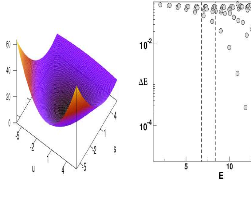
Figure 1: The left plot shows the two-dimensional potential used by Davis and Heller to illustrate the phenomenon of dynamical tunneling. Note that there are no barriers in the coordinate space. On the right the magnitude of the splitting between adjacent eigenstates are shown as a function of the eigenenergies. The first and second dotted vertical lines indicate the energies around which the symmetric (s) and unsymmetric (u) stretch modes become unstable. Sequences of doublets with very small splittings can be seen around the onset of the instabilities. On the other hand, the regularity of the sequences vanishes at higher energies.

The Hamiltonian of choice is the two degrees of freedom (2DoF, in what follows the acronymn DoF stands for degrees of freedom) Barbanis-like modeldh81

$$H(s,u,p_{s},p_{u})=\frac{1}{2}\left(p_{s}^{2}+p_{u}^{2}\right)+\frac{1}{2}\left(\omega_{s}^{2}s^{2}+\omega_{u}^{2}u^{2}\right)+\lambda su^{2}$$ (1)

with the labels ‘s’ and ‘u’ denoting the symmetric and unsymmetric stretch modes respectively. The above Hamiltonian has also been studiedhsd80 in great detail to uncover the correspondence between classical stability of the motion and quantum spectral features, wavefunctions, and energy transfer. The potential is symmetric with respect to $u\leftrightarrow-u$ as shown in Fig. 1 but there is no potential barrier. Davis and Heller used the parameter values $\omega_{s}=1.0,\omega_{u}=1.1$, and $\lambda=-0.11$ for which the dissociation energy $E_{\rm dis}\equiv\omega_{s}^{2}\omega_{u}^{4}/8\lambda^{2}=15.125$. Note that the masses are taken to be unity and one is working in units such that $\hbar=1$. The key observation by Davis and Heller was that despite the lack of any potential barriers several bound eigenstates came in symmetric-antisymmetric pairs $|\psi_{1}\rangle$ and $|\psi_{2}\rangle$ with energy splittings much smaller than the fundamental frequencies i.e., $\Delta E\equiv|E_{1}-E_{2}|\ll O(1)$. In Fig. 1 the various splittings between adjacent eigenstates are shown and it is clear that several “tunneling” pairs appear above a certain threshold energy.

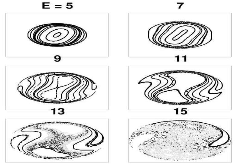
Figure 2: Evolution of the classical phase space with increasing energy shown as $(u,p_{u})$ Poincaré surface of sections. Note that large scale chaos appears for $E\geq 11$. The formation of a separatrix and two classically disjoint regular regions can be seen at $E=9$ due to the symmetric mode periodic orbit becoming unstable. The regular regions almost vanish near the dissociation energy. In the bottom row some of the chaotic orbits have been suppressed, for clarity of the figure, by showing them in gray.

How can one understand the onset of such near degeneracies in the system? The crucial insight that Davis and Heller provided was that the appearance of such doublets is correlated with the large scale changes in the classical phase space. The nature of the phase space with increasing total energy is shown in Fig. 2 using the $(u,p_{u})$ Poincaré surface of section. Such a surface of section, following standard methods, is constructed by recording the points, with momentum $p_{s}>0$, of the intersection of a trajectory with the the $s=0$ plane in the phase space. Such a procedure for several trajectories with specific total energy generates a typical surface of section as shown in Fig. 2 and clearly indicates the global nature of the phase space. It is clear from the figure that the phase space for $E<11$ is mostly regular while higher energy phase spaces exhibit mixed regular-chaotic dynamics. One of the most prominent change happens when the symmetric stretch periodic orbit $(u=0,p_{u}=0)$ becomes unstable around $E\approx 6.8$. In Fig. 2 the consequence of such a bifurcation can be clearly seen for $E=9$ as the formation of two classically disjoint regular regions. In fact, the two regular regions signal a $1$:$1$ resonance between the stretching modes. The crucial point to observe here is that classical trajectories initiated in one of the regular regions cannot evolve into the other regular region. With increasing energy the classically disjoint regular regions move further apart and almost vanish near the dissociation energy. The result presented in Fig. 1 in fact closely mirrors the topological changes, shown in Fig. 2, in the phase space. Thus, in Fig. 1 a sequence of eigenstates with very small splittings begins right around the energy at which the symmetric periodic orbit becomes unstable. The unsymmetric stretch, however, becomes unstable at a higher energy $E\approx 8.3$ and one can observe in Fig. 1 another sequence that seemingly begins near this point. Note that at higher energies it is not easy to identify any more sequences, but small splittings are still observed. The important thing to note here is that not only do the splittings but the individual eigenstates also correlate with the changes in the phase space.

In Fig. 3 we show a set of four eigenstates to illustrate an important point - as soon as the $1$:$1$ resonance manifests itself in the phase space, the tunneling doublets start to form and an integrable normal form approximation is insufficient to account for the splittings. Note that the phase space is mostly regular at the energies of interest. A much more detailed analysis can be found in the paper by Farrelly and Uzerfu86 . We begin by notingnote1 that the pair of eigenstates (counting from the zero-point) $35$ and $36$ are split by about $\Delta E\approx 6.41\times 10^{-2}$ whereas the pair $37$ and $38$ are separated by about $2.09\times 10^{-2}$. In both cases the splitting is smaller than the fundamental frequencies, which are of order unity. Note that the latter pair of states appears to be a part of the sequence in Fig. 1 that starts right after the bifurcation of the symmetric stretch periodic orbit. Since the original mode frequencies are nonresonant, one can obtain a normal form approximationfu86 to the original Hamiltonian and see if the obtained splittings can be explained satisfactorily. In other words, the observed $\Delta E$ are coming from the perturbation that couples both the modes and in such a case there is no reason for classifying them as tunneling doublets. However, from the coordinate space representations of the states shown in Fig. 3 one observes that there is an important difference between the two pairs of states. The pair $(35,36)$ seems to have a perturbed nodal structure and hence one can approximately assign the states using the zeroth-order quantum numbers $(n_{s},n_{u})$. Inspecting the figure leads to the assignment $(1,6)$ and $(0,7)$ for states $35$ and $36$ respectively. If the above arguments are correct then the splitting $\Delta E_{35,36}$ should be obtainable from the normal form Hamiltonian. Since the theory of normal forms is explained in detail in several textbookslichtlieb , I will provide a brief derivation below. Begin by using the unperturbed harmonic action-angle variables $({\bf I},{\bf\phi})$ defined via the canonical transformation (similar set for $s$ mode):

$$u = \left(\frac{2I_{u}}{\omega_{u}}\right)^{1/2}\sin\phi_{u},$$ (2)

$$p_{u} = \left(2\omega_{u}I_{u}\right)^{1/2}\cos\phi_{u},$$ (3)

to express the original Hamiltonian as

$$H({\bf I},{\bm{\phi}}) = \omega_{s}I_{s}+\omega_{u}I_{u}+\widetilde{\lambda}I_{s}^{1/2}I_{u}\left\{\sin\phi_{s}-\frac{1}{2}\sin(\phi_{s}+2\phi_{u})-\frac{1}{2}\sin(\phi_{s}-2\phi_{u})\right\}$$ (4)

$$\equiv H_{0}({\bf I})+\widetilde{\lambda}H_{1}({\bf I},{\bm{\phi}}),$$

where $\widetilde{\lambda}\equiv\lambda\sqrt{2}/(\omega_{u}\sqrt{\omega_{s}})$. Since $H_{1}$ is purely oscillatory the angle average

$$\bar{H}_{1}\equiv\frac{1}{(2\pi)^{2}}\int d{\bm{\phi}}H_{1}({\bf I},{\bm{\phi}})=0$$ (5)

and thus to $O(\widetilde{\lambda})$ the normal form Hamiltonian can be identified with the zeroth-order $H_{0}({\bf I})$ above. The first nontrivial correction arises at $O(\widetilde{\lambda}^{2})$ and can be obtained using the $O(\widetilde{\lambda})$ generating function

$$W_{1}({\bf I},{\bf\phi})=\sum_{{\bf k}\neq{\bf 0}}\frac{i}{{\bf k}\cdot{\bf\omega}}H_{1,{\bf k}}({\bf I})e^{i{\bf k}\cdot{\bf\phi}}$$ (6)

where $H_{1,{\bf k}}({\bf I})$ are the coefficients in the Fourier expansion of the oscillatory part of $H_{1}({\bf I},{\bm{\phi}})$. One now obtains the $O(\widetilde{\lambda}^{2})$ correction to the Hamiltonian as

$$K_{2}=\frac{1}{2}\overline{\{W_{1},H_{1}\}}$$ (7)

with the bar denoting angle averaging of the Poisson bracket involving $W_{1}$ and $H_{1}$. Performing the calculations the normal form at $O(\widetilde{\lambda}^{2})$ is obtained as

$$H_{N}^{(2)}=\omega_{s}I_{s}+\omega_{u}I_{u}+\widetilde{\lambda}^{2}K_{2}$$ (8)

with

$$K_{2}=\frac{1}{\omega_{s}\omega_{u}^{2}}\left[\left(\frac{2\omega_{u}}{\omega_{s}^{2}-4\omega_{u}^{2}}\right)I_{s}I_{u}-\left(\frac{3\omega_{s}^{2}-8\omega_{u}^{2}}{4\omega_{s}(\omega_{s}^{2}-4\omega_{u}^{2})}\right)I_{u}^{2}\right]$$ (9)

The primitive Bohr-Sommerfeld quantization $I_{j}\rightarrow(n_{j}+1/2)\hbar$ yields the quantum eigenvalues perturbatively to $O(\widetilde{\lambda}^{2})$. The procedure can be repeated to obtain the normal form Hamiltonian at higher orders. For instance, Farrelly and Uzer havefu86 computed the normal form out to $O(\widetilde{\lambda}^{12})$ and used Padé resummation techniques to improve in cases when the zeroth-order frequencies are near-resonant. For our qualitative discussions, the $O(\widetilde{\lambda}^{2})$ normal form is sufficient.

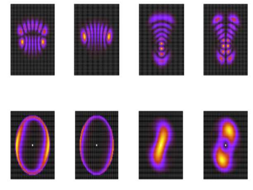
Figure 3: Four eigenstates close to an energy where the $1$:$1$ resonance is just starting to appear. The upper panel shows the $(u,s)$ coordinate space representations and the lower panels show the corresponding Husimi distributions in the $(u,p_{u})$ surface of section of the phase space. The first two states ($E\approx 8.4$) can be assigned approximate zeroth-order quantum numbers $(n_{s},n_{u})$ whereas the last two states ($E\approx 9.0$) show perturbed nodal features. Clear difference in the phase space nature of the eigenstates can be seen. See text for details.

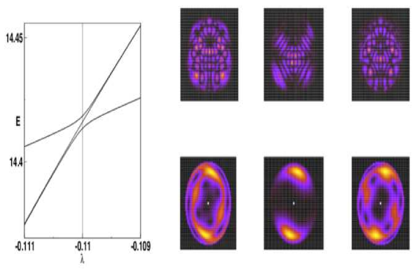
Figure 4: An avoided crossing in the high energy region ($E\approx 14.4$) of the Davis-Heller system involving three states. As in the previous figure, the $(u,s)$ and phase space Husimi representations are also shown. The first and the last states appear to be strongly mixed states. The middle state seems relatively cleaner. Does chaos play a role in this case? Detailed discussions in the text.

Notice that the normal form Hamiltonian above is integrable since it is ignorable in the angle variables. Indeed, using the normal form and the approximate assignments of the eigenstates shown in Fig. 3 one finds $\Delta E_{35,36}\approx 7.4\times 10^{-2}$ which is in fair agreement with the actual numerical value. Thus, a large part of the splitting $\Delta E_{35,36}$ can be explained classically. On the other hand, although the states $37$ and $38$ seem to have an identifiable nodal structure (cf. Fig. 3), it is clear that they are significantly perturbed. Nevertheless, persisting with an approach based on counting the nodes, states $37$ and $38$ can be assigned as $(8,0)$ and $(7,1)$ respectively. Using the normal form one estimates $\Delta E_{37,38}\approx 5.12\times 10^{-2}$ and this is about a factor of two larger than the numerically computed value. Thus, the splitting in this case is not accounted for solely by classical considerations. One might argue that a higher order normal form might lead to better agreement, but the phase space Husimi distributions of the eigenstates shown in Fig. 3 suggests otherwise. The Husimi disributions, when compared to the classical phase spaces shown in Fig. 2, clearly show that the pair $(37,38)$ are localized in the newly created $1$:$1$ resonance zone. Hence, this pair of states is directly influenced by the nonlinear resonance and the splitting between them cannot be accurately described by the normal form Hamiltonian. Indeed, as discussed by Farrelly and Uzerfu86 , in this instance one needs to consider a resonant Hamiltonian which explicitly takes the $1$:$1$ resonance into account. This provides a clear link between dynamical tunneling, appearance of closely spaced doublets and creation of new, in this case a nonlinear resonance, phase space structures. The choice of states in Fig. 3 is different from what is usually shown as the standard example for dynamical tunneling pairs. However, in the discussion above the states were chosen intentionally with the purpose of illustrating the onset of near-degeneracy due to the formation of a nonlinear resonance. In a typical situation involving near-integrable phase spaces there are several such resonances ranging from low orders to fairly high orders. The importance of a specific resonance depends sensitively on the effective value of the Planck’s constantSchl06 ; lbks10 . Indeed, detailed studiesmes06 ; Kes03 ; Kes05 have shown that excellent agreement with numerically computed splittings can be obtained if proper care is taken to include the various resonances. Clear and striking examples in this context can be found in the contributions by Schlagheck et al. and Bäcker et al. in this volume.

To finish the discussion of the Davis-Heller system I show an example which involves states forming tunneling pairs that are fairly complicated both in terms of their coordinate space representations as well as their phase space Husimi distributions. The example involves three states $102$, $103$, and $104$ around $E\approx 14.4$, which is rather close to the dissociation energy. In the original workdh81 Davis and Heller noted that the splittings seem to increase by an order of magnitude in this high energy region. Notably, they commented that “perhaps the degree of irregularity between the regular regions plays some part”. In Fig. 4 the variation of energy levels with the coupling parameter $\lambda$ is shown. One can immediately see that the three states are right at the center of an avoided crossing. The coordinate space representations of the states shows extensive mixing for states $102$ and $104$ while the state $103$ seems to be cleaner. The Husimi distributions for the respective states conveys the same message. Comparing to the phase space sections shown in Fig. 2 it is clear that the Husimis for state $102$ and $104$ seem to be ignoring the classical regular-chaotic divison - a clear indication of the quantum nature of the mixing. Although it is not possible to strictly assign these states as chaotic, a closer inspection does show substantial Husimi contribution in the border between the regular and chaotic regions. Interestingly, the pairwise splitting between the states is nearly the same but localized linear combinations of any two states exhibits two-level dynamics. Thus, the situation here is not of the genericbtu93 chaos-assisted tunneling one wherein one of the states is chaotic and interacts with the other two regular states. Nevertheless, linear combinations of the three states reveal (not shown here) that they are mixed with each other. A look at the coordinate and phase space representations of states $102$ and $104$ in Fig. 4 reveals that a different kind of state is causing the three-way interaction. It turns out that in the Davis-Heller model there is another class of symmetry-related pairs that appear when the unsymmetric mode becomes unstable. In the original work they were refered to as “circulating” states which displayed much larger splitting then the so-called local mode pairs. The case shown in Fig. 4 involves one of the circulating pairs interacting with the usual local mode doublet leading to the complicated three-way interaction. The subtle nature of this interaction is evident from the coordinate space representation of state $103$ which exhibits a broken symmetry. Interestingly, and as far as I can tell, there has been very little understanding of such three-state interactions in the Davis-Heller system and further studies are needed to shed some light on the phase space nature of the relevant eigenstates.

III Dynamical tunneling and control: two examples

In the previous section the intimate connection between dynamical tunneling and phase space structures was introduced. The importance of a nonlinear resonance and a hint of the role played by the chaos (cf. Fig. 4) is evident. Several other contributions in this volume discuss the importance of various phase space strucures using different models, both continuous Hamiltonians and discrete maps. In the molecular context, various mode-mode resonances play a critical role in the process of intramolecular vibrational energy redistribution (IVR)ivr1 . The phenomenon of IVR is at the heart of chemical reaction dynamics and it is now well established that molecules at high levels of excitation display all the richness, complexity and subtelty that is expected from nonlinear dynamics of multidimensional systemsivr2 . In this context, dynamical tunneling is an important agentKes07 ; Hel95 of IVR and state mixing for a certain class of initial states (akin to the so called NOON statesnoon ) which are typically prepared by the experiments. The importance of the anharmonic resonances to IVR and the regimes wherein dynamical tunneling, mediated by these resonances, is expected to be crucial is described in some detail in this volume by Leitner. The phase space perspective on Leitner’s viewpoint can be found in a recent reviewKes07 (see also Heller’s contribution in the present volume). In this regard it is interesting to note that there has been a renaissance of sorts in chemical dynamics with researchers critically examining the validity of the two pillars of reaction rate theorylh09 - transition state theory (TST) and the Rice-Ramsperger-Kassel-Marcus (RRKM) theory. Since both theories have classical dynamics at their foundation, advances in our understanding of nonlinear dynamics and continuing efforts to characterize the phase space structure of systems with three or more degrees of freedom are beginning to yield crucial mechanistic insights into the dynamicsnhim1 ; nhim2 . At the same time, rapid advances in experimental techniques and theoretical understanding of the reaction mechanisms has led researchers to focus on the issue of controlling the dynamics of molecules. What implications might dynamical tunneling have on our efforts to control the atomic and molecular dynamics? In the rest of this article I focus on this issue and use two seemingly simple and well studied systems as examples to highlight the role of dynamical tunneling in the context of coherent control. Both examples are in the context of periodically driven systems and I refer the reader to the work of Flatté and Holthausfh96 for an exposition of the close quantum-classical correspondence in such systems.

III.1 Driven quartic double well: chaos-assisted tunneling

Historically, an early indication that dynamical tunneling could be sensitive to the chaos in the underlying phase space came from the study of strongly driven double well potential by Lin and Ballentinelb90 . The model Hamiltonian in this case can be written down as

$$H(x,p;t)=H_{0}(x,p)+\lambda_{1}x\cos(\omega_{F}t),$$ (10)

with $\omega_{F}$ being the frequency of the monochromatic field (henceforth refered to as the driving field) and the unperturbed part

$$H_{0}(x,p)=\frac{1}{2M}p^{2}+Bx^{4}-Dx^{2},$$ (11)

is the Hamiltonian corresponding to a double well potential with two symmetric minima at $x=\pm(D/2B)^{1/2}$ and a maximum at $x=0$. Following the original worklb90 , the parameters of the unperturbed system (assuming atomic units) are taken to be $M=1$, $B=0.5$, and $D=10$ for which the potential has a barrier height $V_{B}=50$ and supports about eight tunneling doublets. As is well known, in the absence of the driving field, a wavepacket prepared in the left well can coherently tunnel into the right well with the time scale for tunneling being inversely proportional to the tunnel splitting. This unperturbed scenario, however, is significantly altered in the presence of a strong driving field. In the presence of a strong field the phase space of the system exhibits large scale chaos coexisting with two symmetry-related regular regions. Lin and Ballentine observed that a coherent state localized in one of the regular region tunnels to the other symmetry-related regular region on timescales which are orders of magnitude smaller than in the unperturbed case. It was suspected that the extensive chaos in the system might be assisting the tunneling process.

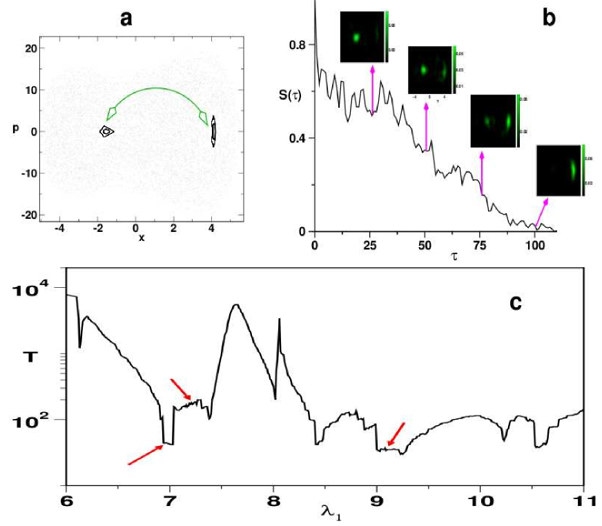
Figure 5: (a) Phase space for the driven double well system with field strength $\lambda_{1}=10$. A coherent state localized in the left regular island tunnels (indicated by a green arrow) over to the right regular island. The chaotic regions (gray) have been suppressed for clarity. (b) Monitoring the survival probability of the initial state to determine the timescale of tunneling ($\sim$ $100\tau$ in this case). Snapshots of the evolving Husimi distributions are also shown at specific intervals, with green (gray) indicating maxima of the distributions. (c) The decay time determined as in (b) for a variety of field strengths with the initial state localized in the left island. Note the fluctuations in the decay time over several orders of magnitude despite very similar nature of the phase spaces over the entire range of the driving field strength. The arrows highlight some of the plateau regions which are crucial for bichromatic control.

In order to illustrate the tunneling process Fig. 5a shows the stroboscopic surface of section for the case of strong driving with $\lambda_{1}=10$. Note the extensive chaos and the two regular islands (left and right) in the phase space. A coherent state $|z\rangle\equiv|x_{0},p_{0}\rangle$ is placed in the center of the left island and time evolved using the Floquet approach which is ideally suited for time-periodic driven systems. In this instance one is interested in the time at which the coherent state localized on the left tunnels over to the regular region on the right. In order to obtain this information it is necessary to compute the survival probability of the initial coherent state. Briefly, Floquet states {$|\chi_{n}\rangle$} are eigenstates of the Hermitian operator $H-i\hbar\partial/\partial t$ and form a complete orthonormal basis. An arbitrary time-evolved state $|z(t)\rangle$ can be expressed as

$$|z(t)\rangle=\sum_{n}A_{n}e^{-iE_{n}t}|\chi_{n}(t)\rangle,$$ (12)

with $E_{n}$ being the quasienergy associated with the Floquet state $|\chi_{n}\rangle$. The expansion coefficients $A_{n}$ are independent of time and given by

$$A_{n}=\langle\chi_{n}(0)|z(0)\rangle,$$ (13)

yielding the expansion

$$|z(t)\rangle=\sum_{n}e^{-iE_{n}t}|\chi_{n}(t)\rangle\langle\chi_{n}(0)|z(0)\rangle.$$ (14)

Measuring time in units of field period ($T_{f}$) and owing to the periodicity of the Floquet states, $|\chi_{n}(t)\rangle=|\chi_{n}(t+T_{f})\rangle$, the above equation simplifies to

$$|z(\tau)\rangle=\sum_{n}e^{-iE_{n}\tau}|\chi_{n}(0)\rangle\langle\chi_{n}(0)|z(0)\rangle\equiv\hat{U}(\tau)|z(0)\rangle,$$ (15)

with $\tau\equiv kT_{f}$ and integer $k$.

The time evolution operator

$$\hat{U}(\tau)=\sum_{n}e^{-iE_{n}\tau}|\chi_{n}(0)\rangle\langle\chi_{n}(0)|,$$ (16)

is determined by successive application of the one-period time evolution operator $U(T_{f},0)$ i.e.,

$$\hat{U}(kT_{f},0)=[\hat{U}(T_{f},0)]^{k}.$$ (17)

This allows us to express the survival probability of the initial coherent state in terms of Floquet states as

$$S(\tau) \equiv |\langle z(0)|z(\tau)\rangle|^{2}$$ (18)

$$= \left|\sum_{n}e^{-iE_{n}\tau}\langle z(0)|\chi_{n}(0)\rangle\langle\chi_{n}(0)|z(0)\rangle\right|^{2}$$

$$= \sum_{m,n}p_{zn}p_{zm}e^{-i(E_{n}-E_{m})\tau},$$

where the overlap intensities are denoted by $p_{zn}\equiv|\langle z(0)|\chi_{n}(0)\rangle|^{2}$. In order to determine the “lifetime” ($T$) of the initial coherent state, we monitor the time at which $S(\tau)$ goes to zero (minimum) at the first instance. In other words, it is the time when the coherent state leaves its initial position i.e, the left regular island of the phase space for the first time. In Fig. 5b the $S(\tau)$ for the initial state of interest is shown along with the snapshots of Husimi distribution at specific times. Clearly, the initial state tunnels in about $100T_{f}$, which suggests that chaos assists the dynamical tunneling process. However, the issue is subtle and highlighted in Fig. 5c which shows the decay time plot for a range of driving field strengths for an intial state localized in the left regular island. It is important to note that the gross features of the phase space are quite similar over the entire range. However, Fig. 5c exhibits strong fluctuations over several orders of magnitude and this implies that a direct association of the decay time with the extent of chaos in the phase space is not entirely correct.

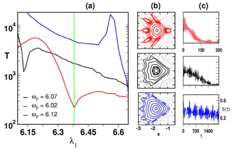
Figure 6: Decay time plot for $\omega_{F}=\omega_{F}^{(0)}\equiv 6.07$ (black) and for $\omega_{F}^{(0)}+0.05$ (blue) and $\omega_{F}^{(0)}-0.05$ (red) as a function of $\lambda_{1}$. The local phase structure in the vicinity of the initial coherent state and the survival probability for fixed $\lambda_{1}=6.4$ (indicated by green line in (a)) corresponding to red shifted, fundamental and blue shifted field frequency is shown in panels (b) and (c) respectively. The $6$:$1$ field-matter resonance in case of $\omega_{F}^{(0)}-0.05$ is clearly visible and correlates with the very short decay time as compared to the other two cases. Note the different time axis scale in the first survival probability plot.

The above discussion and results summarized in Fig. 5 bring up the following key question. What is the mechanism by which the initial state $|z\rangle$ decays out of the regular region? In turn, this is precisely the question that modern theories of dynamical tunneling strive to answer. According to the theory of resonance-assisted tunnelingseu05 ; es05 ; Schl06 , the mechanism is possibily one wherein $|z\rangle$ couples to the chaotic sea via one or several nonlinear resonances provided certain conditions are satisfied. Specifically, the local structure of the phase space surrounding the regular region is expected to play a critical role. The theoretical underpinnings of RAT along with several illuminating examples can be found in the contribution by Schlagheck et al. and here we suggest a simple numerical example which points to the importance of the local phase space structure around $|z\rangle$.

Preliminary evidence for the role of field-matter nonlinear resonances in controlling the decay of $|z\rangle$ is given in Fig. 6, which shows the effect of changing the driving field frequency $\omega_{F}$ on the local phase space structures and the decay times. From Fig. 6 it is apparent that detuning $\omega_{F}$ by $\pm 0.05$ leads to a significant change in the local phase space structure and the decay time of the initially localized state. In Fig. 6(b), corresponding to the field frequency $\omega_{F}=6.02$, a prominent $6$:$1$ field-matter resonance is observed. It is plausible that the the decay time is only a few hundred field periods in this case due to assistance from the nonlinear resonance. However, the decay time increases for $\omega_{F}=6.07$ and becomes even larger by an order of magnitude for $\omega_{F}=6.12$, due to absence of the $6$:$1$ resonance. This indicates that decay dynamics is highly sensitive to the changes in local phase space structure of the left regular island. Therefore, taking into account the relatively large order resonances, since $\hbar=1$, is unavoidable in order to understand the decay time plot in Fig. 5 and for smaller values of the effective Planck constant one expects a more complicated behavior. Note, however that the very high order island chain visible in the last case in Fig. 6 is unable to assist the decay. This is where we believe that an extensive $\hbar$-scaling study will help in gaining a deeper understanding of the decay mechanism. Such an extensive calculation can be found, for example, in the recent workmes06 by Mouchet, Eltschka, and Schlagheck on the driven pendulum. There is sufficient evidencemes06 in the driven pendulum system for a mechanism in which nonlinear resonances play a central role in coupling initial states localized in regular phase space regions to the chaotic sea. One might be able to provide a clear qualitative and quantitative explanation for the results in Fig. 5c based on the recent advances.

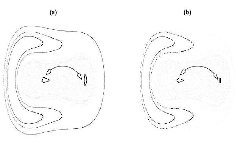
Figure 7: Stroboscopic surface of sections for the bichromatically driven double well system with the control field strength fixed at $\lambda_{2}=0.7$ and primary field strength (a) $\lambda_{1}=9.2$ and (b) $\lambda_{1}=10.0$. As in the earlier plots, the chaotic regions have been suppressed (in gray) for clarity. Note the breaking of the symmetry in both cases. However, significant suppression of the deacy of the state localized in the left regular island happens in case (b) only.

III.1.1 CAT spoils bichromatic control

This brings us to the second important issue - what is the role of chaos in this dynamical tunneling process? An earlier workudh94 by Utermann, Dittrich and Hänggi on the driven double well system showed that there is indeed a strong correlation between the splittings of the Floquet states and the overlaps of their Husimi distributions with the chaotic regions in the phase space. However, a different perspective yields clear insights into the role of chaos with potential implications for coherent control. In order to highlight this perspective I start with a simple question: is it possible to control the decay of the localized initial state with an appropriate choice of a control field? It is important to note that the Lin-Ballentine system parameters imply that one is dealing with a multilevel control scenario and there has been a lot of activity over the last few years to formulate control schemes involving multiple levels in both atomic and molecular systems. The driven double well system has been a particular favorite in this regard, more so in recent times due to increased focus on the physics of trapped Bose-Einstein condensatesmo06 . More specifically, several studies have explored the possibility of controlling various atomic and molecular phenomenon using bichromatic fields with the relative phase between the fields providing an additional control parameter. In the present context, for example, Sangouard et al. exploited the physics of adiabatic passage to show that an appropriate combination of $(\omega_{F},2\omega_{F})$ field leads to suppression of tunneling in the driven double well modelprl04-sgmj-chap2 . The choice of relative phase between the two fields allowed them to localize the initial state in one or the other well. However, the parameter regimes in the work by Sangouard et al. correspond to the underlying phase space being near-integrable and hence a minimal role of the chaotic sea.

More relevant to the mixed regular-chaotic phase space case presented in Fig. 5 is an earlier workfm93 by Farrelly and Milligan wherein it was demonstrated that one can suppress the tunneling dynamics in a driven double well system using a $(\omega_{F},2\omega_{F})$ bichromatic field. In other words the original Hamiltonian of Eq. 10 is modified as following

$$H(x,p;t)=H_{0}(x,p)+\lambda_{1}x\cos(\omega_{F}t)+\lambda_{2}x\cos(2\omega_{F}t+\phi),$$ (19)

with $H_{0}(x,p)$ being the same as in Eq. 11 and the additional $2\omega_{F}$-field is taken to be the control field. Moreover, modulating the turn-on time of the control field can trap the wavepacket in the left or right well of the double well potential. Hence, it was arguedfm93 that the tunneling dynamics in a driven double well can be controlled at will for specific choices of the control field parameters $(\lambda_{2},\phi)$. Note that in the presence of control field i.e., $\lambda_{2}\neq 0$ with the relative phase $\phi=0$ the Hamiltonian in Eq. 19 transforms under symmetry operations as

$$H\left(-x,-p;t+\frac{\pi}{\omega_{F}}\right) = H_{0}(x,p)-x[\lambda_{1}\cos(\omega_{F}t+\pi)+\lambda_{2}\cos(2\omega_{F}t+2\pi)]$$

$$= H_{0}(x,p)-x[-\lambda_{1}\cos(\omega_{F}t)+\lambda_{2}\cos(2\omega_{F}t)]$$

$$\neq H(x,p;t).$$

Similarly, except at $\phi=\pi/2$, the discrete symmetry of the Hamiltonian is broken under the influence of the additional $2\omega_{F}$-field. Farrelly and Milligan thus arguedfm93 that the control field with strength smaller than the driving field will lead to localization due to the breaking of the generalized symmetry of the Hamiltonian and the Floquet states. The impact of a small symmetry breaking control field with $(\lambda_{2},\phi)=(0.7,0)$ can be clearly seen in Fig. 7 in terms of the changes in the classical phase space structures. However, there is a subtlety which is not obvious upon inspecting the phase spaces shown in Fig. 7 for two different but close values of the driving field strength. In case of $\lambda_{1}=9.2$ corresponding to Fig. 7(a), the control field is unable to suppress the decay of the initial state $|z\rangle$ localized in the left regular region. On the other hand, Fig. 7(b) corresponds to $\lambda_{1}=10$ and computations show that the control field is able to suppress the decay of $|z\rangle$ to an appreciable extent. Thus, although in both cases the control field breaks the symmetry and the resulting phase spaces show very similar structures, the extent of control exerted by the $2\omega_{F}$-field is drastically different.

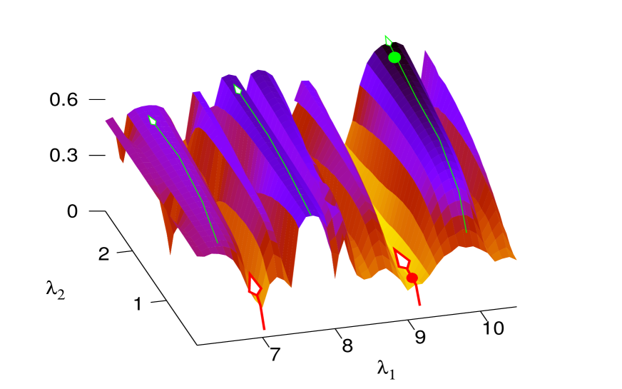
Figure 8: Time-smoothed survival probability representation of the control landscape for $\phi=0$ as a function of the field parameters $(\lambda_{1},\lambda_{2})$. The initial state in every case is localized in the left regular region in the classical phase space. Notice the convoluted form of the landscape with the regions of low probability indicating little to no control (red thick arrows). The green lines (thin arrows) indicate regions where a high degree of control can be achieved.

The discussions above and the results summarized in Fig. 7 and Fig. 6 clearly indicate that the decay of $|z\rangle$ out of the left regular region can be very different and deserves to be understood in greater detail. In fact, computations show that such cases of complete lack of control are present for other values of $\lambda_{1}$ as well. This is confirmed by inspecting Fig. 8 which shows the control landscape for the bichromatically driven double well in the specific case of $\phi=0$. Other choices for $\phi$ also show similarly convoluted landscapes. There are several ways of presenting a control landscape and in Fig. 8 the time-smoothed survival probability (cf. Eq. 18)

$$\langle S\rangle=\frac{1}{\tau}\int_{0}^{\tau}d\tau^{\prime}S(\tau^{\prime})$$ (21)

associated with the initial state $|z\rangle$ is used to map the landscape as a function of the field strengths $(\lambda_{1},\lambda_{2})$. Note that the choice of $\langle S\rangle$ to represent the landscape is made for convenience; the decay time is a better choice which requires considerable effort but the gross qualitative features of the control landscape do not change upon using $\langle S\rangle$. Large (small) values of $\langle S\rangle$ indicate that the decay dynamics is suppressed (enhanced). It is clear from Fig. 8 that the landscape comprises of regions of control interspersed with regions exhibiting lack of control. Such highly convoluted features of control landscape are a consequence of the simple bichromatic choice for the control field and the nonlinear nature of the corresponding classical dynamics. From a control point of view, there are regions on the landscape for which a monotonic increase of $\lambda_{2}$ leads to increasing control. Interestingly, the lone example of control illustrated in Farrelly and Milligan’s paperfm93 happens to be located on one of the prominent hills on the control landscape (shown as a green dot in Fig. 8). A striking feature that can be seen in Fig. 8 is the deep valley around $\lambda_{1}=9.2$ which signals an almost complete lack of control even for significantly large strengths of the $2\omega_{F}$-field. The valleys in Fig. 8 correspond precisely to the plateaus seen in the decay time plot shown in Fig. 6 for $\lambda_{2}=0$ (red arrows). It is crucial to note that this “wall of no control” is robust even upon varying the relative phase $\phi$ between the driving and the control field.

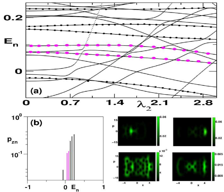
Figure 9: (a) Variation of the Floquet quasienergies with $\lambda_{2}$. The primary driving field strength is fixed at $\lambda_{1}=9.2$. Six states that have appreciable overlap with $|z\rangle$ are highlighted by circles. (b) Overlap intensity $p_{zn}$ for $\lambda_{1}=9.2$ and $\lambda_{2}=2.1$ indicates multilevel interactions involving the states shown in (a). Husimi distribution function of the Floquet states regulating the decay of $|z\rangle$ are also shown. Notice that the nature of delocalized states (magenta) does not change much with $\lambda_{2}$.

Insights into the lack of control for driving field strength $\lambda_{1}=9.2$ (and other values as well which are not discussed here) can be obtained by studying the variation of the Floquet quasienergies with $\lambda_{2}$, the control field strength. In Fig. 9 the results of such a computation are shown and it is immediately clear that even in the presence of $2\omega_{F}$-control field six states contribute to the decay of $|z\rangle$ over the entire range of $\lambda_{2}$. This is further confirmed in Fig. 9(b) where the plot of the overlap intensities shows multiple Floquet states participating nearly equally in the decay dynamics of the initial state. The final clue comes from inspecting the Husimi distributions shown in Fig. 9, highlighting the phase space delocalized nature of some of the participating states. Despite the symmetry of the tunneling doublets being broken due to the bichromatic field, two or more of the participating states are extensively delocalized in the chaotic reigons of the phase space. Moreover, the participation of the chaotic Floquet states persists even for larger values of $\lambda_{2}$. Hence, using the symmetry breaking property of the $2\omega_{F}$-field for control purposes is not very effective when chaotic states are participating in the dynamics. Therefore, the lack of control, signaled by plateaus in Fig. 6 and the valleys in Fig. 8, is due to the dominant participation by chaotic states i.e., chaos-assisted tunneling. The plateaus arise due to the fact that the coupling between the localized states and the delocalized states vary very little with increasing control field strength $\lambda_{2}$ - something that is evident from the Floquet level motions shown in Fig. 9 and established earlier by Tomsovic and Ullmo in their seminal work on chaos-assisted tunneling in coupled quartic oscillatorstu94 . It is important to note that for $\lambda_{2}=0$ the chaotic states, as opposed to the regular states, do not have a definite parity. Consequently, the presence of the $2\omega_{F}$-field does not have a major influence on the chaotic states. Thus, if one or more chaotic states are already influencing the dynamics of $|z\rangle$ at $\lambda_{2}=0$ then the bichromatic control is expected to be difficult. An earlier studylgw94 by Latka et al. on the bichromatically driven pendulum system also suggested that the ability to control the dynamics is strongly linked to the existence of chaotic states.

The model problem in this section and the results point to a direct role of chaos-assisted pathways in the failure of an attempt to bichromatically control the dynamics. However, it is not yet clear if control strategies involving more general fields would exhibit similar characteristics. There is some evidence in the literature which indicates that quantum optimal control landscapes might be highly convoluted if the underlying classical phase space exhibits large scale chaossr91 . Nevertheless, further studies need to be done and the resulting insights are expected to be crucial in any effort to control the dynamics of multilevel systems.

III.2 Driven Morse oscillator: resonance-assisted tunneling

The driven Morse oscillator system has served as a paradigm model for understanding the dissociation dynamics of diatomic molecules. Studies spanning nearly three decades have explored the physics of this system in exquisite detail. Consequently, a great deal is known about the mechanism of dissociation both from the quantum and classical perspectives. Indeed, the focus of researchers nowadays is to control, either suppress or enhance, the dissociation dynamics and various suggestions have been put forward. In addition, one hopes that the ability to control a single vibrational mode dynamics can lead to a better understanding of the complications that arise in the case of polyatomic molecular systems wherein several vibrational modes are coupled at the energies of interest.

Several important insights have originated from classical-quantum correspondence studies which have established that molecular dissociation, in analogy to multiphoton ionization of atoms, occurs due to the system gaining energy by diffusing through the chaotic regions of the phase space. For example, an important experimental study by Dietrich and Corkum has shownjcp92-dc-chap3 , amongst other things, the validity of the chaotic dissociation mechanism. Thus, the formation of the chaotic regions due to the overlappr79-ch-chap3 of nonlinear resonances (field-matter), hierarchical structuresprl84-mmp-chap3 near the regular-chaotic borders acting as partial barriers, and their effects on quantum transportprl88-rp-chap3 have been studied in a series of elegant papersbw861 ; pra87-gy-chap3 ; pra91-gh-chap3 . In the context of this present article an interesting question is as follows. Since a detailed mechanistic understanding of the role of various phase space structures of the driven Morse system is known, is it possible to design local phase space barriers to effect control over the dissociation dynamics? In particular, the central question here is whether the local phase space barriers are also able to suppress the quantum dissociation dynamics. There is an obvious connection between the above question and the theme of this volume - quantum mechanics can “shortcircuit” the classical phase space barriers due to the phenomenon of dynamical tunneling. Thus, such phase space barriers might be very effective in controlling the classical dissociation dynamics but might fail completely when it comes to controlling the quantum dissociation dynamics. There is a catch here, however, since there is also the possibility that the cantori barrier in the classical phase space may be even more restrictive in the quantum case. Thus, creation or existence of a phase space barrier invariably leads to subtle competition between classical transport and quantum dynamical tunneling through the barrier. As expected, the delicate balance between the classical and quantum mechanism is determined by the effective Planck constant of the system of interest. An earlier detailed reviewgrr86 by Radons, Geisel and Rubner is highly reccomended for a nice introduction to the subject of classical-quantum correspondence perspective on phase space transport through Kolmogoroff-Arnol’d-Moser (KAM) and cantori barriers. In the driven Morse oscillator case, Brown and Wyatt showedbw861 that the cantori barriers do leave their imprint on the quantum dissociation dynamics and act as even stronger barriers as compared to the classical system. Maitra and Heller in their studypre00-mh-chap3 on transport through cantori in the whisker map have clearly highlighted the classical versus quantum competition.

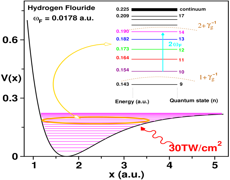
Figure 10: A plot of Morse potential along with the bound states supported by the potential well. A schematic view of energy level diagram for Morse eigenstates under study in this chapter is shown as inset. The laser field of intensity $\lambda_{1}=0.0287$ and frequency $\omega_{F}=0.0178$ connects state $n=10$ and $n=14$ via a two-photon resonance transition. The location of cantori in presence of the field with $\omega_{F}=0.0178$ are indicated as dotted curves in the figure.

From the above discussion it is apparent that any approach to control the dissociation dynamics by recreating local phase space barriers will face the subtle classical-quantum competition. In fact, it is tempting to think that every quantum control algorithm works by creating local phase space dynamical barriers and the efficiency of the control is decided by the classical-quantum competition. However, at this point of time there is very little work towards making such a connection and the above statement is, at best, a conjecture. For the purpose of this article, I turn to the driven Morse oscillator system to provide an example for the importance of resonance-assisted tunneling in controlling the dissociation dynamics.

The model system is inspired from the early workbw861 by Wyatt and Brown (see also the work by Breuer and Holthausbh93 ) and the Hamiltonian can be written as

$$H(x,p;t)=H_{0}(x,p)-\mu(x)\lambda_{1}\cos(\omega_{F}t),$$ (22)

in the dipole approximation. The zeroth-order Hamiltonian

$$H_{0}(x,p)=\frac{1}{2M}p^{2}+D_{0}{[1-e^{{-\alpha(x-x_{e})}}]}^{2},$$ (23)

represents the Morse oscillator modeling the anharmonic vibrations of a diatomic molecule. In the above, $\mu(x)$ is the dipole moment function, $\lambda_{1}$ is the strength of the laser field, $\omega_{F}$ is the driving field frequency, and

$$M=\frac{m_{1}m_{2}}{m_{1}+m_{2}},$$ (24)

is the reduced mass of the diatomic molecule with $m_{1}$ and $m_{2}$ being the two atomic masses. In Eq. 23, $D_{0}$ is the dissociation energy, $\alpha$ is the range of the potential and $x_{e}$ is the equilibrium bond length of the molecule.

Rather than attempting to provide a general account as to how RAT might interfere with the process of control, I feel that it is best to illustrate with a realistic molecular example. Hopefully, the generality of the arguments will become apparent later on. For the present purpose I choose the diatomic molecule hydrogen fluoride (HF) as the specific example. Any diatomic molecule could have been chosen but HF is studied here due to the fact that Brown and Wyatt have already discussed the role of cantori barriers to the dissociation dynamics in some detail. The Morse oscillator parameters for hydrogen fluoride are $D_{0}=0.225,\alpha=1.174,x_{e}=1.7329$ and $M=1744.59$. These parameters correspond to ground electronic state of the HF molecule supporting $N_{B}=24$ bound states. Note that atomic units are used for both the molecular and field parameters with time being measured in units of the field period $\tau_{F}=2\pi/\omega_{F}$. The only difference between the present work and that of Brown and Wyatt has to do with the field-matter coupling. Brown and Wyatt use the dipole function

$$\mu(x)=Axe^{-B{x^{4}}},$$ (25)

with $A=0.4541$ and $B=0.0064$, obtained from ab-initio data on HF. Here a linear approximation for $\mu(x)$

$$\mu(x) \approx \mu(x_{e})+\left(\frac{\partial\mu}{\partial x}\right)_{x_{e}}(x-x_{e})$$ (26)

$$\equiv \mu(x_{e})+d_{1}(x-x_{e}),$$

is employed with $d_{1}\approx 0.33$ in case of HF. There are quantitative differences in the dissociation probabilities due to the linearization approximation but the main qualitative features remain intact despite the linearization approximation.

In Fig. 10 the Morse potential for HF is shown along with a summary of the key features such as the energy region of interest, the quantum state whose dissociation is to be controlled, and the classical phase space structures that might play an important role in the dissociation dynamics. The driving field parameters are chosen as $(\omega_{F},\lambda_{1})=(0.0178,0.0287)$, same as in the earlier workbw861 , and the field strength corresponds to about $30$ TW/cm${}^{2}\equiv 30\times 10^{12}$ W/cm². As shown in Fig. 10 (inset), the focus is on understanding and controlling the dissociation dynamics of the $n=10$ excited Morse oscillator eigenstate. There are several reasons for such a choice and I mention two of the most important reasons. Firstly, the earlier studybw861 has established that $n=10$ of HF happens to be in an energy regime wherein two specific cantori barriers in the classical phase space affect the dissociation dynamics. Moreover, for driving frequency $\omega_{F}=0.0178$, two of the zeroth-order eigenstates $n=10$ and $n=14$ have unperturbed energies such that $E_{14}-E_{10}\approx 2\hbar\omega_{F}$ and hence corresponds to a two-photon resonant situation. Secondly, for a field strength of $30$ TW/cm², the dissociation probability of the ground vibrational state is negligible. Far stronger field strengths are required to dissociate the $n=0$ state and ionization process starts to compete with the dissociation at such high intensities. Thus, in order to to illustrate the role of phase space barriers in the dissociation dynamics without such additional complications, the specific initial state $n=10$ is chosen. Incidentally, such a scenario is quite feasible since a suitably chirped laser field can populate the $n=10$ state very efficiently from the initial ground state $n=0$ and one imagines coming in with the monochromatic laser to dissociate the molecule.

III.2.1 Nature of the classical phase space

The monochromatically driven Morse system studied here has a dimensionality such that one can conveniently visualize the phase space in the original cartesian $(x,p)$ variables. However, since the focus is on suppressing dissociation by creating robust KAM tori in the phase space, action-angle variables $(J,\theta)$ which are canonically conjugate to $(x,p)$ are convenient and a natural representation to work with. The action-angle variables $(J,\theta)$ of the unperturbed Morse oscillator, appropriate for the bound regions, are given byrm71

$$J = \sqrt{\frac{2MD_{0}}{\alpha^{2}}}\left(1-\sqrt{1-E}\right)$$ (27a)

$$\theta = -sgn(p)\cos^{-1}\left[\frac{1-E}{\sqrt{E}}e^{\alpha(x-x_{e})}-\frac{1}{\sqrt{E}}\right].$$ (27b)

In the above equations, $E=H_{0}/D_{0}<1$ denotes the dimensionless bound state energy, and $sgn(p)=1$ for $p\geq 0$, $sgn(p)=-1$ for $p<0$. In terms of the action-angle variables it is possible to express the cartesian $(x,p)$ as follows

$$x = x_{e}+\frac{1}{\alpha}\ln\left[\frac{1+\sqrt{E_{0}(J)}\cos\theta}{(1-E_{0}(J))}\right]$$ (28a)

$$p = \frac{-(2MD_{0})^{1/2}[E_{0}(J)(1-E_{0}(J))]^{1/2}\sin\theta}{1+\sqrt{E_{0}(J)}\cos\theta},$$ (28b)

where $E_{0}(J)=H_{0}(J)/D_{0}$. Substituting for $(x,p)$ in terms of $(J,\theta)$, the unperturbed Morse oscillator Hamiltonian in Eq. 23 is transformed into

$$H_{0}(J)=\omega_{0}\left(J-\frac{\omega_{0}}{4D_{0}}J^{2}\right),$$ (29)

where $\omega_{0}=\sqrt{2\alpha^{2}D_{0}/M}$ is the harmonic frequency at the minimum. The zeroth-order nonlinear frequency is easily obtained as

$$\Omega_{0}(J)\equiv\frac{\partial H_{0}}{\partial J}=\omega_{0}\left(1-\frac{\omega_{0}}{2D_{0}}J\right),$$ (30)

and with increasing excitation i.e., increasing action (quanta) $J$, the non-linear frequency $\Omega_{0}(J)$ decreases monotonically and eventually vanishes, signaling the onset of unbound dynamics leading to dissociation.

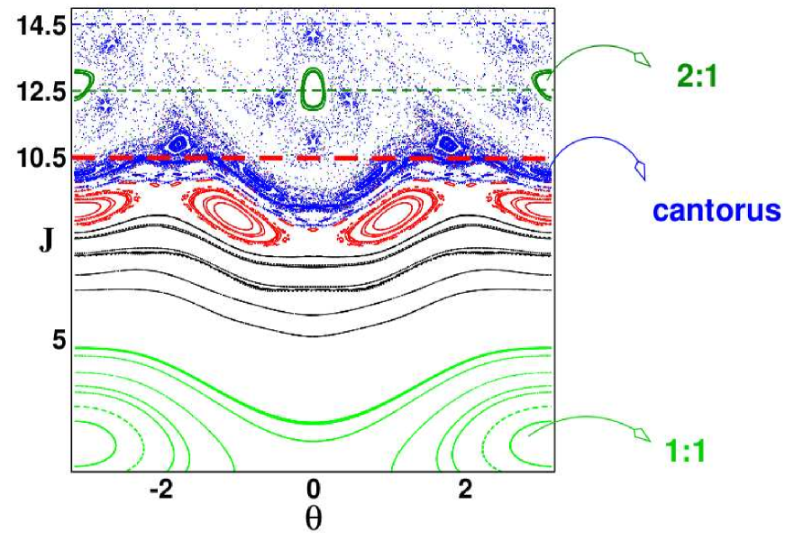
Figure 11: The phase space, as a stroboscopic surface of section, for the driven Morse system with laser field of intensity $\lambda_{1}=0.0287$ and frequency $\omega_{F}=0.0178$ corresponding to a on-resonance situation. The $2$-photon resonance is clearly seen in the phase space and marked as $2$:$1$ resonance in dark green. The initial Morse eigenstate $n=10$ (thick dashed line) is situated rather close to a cantorus (indicated), $\omega_{F}/\Omega_{0}(J)=1+\gamma_{g}^{-1}$ with $\gamma_{g}\equiv(1+\sqrt{5})/2$ being the golden ratio. The $n=10$ state is connected to the $n=14$ Morse eigenstate via the $2$:$1$ resonance. Note that the states $n=10,12$, and $14$ are symmetrically located about the resonance with $n=12$ being localized in the resonance.

The driven system can now be expressed in terms of the variables $(J,\theta)$ as

$$H(J,\theta;t)=H_{0}(J)-\frac{\epsilon}{\alpha}\ln\left[\frac{1+\sqrt{E_{0}(J)}\cos\theta}{(1-E_{0}(J))}\right]\cos(\omega_{F}t).$$ (31)

In addition, since $x$ is a periodic function of $\theta$, one has the Fourier expansion

$$x=2\left[V_{0}(J)+\sum_{n=1}^{\infty}V_{n}(J)\cos(n\theta)\right].$$ (32)

As a consequence the driven Hamiltonian in Eq. 31 can be written as

$$H(J,\theta;t)=H_{0}(J)-\epsilon v(J,\theta;t),$$ (33)

where the matter-field interaction term is denoted as

$$v(J,\theta;t)=2\left[V_{0}(J)+\sum_{n=1}^{\infty}V_{n}(J)\cos(n\theta)\right]\cos(\omega_{F}t),$$

The Fourier coefficients $V_{0}(J)$ and $V_{n}(J)$ are known analytically and given by

$$V_{0}(J) = \frac{1}{2\alpha}\ln\left[\frac{D_{0}+\sqrt{{D_{0}}^{2}-D_{0}E_{0}(J)}}{2(D_{0}-E_{0}(J))}\right],$$ (34a)

$$V_{n}(J) = \frac{(-1)^{n+1}}{\alpha n}{\left[\frac{\sqrt{D_{0}E_{0}(J)}}{D_{0}+\sqrt{D_{0}^{2}-D_{0}E_{0}(J)}}\right]}^{n}.$$ (34b)

The stroboscopic surface of section in the $(J,\theta)$ variables is shown in Fig. 11 and is a typical mixed regular-chaotic phase space. A few important points are worth noting at this stage. Firstly, the initial state of interest is located close to a cantorus with $\omega_{F}:\Omega_{0}(J)=1+\gamma_{g}^{-1}$ with $\gamma_{g}\equiv(1+\sqrt{5})/2$ being the golden ratio. The importance of this cantorus to the resulting dissociation dynamics of the $n=10$ state was the central focus of the work by Brown and Wyattbw861 . In particular, the extensive stickiness around this region can be clearly seen and hence one expects nontrivial influence on the classical dissociation dynamics as well. Secondly, a prominent $\omega_{F}$:$\Omega_{0}(J)=2$:$1$ nonlinear resonance is also observed in the phase space and represents the classical analog of the quantum $2$-photon resonance condition. Interestingly, the area of this resonance is about $\hbar$ and, therefore, can support one quantum state. It turns out that the Husimi density of the Morse state $n=12$ is localized inside the $2$:$1$ resonance island. In addition, the states $n=10$ and $n=14$ are nearly symmetrically located about the $2$:$1$ resonance. A way to see this is to use secular pertubation theory on the driven Morse Hamiltonian. One can show that in the vicinity of the $2$:$1$ resonance (cf. Fig. 11) an effective pendulum Hamiltonian

$$H_{eff}(J,\phi)\simeq\frac{1}{2\tilde{m}_{2:1}}{(\Delta J)}^{2}+2\tilde{V}_{2:1}(J_{2:1})\cos(2\phi),$$ (35)

is obtained with $\Delta J=J-J_{2:1}$, $\tilde{m}_{2:1}=2D_{0}/\omega_{0}^{2}$ and $V_{2:1}(J)=\epsilon V_{1}(J)/2$. The resonant action

$$J_{2:1}=\frac{2D_{0}}{\omega_{0}}\left[1-\frac{\omega_{F}}{2\omega_{0}}\right]\approx 12.6,$$ (36)

for the parameters used in this work. Using action values $J=10.5$ (quantum state $n=10$) and $J^{\prime}=14.5$ (quantum state $n^{\prime}=14$) the energy difference is calculated as

$$|E_{J}-E_{J^{\prime}}| = \left|\frac{1}{2\tilde{m}_{2:1}}(J-J^{\prime})(J+J^{\prime}-2J_{2:1})\right|$$

$$\approx 3.2\times 10^{-4}\ll E_{J}.$$

In other words, the states $n=10$ and $n=14$ are nearly symmetrical with respect to the state $n=12$, which is localized in the $2$:$1$ resonance. Therefore, the nonzero coupling $V_{2:1}$ will efficiently connect the states $n=10$ and $n=14$. Moreover, for the given parameters, using the definition of $V_{r:s}(J)$ in terms of Fourier coefficient $V_{1}$, the strength of the resonance is estimated as $V_{2:1}(J_{2:1})\approx 0.01464$, clearly a fairly strong resonance. Consequently, the situation in Fig. 11 is a perfect example where RAT can play a crucial role in the dissociation dynamics. Indeed quantum computations (not shown here) show that there is a Rabi-type cycling of the probabilities between the three Morse states. I now turn to the issue of selectively controlling the dissociation dynamics of the initial Morse eigenstate $n=10$ by creating local barriers in the phase space shown in Fig. 11, bearing in mind the possibility of quantum dynamical tunneling interfering with the control process.

III.2.2 Creating a local phase space barrier

If the classical mechanism of chaotic diffusion leading to dissociation holds in the quantum domain as well then a simple way of controlling the dissociation is to create a local phase space barrier between the state of interest and the chaotic region. In a recent workchandre , Huang, Chandre and Uzer provided the theory for recreating local phase space barriers for time-dependent systems and showed that such barriers indeed suppress the ionization of a driven atomic system. However, Huang et al. were only concerned with the classical ionization process. Thus, potential complications due to dynamical tunneling were not addressed in their study. The driven Morse system studied here presents an ideal system to understand the interplay of quantum and classical dissociation mechanisms. In what follows, I provide a brief introduction to the methodology with an explicit expression for the classical control field needed to recreate an invariant KAM barrier, preferably an invariant torus with sufficiently irrational frequency $\Omega_{r}$.

To start with, the nonautonomous Hamiltonian is mapped into an autonomous one by considering $(t({\rm mod}2\pi),E)$ as an additional angle-action pair. Denoting the action and angle variables by ${\bf A}\equiv(J,E)$ and ${\bm{\theta}}\equiv(\theta,t)$, the original driven system Hamiltonian (see Eq. 33) can be expressed as

$$H({\bf A},{\bm{\theta}})=H_{0}({\bf A})-\epsilon V({\bf A},{\bm{\theta}}),$$ (38)

with $V({\bf A},{\bm{\theta}})\equiv v(J,\theta;t)$. Note that for a fixed driving field strength $\lambda_{1}$ and the value of $d_{1}$ corresponding to a diatomic molecule, $\epsilon\equiv\lambda_{1}d_{1}$ is also fixed. Moreover, for physically meaningful values of $d_{1}$ for most diatoms and typical field strengths far below the ionization threshold one always has $\epsilon\ll 1$. In the absence of the driving field ($\epsilon=0$), the zeroth-order Hamiltonian is integrable and the phase space is foliated with invariant tori labeled by the action ${\bf A}$ corresponding to the frequency ${\bm{\omega}}\equiv\partial H_{0}/\partial{\bf A}=(\Omega_{0},\omega_{F})$. However, in the presence of the driving field ($\epsilon\neq 0$) the field-matter interaction renders the system nonintegrable with a mixed regular-chaotic phase space. More specifically, for field strengths near or above a critical value $\epsilon_{c}$ one generally observes a large scale destruction of the field-free invariant tori leading to significant chaos and hence the onset of dissociation. The critical value $\epsilon_{c}$ itself is clearly dependent on the specific molecule and the initial state of interest. The aim of the local control method is to rebuild a nonresonant torus ${\bf A}_{0}=(J_{0},0)$, ${\bf k}\cdot{\bm{\omega}}\neq 0$ with integer ${\bf k}$, which has been destroyed due to the interaction with the field. Assuming that the destruction of ${\bf A}_{0}$ is responsible for the significant dissociation observed for some initial state of interest, the hope is that locally recreating the ${\bf A}_{0}$ will suppress the dissociation i.e., ${\bf A}_{0}$ acts as a local barrier to dissociation. Ideally, one would like to recreate the local barrier by using a second field (appropriately called as the control field) which is much weaker and distinct from the primary driving field.

Following Huangchandre et al. such a control field $f({\bm{\theta}})$ can be analytically derived and has the form

$$f({\bm{\theta}})=-H({\bf A}_{0}-\partial_{\bm{\theta}}\Gamma b({\bm{\theta}}),{\bm{\theta}}),$$ (39)

where $b({\bm{\theta}})\equiv H({\bf A}_{0},{\bm{\theta}})=\sum_{{\bf k}}b_{{\bf k}}e^{i{\bf k}\cdot{\bm{\theta}}}$ and $\Gamma$ being a linear operator defined by

$$\Gamma b({\bm{\theta}})\equiv\sum_{{\bf k}\cdot{\bm{\omega}}\neq 0}\frac{b_{\bf k}}{i{\bf k}\cdot{\bm{\omega}}}e^{i{\bf k}\cdot{\bm{\theta}}}.$$ (40)

The classical control Hamiltonian can now be written down as

$$H_{c}({\bf A},{\bm{\theta}}) = H({\bf A},{\bm{\theta}})+f({\bm{\theta}})$$ (41)

$$\equiv H_{0}({\bf A})-\epsilon V({\bf A},{\bm{\theta}})+f({\bm{\theta}}).$$

In case of the driven Morse system the control field can be obtained analytically and to leading order is given by

$$H_{c}(J,\theta;t)\approx H_{0}(J)-\epsilon v(J,\theta;t)+\epsilon^{2}g_{a}(\theta,t),$$ (42)

where

$$g_{a}(\theta,t)=\frac{{\omega_{0}}^{2}}{4D_{0}}{(\partial_{\theta}\Gamma b)}^{2}-2V_{01}(\partial_{\theta}\Gamma b)\cos(\omega_{F}t)-(\partial_{\theta}\Gamma b)\zeta(J,\theta;t),$$ (43)

and it can be shown that

$$V_{01} = \frac{{\omega_{0}}^{2}}{8\alpha\Omega_{r}D_{0}}\left(\frac{2\omega_{0}+\Omega_{r}}{\omega_{0}+\Omega_{r}}\right),$$

$$V_{n1} = (-1)^{n+1}\left(\frac{{\omega_{0}}^{3}}{2\alpha D_{0}}\right)\frac{{(\omega_{0}-\Omega_{r})}^{{\frac{n}{2}}-1}}{{(\omega_{0}+\Omega_{r})}^{\frac{n}{2}+1}},$$ (44)

$$\zeta(J,\theta;t) = \sum_{n=1}^{\infty}V_{n1}(J_{r})[(\cos(n\theta+{\omega}_{F}t)+\cos(n\theta-{\omega}_{F}t)].$$

I skip the somewhat tedious derivation of the result above and refer to the original literaturechandre as well as a recent thesisasthesis for details. Note that in the above $\Omega_{r}$ is the frequency of the invariant torus that is to be recreated corresponding to the unperturbed action

$$J_{r}=(\omega_{0}-\Omega_{r})\frac{2D_{0}}{\omega_{0}^{2}},$$ (45)

and to $O(\epsilon)$ is located at $J(\bm{\theta})=J_{r}-\epsilon\partial_{\theta}\Gamma b$, assuming the validity of the perturbative treatment.

The leading order control field in Eq. 43 is typically weaker than the driving field and has been shownasthesis to be quite effective in off-resonant cases in suppressing the classical dissociation. However, in order to study the effect of the control field on the quantum dissociation probabilities, it is necessary to make some simplifications. One of the main reasons for employing the simplified control fields via the procedure given below has to do with the fact that the classical action-angle variables do not have a direct quantum counterpartcarru68 . Essentially, the dominant Fourier modes $F_{k_{1},k_{2}}$ of Eq. 43 are identified and one performs the mapping

$$F_{k_{1},k_{2}}\cos(k_{1}\theta+k_{2}\omega_{F}t)\rightarrow\lambda_{2}(k_{1},k_{2})\cos(k_{2}\omega_{F}t),$$ (46)

yielding the simplified control Hamiltonian

$$H_{c}=H(J,\theta;t)+\mu(x)\lambda_{2}(k_{1},k_{2})\cos(k_{2}\omega_{F}t).$$ (47)

If more than one dominant Fourier modes are present then they will appear as additional terms in Equation 47. Note that the above simplified form is equivalent to assuming that the control field is polychromatic in nature, which need not be true in general. Nevertheless, a qualitative understanding of the role of the various Fourier modes towards local phase space control is still obtained. More importantly, and as shown next, in the on-resonant case of interest here, the simplified control field already suggests the central role played by RAT.

III.2.3 RAT spoils local phase space control

In Fig. 12 a summary of the efforts to control the dissociation of the initial $n=10$ state is shown. Specifically, Fig. 12(a) and (b) show the phase spaces where two different KAM barriers, $\omega_{F}/\Omega_{r}=1+\gamma_{g}^{-1}$ and $\omega_{F}/\Omega_{r}=\sqrt{3}$ respectively are recreated. The control Hamiltonian in both instances, in cartesian variables, has the following form

$$H_{c}=H_{0}(x,p)-\lambda_{1}\mu(x)\cos(\omega_{F}t)+\lambda_{2}\mu(x)\cos(2\omega_{F}t),$$ (48)

with $\lambda_{2}\approx 0.01\equiv 3$ TW/cm^-2. Thus, as desired, the control field strengths are an order of magnitude smaller than the driving field strength. The simplified control Hamiltonian reflects the dominance of the $F_{3,-2}$ Fourier mode of the leading order control field in Eq. 43 and obtained using the method outlined before. Also, note that the control field comes with a relative phase $\phi=\pi$ with respect to the driving field. As expected, from the line of thinking presented in the previous section, Fig. 12(c) and (d) show that the KAM barriers indeed suppress the classical dissociation significantly. However, the quantum dissociation in both cases increases slightly! Clearly, the recreated KAM barriers are ineffective and suggests that the quantum dissociation mechanism is somehow bypassing the KAM barriers.

A clue to the surprising quantum results comes from comparing the phase spaces in Fig. 11 and Fig. 12 which show the uncontrolled and controlled cases respectively. Although, the KAM barriers seem to have reduced the extent of stochasticity, the $2$:$1$ resonance is intact and appears to occupy slightly larger area in the phase space. Thus, this certainly indicates that a significant amount of the quantum dissociation is occuring due to the RAT mechanism involving the three Morse states $n=10,12$, and $14$ as discussed before. In particular, the $n=12$ state must still be actively providing a route to couple the initial state to the chaotic region via RAT. How can one test the veracity of such an explanation? One way is to scale the Planck constant down from $\hbar=1$ and monitor the quantum dissociation process. Reduced $\hbar$ implies that the $2$:$1$ island can support several states as well as the fact that other higher order resonances now become relevant to the RAT mechanism. Such a study is not presented here but one would anticipate that the dissociation mechanism can be understood based on the theory of RAT that already exists (See contributions by Schlagheck et al. and Bäcker et al., for example). Another way is to directly interfere locally with the resonance and see if the quantum dissociation is actually suppressed. Locally interfering with a specific phase space structure, keeping the gross features unchanged, is not necessarily a straightforward approach. However, the tools in the previous section allow for such local interference and I present the results below.

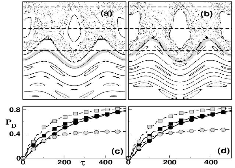
Figure 12: Phase space for the driven Morse system in the presence of the simplified classical control fields (cf. Eq. 47 with $\lambda_{2}\approx 0.01$) designed to recreate specific KAM barriers (a) $\omega_{F}/\Omega_{r}=1+\gamma_{g}^{-1}$ and (b) $\omega_{F}/\Omega_{r}=\sqrt{3}$. Note that in both cases the dominant $F_{3,-2}$ Fourier amplitude of the leading order control field of Eq. 43 have been utilized and the desired KAM barriers are clearly seen (thick gray). The effect of the barriers seen in (a) and (b) on the classical (gray circles) and quantum (gray squares) dissociation probabilities are shown in (c) and (d) respectively. The uncontrolled results are indicated by the corresponding black symbols. Interstingly, the classical dissociation is suppressed but the quantum dissociation is slightly enhanced.

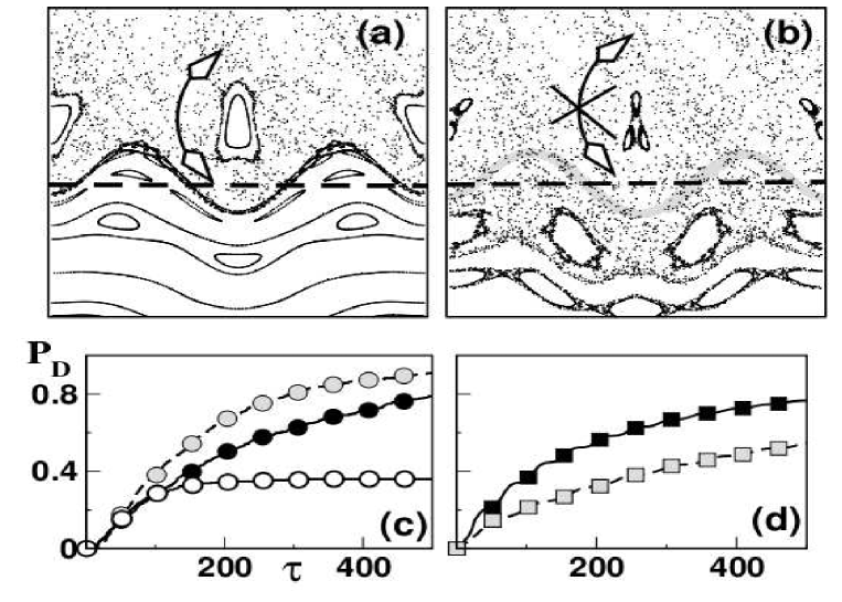
Figure 13: Phase space for the driven Morse system in the presence of the classical control fields designed to recreate the $\omega_{F}/\Omega_{r}=\sqrt{3}$ KAM barrier. In (a) two dominant Fourier modes $F_{3,-2}$ and $F_{4,-2}$ of the leading order control term in Eq. 43 are retained. In (b) the simplified control field as in Eq. 47 is used with an effective field strength estimated using $F_{3,-2}$ and $F_{4,-2}$. Notice that the desired KAM barrier is recreated in (a) but not in (b) (thick gray line indicates the expected location). In (c) the classical dissociation probabilities of the uncontrolled (black circles), control using field (a) (open circles), and control using field (b) (gray circles) are shown. The quantum results are shown in (d) for the uncontrolled (black squares) and control using field (b) (gray squares) are shown. See text for discussion.

The control field in Eq. 43 corresponding to the case of Fig. 12(b) i.e., recreating the $\omega_{F}/\Omega_{r}=\sqrt{3}$ KAM barrier, turns out to be well approximated by

$$H_{c}(J,\theta,t)\approx H(J,\theta,t)+\sum_{n=3,4}F_{n,-2}\cos(n\theta-2\omega_{F}t),$$ (49)

The above Hamiltonian comes about due to the factasthesis that two Fourier modes $F_{3,-2}$ and $F_{4,-2}$ are significant in this case. Note that the specific KAM barrier of interest has a frequency between that of the $1+\gamma_{g}^{-1}$ cantorus (around which the initial state is localized, cf. Fig. 11) and the $2$:$1$ nonlinear resonance. From a perturbative viewpoint, creation of this KAM barrier using Eq. 49 is not expected to be easy due to the proximity to the $2$:$1$ resonance and the fact that the $F_{4,-2}$ Fourier component is nothing but the $2$:$1$ resonance. Nevertheless, Fig. 13(a) shows that the specific KAM barrier is restored and, compared to Fig. 11, the controlled phase space does exhibit reduced amount of chaos. Consisitently, Fig. 13(c) shows that the classical dissociation is suppressed by nearly a factor of two as in the case shown in Fig. 12(b) wherein only the $F_{3,-2}$ component of the control Hamiltonian was retained. As mentioned earlier, in order to calculate the quantum dissociation probability the control Hamiltonian in Eq. 49 needs to be mapped into a from as in Eq. 47. Since two Fourier modes need to be taken into account, the effective control field strength is given by

$$\lambda_{2}=\frac{F_{3,-2}}{V_{3}(J_{r})}+\frac{F_{4,-2}}{V_{4}(J_{r})}.$$ (50)

Such a procedure yields $\lambda_{2}\approx-0.016$ and thus the control field, still less intense than the primary field, comes with a relative phase of zero. Interestingly, as shown in Fig. 13(b), the resulting simplified control Hamiltonian fails to create the desired barrier. Moreover, the phase space also exhibits increased stochasticity and as a consequence the classical dissociation is enhanced (cf. Fig. 13(c)). However, Fig. 13(b) reveals an interesting feature - the $2$:$1$ resonance is severly perturbed. This perturbation is a consequence of including the $F_{4,-2}$ Fourier component into the effective control Hamiltonian. The key result, however, is shown in Fig. 13(d) where one observes that the quantum dissociation probability is reduced significantly. It seems like the quantum dynamics feels the barrier when there is none! The surprising and counterintutive results summarized in Fig. 12 and Fig. 13 can be rationalized by a single phenomenon - dynamical (resonance assisted in this case) tunneling. The main clue comes from the observation that quantum suppression happens as soon as the $2$:$1$ resonance is perturbed.

Although the results here are shown with a specific example, the phenomenon is general. Indeed computations (not published) for different sets of parameters have supported the viewpoint expressed above. Interestingly, the work of Huang et al. focused on classical suppression of ionization by creating local phase space barriers in case of the driven one-dimensional hydrogen atomchandre . Around the same time Brodier et al. highlightedwseb06 the importance of the RAT mechanism in order to obtain accurate decay lifetimes of localized wavepackets in the same system. Work is currently underway to see if the conclusions made in this section hold in the driven atomic system as well i.e., whether the attempt to suppress the ionization by creating local phase space barriers is foiled by the phenomenon of RAT.

III.3 Summary and future outlook

The two examples discussed in this work illustrate a key point - Dynamical tunneling plays a nontrivial role in the process of quantum control. In the first example of the driven quartic double well it is clear that bichromatic control fails in regimes where chaos-assisted tunneling is important. In the second example of a driven Morse oscillator it is apparent that efforts to control by building phase space KAM barriers fail when resonance-assisted tunneling is possible. In both instances the competition between classical and quantum mechanisms is brought to the forefront. Although the two examples shown here represent the failure of specific control schemes due to dynamical tunneling, one must not take this to be a general conclusion. It is quite possible that some other control schemes might owe their efficiency to the phenonmenon of dynamical tunneling itself. Further classical-quantum correspondence studies on control with more general driving fields are required in order to confirm (or refute) the conclusions presented in this chapter.

At the same time the two examples presented here are certainly not the the last word; establishing the role of dynamical tunneling in quantum coherent control requires one to step into the murky world of three or more degrees of freedom systemsacp130 . I mention two model systems, currently being studied in our group, in order to stress upon some of the key issues that might crop up in such high dimensional systems. For example, two coupled Morse oscillators which are driven by a monochromatic field already presents a number of challenges both from the technical as well as conceptual viewpoints. The technical challenge arises due to the fact that dimensionality constraints do not allow one to visualize the global phase space structures as easily as done in this chapter. One approach is to use the method of local frequency analysislfa to construct the Arnol’d web i.e., the network of nonlinear resonances that regulate the multidimensional phase space transport. In a previous workKes051 , involving a time-independent Hamiltonian system, the utility of such an approach and the validity of the RAT mechanism has been established. However, “lifting” quantum dynamics onto the Arnol’d web is an intriguing possibility which is still an open issue. On the conceptual side there are several issues with multidimensional systems. I mention a few of them here. Firstly, even at the classical level one has the possibility of transport like Arnol’d diffusionlichtlieb ; pr79-ch-chap3 which is genuinely a three or more DoF effect and has no counterpart in systems with less than three DoFs. Note that Arnol’d diffusion is typically a very long time process and is notoriously difficult to observe in realistic physical systemsardifnot . Moreover, arguments can be made for the irrelevance of Arnol’d diffusion (or some similar process) in quantum systems due to the finiteness of the Planck constant. Secondly, an interesting competition occurs in systems such as the driven coupled Morse oscillators. Even in the absence of the field the dynamics is nonintegrable and one can be in a regime where the modes are exchanging energy but none of the modes gain enough energy to dissociate. On the other hand, in the absence of mode-mode coupling, a weak enough field can excite the system without leading to dissociation. However, in the presence of such a weak field and the mode-mode coupling one can have significant dissociation of a specific vibrational mode. Clearly, there is nontrivial competition between transport due to mode-mode resonances, field-mode resonances and the chaotic regionsasthesis . Selective control of such driven coupled systems is an active research areacohcontrol today and the lessons learnt from the two examples suggest that dynamical tunneling in one form or another can play a central role. In the context of studying the potential competition between Arnol’d diffusion and dynamical tunneling, I should mention the driven coupled quartic oscillator system with the Hamiltonian:

$$H(x,y,p_{x},p_{y};t)=\frac{1}{2}(p_{x}^{2}+p_{y}^{2})+\frac{1}{4}(x^{4}+y^{4})-\mu x^{2}y^{2}-xf_{0}(\cos\Omega_{1}t+\cos\Omega_{2}t).$$ (51)

In the absence of the field $f_{0}=0$ the Hamiltonian reduces to the case originally studied by Tomsovic, Bohigas and Ullmo wherein the existence of chaos-assisted tunneling was established in exquisite detailbtu93 ; tu94 . At the same time, with $f_{0}\neq 0$ the system represents one of the few examples for which the phenomenon of Arnol’d diffusion has been investigated over a number of years. Nearly a decade ago, Demikhovskii, Izrailev, and Malyshev studieddim02 a variant of the above Hamiltonian to uncover the fingerprint of Arnol’d diffusion on the quantum eigenstates and dynamics. An interesting question, amongst many others, is this: Will the fluctuations in the chaos-assisted tunneling splittings for $f_{0}=0$, observed for varying $\hbar$, survive in the presence of the field?

A related topic which I have not touched upon in this article has to do with the control of IVR using weak external fields. Based on the insights gained from studies done until now on field-free IVR (see also the contribution by Leitner in this volume), it is natural to expect that dynamical tunneling could play spoilsport for certain class of initial states that are prepared experimentally. The issue, however, is far more subtle and more studies in this direction might shed light on the mechanism by which quantum optimal control methods work. For instance, recent proposals on quantum control by Takami and Fujisakitf07 and the so called “quantized Ulam conjecture” by Gruebele and Wolynesgwulam take advantage (implicitly) of the system having a completely chaotic phase space. Dynamical tunneling is not an issue in such cases. However, in more generic instances of systems with mixed regular-chaotic phase space, a quantitative and qualitative understanding of dynamical tunneling becomes imperative. Given the level of detail at which one is now capable of studying the clasically forbidden processes, as reflected by the varied contributions in this volume, I expect exciting progress in this direction.

IV Acknowledgements

I think that this is an appropriate forum to acknowledge the genesis of the current and past research of mine on dynamical tunneling. In this context I am grateful to Greg Ezra, whose first suggestion for my postdoc work came in the form of a list of some of the key papers on dynamical tunneling. We never got around to work on dynamical tunneling per se but those references came in handy nearly a decade later. It is also a real pleasure to thank Peter Schlagheck for several inspiring discussions on tunneling in general and dynamical tunneling in particular.

References

- (1) L. D. Landau and E. M. Lifshitz, Course of theoretical physics, volume 3: Quantum mechanics, Butterworth Heinemann, Oxford (1998); For molecular examples and applications see, W. H. Flygare, Molecular structure and dynamics, Prentice-Hall, New Jersey (1978).
- (2) See, E. Merzbacher, Physics Today, 55, 44 (2002), for a short and interesting account of the history of tunneling.
- (3) See for example,V. A. Benderskii, D. E. Makarov, and C. A. Wight, Adv. Chem. Phys. 88, Wiley-Interscience, NY (1994). chemical dynamics at low temperatures.
- (4) W. H. Miller, Chem. Rev. 87, 19 (1987). Tunneling and state specificity in unimolecular reactions.
- (5) A. Kohen and J. P. Klinman, Chemistry & Biology 6, R191 (1999). Hydrogen tunneling in biology.
- (6) I. A. Balabin and J. N. Onuchic, Science 290, 114 (2000). Dynamically controlled protein tunneling paths in photosynthetic reaction centers.
- (7) P. S. Zuev, R. S. Sheridan, T. V. Albu, D. G. Truhlar, D. A. Hrovat, W. T. Borden, Science 299, 867 (2003). Carbon tunneling from a single quantum state.
- (8) G. C. Smith and S. C. Creagh, Tunnelling in near-integrable systems, J. Phys. A: Math. Gen. 39, 8283 (2006); S. C. Creagh, Tunneling in multidimensional systems, J. Phys. A: Math. Gen. 27, 4969 (1994); S. C. Creagh and N. D. Whelan, Statistics of chaotic tunneling, Phys. Rev. Lett. 84, 4084 (2000); S. C. Creagh and N. D. Whelan, Complex periodic orbits and tunneling in chaotic potentials, Phys. Rev. Lett. 77, 4975 (1996); S. C. Creagh and N. D. Whelan, A matrix element for chaotic tunnelling rates and scarring intensities, Ann. Phys. (N. Y.) 272, 196 (1999).
- (9) A. Shudo and K. S. Ikeda, Complex classical trajectories and chaotic tunneling, Phys. Rev. Lett. 74, 682 (1995); A. Shudo and K. S. Ikeda, Stokes phenomenon in chaotic systems: Pruning trees of complex paths with principle of exponential dominance, Phys. Rev. Lett. 76, 4151 (1996); A. Shudo and K. S. Ikeda, Chaotic tunneling: A remarkable manifestation of complex classical dynamics in non-integrable quantum phenomena, Physica 115D, 234 (1998); T. Onishi, A. Shudo, K. S. Ikeda, and K. Takahashi, Tunneling mechanism due to chaos in a complex phase space, Phys. Rev. E 64, 025201 (2001); A. Shudo, Y. Ishii, and K. S. Ikeda, Julia set describes quantum tunnelling in the presence of chaos, J. Phys. A: Math. Gen. 35, L225 (2002); K. Takahashi and K. S. Ikeda, Complex-classical mechanism of the tunnelling process in strongly coupled 1.5-dimensional barrier systems, J. Phys. A: Math. Gen. 36, 7953 (2003); K. Takahashi and K. S. Ikeda, An intrinsic multi-dimensional mechanism of barrier tunneling, Europhys. Lett. 71, 193 (2005).
- (10) R. T. Lawton and M. S. Child, Mol. Phys. 37, 1799 (1979). Local mode vibrations of water.
- (11) M. J. Davis and E. J. Heller, J. Chem. Phys. 75, 246 (1981). Quantum dynamical tunneling in bound states.
- (12) W. G. Harter and C. W. Patterson, J. Chem. Phys. 80, 4241 (1984). Rotational energy surfaces and high- eigenvalue structure of polyatomic molecules.
- (13) A. M. Ozorio de Almeida, J. Phys. Chem. 88, 6139 (1984). Tunneling and semiclassical spectrum for an isolated classical resonance.
- (14) E. L. Sibert III, W. P. Reinhardt, and J. T. Hynes, Classical dynamics of energy transfer between bonds in ABA triatomics, J. Chem. Phys. 77, 3583 (1982); E. L. Sibert III, J. T. Hynes, and W. P. Reinhardt, Quantum mechanics of local mode ABA triatomic molecules, J. Chem. Phys. 77, 3595 (1982).
- (15) K. Stefanski and E. Pollak, J. Chem. Phys. 87, 1079 (1987). An analysis of normal and local mode-dynamics based on periodic orbits.1.Symmetric ABA triatomic molecules.
- (16) R. Grobe and F. Haake, Z. Phys. B 68, 503 (1987). Dissipative death of quantum coherences in a spin system.
- (17) W. A. Lin and L. E. Ballentine, Quantum tunneling and chaos in a driven anharmonic oscillator, Phys. Rev. Lett. 65, 2927 (1990); W. A. Lin and L. E. Ballentine, Quantum tunneling and regular and irregular quantum dynamics of a driven double-well oscillator, Phys. Rev. A 45, 3637 (1992); W. A. Lin and L. E. Ballentine, Dynamics quasidegeneracies and quantum tunneling - reply, Phys. Rev. Lett. 67, 159 (1991).
- (18) O. Bohigas, S. Tomsovic, and D. Ullmo, Phys. Rep. 223, 43 (1993). Manifestations of classical phase-space structures in quantum-mechanics.
- (19) S. Tomsovic and D. Ullmo, Phys. Rev. E 50, 145 (1994). Chaos-assisted tunneling.
- (20) E. Doron and S. D. Frischat, Semiclassical description of tunneling in mixed systems - case of the annular billiars, Phys. Rev. Lett. 75, 3661 (1995); S. D. Frischat and E. Doron, Dynamical tunneling in mixed systems, Phys. Rev. E 57, 1421 (1998).
- (21) Tunneling in Complex Systems, edited by S. Tomsovic, World Scientific, NJ, 1998.
- (22) O. Brodier, P. Schlagheck, and D. Ullmo, Phys. Rev. Lett. 87, 064101 (2001). Resonance-assisted tunneling in near-integrable systems.
- (23) O. Brodier, P. Schlagheck, and D. Ullmo, Ann. Phys. (N. Y.) 300, 88 (2002). Resonance-assisted tunneling.
- (24) P. Schlagheck, C. Eltschka, and D. Ullmo in Progress in Ultrafast Intense Laser Science I, Eds. K. Yamanouchi, S. L. Chin, P. Agostini, and G. Ferrante (Springer, Berlin, 2006), pp. 107-131. Resonance- and chaos-assisted tunneling.
- (25) C. Eltschka and P. Schlagheck, Phys. Rev. Lett. 94, 014101 (2005). Resonance- and chaos-assisted tunneling in mixed regular-chaotic systems.
- (26) L. Bonci, A. Farusi, P. Grigolini, and R. Roncaglia, Phys. Rev. E 58, 5689 (1998). Tunneling rate fluctuations induced by nonlinear resonances: A quantitative treatment based on semiclassical arguments.
- (27) Y. Ashkenazy, L. Bonci, J. Levitan, and R. Roncaglia, Phys. Rev. E 64, 056215 (2001). Classical nonlinearity and quantum decay: The effect of classical phase-space structures.
- (28) R. Roncaglia, L. Bonci, F. M. Izrailev, B. J. West, and P. Grigolini, Phys. Rev. Lett. 73, 802 (1994). Tunneling versus chaos in the kicked Harper model.
- (29) M. Sheinman, S. Fishman, I. Guarneri, and L. Rebuzzini, Decay of quantum accelerator modes, Phys. Rev. A 73, 052110 (2006); M. Sheinman, Decay of Quantum Accelarator Modes, Master’s thesis, Chapter 3, Technion, 2005.
- (30) J. Ortigoso, Phys. Rev. A 54, R2521 (1996). Anomalous asymmetry splittings in a molecule with internal rotation in the presence of classical chaos.
- (31) V. Averbukh, N. Moiseyev, B. Mirbach, and H. J. Korsch, Z. Phys. D 35, 247 (1995). Dynamical tunneling through a chaotic region - a continuously driven rigid rotor.
- (32) G. Radons, T. Geisel, and J. Rubner, Classical chaos versus quantum dynamics: KAM tori and cantori as dynamical barriers, Adv. Chem. Phys. LXXIII, 891 (1989); T. Geisel, G. Radons, and J. Rubner, Kolmogorov-Arnold-Moser barriers in the quantum dynamics of chaotic systems, Phys. Rev. Lett. 57, 2883 (1986).
- (33) N. T. Maitra and E. J. Heller, Phys. Rev. E 61, 3620 (2000). Quantum transport through cantori.
- (34) J. U. Nöckel and A. D. Stone, Nature (London) 385, 45 (1997). Ray and wave chaos in asymmetric resonant optical cavities.
- (35) R. Hofferbert, H. Alt, C. Dembowski, H.-D. Gräf, H. L. Harney, A. Heine, H. Rehfeld, and A. Richter, Experimental investigations of chaos-assisted tunneling in a microwave annular billiard, Phys. Rev. E 71, 046201 (2005); C. Dembowski, H.-D. Gräf, A. Heine, R. Hofferbert, H. Rehfeld, and A. Richter, First experimental evidence for chaos-assisted tunneling in a microwave annular billiard, Phys. Rev. Lett. 84, 867 (2000).
- (36) W. K. Hensinger, H. Häffner, A. Browaeys, N. R. Heckenberg, K. Helmerson, C. McKenzie, G. J. Milburn, W. D. Phillips, S. L. Rolston, H. Rubinstein-Dunlop, and B. Upcroft, Nature (London) 412, 52 (2001). Dynamical tunnelling of ultracold atoms.
- (37) D. A. Steck, W. H. Oskay, and M. G. Raizen, Science 293, 274 (2001). Observation of chaos-assisted tunneling between islands of stability.
- (38) J. P. Bird, R. Akis, D. K. Ferry, A. P. S. de Moura, Y. C. Lai, and K. M. Indlekofer, Rep. Prog. Phys. 66, 583 (2003). Interference and interactions in open quantum dots.
- (39) S. Shinohara, T. Harayama, T. Fukushima, M. Hentschel, T. Sasaki and E. E. Narimanov, Phys. Rev. Lett. 104, 163902 (2010). Chaos-assisted directional light emission from microcavity lasers.
- (40) S. Chaudhury, A. Smith, B. E. Anderson, S. Ghose, and P. S. Jessen, Nature 461, 768 (2009). Quantum signatures of chaos in a kicked top.
- (41) S. Fölling, S. Trotzky, P. Cheinet, M. Feld, R. Saers, A. Widera, T. Müller, and I. Bloch, Nature 448, 1029 (2007). Direct observation of second-order atom tunnelling.
- (42) A. A. Stuchebrukhov and R. A. Marcus, J. Chem. Phys. 98, 6044 (1993). Theoretical study of intramolecular vibrational energy relaxation of acteylinic CH vibration for and in large polyatomic molecules (CX3)3YCCH, where XH or D and YC or Si.
- (43) S. Keshavamurthy, Int. Rev. Phys. Chem. 26, 521 (2007). Dynamical tunnelling in molecules: quantum routes to energy flow.
- (44) Most of the current article is based on and adapted from two recent publications: A. Sethi and S. Keshavamurthy, J. Chem. Phys. 128, 164117 (2008); A. Sethi and S. Keshavamurthy, Phys. Rev. A 79, 033416 (2009).
- (45) A. Sethi, Mechanistic insights into the control of driven quantum systems, Ph.D. thesis, IIT Kanpur, 2010.
- (46) M. Born, W. Heisenberg and P. Jordan, Zur Quantenmechanik II, Z. Phys. 35, 557 (1926). Translated version in, B. L. Van der Waerden, Sources of Quantum Mechanics, North-Holland, Amsterdam (1967).
- (47) For a recent detailed tutorial see, L. Lodi and J. Tennyson, J. Phys. B: At. Mol. Opt. Phys. 43, 133001 (2010). Theoretical methods for small-molecule ro-vibrational spectroscopy.
- (48) E. J. Heller, E. B. Stechel, and M. J. Davis, J. Chem. Phys. 73, 4720 (1980). Molecular spectra, Fermi resonances, and classical motion.
- (49) D. Farrelly and T. Uzer, J. Chem. Phys. 85, 308 (1986). Semiclassical quantization of slightly nonresonant systems - avoided crossings, dynamic tunneling, and molecular spectra.
- (50) In this section the eigenstate numbers that are reported come from solving the time-independent Schrödinger equation in the uncoupled harmonic oscillator basis such that . This yields a total of basis states. Convergence of the bound state energies has been checked with increasing basis size. The states shown in this section are converged to sufficient accuracy.
- (51) A. J. Lichtenberg and M. A. Lieberman, Regular and Chaotic Dynamics, Springer-Verlag, NY (1992).
- (52) P. Schlagheck, Tunneling in the presence of chaos and interactions, Habilitationsschrift, Universität Regensburg, 2006.
- (53) S. Löck, A. Bäcker, R. Ketzmerick, and P. Schlagheck, Phys. Rev. Lett. 104, 114101 (2010). Regular-to-chaotic tunneling rates: From the quantum to the semiclassical regime.
- (54) A. Mouchet, C. Eltschka, and P. Schlagheck, Phys. Rev. E 74, 026211 (2006). Influence of classical resonances on chaotic tunneling.
- (55) S. Keshavamurthy, J. Chem. Phys. 119, 161 (2003). Dynamical tunneling in molecules: Role of the classical resonances and chaos.
- (56) S. Keshavamurthy, J. Chem. Phys. 122, 114109 (2005). On dynamical tunneling and classical resonances.
- (57) See for example, D. J. Nesbitt and R. W. Field, Vibrational energy flow in highly excited molecules: Role of intramolecular vibrational redistribution, J. Phys. Chem. 100, 12735 (1996); M. Gruebele, P. G. Wolynes, Vibrational energy flow and chemical reactions, Acc. Chem. Res. 37, 261 (2004); D. M. Leitner, Heat transport in molecules and reaction kinetics: The role of quantum energy flow and localization, Adv. Chem. Phys. 130B, 205 (2005).
- (58) S. C. Farantos, R. Schinke, H. Guo, and M. Joyeux, Energy localization in molecules, bifurcation phenomena, and their spectroscopic signatures: The global view, Chem. Rev. 109, 4248 (2009); M. E. Kellman and V. Tyng, The dance of molecules: New dynamical perspectives on highly excited molecular vibrations, Acc. Chem. Res. 40, 243 (2007); G. S. Ezra, Classical-quantum correspondence and the analysis of highly excited states: Periodic orbits, rational tori, and beyond, Adv. Clas. Traj. Meth. 3, 35 (1998).
- (59) E. J. Heller, J. Phys. Chem. 99, 2625 (1995). Dynamical tunneling and molecular spectra.
- (60) H. Lee, P. Kok, and J. P. Dowling, J. Mod. Opt. 49, 2325 (2002). A quantum Rosetta stone for interferometry.
- (61) U. Lourderaj and W. L. Hase, Theoretical and computational studies of non-RRKM unimolecular dynamics, J. Phys. Chem. A 113, 2236 (2009); U. Lourderaj, K. Park, and W. L. Hase, Classical trajectory simulations of post-transition state dynamics, Int. Rev. Phys. Chem. 27, 1 (2008).
- (62) H. Waalkens, R. Schubert, and S. Wiggins, Wigner’s dynamical transition state theory in phase space: classical and quantum, Nonlinearity 21, R1 (2008); G. S. Ezra, H. Waalkens, and S. Wiggins, Microcanonical rates, gap times, and phase space dividing surfaces, J. Chem. Phys. 130, 164118 (2009).
- (63) C. Jaffe, S. Kawai, J. Palacian, P, Yanguas, and T. Uzer, A new look at the transition state: Wigner’s dynamical perpective revealed, Adv. Chem. Phys. 130A, 171 (2005); R. Paskauskas, C. Chandre, and T. Uzer, Bottlenecks to vibrational energy flow in carbonyl sulfide: Structures and mechanisms, J. Chem. Phys. 130, 164105 (2009).
- (64) M. E. Flatté and M. Holthaus, Ann. Phys. (N. Y.) 245, 113 (1996). Classical and quantum dynamics of a periodically driven particle in a triangular well.
- (65) R. Utermann, T. Dittrich, and P. Hänggi, Phys. Rev. E 49, 273 (1994). Tunneling and the onset of chaos in a driven bistable system.
- (66) O. Morsch and M. Oberthaler, Dynamics of Bose-Einstein condensates in optical lattices, Rev. Mod. Phys. 78, 179 (2006); R. Gati and M. K. Oberthaler, A bosonic Josephson junction, J. Phys. B - At. Mol. Opt. Phys. 40, R61 (2007).
- (67) N. Sangouard, S. Guérin, M. Aminat-Talab, and H. R. Jauslin, Phys. Rev. Lett. 93, 223602 (2004). Control of localization and suppression of tunneling by adiabatic passage.
- (68) D. Farrelly and J. A. Milligan, Phys. Rev. E 47, R2225 (1993). -frequency control and suppression of tunneling in the driven double well.
- (69) M. Latka, P. Grigolini, and B. J. West, Phys. Rev. A 50, 1071 (1994). Chaos-induced avoided level-crossing and tunneling.
- (70) C. D. Schweiters and H. Rabitz, Phys. Rev. A 44, 5224 (1991). Optimal control of nonlinear classical systems with applications to unimolecular dissociation reactions and chaotic potentials.
- (71) P. Dietrich and P. B. Corkum, J. Chem. Phys. 97, 3187 (1992). Ionization and dissociation of diatomic molecules in intense infrared laser fields.
- (72) B. V. Chirikov, Phys. Rep. 52, 263 (1979). Universal instability of many-dimensional oscillator systems.
- (73) R. S. Mackay, J. D. Meiss and I. C. Percival, Stochasticity and transport in Hamiltonian systems, Phys. Rev. Lett. 52, 697 (1984); D. Bensimon and L. P. Kadanoff, Extended chaos and disappearance of KAM trajectories, Physica D 13, 82 (1984).
- (74) G. Radons and R. E. Prange, Phys. Rev. Lett. 61, 1691 (1988). Wave-functions at the critical Kolmogorov-Arnold-Moser surface.
- (75) R. C. Brown and R. E. Wyatt, Quantum mechanical manifestation of cantori - wave packet localization in stochastic regions, Phys. Rev. Lett. 57, 1 (1986); R. C. Brown and R. E. Wyatt, Barriers to chaotic classical motion and quantum mechanical localization in multiphoton dissociation, J. Phys. Chem. 90, 3590 (1986).
- (76) Y. Gu and J. M. Yuan, Phys. Rev. A 36, 3788 (1987). Classical dynamics and resonance structures in laser-induced dissociation of a Morse oscillator.
- (77) R. Graham and M. Höhnerbach, Phys. Rev. A 43, 3966 (1991). Quantum effects on the multiphoton dissociation of a diatomic molecule.
- (78) H. P. Breuer and M. Holthaus, J. Phys. Chem. 97, 12634 (1993). Adiabatic control of molecular excitation and tunneling by short laser pulses.
- (79) C. C. Rankin and W. H. Miller, J. Chem. Phys. 55, 3150 (1971). Classical S-matrix for linear reactive collisions of H Cl2.
- (80) S. Huang, C. Chandre and T. Uzer, Phys. Rev. A 74, 053408 (2006). Reducing multiphoton ionization in a linearly polarized microwave field by local control.
- (81) See for example, P. Carruthers and M. M. Nieto, Rev. Mod. Phys. 40, 411 (1968).
- (82) S. Wimberger, P. Schlagheck, C. Eltschka, and A. Buchleitner, Phys. Rev. Lett. 97, 043001 (2006). Resonance-assisted decay of nondispersive wavepackets.
- (83) See, for example, the various contributions in Geometric Structures of Phase Space in Multidimensional Chaos, Eds. M. Toda, T. Komatsuzaki, T. Konishi, R. S. Berry and S. A. Rice, Adv. Chem. Phys. 130, Wiley-Interscience, 2005.
- (84) L. V. Vela-Arevalo and S. Wiggins, Time-frequency analysis of classical trajectories of polyatomic molecules, Int. J. Bifur. Chaos. 11, 1359 (2001); C. Chandre, S. Wiggins and T. Uzer, Time-frequency analysis of chaotic systems, Physica D 181, 171 (2003); C. C. Martens, M. J. Davis, and G. S. Ezra, Local frequency analysis of chaotic motion in multidimensional systems - energy transport and bottlenecks in planar OCS, Chem. Phys. Lett. 142, 519 (1987); J. Laskar, Frequency analysis for multidimensional systems - global dynamics and diffusion, Physica D 67, 257 (1993).
- (85) S. Keshavamurthy, Phys. Rev. E 72, 045203(R) (2005). Resonance-assisted tunneling in three degrees of freedom without discrete symmetry.
- (86) G. Haller, Diffusion at intersecting resonances in Hamiltonian systems, Phys. Lett. A 200, 34 (1995); P. Lochak in Hamiltonian Systems with Three or More Degrees of Freedom, Ed. C. Simó, NATO ASI (Kluwer, Dordrecht, 1999), p. 168; M. Guzzo, E. L. C. Froeschlé, First numerical evidence of Arnold diffusion in quasi-integrable systems, Disc. Cont. Dyn. Sys. B 5, 687 (2005).
- (87) H. Fielding, M. Shapiro and T. Baumert, Coherent control, J. Phys B: At. Mol. Opt. Phys. 41, 070201 (2008); J. Gong and P. Brumer, Quantum chaos meets coherent control, Ann. Rev. Phys. Chem. 56, 1 (2005); M. Shapiro and P. Brumer, Coherent control of molecular dynamics, Rep. Prog. Phys. 66, 859 (2003); K. Ohmori, Wavepacket and coherent control dynamics, Ann. Rev. Phys. Chem. 60, 487 (2009); R. Chakrabarti and H. A. Rabitz, Quantum control landscapes, Int. Rev. Phys. Chem. 26, 671 (2007).
- (88) V. Ya. Demikhovskii, F. M. Izrailev, and A. I. Malyshev, Manifestation of Arnol’d diffusion in quantum systems, Phys. Rev. Lett. 88, 154101 (2002); V. Ya. Demikhovskii, F. M. Izrailev, and A. I. Malyshev, Quantum Arnol’d diffusion in a simple nonlinear system, Phys. Rev. E 66, 036211 (2002).
- (89) T. Takami and H. Fujisaki, Phys. Rev. E 75, 036219 (2007). Analytic approach for controlling quantum states in complex systems.
- (90) M. Gruebele and P. G. Wolynes, Phys. Rev. Lett. 99, 060201 (2007). Quantizing Ulam’s control conjecture.