Forecasting emergency medical service call arrival rates

Abstract

We introduce a new method for forecasting emergency call arrival rates that combines integer-valued time series models with a dynamic latent factor structure. Covariate information is captured via simple constraints on the factor loadings. We directly model the count-valued arrivals per hour, rather than using an artificial assumption of normality. This is crucial for the emergency medical service context, in which the volume of calls may be very low. Smoothing splines are used in estimating the factor levels and loadings to improve long-term forecasts. We impose time series structure at the hourly level, rather than at the daily level, capturing the fine-scale dependence in addition to the long-term structure.

Our analysis considers all emergency priority calls received by Toronto EMS between January 2007 and December 2008 for which an ambulance was dispatched. Empirical results demonstrate significantly reduced error in forecasting call arrival volume. To quantify the impact of reduced forecast errors, we design a queueing model simulation that approximates the dynamics of an ambulance system. The results show better performance as the forecasting method improves. This notion of quantifying the operational impact of improved statistical procedures may be of independent interest.

Forecasting emergency medical service call arrival rates TITLSupported in part by NSF Grant CMMI-0926814.

, , and 

1 Introduction

Considerable attention has been paid to the problem of how to best deploy ambulances within a municipality to minimize their response times to emergency calls while keeping costs low. Sophisticated operations research models have been developed to address issues such as the optimal number of ambulances, where to place bases, and how to move ambulances in real time via system-status management [Swersey (1994); Goldberg (2004); Henderson (2009)]. However, methods for estimating the inputs to these models, such as travel times on road networks and call arrival rates, are ad hoc. Use of inaccurate parameter estimates in these models can result in poor deployment decisions, leading to low performance and diminished user confidence in the software. We introduce methods for estimating the demand for ambulances, that is, the total number of emergency calls per period, that are highly accurate, straightforward to implement, and have the potential to simultaneously lower operating costs while improving response times.

Current practice for forecasting call arrivals is often rudimentary. For instance, to estimate the call arrival rate in a small region over a specific time period, for example, next Monday from 8–9 a.m., simple estimators have been constructed by averaging the number of calls received in the corresponding period in four previous weeks: the immediately previous two weeks and the current and previous weeks of the previous year. Averages of so few data points can produce highly noisy estimates, with resultant cost and efficiency implications. Excessively large estimates lead to over-staffing and unnecessarily high costs, while low estimates lead to under-staffing and slow response times. Setzler, Saydam and Park (2009) document an emergency medical service (EMS) agency which extends this simple moving average to twenty previous observations: the previous four weeks from the previous five years. A more formal time series approach is able to account for possible differences from week to week and allows inclusion of neighboring hours in the estimate.

We generate improved forecasts of the call-arrival volume by introducing an integer-valued time series model with a dynamic latent factor structure for the hourly call arrival rate. Day-of-week and week-of-year effects are included via simple constraints on the factor loadings. The factor structure allows for a significant reduction in the number of model parameters. Further, it provides a systematic approach to modeling the diurnal pattern observed in intraday counts. Smoothing splines are used in estimating the factor levels and loadings. This may introduce a small bias in some periods, but it offers a significant reduction in long-horizon out-of-sample forecast-error variance. This is combined with integer-valued time series models to capture residual dependence and to provide adaptive short-term forecasts. Our empirical results demonstrate significantly reduced error in forecasting hourly call-arrival volume.

Few studies have focused specifically on EMS call arrival rates, and of those that have proposed methods for time series modeling, most have been based on Gaussian linear models. Even with a continuity correction, this method is highly inaccurate when the call arrival rate is low, which is typical of EMS calls at the hourly level. Further, it conflicts with the Poisson distribution assumption used in operations research methods for optimizing staffing levels. For example, Channouf et al. (2007) forecast EMS demand by modeling the daily call arrival rate as Gaussian, with fixed day-of-week, month-of-year, special day effects and fixed day-month interactions. They also consider a Gaussian autoregressive moving-average (ARMA) model with seasonality and special day effects. Hourly rates are later estimated either by adding hour-of-day effects or assigning a multinomial distribution to the hourly volumes, conditional on the daily call volume estimates.

Setzler, Saydam and Park (2009) provide a comparative study of EMS call volume predictions using an artificial neural network (ANN). They forecast at various temporal and spatial granularities with mixed results. Their approach offered a significant improvement at low spatial granularity, even at the hourly level. At a high spatial granularity, the mean square forecast error (MSFE) of their approach did not improve over simple binning methods at a temporal granularity of three hours or less.

Methods for the closely related problem of forecasting call center demand have received much more study. Bianchi, Jarrett and Choudary Hanumara (1998) and Andrews and Cunningham (1995) use ARMA models to improve forecasts for daily call volumes in a retail company call center and a telemarketing center, respectively. A dynamic harmonic regression model for hourly call center demand is shown in Tych et al. (2002) to outperform seasonal ARMA models. Their approach accounts for possible nonstationary periodicity in a time series. The major drawback common to these studies is that the integer-valued observations are assumed to have a continuous distribution, which is problematic during periods with low arrival rates.

The standard industry assumption is that hourly call-arrival volume has a Poisson distribution. The Palm–Khintchine theorem—stating that the superposition of a number of independent point processes is approximately Poisson—provides a theoretical basis for this assumption [see, e.g., Whitt (2002)]. Brown et al. (2005) provide a comprehensive analysis of operational data from a bank call center and thoroughly discuss validating classical queueing theory, including this theorem. Henderson (2005) states that we can expect the theorem to hold for typical EMS data because there are a large number of callers who can call at any time and each has a very low probability of doing so.

Weinberg, Brown and Stroud (2007) use Bayesian techniques to fit a nonhomogeneous Poisson process model for call arrivals to a commercial bank’s call center. This approach has the advantage that forecast distributions for the rates and counts may be easily obtained. They incorporate smoothness in the within-day pattern. They implement a variance stabilizing transformation to obtain approximate normality. This approximation is most appropriate for a Poisson process with high arrival rates, and would not be appropriate for our application in which very low counts are observed in many time periods.

Shen and Huang (2008b) apply the same variance stabilizing transformation and achieve better performance than Weinberg, Brown and Stroud (2007). They use a singular value decomposition (SVD) to reduce the number of parameters in modeling arrival rates. Their approach is used for intraday updating and forecasts up to one day ahead.

Shen and Huang (2008a) propose a dynamic factor model for 15-minute call arrivals to a bank call center. They assume that call arrivals are a Cox process. A Cox process [cf. Cox and Isham (1980)] is a Poisson process with a stochastic intensity, that is, a doubly stochastic Poisson process. The factor structure reduces the number of parameters by explaining the variability in the call arrival rate with a small number of unobserved variables. Estimation proceeds by iterating between an SVD and fitting Poisson generalized linear models to successively estimate the factors and their respective loadings. The intensity functions are assumed to be serially dependent. Forecasts are made by fitting a simple autoregressive time series model to the factor score series.

We assume that the hourly EMS call-arrival volume has a Poisson distribution. This allows parsimonious modeling of periods with small counts, conforms with the standard industry assumption, and avoids use of variance stabilizing transformations. We assume the intensity function is a random process and that it can be forecast using previous observations. This has an interpretation very similar to a Cox process, but is not equivalent since the random intensity is allowed to depend on not only its own history, but also on previous observations. We partition the random intensity function into stationary and nonstationary components.

Section 2 describes the general problem and our data set. Section 3 presents the proposed methodology. We consider a dynamic latent factor structure to model the nonstationary pattern in intraday call arrivals and greatly reduce the number of parameters. We include day-of-week and week-of-year covariates via simple constraints on the factor loadings of the nonstationary pattern. Smoothing splines are easily incorporated into estimation of the proposed model to impose a smooth evolution in the factor levels and loadings, leading to improved long-horizon forecast performance. We combine the factor model with stationary integer-valued time series models to capture the remaining serial dependence in the intensity process. This is shown to further improve short-term forecast performance of our approach. A simple iterative algorithm for estimating the proposed model is presented. It can be implemented largely through existing software. Section 4 assesses the performance of our approach using statistical metrics and a queueing model simulation. Section 5 gives our concluding remarks.

2 Notation and data description

We assume that over short, equal-length time intervals, for example, one hour periods, the latent call arrival intensity function can be well approximated as being constant, and that all data have been aggregated in time accordingly. We suppose aggregated call arrivals follow a nonhomogeneous counting process $\{Y_{t}\dvtx t\in\mathbb{Z}\}$, with discrete time index $t$. Underlying this is a latent, real-valued, nonnegative intensity process $\{\lambda_{t}\dvtx t\in\mathbb{Z}\}$. We further assume that conditional on $\lambda_{t}$, $Y_{t}$ has a Poisson distribution with mean $\lambda_{t}$.

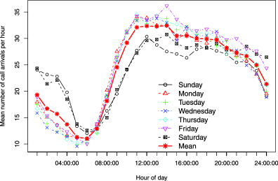
Figure 1: Mean number of calls per hour by day of the week.

As shown in Figure 1, the pattern of call arrivals over the course of a typical day has a distinct shape. After quickly increasing in the late morning, it peaks in the early afternoon, then slowly falls until it troughs between 5 and 6 a.m. See Section 4 for more discussion. In our analysis, we consider an arrival process that has been repeatedly observed over a particular time span, specifically, a 24 hour day. Let

$$\{y_{t}\dvtx t=1,\ldots,n\}\equiv\{y_{ij}\dvtx i=1,\ldots,d;j=1,\ldots,m\}$$

denote the sequence of call arrival counts, observed over time period $t$, which corresponds one-to-one with the $j$th sub-period of the $i$th day, so that $n=dm$. Our baseline approach is to model the arrival intensity $\lambda_{t}$ for the distinct shape of intraday call arrivals using a small number of smooth curves.

We consider two disjoint information sets for predictive conditioning. Let $\mathcal{F}_{t}=\sigma(Y_{1},\ldots,Y_{t})$ denote the $\sigma$-field generated by $Y_{1},\ldots,Y_{t}$, and let $\mathbf{X}=\{\mathbf{x}_{1},\ldots,\mathbf{x}_{n}\}$ denote any available deterministic covariate information about each observation. We incorporate calendar information such as day-of-week and week-of-year in our analysis. We define $\lambda_{t}$ as the conditional expectation of $Y_{t}$ given $\mathcal{F}_{t-1}$ and $\mathbf{X}$. We defined this above as the mean of $Y_{t}$. In our model these coincide; however, this mean may not be the same as the conditional expectation since $\lambda_{t}$ may depend on other unobserved random variables. Let $\mu_{t}=E(Y_{t}|\mathbf{X})>0$ denote the conditional mean of $Y_{t}$ given only the covariates $\mathbf{X}$. Let

$$\lambda_{t}=E(Y_{t}|\mathcal{F}_{t-1},\mathbf{X})=\mu_{t}E({Y_{t}}/{\mu_{t}}|\mathcal{F}_{t-1},\mathbf{X})=\mu_{t}\eta_{t},$$ (1)

in which $\eta_{t}>0$ is referred to as the conditional intensity inflation rate (CIIR). By construction,

$$E(\eta_{t}|\mathbf{X})=E(E({Y_{t}}|\mathcal{F}_{t-1},\mathbf{X})|\mathbf{X})/{\mu_{t}}=E({Y_{t}}|\mathbf{X})/{\mu_{t}}=1.$$

The CIIR process is intended to model any remaining serial dependence in call arrival counts after accounting for available covariates. In the EMS context we hypothesize that this dependence is due to sporadic events such as inclement weather or unusual traffic patterns. Since information regarding these events may not be available or predictable in general, we argue that an approach such as ours which explicitly models the remaining serial dependence will lead to improved short-term forecast accuracy. In Section 3 we consider a dynamic latent factor model estimated with smoothing splines for modeling $\mu_{t}$, various time series models for modeling $\eta_{t}$, and finally a conditional likelihood algorithm for estimating the latent intensity process $\lambda_{t}$ via estimation of $\eta_{t}$ given $\mu_{t}$.

The call arrival data used consists of all emergency priority calls received by Toronto EMS between January 1, 2007 and December 31, 2008 for which an ambulance was dispatched. This includes some calls not requiring lights-and-sirens response, but does not include scheduled patient transfers. We include only the first call arrival time in our analysis when multiple calls are received for the same event. The data were processed to exclude calls with no reported location. These removals totaled less than 1% of the data.

Many calls resulted in multiple ambulances being dispatched. Exploratory analysis revealed that the number of ambulances deployed for a single emergency did not depend on the day of the week, the week of the year, or exhibit any serial dependence. However, such instances were slightly more prevalent in the morning hours. Our analysis of hourly ambulance demand defines an event as a call arrival if one or more ambulances are deployed.

We removed seven days from the analysis because there were large gaps, over at least two consecutive hours, in which no emergency calls were received. These days most likely resulted from malfunctions in the computer-aided dispatch system which led to failures in recording calls for extended periods. Strictly speaking, it is not necessary to remove the entire days; however, we did so since it had a negligible impact on our results and it greatly simplified out-of-sample forecast comparisons and implementation of the simulation studies in Section 4.

Finally, we gave special consideration to holidays. We found that the intraday pattern on New Year’s Eve and Day was fundamentally different from the rest of the year and removed these days from our analysis. This finding is similar to the conclusions of Channouf et al. (2007) who found that New Year’s Day and the dates of the Calgary Stampede were the only days requiring special consideration in their methodology when applied to the city of Calgary. In practice, staffing decisions for holidays require special planning and consideration of many additional variables.

3 Modeling

Factor models provide a parsimonious representation of high dimensional data in many applied sciences, for example, econometrics [cf. Stock and Watson (2002)]. We combine a dynamic latent factor model with integer-valued time series models. We include covariates via simple constraints on the factor loadings. We estimate the model using smoothing splines to impose smooth evolution in the factor levels and loadings. The factor model provides a parsimonious representation of the nonstationary pattern in intraday call arrivals, while the time series models capture the remaining serial dependence in the arrival rate process.

3.1 Dynamic latent factor model

For notational simplicity, assume $m$ consecutive observations per day are available for $d$ consecutive days with no omissions in the record. Let $\mathbf{Y}=(y_{ij})$ denote the $d\times m$ matrix of observed counts for each day $i$ over each sub-period $j$. Let $\mu_{ij}=E(Y_{ij}|{\mathbf{X}})$, and let $\mathbf{M}=(\mu_{ij})$ denote the corresponding $d\times m$ latent nonstationary intensity matrix. To reduce the dimension of the intensity matrix $\mathbf{M}$, we introduce a $K$-factor model.

We assume that the intraday pattern of expected hourly call arrivals on the log scale can be well approximated by a linear combination of (a small number) $K$ factors or functions, denoted by $\mathbf{f}_{k}$ for $k=1,\ldots,K$. The factors are orthogonal length-$m$ vectors. The intraday arrival rate model $\bolds{\mu}_{i}$ over a particular day $i$ is given by

$$\log\bolds{\mu}_{i}={L_{i1}}{\mathbf{f}_{1}}+\cdots+{L_{iK}}{\mathbf{f}_{K}}.$$ (2)

Each of the factors $\mathbf{f}_{k}$ varies as a function over the periods within a day, but they are constant from one day to the next. Day-to-day changes are modeled by allowing the various factor loadings $L_{ik}$ to vary across days. When $K$ is much smaller than either $m$ or $d$, the dimensionality of the general problem is greatly reduced. In practice, $K$ must be chosen by the practitioner; we provide some discussion on choosing $K$ in Section 4.

In matrix form we have

$$\log\mathbf{M}=\mathbf{L}\mathbf{F}^{\mathrm{T}},$$ (3)

in which $\mathbf{F}=(\mathbf{f}_{1},\ldots,\mathbf{f}_{K})$ denotes the $m\times K$ matrix of underlying factors and $\mathbf{L}$ denotes the corresponding $d\times K$ matrix of factor loadings, both of which are assumed to have full column rank. Although other link functions are available, the component-wise log transformation implies a multiplicative structure among the $K$ common factors and ensures a positive estimate of each hourly intensity $\mu_{ij}$. Since neither $\mathbf{F}$ nor $\mathbf{L}$ are observable, the expression (3) is not identifiable. We further require $\mathbf{F}^{\mathrm{T}}\mathbf{F}=\mathbf{I}$ to alleviate this ambiguity and we iteratively estimate $\mathbf{F}$ and $\mathbf{L}$.

3.2 Factor modeling with covariates via constraints

To further reduce the dimensionality, we impose a set of constraints on the factor loading matrix $\mathbf{L}$. Let $\mathbf{H}$ denote a $d\times r$ full rank matrix ($r<d$) of given constraints (we discuss later what these should be for EMS). Let $\mathbf{B}$ denote an $r\times K$ matrix of unconstrained factor loadings. These unconstrained loadings $\mathbf{B}$ linearly combine to constitute the constrained factor loadings $\mathbf{L}$, such that $\mathbf{L}=\mathbf{H}\mathbf{B}$. Our factor model may now be written as

$$\log\mathbf{M}=\mathbf{L}\mathbf{F}^{\mathrm{T}}=\mathbf{H}\mathbf{B}\mathbf{F}^{\mathrm{T}}.$$

A considerable reduction in dimensionality occurs when $r$ is much smaller than $d$.

Constraints to assure identifiability are standard in factor analysis. The constraints we now consider incorporate auxiliary information about the rows and columns of the observation matrix $\mathbf{Y}$ to simplify estimation and to improve out-of-sample predictions. Similar constraints have been used in Takane and Hunter (2001), Tsai and Tsay (2010) and Matteson and Tsay (2011).

For example, the rows of $\mathbf{H}$ might consist of incidence vectors for particular days of the week, or special days which might require unique loadings on the common factors. We may choose to constrain all weekdays to have identical factor loadings and similarly constrain weekend days. However, this approach is much more general than simple equality constraints, as demonstrated below.

The intraday pattern of hourly call arrivals varies from one day to the next, although the same general shape is maintained. As seen in Figure 1, different days of the week exhibit distinct patterns. We do not observe large changes from one week to the next, but there are significant changes over the course of the year. We allow loadings to slowly vary from week to week. Both of these features are incorporated into the factor loadings $\mathbf{L}$ by specifying appropriate constraints $\mathbf{H}$. Let

$$\log\mathbf{M}=\mathbf{L}\mathbf{F}^{\mathrm{T}}=\mathbf{H}\mathbf{B}\mathbf{F}^{\mathrm{T}}=\pmatrix{\mathbf{H}^{(1)}&\mathbf{H}^{(2)}}\pmatrix{\mathbf{B}^{(1)}\cr\mathbf{B}^{(2)}}\mathbf{F}^{\mathrm{T}},$$ (4)

in which the first term corresponds to day-of-week effects and the second to smoothly varying week-of-year effects. $\mathbf{H}^{(1)}$ is a $d\times 7$ matrix in which each row $\mathbf{H}^{(1)}_{i}$ is an incidence vector for the day-of-week. Similarly, $\mathbf{H}^{(2)}$ is a $d\times 53$ matrix in which each row $\mathbf{H}^{(2)}_{i}$ is an incidence vector for the week-of-year. (We use a 53 week year since the first and last weeks may have fewer than 7 days.) The $7\times K$ matrix $\mathbf{B}^{(1)}=(\mathbf{b}^{(1)}_{1},\ldots,\mathbf{b}^{(1)}_{K})$ contains unconstrained factor loadings for the day-of-week and $\mathbf{B}^{(2)}=(\mathbf{b}^{(2)}_{1},\ldots,\mathbf{b}^{(2)}_{K})$ is a $53\times K$ matrix of factor loadings for the week-of-year.

3.3 Factor model estimation via smoothing splines

We assume that as the nonstationary intensity process $\mu_{ij}$ varies over the hours $j$ of each day $i$, it does so smoothly. If each of the common factors $\mathbf{f}_{k}\in\mathbb{R}^{m}$ varies smoothly over sub-periods $j$, then the smoothness of $\mu_{ij}$ is guaranteed for each day. Increasing the number of factors reduces possible discontinuities between the end of one day and the beginning of the next. To incorporate smoothness into the model (2), we use Generalized Additive Models (GAMs) in the estimation of the common factors $\mathbf{f}_{k}$. GAMs extend generalized linear models, allowing for more complicated relationships between the response and predictors by modeling some predictors nonparametrically [see, e.g., Hastie and Tibshirani (1990); Wood (2006)]. GAMs have been successfully used for count-valued data in the study of fish populations [cf. Borchers et al. (1997); Daskalov (1999)]. The factors $\mathbf{f}_{k}={f}_{k}(j)$ are a smooth function of the intraday time index covariate $j$. The loadings $\mathbf{L}$ are defined as before. If the loadings $\mathbf{L}$ were known covariates, equation (2) would be a varying coefficient model [cf. Hastie and Tibshirani (1993)].

There are several excellent libraries available in the statistical package R [R Development Core Team (2009)] for fitting GAMs, thus making them quite easy to implement. We used the gam function from the mgcv library [Wood (2008)] extensively. Other popular libraries include the gam package [Hastie (2009)] and the gss package [Gu (2010)]. See Wood [(2006), Section 5.6] for an introduction to GAM estimation using R.

In estimation of the model (2) via the gam function, we have used thin plate regression splines with a ten-dimensional basis, the Poisson family, and the log-link function. Thin plate regression splines are a low rank, isotropic smoother with many desirable properties. For example, no decisions on the placement of knots is needed. They are an optimal approximation to thin plate splines and, with the use of Lanczos iteration, they can be fit quickly even for large data sets [cf. Wood (2003)].

When the factors $\mathbf{F}$ are treated as a fixed covariate, the factor model can again be interpreted as a varying coefficient model. Given the calendar covariates $\mathbf{X}$, let

$$\log{\mu}_{ij} = {F}_{j1}L^{\mathrm{T}}_{1i}+\cdots+{F}_{jK}L^{\mathrm{T}}_{Ki}$$

$$= \sum_{k=1}^{K}{F}_{jk}\bigl{\{}{\mathbf{H}^{(1)\mathrm{T}}_{i}}\mathbf{b}_{k}^{(1)}+\mathbf{H}^{(2)\mathrm{T}}_{i}\mathbf{b}_{k}^{(2)}\bigr{\}}$$

$$= \sum_{k=1}^{K}{F}_{jk}\bigl{\{}{b}_{k}^{(1)}(\mathbf{x}_{i})+{b}_{k}^{(2)}(\mathbf{x}_{i})\bigr{\}},$$

in which ${b}_{k}^{(1)}(\mathbf{x}_{i})$ is a piece-wise constant function of the day-of-week, and ${b}_{k}^{(2)}(\mathbf{x}_{i})$ is a smoothly varying function over the week-of-year. We may again proceed with estimation via the gam function in R. Day-of-week covariates are simply added to the linear predictor as indicator variables. These represent a level shift in the daily loadings on each of the factors $\mathbf{f}_{k}$. In our application it is appropriate to assume a smooth transition between the last week of one year and the first week of the next. To ensure this in estimation of ${b}_{k}^{(2)}(\mathbf{x}_{i})$, we use a cyclic cubic regression spline for the basis [cf. Wood (2006), Section 5.1]. Iterative estimation of $\mathbf{F}$, and $\mathbf{L}$ via $\mathbf{B}$, for a given number of factors $K$ is discussed in Section 3.5.

We allow the degree of smoothness for the factors ${f}_{k}$ and the loadings function ${b}_{k}^{(2)}(\mathbf{x}_{i})$ to be automatically estimated by generalized cross validation (GVC). We expect short term serial dependence in the residuals for our application. For smoothing methods in general, if autocorrelation between the residuals is ignored, automatic smoothing parameter selection may break down [see, e.g., Opsomer, Wang and Yang (2001)]. The proposed factor model may be susceptible to this if the number of days included is not sufficiently large compared to the number of smooth factors and loadings, or if the residuals are long-range dependent. We use what is referred to as a performance iteration [cf. Gu (1992)] versus an outer iteration strategy which requires repeated estimation for many trial sets of the smoothing parameters. The performance iteration strategy is much more computationally efficient for use in the proposed algorithm, but convergence is not guaranteed, in general. In particular, cycling between pairs of smoothing parameters and coefficient estimates may occur [cf. Wood (2006), Section 4.5], especially when the number of factors $K$ is large.

3.4 Adaptive forecasting with time series models

Let $\widehat{e}_{t}=Y_{t}/\widehat{\mu}_{t}$ denote the multiplicative residual in period $t$ implied by the fitted values $\widehat{\mu}_{t}$ from a factor model estimated as described in the previous sections. Time series plots of this residual process appear stationary, but exhibit some serial dependence. In this section we consider time series models for the latent CIIR process $\eta_{t}=E({Y_{t}}/{\mu_{t}}|\mathcal{F}_{t-1},\mathbf{X})$ to account for this dependence.

To investigate the nature of the serial dependence, we study the bivariate relationship between the $\widehat{e}_{t}$ process versus several lagged values of the process $\widehat{e}_{t-\ell}$. Scatterplots reveal a roughly linear relationship. Residual autocorrelation and partial autocorrelation plots for one of the factor models fit in Section 4 are given in Figure 5(b) and (c). These quantify the strength of the linear relationship as the lag $\ell$ increases. It appears to persist for many periods, with an approximately geometric rate of decay as the lag increases.

To explain this serial dependence, we first consider a generalized autoregressive linear model, defined by the recursion

$$\eta_{t}=\omega+\alpha\widehat{e}_{t-1}+\beta\eta_{t-1}.$$ (6)

To ensure positivity, we restrict $\omega>0$ and $\alpha,\beta\geq 0$. When $\mu_{t}$ is constant, the resulting model for $Y_{t}$ is an $\operatorname{Integer\mbox{-}GARCH}(1,1)$ (IntGARCH) model [e.g., Ferland, Latour and Oraichi (2006)]. It is worth noting some properties of this model for the constant $\mu_{t}$ case. To ensure the stationarity of $\eta_{t}$, we further require that $\alpha+\beta<1$. This sum determines the persistence of the process, with larger values of $\alpha$ leading to more adaptability. When this stationarity condition is satisfied, and $\eta_{t}$ has reached its stationary distribution, the expectation of $\eta_{t}$ given ${\mathbf{X}}$ is

$$E(\eta_{t}|{\mathbf{X}})=\omega/(1-\alpha-\beta).$$

To ensure $E(\eta_{t}|{\mathbf{X}})=1$ for the fitted model, we may parameterize $\omega=1-\alpha-\beta$. This constraint is simple enough to enforce for the model (6) and we do so. However, additional parameter constraints such as this may make numerical estimation intractable in more complicated models and they are not enforced by us in the models outlined below.

When $\mu_{t}$ is a nonstationary process, the conditional intensity

$$\lambda_{t}=\mu_{t}\eta_{t}$$

is also nonstationary. Since $E(\eta_{t}|{\mathbf{X}})=1$, we interpret $\eta_{t}$ as the stationary multiplicative deviation, or inflation rate, between $\lambda_{t}$ and $\mu_{t}$. The $\lambda_{t}$ process is mean reverting to the $\mu_{t}$ process. Let

$$\widehat{\varepsilon}_{t}=Y_{t}/\widehat{\lambda}_{t}$$

denote the multiplicative standardized residual process given an estimated CIIR process $\widehat{\eta}_{t}$. If a fitted model defined by (6) sufficiently explains the observed linear dependence in $\widehat{e}_{t}$, then an autocorrelation plot of $\widehat{\varepsilon}_{t}$ should be statistically insignificant for all lags $\ell$. As a preview, the standardized residual autocorrelation plot for one such model fit in Section 4 is given in Figure 5(d). The serial correlation appears to have been adequately removed.

Next, we formulate three different nonlinear generalizations of (6) that may better characterize the serial dependence, and possibly lead to improved forecasts. The first is an exponential autoregressive model defined as

$$\eta_{t} = \alpha\widehat{e}_{t-1}+[\beta+\delta\exp(-\gamma\eta_{t-1}^{2})]\eta_{t-1},$$ (7)

in which $\alpha,\beta,\delta,\gamma>0$. Exponential autoregressive models are attractive in application because of their threshold-like behavior. For large $\eta_{t-1}$, the functional coefficient for $\eta_{t-1}$ is approximately $\beta$, and for small $\eta_{t-1}$ it is approximately $\beta+\delta$. Additionally, the transition between these regimes remains smooth. As in Fokianos, Rahbek and Tjøstheim (2009), for $\alpha+\beta<1$ one can verify the $\eta_{t}$ process has a stationarity version when $\mu_{t}$ is constant.

We also consider a piecewise linear threshold model

$$\eta_{t}=\omega+\alpha\widehat{e}_{t-1}+\beta\eta_{t-1}+(\gamma\widehat{e}_{t-1}+\delta\eta_{t-1})I_{\{\widehat{e}_{t-1}\notin(c_{1},c_{2})\}},$$ (8)

in which $I$ is an indicator variable and the threshold boundaries satisfy $0<c_{1}<1<c_{2}<\infty$. To ensure positivity of $\eta_{t}$, we assume $\omega,\alpha,\beta>0$, $(\alpha+\gamma)>0$, and $(\beta+\delta)>0$. Additionally, we take $\delta\leq 0$ and $\gamma\geq 0$, such that when $\widehat{e}_{t-1}$ is outside the range $(c_{1},c_{2})$ the CIIR process $\eta_{t}$ is more adaptive, that is, puts more weight on $\widehat{e}_{t-1}$ and less on $\eta_{t-1}$. When $\mu_{t}$ is constant, the $\eta_{t}$ process has a stationary version under the restriction $\alpha+\beta+\gamma+\delta<1$; see Woodard, Matteson and Henderson (2010). In practice, the threshold boundaries $c_{1}$ and $c_{2}$ are fixed during estimation, and may be adjusted as necessary after further exploratory analysis. We chose $c_{1}=1/1.15$ and $c_{2}=1.15$, that is, thresholds at 15% above and below 1.

Finally, we consider a model with regime switching at deterministic times, letting

$$\qquad\eta_{t}=(\omega_{1}+\alpha_{1}\widehat{e}_{t-1}+\beta_{1}\eta_{t-1})I_{\{t\in(t_{1},t_{2})\}}+(\omega_{2}+\alpha_{2}\widehat{e}_{t-1}+\beta_{2}\eta_{t-1})I_{\{t\notin(t_{1},t_{2})\}}.$$ (9)

This model is appropriate assuming the residual process has two distinct regimes for different periods of the day. For example, one regime could be for normal workday hours with the other regime being for the evening and early morning hours. No stationarity is possible for this model. A drawback of this model is that the process has jumps at $t_{1}$ and $t_{2}$. As was the case for $c_{1}$ and $c_{2}$ in (8), $t_{1}$ and $t_{2}$ are fixed during estimation. After exploratory analysis, we chose $t_{1}=10$ a.m. and $t_{2}=4$ p.m.

3.5 Estimation algorithm

The estimation procedure below begins with an iterative algorithm for estimating the factor model from Sections 3.1–3.3 through repeated use of the gam function from the mgcv library in R. Any serial dependence is ignored during estimation of $\mu_{t}$ for simplicity. Given estimates for the factor model $\widehat{\mu}_{t}$, conditional maximum likelihood is used to estimate the conditional intensity $\lambda_{t}$ via one of the time series models given in (6)–(9) for the CIIR process $\eta_{t}$.

1. Initialization:

   1. [(a)]

   2. Fix $K$ and $\mathbf{H}$.

   3. Choose some $c\in(0,1)$ and define $\mathbf{Y}_{c}=(y_{ij}\vee c)$.

   4. Apply a singular value decomposition (SVD) to find $\log(\mathbf{Y}_{c})=\break\mathbf{U}_{0}\mathbf{D}_{0}\mathbf{V}^{\mathrm{T}}_{0}$.

      1. [(iii)]

      2. Let $\mathbf{U}_{0}^{(1:K)}$ denote the first $K$ columns of the left singular matrix $\mathbf{U}_{0}$.

      3. Let $\mathbf{V}_{0}^{(1:K)}$ denote the first $K$ columns of the right singular matrix $\mathbf{V}_{0}$.

      4. Let $\mathbf{D}_{0}^{(1:K)}$ denote the upper-left $K\times K$ sub-matrix of $\mathbf{D}_{0}$, the diagonal matrix of singular values.

   5. Assign $\mathbf{L}_{0}=\mathbf{U}_{0}^{(1:K)}\mathbf{D}_{0}^{(1:K)}$ and $\mathbf{F}_{0}=\mathbf{V}_{0}^{(1:K)}$.

   6. No smoothing is performed and the constraints $\mathbf{H}$ are omitted in initialization.

2. Update:

   1. [(a)]

   2. Fit the Poisson GAM model described in Section 3.3 with $\mathbf{F}=\mathbf{F}_{n}$ and $\mathbf{H}$ as fixed covariates.

      • Assign $\mathbf{B}_{n^{*}}$ as the estimated parameter values from this fit and let $\mathbf{L}_{n^{*}}=\mathbf{H}\mathbf{B}_{n^{*}}$.

   3. Fit the Poisson GAM model described in Section 3.3 with $\mathbf{L}=\mathbf{L}_{n^{*}}$ as a fixed covariate.

      • Assign $\mathbf{F}_{n^{*}}$ as the estimated parameter values from this fit.

   4. Apply an SVD to find $\mathbf{B}_{n^{*}}\mathbf{F}_{n^{*}}^{\mathrm{T}}=\mathbf{U}_{n+1}\mathbf{D}_{n+1}\mathbf{V}^{\mathrm{T}}_{n+1}$.

      1. [(iii)]

      2. Assign $\mathbf{B}_{n+1}=\mathbf{U}_{n+1}^{(1:K)}\mathbf{D}_{n+1}^{(1:K)}$.

      3. Assign $\mathbf{F}_{n+1}=\mathbf{V}_{n+1}^{(1:K)}$.

      4. Assign $\mathbf{L}_{n+1}=\mathbf{H}\mathbf{B}_{n+1}$.

   5. Let $\log\mathbf{M}_{n+1}=\mathbf{L}_{n+1}\mathbf{F}_{n+1}^{\mathrm{T}}$.

3. Repeat the update steps recursively until convergence.

Convergence is reached when the relative change in $\mathbf{M}$ is sufficiently small. After convergence we can recover $\log\widehat{\mu_{t}}$ from the rows of the final estimate of $\log\mathbf{M}$. These values are then treated as fixed constants during estimation of $\eta_{t}$. We use conditional maximum likelihood to estimate the parameters $(\omega,\alpha,\beta,\ldots)$ associated with a time series model for $\eta_{t}$. The recursion defined by (6)–(9) requires initialization by choosing a value for $\eta_{1}$; the estimates are conditional on the chosen initialization.

We may always specify the joint distribution $P_{\mathbf{Y}}$ of the observations $\mathbf{Y}$ as an iterated product of successive conditional distributions $P_{Y_{t}}$ for $Y_{t}$ given $(Y_{t-1},\ldots,Y_{1})$ as

$$P_{Y}(y_{T},y_{T-1},\ldots,y_{2},y_{1})=P_{Y_{1}}(y_{1})\prod_{t=2}^{T}P_{Y_{t}}(y_{t}|y_{t-1},\ldots,y_{1}).$$

We follow the standard convention of fixing $P_{Y_{1}}(y_{1})=1$ in estimation. For large sample sizes the practical impact of this decision is negligible. We may therefore write the log likelihood function as the sum of iterated conditional log likelihood functions. The conditional distribution for the observations is assumed to be Poisson with mean $\lambda_{t}={\mu}_{t}\eta_{t}.$

For uninterrupted observations over periods $1,\ldots,T,$ we define the log likelihood function as

$${\ell}(\omega,\alpha,\beta,\ldots|\widehat{M},Y,\eta_{1}) = \sum_{t=2}^{T}\ell_{t}(\omega,\alpha,\beta,\ldots|y_{t},y_{t-1},\widehat{\mu}_{t},\widehat{\mu}_{t-1},\eta_{t-1})$$

$$= \sum_{t=2}^{T}(y_{t}\log\lambda_{t}-\lambda_{t}-\log y_{t}!)$$

$$= \sum_{t=2}^{T}\bigl{(}y_{t}\log(\widehat{\mu}_{t}\eta_{t})-\widehat{\mu}_{t}\eta_{t}-\log y_{t}!\bigr{)}.$$

This recursion requires an initial value for $\eta_{1}$. For simplicity, we use its expected value, $\eta_{1}=1$. When there are gaps in the observation record, equation (3.5) is calculated over every contiguous block of observations. This requires reinitialization of $\eta_{t}=1$ at the beginning of each block. The log likelihood for the blocks are then added together to form the entire log likelihood. The maximum likelihood estimate is the $\mathrm{argmax}$ of this quantity, subject to the constraints given in Section 3.4. Finally, $\eta_{t}$ is estimated by the respective recursion given by equations (6)–(9) with parameters replaced by their estimates, again with reinitialization of $\eta_{t}=1$ at the beginning of each contiguous block of observations. Blocks were large enough in our application that the effect of reinitialization was negligible.

4 Empirical analysis

Using the data described in Section 2, we perform the following analysis: (a) we define various statistical goodness-of-fit metrics suitable for the proposed models; based on in-sample performance, these metrics are used to determine the number of factors $K$ for use in the dynamic factor models. (b) We compare the out-of-sample forecast performance for the factor model in (3), the factor model with constraints in (4), and the factor model with constraints and smoothing splines in (3.3). These comparisons help ascertain the improvement from each refinement and validate the proposed selection methods for $K$. (c) For the latter factor model, we compare the out-of-sample forecast performance with the addition of the CIIR process, via use of the various time series models defined in Section 3.4. (d) We quantify the practical impact of these successive statistical improvements with a queueing application constructed to approximate ambulance operations.

4.1 Interpreting the fitted model

The mean number of calls was approximately 24 per hour for 2007 and 2008, and no increasing or decreasing linear trend in time was detected during this period. We partition the observations by year into two data sets referred to as 2007 and 2008, respectively. Each year is first regarded as a training set, and each model is fit individually to each year. The opposite year is subsequently used as a test set to evaluate the out-of-sample performance of each fitted model. To account for missing days, we reinitialize the CIIR process $\eta_{t}$ in the first period following each day of missing data. This was necessary at most five times per year including the first day of the year.

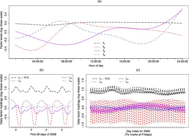
Figure 2: 2008 fitted (a) factor levels $\mathbf{f}_{k}$ (log-linear scale) and [(b) and (c)] corresponding factor loadings $\mathbf{L}_{k\cdot}$ (log-linear scale) for a factor model fit with constraints, smoothing splines and $K=4$ factors. $(\mathbf{L}_{1\cdot}-14.5)$ is shown for easier comparison.

We found the factor model fit with constraints, smoothing splines, and $K=4$ factors to be the most appropriate of the factor models considered. The estimated factors $\mathbf{f}_{k}$ for 2008 are shown in Figure 2(a). Each of the four factors varies smoothly over the hours of the day via use of smoothing splines. The first factor $\mathbf{f}_{1}$ is strictly positive and the least variable. It appears to capture the mean diurnal pattern. The factor $\mathbf{f}_{2}$ appears to isolate the dominant relative differences between weekdays and weekend days. The defining feature of $\mathbf{f}_{3}$ and $\mathbf{f}_{4}$ is the large increase late in the day, corresponding closely to the relative increase observed on Friday and Saturday evenings. However, $\mathbf{f}_{3}$ decreases in the morning, while $\mathbf{f}_{4}$ increases in the morning and decreases in the late afternoon. As $K$ increases, additional factors become increasingly more variable over the hours of the day. Too many factors result in overfitting the model, as the extra factors capture noise.

The corresponding daily factor loadings $\mathbf{L}$ for the first four weeks of 2008 are shown in Figure 2(b). The loadings $(\mathbf{L}_{1}-14.5)$ are shown to simplify comparisons. The much higher loadings on $\mathbf{f}_{1}$ confirm its interpretation as capturing the mean. The peaks on Fridays coincide with Friday having the highest average number of calls, as seen in Figure 1. Weekdays get a positive loading on $\mathbf{f}_{2}$, while weekend days get negative loading. Loadings on $\mathbf{f}_{3}$ are lowest on Sundays and Mondays and loadings on $\mathbf{f}_{4}$ are largest on Fridays and Saturdays. As $K$ increases, the loadings on additional factors become increasingly close to zero. This partially mitigates the overfitting described above. Factors with loadings close to zero have less impact on the fitted values $\widehat{\mu}_{t}$. Nevertheless, they can still reduce out-of-sample forecast performance.

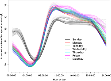
Figure 3: The estimated intensity process $\hat{\bolds{\mu}}_{i}$, for every day in 2008, for a factor model fit with constraints, smoothing splines and $K=4$ factors, colored by day-of-week, and shaded light to dark by week-of-year.

The daily factor loadings for all of 2008 are shown in Figure 2(c). The relative magnitude of each loading vector with respect to day-of-week is constant. This results from use of the constraint matrix $\mathbf{H}^{(1)}$ in (4). As the loadings vary over the days of the week, they also vary smoothly over the course of the year, via use of the constraint matrix $\mathbf{H}^{(2)}$ and the use of cyclic smoothing splines in estimation of $\mathbf{B}^{(2)}$ in (4). The loadings on $\mathbf{f}_{1}$ show how the expected number of calls per day varies over the year. The week to week variability in the other loadings influences how the days of the week change relative to each other over the year. Figure 3 shows the estimated intensity process $\widehat{\bolds{\mu}}_{i}$ for every day in 2008, shaded by day-of-week. The curves vary smoothly over the hours of the day. The fit for each day of the week keeps the same relative shape, but it varies smoothly over the weeks of the year.

Section 3.4 described incorporating time series models to improve the short-term forecasts of a factor model. The models capture the observed serial dependence in the multiplicative residuals from a fitted factor model; see Figure 5. Parameter estimates and approximate standard errors for the IntGARCH model are given in Supplemental material (Table 1). A fitted factor model $\widehat{\mu}_{t}$ using constraints, smoothing splines and $K=4$, as well as the factor model including a fitted $\operatorname{IntGARCH}(1,1)$ model $\widehat{\lambda}_{t}$, are also shown in Figure 6(a), with the observed call arrivals per hour for Weeks 8 and 9 of 2007. The $\widehat{\lambda}_{t}$ process is mean reverting about the $\widehat{\mu}_{t}$ process. They are typically close to each other, but when they differ by a larger amount, they tend to differ for several hours at a time. The corresponding fitted CIIR process $\widehat{\eta}_{t}$ is shown in Figure 6(b). This clearly illustrates the dependence and persistence exhibited in Figure 6(a). The CIIR process ranges between $\pm$6% during this period. With a mean of 24 calls per hour, this range corresponds to $\widehat{\lambda}_{t}$ varying about $\widehat{\mu}_{t}$ by about $\pm$1.5 expected calls per hour.

4.2 Goodness of fit and model selection

To evaluate the fitted values and forecasts of the proposed models, three types of residuals are computed: multiplicative, Pearson and Anscombe. Their respective formulas for the Poisson distribution are given by

$$\widehat{r}_{M,t}=\frac{y_{t}}{{\widehat{\lambda}_{t}}}-1,\qquad\widehat{r}_{P,t}=\frac{y_{t}-\widehat{\lambda}_{t}}{\sqrt{\widehat{\lambda}_{t}}},\qquad\widehat{r}_{A,t}=\frac{({3}/{2})(y_{t}^{2/3}-\widehat{\lambda}_{t}^{2/3})}{\widehat{\lambda}_{t}^{1/6}}.$$

We refer to the root mean square error (RMSE) of each metric as RMSME, RMSPE and RMSAE, respectively. The multiplicative residual is defined as before and is a natural choice given the definition for the CIIR. Since the variance of a Poisson random variable is equal to its mean, the Pearson residual is quite standard. However, the Pearson residual can be quite skewed for the Poisson distribution [cf. McCullagh and Nelder (1989), Section 2.4]. The Anscombe residual is derived as a transformation that makes the distribution of the residuals as close to Gaussian as possible while suitably scaling to stabilize the variance. See Pierce and Schafer (1986) for further discussion of residuals for generalized linear models. While the three methods always yielded the same conclusion, we found use of the Anscombe residuals gave a more robust assessment of model accuracy and simplified paired comparisons between the residuals of competing models.

The three RMSE metrics were used for both in- and out-of-sample model comparisons. For in-sample comparisons of the factor models, we also computed the deviance of each fitted model $\widehat{\mu}_{t}$. As a goodness-of-fit metric, deviance is derived from the logarithm of a ratio of likelihoods. For a log likelihood function $\ell(\bolds{\mu}|\mathbf{Y})$, it is defined as

$$-2\{\ell(\bolds{\mu}=\widehat{\bolds{\mu}}|\mathbf{Y})-\ell(\bolds{\mu}=\mathbf{Y}|\mathbf{Y})\},$$

in general. For a fitted factor model, ignoring serial dependence, the deviance corresponding to a Poisson distribution is

$$2\sum^{n}_{t=1}\{y_{t}\log(y_{t}/\widehat{\mu}_{t})-(y_{t}-\widehat{\mu}_{t})\},$$

in which the first term is zero if $y_{t}=0$.

We compare the fitted models’ relative reduction in deviance and RMSE as we increase the number of factors $K$. Figure 4 shows these results for factor models fit to 2007 data with constraints and smoothing splines. The results for other models and for 2008 were very similar. This plot may be interpreted similarly to a scree plot in PCA by identifying the point at which performance tapers off and the marginal improvement from additional factors is negligible. Under each scenario we consistently selected $K=4$ factors through this graphical criterion. To further justify this as a factor selection strategy, we also consider the impact the number of factors $K$ has on out-of-sample performance for each of the proposed models below. This approach is straightforward, but it does not fully account for the uncertainty on the number of factors. Bayesian estimation would require specialized computation, but it may improve model assessment [see, e.g., Lopes and West (2004)].

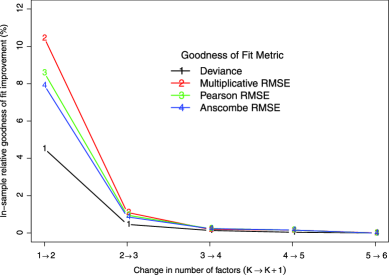
Figure 4: 2007 percentage in-sample relative goodness-of-fit improvement by addition of one factor ($K\rightarrow K+1$) for a factor model fit with constraints and smoothing splines.

Figure 5: (a) Sample autocorrelation function for hourly call arrival counts $y_{t}$. Residual $\widehat{e}_{t}=y_{t}/\widehat{\mu}_{t}$ (b) autocorrelation and (c) partial autocorrelation functions for fitted factor model $\widehat{\mu}_{t}$ with $k=4$ factors using factor and loading constraints and smoothing splines. (d) Standardized residual $\widehat{\varepsilon}_{t}=y_{t}/\widehat{\lambda}_{t}=y_{t}/(\widehat{\mu}_{t}\widehat{\eta}_{t})$ autocorrelation function for fitted factor model with fitted $\operatorname{IntGARCH}(1,1)$ model for $\eta_{t}$. Dashed lines give approximate 95% confidence levels.

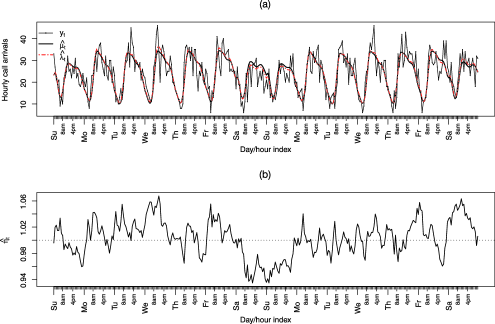
Figure 6: Weeks 8 and 9 of 2007: (a) observed call arrivals per hour $y_{t}$, fitted $K=4$ dynamic factor model $\widehat{\mu}_{t}$ using constraints and smoothing splines, and factor model $\widehat{\lambda}_{t}$ including fitted $\operatorname{IntGARCH}(1,1)$; (b) the fitted conditional intensity inflation process $\widehat{\eta}_{t}$ from the $\operatorname{IntGARCH}(1,1)$ model.

4.3 Out-of-sample forecast performance

Out-of-sample comparisons were made by fitting models to the 2007 training set and forecasting on the 2008 test set, and vice versa. To make predictions comparable from one year to the next, we align corresponding calendar weeks of the year, not days of the year. This ensures that estimates for Sundays are appropriately compared to Sundays, etc.

The first model considered was the simple prediction (SP) method. This simple moving average involving four observations was defined in theIntroduction. Next, the forecasts of various factor models (FM) were considered. For $K=1,\ldots,6,$ we evaluated the forecasts from the FM in (3), the FM with constraints in (4), and the FM with constraints and smoothing splines in (3.3). Finally, for the latter FM, with $K=4$, we calculate the implied fit from the training set with the inclusion of the CIIR process via the various time series models defined in Section 3.4. We compute the forecast RMSE of each model for the three residual types, for both years.

== 2007 model, 2008 residuals 2008 model, 2007 residuals Model Constraint Smoothing RMSME RMSPE RMSAE RMSME RMSPE RMSAE Simple prediction NA NA 0.2696 1.1955 1.1849 0.2661 1.1902 1.1925 Factor model, $K=1$ No No 0.2722 1.2369 1.2237 0.2657 1.2183 1.2263 Factor model, $K=2$ No No 0.2721 1.2357 1.2225 0.2661 1.2197 1.2277 Factor model, $K=3$ No No 0.2727 1.2374 1.2239 0.2659 1.2182 1.2262 Factor model, $K=4$ No No 0.2729 1.2383 1.2249 0.2666 1.2206 1.2283 Factor model, $K=5$ No No 0.2732 1.2395 1.2260 0.2670 1.2220 1.2294 Factor model, $K=6$ No No 0.2733 1.2401 1.2270 0.2668 1.2217 1.2294 Factor model, $K=1$ Yes No 0.2638 1.1863 1.1756 0.2575 1.1633 1.1721 Factor model, $K=2$ Yes No 0.2402 1.0938 1.0888 0.2333 1.0722 1.0875 Factor model, $K=3$ Yes No 0.2392 1.0877 1.0829 0.2324 1.0688 1.0848 Factor model, $K=4$ Yes No 0.2413 1.0945 1.0889 0.2347 1.0761 1.0912 Factor model, $K=5$ Yes No 0.2425 1.0994 1.0933 0.2363 1.0817 1.0961 Factor model, $K=6$ Yes No 0.2436 1.1051 1.0988 0.2377 1.0858 1.0999 Factor model, $K=1$ Yes Yes 0.2633 1.1837 1.1731 0.2573 1.1615 1.1703 Factor model, $K=2$ Yes Yes 0.2371 1.0844 1.0805 0.2310 1.0643 1.0803 Factor model, $K=3$ Yes Yes 0.2347 1.0744 1.0710 0.2289 1.0561 1.0728 Factor model, $K=4$ Yes Yes 0.2344 1.0730 1.0696 0.2288 1.0549 1.0715 Factor model, $K=5$ Yes Yes 0.2347 1.0740 1.0706 0.2289 1.0549 1.0714 Factor model, $K=6$ Yes Yes 0.2347 1.0739 1.0705 0.2289 1.0551 1.0716 Time series and FM, $K=4$ Yes Yes – – – – – – IntGARCH – – 0.2308 1.0571 1.0570 0.2274 1.0442 1.0580 IntExpGARCH – – 0.2308 1.0570 1.0569 0.2274 1.0441 1.0579 IntThreshGARCH – – 0.2308 1.0571 1.0570 0.2275 1.0443 1.0580 IntRsGARCH – – 0.2299 1.0540 1.0554 0.2274 1.0433 1.0565 []A Yes in the constraints column implies that the factor model was fit using the constraints outlined in Section 3.2. A Yes in the smoothing column indicates that the model was fit using smoothing splines as described in Section 3.3.

Table 1: Root mean square multiplicative, Pearson, and Anscombe errors for fitting model to 2007 and forecasting 2008, and vice versa

The forecast results are shown in Table 1. The basic FMs did slightly worse than the SP both years. With only one year of observations, these FMs tend to overfit the training set data, even with a small number of factors. The FMs with constraints give a very significant improvement over the previous models. The forecast RMSE is lowest at $K=4$ for the 2007 test set, and at $K=3$ for the 2008 test set. There was also a very large decrease between $K=1$ and $K=2$. The FMs with constraints and smoothing splines offered an additional improvement. The forecast RMSE is lowest at $K=4$ for both test sets. With the addition of the IntGARCH model for the CIIR process to this model, the RMSE improved again. Application of the nonlinear time series models instead offered only a slight improvement over the IntGARCH model.

With only one year of training data, each FM begins to overfit with $K=5$ factors. Results were largely consistent regardless of the residual used, but the Anscombe residuals were the least skewed and allowed the simplest pairwise comparisons. Although the FMs with constraints had superior in-sample performance, the use of smoothing splines reduced the tendency to over-fit and resulted in improved forecast performance. The CIIR process offered improvements in fit over FMs alone.

We also fit each of the nonlinear time series models discussed in Section 3.4 using a FM with $K=4$. The regime switching model had the best performance. It had the lowest RMSE for both test sets. The exponential autoregressive and the piecewise linear threshold models performed similarly to the IntGARCH model for both test sets. Although the nonlinear models consistently performed better in-sample, their out-of-sample performance was similar to the IntGARCH model.

4.4 Queueing model simulation to approximate ambulance operations

To comprehensively improve ambulance operations, it would be advantageous to simultaneously model the service duration of dispatched ambulances in addition to the demand for ambulance service. Unfortunately, such information was not available. We are currently working with Toronto EMS to use our improved estimates of call arrival rates to improve staffing in their dispatch call center. Extending our approach to a spatial-temporal forecasting model will likely be used to help determine when and where to deploy ambulances.

We present a simulation study that uses a simple queueing system to quantify the impact that improved forecasts have on staffing decisions and relative operating costs, for the Toronto data. The queueing model is a simplification of ambulance operations that ignores the spatial component. Similar queueing models have been used frequently in EMS modeling [see Swersey (1994), page 173]. This goodness-of-fit measure facilitates model comparisons and a similar approach may be useful in other contexts.

We use the terminology employed in the call center and queueing theory literature throughout the section; for our application, servers are a proxy for ambulances, callers or customers are those requiring EMS, and a server completing service is equated to an ambulance completing transport of a person to a hospital, etc. As before, let $y_{t}$ denote the observed number of call arrivals during hour $t$. Our experiment examines the behavior of a simple $M/M/s$ queueing system. The arrival rate in time period $t$ is $\lambda_{t}$. During this period, let $s_{t}$ denote the number of servers at hand. For simplicity, we assume that the service rate $\nu$ for each server is the same, and constant over time. Furthermore, intra-hour arrivals occur according to a Poisson process with rate $\lambda_{t}$, and service times of callers are independent and exponentially distributed with rate $\nu$.

As in Section 4.3, models are calibrated on one year of observations and forecasts for $\lambda_{t}$ are made for the other year. Each model’s forecasts $\widehat{\lambda}_{t}$ are then used to determine corresponding staffing levels $\widehat{s}_{t}$ for the system.

To facilitate comparisons of short-term forecasts, we assume that the number of servers can be changed instantaneously at the beginning of each period. In practice, it is possible to adjust the number of ambulances in real time, but not to the degree that we assume here.

Each call has an associated arrival time and service time. When a call arrives, the caller goes immediately into service if a server is available, otherwise it is added to the end of the queue. A common goal in EMS is to ensure that a certain proportion of calls are reached by an ambulance within a prespecified amount of time. We approximate this goal by instead aiming to answer a proportion, $\theta$, of calls immediately; this is a standard approximation in queueing applications in many areas including EMS [Kolesar and Green (1998)]. For each call arrival, we note whether or not the caller was served immediately. As servers complete service, they immediately begin serving the first caller waiting in the queue, otherwise they await new arrivals if the queue is currently empty. One simulation replication of the queueing system simulates all calls in the test year.

To implement the queueing system simulation, it is first necessary to simulate arrival and service times for each caller in the forecast period. We use the observed number of calls for each hour $y_{t}$ as the number of arrivals to the system in period $t$. Since arrivals to the system are assumed to follow a Poisson process, we determine the $y_{t}$ call arrival times using the well-known result that, conditional on the total number of arrivals in the period $[t,t+1]$, the arrival times have the same distribution as the order statistics of $y_{t}$ independent Uniform($t,t+1$) random variables. We exploit this relationship to generate the intra-hour arrival times given the observed arrival volume $y_{t}$. The service times for each call are generated independently with an Exponential($\nu$) distribution.

The final input is the initial state of the queue within the system. We generate an initial number of callers in the queue as Poisson($y_{1}$), then independently generate corresponding Exponential($\nu$) residual service times for each of these callers. This initialization is motivated through an infinite-server model; see, for example, Kolesar and Green (1998). Whenever there is a missing day, in either the test set or corresponding training set period, we similarly reinitialize the state of the queue but with $y_{1}$ replaced by the number of calls observed in the first period following the missing period. These initializations are common across the different forecasting methods to allow direct comparisons.

To evaluate forecast performance, we define a cost function and an appropriate method for determining server levels from arrival rate estimates. Let $n_{t}$ denote the number of callers served immediately in period $t$. The hourly cost function is given by

$$C(n_{t},y_{t},s_{t})=\mathrm{Pen}(n_{t},y_{t})+s_{t},$$

in which

$$\mathrm{Pen}(n_{t},y_{t})=\cases{0,&\quad if $n_{t}\geq\theta y_{t}$,\cr q(y_{t}-n_{t}),&\quad otherwise,}$$

$\theta\in(0,1)$ is the targeted proportion of calls served immediately, and $q\geq 0$ is the cost of not immediately serving a customer, relative to the cost of staffing one server for one hour. The total cost, with respect to the hourly server cost, for the entire forecast period is

$$C=\sum_{t}C(n_{t},y_{t},s_{t})=\sum_{t}\mathrm{Pen}(n_{t},y_{t})+\sum_{t}s_{t}.$$

This approach, where penalties for poor service are balanced against staffing costs, is frequently used; see, e.g., Andrews and Parsons (1993), Harrison, Zeevi and Shum (2005).

At time $t-1$, the number of call arrivals and the number served immediately are random variables, denoted as $Y_{t}$ and $N_{t}$, respectively. A natural objective is to choose staffing levels that minimize the hourly expected cost as

$$\widehat{s}_{t}=\operatorname{argmin}\limits_{s_{t}\in\mathbb{N}}E\{C(N_{t},Y_{t},s_{t})|\mathcal{F}_{t-1},\mathbf{X}\},$$ (11)

in which $Y_{t}$ is assumed to have a Poisson distribution with mean equal to the arrival rate forecast $\widehat{\lambda}_{t}$. The staffing levels are then a function of arrival rate forecasts, $\widehat{s}_{t}(\widehat{\lambda}_{t})$. We approximate this expectation numerically by randomly generating $J$ independent realizations as $Y_{t,j}\sim\operatorname{Poisson}(\widehat{\lambda}_{t})$. Then, for each $Y_{t,j}$ we simulate one independent realization of $N_{t}$. For a fixed value of $s_{t}$ the expectation is approximated by ${J}^{-1}\sum_{t=1}^{J}\{\operatorname{Pen}(N_{t,j},Y_{t,j})+s_{t}\}$. We found that $J=25\mbox{,}000$ provided adequate accuracy.

Independent realizations of $N_{t}|Y_{t}$ require running the queueing system forward one hour, but this is very computationally intensive. To approximate $N_{t}|Y_{t}$, we use a Binomial distribution. Let $N_{t,j}|Y_{t,j}\sim\operatorname{Binomial}\{Y_{t,j},\break g(\widehat{\lambda}_{t},s_{t},\nu)\}$. The function $g$ gives the steady state probability that a customer is served immediately for a queueing system with a constant arrival rate, server level and service rate, $\widehat{\lambda}_{t},s_{t}$ and $\nu$, respectively. Derivation of this function is available in any standard text on queueing theory [e.g., Gross and Harris (1998), Chapter 2].

Let $p_{i}$ denote the long run proportion of time such a system contains $i$ customers and let $\rho=\lambda/(\nu s)$. Then

$$g(\lambda,s,\nu)=\cases{\displaystyle 1-\frac{\lambda^{s}p_{0}}{s!\nu^{s}(1-\rho)},&\quad if $\rho<1$,\cr 0,&\quad if $\rho\geq 1$,}$$

$$\eqntext{\displaystyle\mbox{in which }p_{0}^{-1}=\sum_{u=0}^{c-1}\frac{r^{u}}{u!}+\frac{r^{c}}{c!(1-\rho)}\mbox{ for }\rho<1.}$$ (12)

When $\rho\geq 1$, the arrival rate is faster than the net service rate, and the system is unstable; the long run probability that a customer is served immediately is zero. The binomial approximation greatly reduces the computational costs and provides reasonable results, though it tends to underestimate the true variability of $N_{t}|Y_{t}$ due to the positive correlation in successive caller delays.

A final deliberation is needed on the removal of servers when $\widehat{s}_{t}$ decreases. In our implementation, idle servers were removed first, and, if necessary, busy servers were dropped in ascending order with respect to remaining service time. We also considered random selection of servers to be dropped. Doing so produced highly variable results, and is under further study. To further simplify the implementation, if it was necessary to drop a busy server, it was simply discarded, along with any remaining service time for that caller. The effect of this simplification depends on the service rate $\nu$; our results did not appear to be sensitive to this simplification.

Simulation of the queueing system is now rather straightforward. On each iteration $i$, we note whether each caller was served immediately or not. Forecast performance is assessed by examining the total cost $C^{(i)}=\sum_{t}C(n_{t}^{(i)},y_{t},\hat{s}_{t})$ over the test period. For both years, we performed 100 simulations over the test year for each forecast method. To demonstrate the robustness of this methodology, we performed the experiment for several different values of the queuing system’s parameters. Specifically, all combinations of $q\in\{2,5,10\},\ \nu\in\{1,\frac{2}{3}\},$ and $\theta\in\{0.8,0.9\}$ were considered, after consultation with EMS experts.

Results for the mean hourly cost over the 100 simulations for each forecasting method, for each test year, are summarized in Figure 7. We see that the mean hourly cost is lowest for the FM w/ IntGARCH, followed by the FM only, and finally by SP. All pairwise differences in mean were highly significant; the smallest $t$-ratio was 80. In fact, this ordering in performance held for almost every iteration of the queueing system, not just on average.

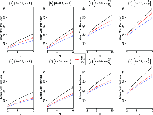
Figure 7: Mean total per period cost over 100 simulations for different forecasting methods and different values of $q$, $\nu$ and $\theta$. Plots (a)–(d) use the 2008 test set and plots (e)–(h) use 2007 as the test set. The vertical lines represent $\pm$1 standard deviation.

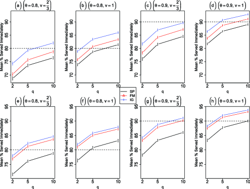
Figure 8: Mean percentage served immediately for the entire test set over 100 simulations for different forecasting methods and different values of $q$, $\nu$ and $\theta$. Plots (a)–(d) use the 2008 test set and plots (e)–(h) use 2007 as the test set. The vertical lines represent $\pm$1 standard deviation.

The mean percentage of callers served immediately can be found in Figure 8. The total number of server hours $\sum\hat{s}_{t}$ used was also recorded for each model for each set of parameter values. A table containing the values of all these quantities can be found in the online supplemental material. Both mean percentage served immediately and mean hourly cost increase with $q$. For each test year, for each level of $(q,\nu,\theta)$, $\sum_{t}\hat{s}_{t}$ differed by between one and three thousand server-hours, for the different models.

5 Conclusions

Our analysis was motivated by a data set provided by Toronto EMS. The proposed forecasting method allows parsimonious modeling of the dependent and nonstationary count-valued EMS call arrival process. Our method is straightforward to implement and demonstrates substantial improvements in forecast performance relative to simpler forecasting methods. We measured the impact of our successive refinements to the model, showing the merit of factor model estimation with covariates and smoothing splines. The factor model was able to capture the nonstationary behavior exhibited in call arrivals. Introduction of the CIIR process allowed adaptive forecasts of deviations from this diurnal pattern.

Assessing the impact that different arrival rate forecasts can have on call centers and related applications has received very little attention in the literature. Our data-based simulation approach is straightforward to implement, and was able to clearly distinguish the effectiveness of each forecasting method. The simulation results coincide with the out-of-sample RMSE analysis in Section 4.3 and provide a practical measure of forecast performance. Relative operating cost is a natural metric for measuring call arrival rate forecasts, and our implementation may easily be extended to many customized cost functions and a wide variety of applications.

Ultimately, we seek to strengthen emergency medical service by improving upon relevant statistical methodology. Future work will consider inclusion of additional covariates and study of other nonlinear time series models. Bayesian methods which directly model count-valued observations have desirable properties for inference and many applications, and are under study. Spatial and spatial–temporal analysis of call arrivals will also offer new benefits to EMS.

References

- Andrews and Cunningham (1995) {barticle}[auto:STB—2010-11-18—09:18:59] \bauthor\bsnmAndrews, \bfnmB.\binitsB. and \bauthor\bsnmCunningham, \bfnmS.\binitsS. (\byear1995). \btitleLL Bean improves call-center forecasting. \bjournalInterfaces \bvolume25 \bpages1–13. \endbibitem
- Andrews and Parsons (1993) {barticle}[auto:STB—2010-11-18—09:18:59] \bauthor\bsnmAndrews, \bfnmB.\binitsB. and \bauthor\bsnmParsons, \bfnmH.\binitsH. (\byear1993). \btitleEstablishing telephone-agent staffing levels through economic optimization. \bjournalInterfaces \bvolume23 \bpages14–20. \endbibitem
- Bianchi, Jarrett and Choudary Hanumara (1998) {barticle}[auto:STB—2010-11-18—09:18:59] \bauthor\bsnmBianchi, \bfnmL.\binitsL., \bauthor\bsnmJarrett, \bfnmJ.\binitsJ. and \bauthor\bsnmChoudary Hanumara, \bfnmR.\binitsR. (\byear1998). \btitleImproving forecasting for telemarketing centers by ARIMA modeling with intervention. \bjournalInternat. J. Forecasting \bvolume14 \bpages497–504. \endbibitem
- Borchers et al. (1997) {barticle}[auto:STB—2010-11-18—09:18:59] \bauthor\bsnmBorchers, \bfnmD.\binitsD., \bauthor\bsnmBuckland, \bfnmS.\binitsS., \bauthor\bsnmPriede, \bfnmI.\binitsI. and \bauthor\bsnmAhmadi, \bfnmS.\binitsS. (\byear1997). \btitleImproving the precision of the daily egg production method using generalized additive models. \bjournalCanad. J. Fisheries and Aquatic Sciences \bvolume54 \bpages2727–2742. \endbibitem
- Brown et al. (2005) {barticle}[mr] \bauthor\bsnmBrown, \bfnmLawrence\binitsL., \bauthor\bsnmGans, \bfnmNoah\binitsN., \bauthor\bsnmMandelbaum, \bfnmAvishai\binitsA., \bauthor\bsnmSakov, \bfnmAnat\binitsA., \bauthor\bsnmShen, \bfnmHaipeng\binitsH., \bauthor\bsnmZeltyn, \bfnmSergey\binitsS. and \bauthor\bsnmZhao, \bfnmLinda\binitsL. (\byear2005). \btitleStatistical analysis of a telephone call center: A queueing-science perspective. \bjournalJ. Amer. Statist. Assoc. \bvolume100 \bpages36–50. \biddoi=10.1198/016214504000001808, mr=2166068 \endbibitem
- Channouf et al. (2007) {barticle}[auto:STB—2010-11-18—09:18:59] \bauthor\bsnmChannouf, \bfnmN.\binitsN., \bauthor\bsnmL’Ecuyer, \bfnmP.\binitsP., \bauthor\bsnmIngolfsson, \bfnmA.\binitsA. and \bauthor\bsnmAvramidis, \bfnmA.\binitsA. (\byear2007). \btitleThe application of forecasting techniques to modeling emergency medical system calls in Calgary, Alberta. \bjournalHealth Care Management Science \bvolume10 \bpages25–45. \endbibitem
- Cox and Isham (1980) {bbook}[mr] \bauthor\bsnmCox, \bfnmDavid Roxbee\binitsD. R. and \bauthor\bsnmIsham, \bfnmValerie\binitsV. (\byear1980). \btitlePoint Processes. \bpublisherChapman & Hall, \baddressLondon. \bidmr=0598033 \endbibitem
- Daskalov (1999) {barticle}[auto:STB—2010-11-18—09:18:59] \bauthor\bsnmDaskalov, \bfnmG.\binitsG. (\byear1999). \btitleRelating fish recruitment to stock biomass and physical environment in the Black Sea using generalized additive models. \bjournalFisheries Research \bvolume41 \bpages1–23. \endbibitem
- Ferland, Latour and Oraichi (2006) {barticle}[mr] \bauthor\bsnmFerland, \bfnmRené\binitsR., \bauthor\bsnmLatour, \bfnmAlain\binitsA. and \bauthor\bsnmOraichi, \bfnmDriss\binitsD. (\byear2006). \btitleInteger-valued GARCH process. \bjournalJ. Time Ser. Anal. \bvolume27 \bpages923–942. \biddoi=10.1111/j.1467-9892.2006.00496.x, mr=2328548 \endbibitem
- Fokianos, Rahbek and Tjøstheim (2009) {barticle}[mr] \bauthor\bsnmFokianos, \bfnmKonstantinos\binitsK., \bauthor\bsnmRahbek, \bfnmAnders\binitsA. and \bauthor\bsnmTjøstheim, \bfnmDag\binitsD. (\byear2009). \btitlePoisson autoregression. \bjournalJ. Amer. Statist. Assoc. \bvolume104 \bpages1430–1439. \biddoi=10.1198/jasa.2009.tm08270, mr=2596998 \endbibitem
- Goldberg (2004) {barticle}[auto:STB—2010-11-18—09:18:59] \bauthor\bsnmGoldberg, \bfnmJ. B.\binitsJ. B. (\byear2004). \btitleOperations research models for the deployment of emergency services vehicles. \bjournalEMS Management J. \bvolume1 \bpages20–39. \endbibitem
- Gross and Harris (1998) {bbook}[mr] \bauthor\bsnmGross, \bfnmDonald\binitsD. and \bauthor\bsnmHarris, \bfnmCarl M.\binitsC. M. (\byear1998). \btitleFundamentals of Queueing Theory, \bedition3rd ed. \bpublisherWiley, \baddressNew York. \bidmr=1600527 \endbibitem
- Gu (1992) {barticle}[auto:STB—2010-11-18—09:18:59] \bauthor\bsnmGu, \bfnmC.\binitsC. (\byear1992). \btitleCross-validating non-Gaussian data. \bjournalJ. Comput. Graph. Statist. \bvolume1 \bpages169–179. \endbibitem
- Gu (2010) {bmisc}[auto:STB—2010-11-18—09:18:59] \bauthor\bsnmGu, \bfnmC.\binitsC. (\byear2010). \bhowpublishedgss: General smoothing splines. R Package Version 1.1-3. \endbibitem
- Harrison, Zeevi and Shum (2005) {barticle}[auto:STB—2010-11-18—09:18:59] \bauthor\bsnmHarrison, \bfnmJ.\binitsJ., \bauthor\bsnmZeevi, \bfnmA.\binitsA. and \bauthor\bsnmShum, \bfnmS.\binitsS. (\byear2005). \btitleA method for staffing large call centers based on stochastic fluid models. \bjournalManufacturing & Service Operations Management \bvolume7 \bpages20–36. \endbibitem
- Hastie (2009) {bmisc}[auto:STB—2010-11-18—09:18:59] \bauthor\bsnmHastie, \bfnmT.\binitsT. (\byear2009). \bhowpublishedgam: Generalized additive models. R Package Version 1.01. \endbibitem
- Hastie and Tibshirani (1990) {bbook}[mr] \bauthor\bsnmHastie, \bfnmT. J.\binitsT. J. and \bauthor\bsnmTibshirani, \bfnmR. J.\binitsR. J. (\byear1990). \btitleGeneralized Additive Models. \bseriesMonographs on Statistics and Applied Probability \bvolume43. \bpublisherChapman & Hall, \baddressLondon. \bidmr=1082147 \endbibitem
- Hastie and Tibshirani (1993) {barticle}[mr] \bauthor\bsnmHastie, \bfnmTrevor\binitsT. and \bauthor\bsnmTibshirani, \bfnmRobert\binitsR. (\byear1993). \btitleVarying-coefficient models. \bjournalJ. Roy. Statist. Soc. Ser. B \bvolume55 \bpages757–796. \bidmr=1229881 \endbibitem
- Henderson (2005) {binproceedings}[auto:STB—2010-11-18—09:18:59] \bauthor\bsnmHenderson, \bfnmS. G.\binitsS. G. (\byear2005). \btitleShould we model dependence and nonstationarity, and if so how? In \bbooktitleProceedings of the 37th Conference on Winter Simulation (\beditorM. Kuhl, N. Steiger, F. Armstrong and J. Joines, eds.) \bpages120–129. \bpublisherIEEE, \baddressPiscataway, NJ. \endbibitem
- Henderson (2009) {bincollection}[auto:STB—2010-11-18—09:18:59] \bauthor\bsnmHenderson, \bfnmS. G.\binitsS. G. (\byear2009). \btitleOperations research tools for addressing current challenges in emergency medical services. In \bbooktitleWiley Encyclopedia of Operations Research and Management Science (\beditorJ. J. Cochran, ed.). \bpublisherWiley, \baddressNew York. \endbibitem
- Kolesar and Green (1998) {barticle}[auto:STB—2010-11-18—09:18:59] \bauthor\bsnmKolesar, \bfnmP.\binitsP. and \bauthor\bsnmGreen, \bfnmL.\binitsL. (\byear1998). \btitleInsights on service system design from a normal approximation to Erlang’s delay formula. \bjournalProduction and Operations Management \bvolume7 \bpages282–293. \endbibitem
- Lopes and West (2004) {barticle}[mr] \bauthor\bsnmLopes, \bfnmHedibert Freitas\binitsH. F. and \bauthor\bsnmWest, \bfnmMike\binitsM. (\byear2004). \btitleBayesian model assessment in factor analysis. \bjournalStatist. Sinica \bvolume14 \bpages41–67. \bidmr=2036762 \endbibitem
- Matteson and Tsay (2011) {bmisc}[auto:STB—2010-11-18—09:18:59] \bauthor\bsnmMatteson, \bfnmD. S.\binitsD. S. and \bauthor\bsnmTsay, \bfnmR. S.\binitsR. S. (\byear2011). \bhowpublishedConstrained independent component analysis. Unpublished manuscript. \endbibitem
- McCullagh and Nelder (1989) {bbook}[mr] \bauthor\bsnmMcCullagh, \bfnmP.\binitsP. and \bauthor\bsnmNelder, \bfnmJ. A.\binitsJ. A. (\byear1989). \btitleGeneralized Linear Models, \bedition2nd ed. \bpublisherChapman & Hall, \baddressLondon. \endbibitem
- Opsomer, Wang and Yang (2001) {barticle}[mr] \bauthor\bsnmOpsomer, \bfnmJean\binitsJ., \bauthor\bsnmWang, \bfnmYuedong\binitsY. and \bauthor\bsnmYang, \bfnmYuhong\binitsY. (\byear2001). \btitleNonparametric regression with correlated errors. \bjournalStatist. Sci. \bvolume16 \bpages134–153. \biddoi=10.1214/ss/1009213287, mr=1861070 \endbibitem
- Pierce and Schafer (1986) {barticle}[mr] \bauthor\bsnmPierce, \bfnmDonald A.\binitsD. A. and \bauthor\bsnmSchafer, \bfnmDaniel W.\binitsD. W. (\byear1986). \btitleResiduals in generalized linear models. \bjournalJ. Amer. Statist. Assoc. \bvolume81 \bpages977–986. \bidmr=0867620 \endbibitem
- R Development Core Team (2009) {bmisc}[auto:STB—2010-11-18—09:18:59] \borganizationR Development Core Team (\byear2009). \bhowpublishedR: A Language and Environment for Statistical Computing. R Foundation for Statistical Computing, Vienna, Austria. \endbibitem