Bayesian hierarchical modeling for temperature reconstruction from geothermal data

Abstract

We present a Bayesian hierarchical modeling approach to paleoclimate reconstruction using borehole temperature profiles. The approach relies on modeling heat conduction in solids via the heat equation with step function, surface boundary conditions. Our analysis includes model error and assumes that the boundary conditions are random processes. The formulation also enables separation of measurement error and model error. We apply the analysis to data from nine borehole temperature records from the San Rafael region in Utah. We produce ground surface temperature histories with uncertainty estimates for the past 400 years. We pay special attention to use of prior parameter models that illustrate borrowing strength in a combined analysis for all nine boreholes. In addition, we review selected sensitivity analyses.

and Jenny Brynjarsdottir, L. Mark Berliner T1Supported by NSF Grant ATM-07-24403.

1 Introduction

Reconstruction of past climate plays an important role in climate change analysis. Comparisons between climate behavior before and after human influences are a relevant component of claims of attribution of climate change to our activities. The term paleoclimate is used in reference to data analysis and modeling of climate for times before the modern era of data collection. The time periods of interest range from hundreds to millions of years before the present. Of course, as our interest moves toward the past, the availability of reliable and spatially and temporally plentiful observations of weather and climate diminishes. In response, scientists have developed the use of proxy indicators of climate [Jansen et al. (2007)].

A proxy is a quantity taking values that respond to climate behavior. For example, annual tree ring thicknesses respond to weather variables that control growth, that is, temperature and precipitation. If one develops useful models for proxies as rough functions of climate, then the models can be inverted to estimate climate behavior based on observed proxy variables. The statistical notions of regression and inverse regression analyses are immediately evident. Though exceptions exist and the trend is positive [e.g., Haslett et al. (2006); Li, Nychka and Ammann (2007, 2010)], there has been insufficient participation by statisticians in paleoclimate reconstruction. This is surprising in view of the richness of the statistical challenges: proxies are themselves observed with error; the forward models for proxies as functions of climate are partially known at best and subject to model errors; inverse analyses are not trivial statistically; spatial and temporal coverage and mismatches between proxy data sets and desired climate inferences are among the issues. Furthermore, there is substantial interest in paleoclimate among policy makers and the general public [Wegman, Scott and Said (2006); Smith, Berliner and Guttorp (2010)].

In this article we focus on the critical problem of surface temperature reconstruction [Jansen et al. (2007); North et al. (2006)]. We analyze borehole temperature data sets and their use in reconstructing surface temperature time series [e.g., Beltrami and Mareschal (1995); Pollack, Huang and Shen (1998)]. A borehole is a narrow shaft drilled into the ground (or ice), typically vertically, in search of subterranean resources (gas, oil, water, minerals, etc.). Boreholes are also used to monitor environmental processes (e.g., percolation of contaminants) or as pilots to access suitability for more intense drilling or construction projects. Borehole data that are used for temperature reconstruction are typically obtained as byproducts of such projects. Therefore, borehole data are observations of opportunity rather than having been designed with climate reconstruction in mind. We note that borehole data are temperature measurements, and, hence, perhaps not as indirect a measure of surface temperature as other proxies. However, the problems of developing and inverting a model for borehole data as a function of surface temperatures are challenging.

The underlying theory for using borehole data to infer surface temperature is the physics of heat conduction. In principle, the transfer of heat is governed by the heat equation. This is a partial differential equation describing the temporal evolution of the temperature field over some domain. The idea is that the surface temperatures over time serve as boundary conditions for the evolution of temperature below the surface. Then information regarding subsurface temperatures can be inverted to estimate the boundary conditions.

There are important issues and uncertainties that arise in applying this strategy. First, subsurface temperatures respond to ground-surface temperatures as opposed to near surface air temperatures. Though the latter two are related, they are not identical, perhaps due to snow cover and other factors. Next, as heat conducts into deepening levels of the subsurface, it spreads or smears out, leading to losses in information regarding the boundary as time increases. Though this problem is well known, we will seek explicit characterizations of this loss of information as reflected in uncertainty measures associated with our results. Another issue is that there are factors affecting heat conduction that are difficult to quantify. For example, conduction rates depend on characteristics of the media (i.e., rock types) through which the heat flows. Further, percolation of water through the media also impacts heat flow. For such reasons, we incorporate the heat equation with error and unknown parameters in our modeling.

We present Bayesian modeling and analysis for data from 9 boreholes in the San Rafael region in Utah. To combine information from these boreholes, we assume model parameters are site-specific, but sampled from common distributions. Our modeling incorporates both the observations and physics into an analysis that is sensitive to the uncertainties in both information sources. The use of such physical-statistical analyses in geophysical problems is increasing; for examples, see Berliner (2003), Berliner et al. (2008) and Wikle et al. (2001). See Hopcroft, Gallagher and Pain (2007) for a related Bayesian analysis of borehole data.

1.1 Review: Borehole data analysis

The conventional approach is to frame analyses in terms of reduced temperatures defined as follows. For a given borehole, consider $N$ depths $z_{1},\ldots,z_{N}$, where increasing values of $z$ correspond to increasing depths. Let $\mathbf{T}$ be the $N\times 1$ vector of true temperatures at these depths. The corresponding vector of reduced temperatures is given by

$$\mathbf{T}_{r}=\mathbf{T}-T_{0}\mathbf{1}-q_{0}\mathbf{R},\vspace*{-2pt}$$ (1)

where $T_{0}$ is the surface temperature intercept, $\mathbf{1}$ is an $N\times 1$ vector whose elements are all equal to one, $q_{0}$ represents background heat flow, and $\mathbf{R}$ is an $N\times 1$ vector of thermal resistances at each of the depths. This modeling step is intended to account for the fact that both heating from the earth’s core and rates of heat conduction vary with depth, thereby justifying use of the simple heat equation model described in Section 3.1.

The thermal resistances account for differences in heat conduction and are assumed known throughout the analysis (see Section 2). To deal with the unknowns $T_{0}$ and $q_{0}$, it is customary to replace the true temperatures $\mathbf{T}$ by the observed temperatures, $\mathbf{Y}$, in (1). Then, $T_{0}$ and $q_{0}$ are estimated via least squares by regressing $\mathbf{Y}$ onto $\mathbf{R}$. In that step a subset of the data is used, corresponding to those depths where the climate change signal is assumed to be negligible [for our data this means below 150 m or 200 m, depending on the region; Harris and Chapman (1995)]. The resulting estimates

$$\hat{T}_{r}(z_{i})=Y(z_{i})-\bigl{(}\hat{T}_{0}+\hat{q}_{0}R(z_{i})\bigr{)},\qquad i=1,\ldots,N,$$ (2)

are then treated as the true reduced temperatures.

Having made the above adjustments, the heat equation is assumed to apply. Let $\mathbf{T}_{h}$ be a $K\times 1$ surface temperature history vector. Here, the surface temperatures are assumed to be constants over $K$ time intervals used in the analysis. The heat equation can be solved (see Section 3), leading to the linear relationship

$$\hat{\mathbf{T}}_{r}=A\mathbf{T}_{h},$$ (3)

where $A$ is an $N\times K$ matrix developed from the solution to the heat equation [see (10)]. The objective then is to solve the inverse problem, that is, obtain an estimate of $\mathbf{T}_{h}$. In most examples, $A$ is ill-conditioned and the inversion of $A^{\prime}A$ is unstable. Therefore, traditional regression methods which involve taking the inverse of $A^{\prime}A$ lead to unstable estimates of $\mathbf{T}_{h}$. A common approach is to use a singular value decomposition (SVD) of the $A$ matrix and retain only a few of the singular vectors [Vasseur et al. (1983); Beltrami and Mareschal (1991); Mareschal and Beltrami (1992); Harris and Chapman (1995)]. In this paper we take a hierarchical Bayesian regression approach that does not involve taking the inverse of $A^{\prime}A$. Hence, we avoid having to pick the number of singular vectors (principal components) to retain.

Other approaches can be found in the geophysical literature. For example, functional space inversion is a popular method [Shen and Beck (1991, 1992); Harris and Chapman (1998)]. A comparative study of some inverse methods in this setting can be found in Shen et al. (1992).

1.2 Outline

The paper is organized as follows. In Section 2 we describe the borehole data used in the analysis. In Section 3 after a brief introduction to the physical model the analysis is based on, we develop a Bayesian hierarchical model. To best convey the ideas, we first present a single-site borehole model in Section 3.2. We extend it to include data from multiple boreholes in Section 3.3. The results are presented in Section 4. In Section 4.2 we compare the results to those of single-site models and in Section 4.3 we present a number of sensitivity analysis. We end with a discussion in Section 5.

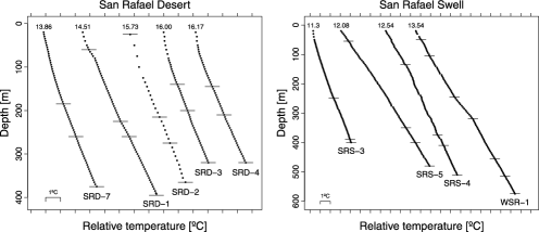
Figure 1: Measured temperature-depth profiles from boreholes in the San Rafael Desert (left) and the San Rafael Swell (right). The temperatures are shifted so they do not overlap, one tick on the x axis corresponds to $1^{\circ}$C. The value of the shallowest measurement is shown above each profile. The horizontal line segments show the formation boundaries, the names of the formations are given in Table 1.

2 Data

We consider borehole data from the Colorado Plateau in Utah. The data consist of nine measured temperature-depth profiles (shown in Figure 1) belonging to two regions, the San Rafael Desert and the San Rafael Swell. The geography of these regions is characterized by layered sedimentary rocks that each have different thermal conductivities. Measurements of these different conductivities are available [Bodell and Chapman (1982)] and have been adjusted to the specific formations in the boreholes used in this analysis so that the estimated thermal conductivity for each formation may be different between regions but not within regions [see Harris and Chapman (1995) for details about these adjustments]. The adjusted thermal conductivities ($k$) for each sedimentary formation and abbreviated formation names are shown in Table 1 along with the formation boundaries within each borehole. For definitions of the abbreviated formation names see Bodell and Chapman (1982). The sedimentary formation boundaries are also shown as small horizontal line segments in Figure 1. For more background on the data and temperature reconstructions based on them see Harris and Chapman (1995, 1998).

Thermal resistance ($R$) is a function of depth and the thermal conductivity at that depth, and is calculated as

$$R(z_{i})=\sum_{l=1}^{i}\frac{z_{l}-z_{l-1}}{k(z_{l})},\qquad i=1,\ldots,N,$$ (4)

where $k(z_{l})$ is the conductivity for the depth interval from $z_{l-1}$ to $z_{l}$. Recall that $z_{0}=0$ denotes the surface and $z$ is increasing in depth. If the conductivity is constant ($k$) for the entire borehole, (4) reduces to $R(z_{i})=z_{i}/k$, that is, a constant temperature gradient.

=300pt Borehole Depth [m] Formation $\bolds k$ [W/mK] San Rafael Desert SRD-1 60 Jca 2.91 $\hat{T}_{0}=13.72$ 225 Jna 4.09 year: 1979 260 JTrk 3.96 395 Trwi 3.86 SRD-2 25 Jca 2.91 $\hat{T}_{0}=15.12$ 215 Jna 4.09 year: 1976 275 JTrk 3.96 365 Trwi 3.86 SRD-3 140 Jna 4.09 $\hat{T}_{0}=15.38$ 200 JTrk 3.96 year: 1979 320 Trwi 3.86 SRD-4 145 Jna 4.09 $\hat{T}_{0}=15.51$ 210 JTrk 3.96 year: 1979 320 Trwi 3.86 SRD-7 185 Jna 4.09 $\hat{T}_{0}=13.16$ 260 JTrk 3.96 year: 1980 375 Trwi 3.86 San Rafael Swell SRS-3 250 Pco 5.01 $\hat{T}_{0}=10.76$ 390 Pec 4.35 year: 1979 400 Mr 4.82 SRS-4 135 Jca 2.91 $\hat{T}_{0}=11.82$ 375 Jna 4.18 year: 1979 410 JTrk 3.86 510 Trwi 4.17 SRS-5 55 Jca 2.91 $\hat{T}_{0}=11.82$ 350 Jna 4.18 year: 1979 400 JTrk 3.86 480 Trwi 4.17 WSR-1 50 Js 4.10 $\hat{T}_{0}=12.87$ 105 Jcu 3.96 year: 1980 245 Je 3.43 320 Jca 2.91 455 Jna 4.18 515 JTrk 3.86 575 Trwi 4.17

Table 1: Depth to formation boundaries within each borehole, names of the formation types down to each boundary and the corresponding thermal conductivities ($k$). The table also shows for each borehole the estimated surface temperature intercept, $\hat{T}_{0}$, and the year the borehole was logged

3 Bayesian hierarchical model

3.1 Physics based modeling

Following convention, we assume that for reduced temperatures, boreholes are well approximated as homogeneous, heat source free (except at the surface), one-dimensional, semi-infinite solids (i.e., a single boundary is at the surface). It follows that the reduced temperatures, $T_{r}(z,t)$ at depth $z$ and time $t$, can be reasonably modeled by the heat equation,

$$\frac{\partial^{2}T_{r}(z,t)}{\partial z^{2}}=\frac{1}{\kappa}\,\frac{\partial T_{r}(z,t)}{\partial t},$$ (5)

where $\kappa$ is the thermal diffusivity of rock. As is customary in borehole analysis, we fix $\kappa$ to be $10^{-6}$ m²/s [see, e.g., Harris and Chapman (1995)]. The boundary condition, $T_{r}(0,t)$, is the primary target of our inference. Assuming that the initial reduced temperatures, $T_{r}(z,t_{1})$, are zero for all depths $z$, the solution to (5) is

$$T_{r}(z,t)=\frac{2}{\sqrt{\pi}}\int_{z/2\sqrt{\kappa t}}^{\infty}T_{r}\biggl{(}0,t-\frac{z^{2}}{4\kappa\mu^{2}}\biggr{)}e^{-\mu^{2}}\,d\mu$$ (6)

[e.g., Carlslaw and Jaeger (1959)]. We assume that the boundary function is a step function,

$$T_{r}(0,t)=\cases{\displaystyle T_{1},&\quad if $t_{1}<t<t_{2}$,\cr\displaystyle T_{2},&\quad if $t_{2}<t<t_{3}$,\cr\displaystyle\vdots\cr\displaystyle T_{K},&\quad if $t_{K}<t<t_{K+1}$.}$$ (7)

Then the solution (6) reduces to

$$T_{r}(z,t) = T_{1}\mathrm{erfc}\biggl{(}\frac{z}{\sqrt{4\kappa(t-t_{1})}}\biggr{)}+(T_{2}-T_{1})\mathrm{erfc}\biggl{(}\frac{z}{\sqrt{4\kappa(t-t_{2})}}\biggr{)}$$

$${}+\cdots+(T_{K}-T_{K-1})\mathrm{erfc}\biggl{(}\frac{z}{\sqrt{4\kappa(t-t_{K})}}\biggr{)},$$

where $\mathrm{erfc}(\cdot)$ is the complementary error function

$$\mathrm{erfc}(x)=\frac{2}{\sqrt{\pi}}\int_{x}^{\infty}e^{-\mu^{2}}\,d\mu.$$ (9)

Here, the time points $t_{1},\ldots,t_{K+1}$ are calendar years, $t_{1}$ being the earliest year considered and $t_{K+1}$ is the year the borehole data were collected. For example, borehole SRD-7 was logged in $t_{12}=1980$ and we selected the following years for the time points $t_{1},\ldots,t_{11}$: 1600, 1650, 1700, 1750, 1800, 1850, 1875, 1900, 1925, 1950 and 1965. This range is in concert with other analyses. We also performed some analyses using a slightly more refined temporal grid. These resulted in little change in the general form of the posterior results. We note that for highly refined grids, the structure and dimension of $A$ becomes an issue.

Collecting terms in (3.1), we can write the solution at $t=t_{K+1}$ in vector form:

$$\mathbf{T}_{r}=A\mathbf{T}_{h},$$ (10)

where $\mathbf{T}_{r}=(T_{r}(z_{1},t_{K+1}),\ldots,T_{r}(z_{N},t_{K+1}))^{\prime}$, $\mathbf{T}_{h}=(T_{1},\ldots,T_{K})^{\prime}$, and $A$ is an $N\times K$ matrix with $(i,j)$th entry

$$\mathrm{erfc}\biggl{(}\frac{z_{i}}{\sqrt{4\kappa(t_{K+1}-t_{j})}}\biggr{)}-\mathrm{erfc}\biggl{(}\frac{z_{i}}{\sqrt{4\kappa(t_{K+1}-t_{j+1})}}\biggr{)}$$

for $i=1,\ldots,N$ and $j=1,\ldots,K-1$ and $(i,K)$th entry

$$\mathrm{erfc}\biggl{(}\frac{z_{i}}{\sqrt{4\kappa(t_{K+1}-t_{K})}}\biggr{)};\qquad i=1,\ldots,N.$$

3.2 Single-site model

It is useful to view the modeling in three basic stages, a data model, process model and a parameter model.

(i) Data model. Let $\mathbf{Y}$ be a vector of observed temperatures at depths $z_{1},\ldots,z_{N}$ and let $\mathbf{T}$ denote the $N$-dimensional vector of corresponding true temperatures. We assume that the observations are noisy, unbiased measurements of the true temperatures. Specifically, we assume that

$$\mathbf{Y}=\mathbf{T}+\bolds\varepsilon,$$ (11)

where $\bolds\varepsilon$ is an $N$-dimensional vector of normally distributed, independent errors, all with mean zero and common variance $\sigma_{Y}^{2}$ (see Section 4.3.4 for discussion of the independence assumption).

Recalling the definition of reduced temperatures in (1), the true temperatures can be written as

$$\mathbf{T}=\mathbf{T}_{r}+T_{0}\mathbf{1}_{N}+q_{0}\mathbf{R},$$ (12)

where $\mathbf{T}_{r}$ is the vector of true reduced temperatures and other quantities are defined after (1).

Combining (11) and (12), the assumed data model is the conditional distribution

$$\mathbf{Y}|\mathbf{T}_{r},q_{0},\sigma_{Y}^{2}\sim N(\mathbf{T}_{r}+T_{0}\mathbf{1}_{N}+q_{0}\mathbf{R},\sigma_{Y}^{2}I_{N}),$$ (13)

where the vertical bar $|$ is read “given,” $\sim$ is read “is distributed,” and $I_{N}$ is the $N\times N$ identity matrix.

Note that $T_{0}$ and $\mathbf{T}_{r}$ in (13) are not identifiable in that, for any constant $c$, the shifted parameters $\mathbf{T}_{r}\rightarrow\mathbf{T}_{r}+c\mathbf{1}_{N}$, $T_{0}\rightarrow T_{0}-c$ yield identical data models. To circumvent this issue, we assume that $T_{0}$ is known. The assumed values of $T_{0}$ for the boreholes analyzed here are given in Table 1. We report on the sensitivity of results to the choice of $T_{0}$ in Section 4.3.1.

(ii) Process model. We let $\mathbf{T}_{h}$ denote the $K$-vector containing the surface temperature history. We incorporate the heat equation in defining a stochastic process model

$$\mathbf{T}_{r}|\mathbf{T}_{h},\Sigma\sim N(A\mathbf{T}_{h},\Sigma)$$ (14)

[recall (10)]. We also assume a Gaussian prior for the histories:

$$\mathbf{T}_{h}\sim N(\bolds\mu,\Gamma).$$ (15)

(iii) Parameter model. We assume that the covariance matrix of the process model errors [see (14)] is diagonal with common variance, namely, $\Sigma=\sigma^{2}I_{N}$. That is, after accounting for the dependence on the temperature history, the heat equation offers reliable explanation of reduced temperatures requiring only some local-in-depth errors. In Section 4.3.4 we consider sensitivity of results with respect to the independence assumption.

Additional specifications of parameter priors is delayed until we discuss modeling for multiple sites.

3.3 Multiple-site model: Spatially distributed parameters

We extend the model to combine data from multiple boreholes by allowing site-specific processes and parameters. A list of all the model parameters used in this model is provided in Appendix A.

(i) Data model. We assume that measurements from different sites are conditionally independent with data models that depend only on site-specific processes and parameters. We also assume that reduced temperature vectors from different sites are conditionally independent with priors that depend on site-specific histories and parameters. Formally, the data model is the product of densities corresponding to the models

$$\mathbf{Y}_{j}|\mathbf{T}_{rj},q_{0j},\sigma_{Y_{j}}^{2}\sim N_{N_{j}}(\mathbf{T}_{rj}+T_{0j}\mathbf{1}_{N_{j}}+q_{0j}\mathbf{R}_{j},\sigma_{Y_{j}}^{2}I_{N_{j}})$$ (16)

for the 9 sites labeled $j=1,\ldots,9$ with observation vectors of length $N_{j}$.

(ii) Process model. Similarly, the process model for the reduced temperature vectors is the product of densities for

$$\mathbf{T}_{rj}|\mathbf{T}_{hj},\sigma_{j}^{2}\sim N_{N_{j}}(A_{j}\mathbf{T}_{hj},\sigma_{j}^{2}I_{N_{j}}).$$ (17)

Since all 9 sites are in the Colorado Plateau, we expect them to have been influenced by common large-scale climate effects. However, the sites are located in two subregions: Sites 1–5 are in the San Rafael Desert (D), Sites 6–9 are in the San Rafael Swell (S). To account for common influences within subregions, we assume that all 9 histories are conditionally independent, with parameters depending on subregions:

$$\mathbf{T}_{hj}|\bolds\mu_{D},\gamma_{D}^{2}\sim N_{K}(\bolds\mu_{D},\gamma_{D}^{2}I_{K}),\qquad j=1,\ldots,5,$$ (18)

and

$$\mathbf{T}_{hj}|\bolds\mu_{S},\gamma_{S}^{2}\sim N_{K}(\bolds\mu_{S},\gamma_{S}^{2}I_{K}),\qquad j=6,\ldots,9.$$ (19)

We remark that this is a very elementary spatial model. More complex spatial modeling of parameters is feasible and recommended, depending on prior information and data richness.

(iii) Parameter model.

Model for heat flow parameters: To account for region-wide influences, we assume that the heat flow parameters $\mathbf{q}=(q_{01},\ldots,q_{09})^{\prime}$ are sampled from priors with dependence structures. These priors are similar to exchangeable models [e.g., Section 4.6.2 in Berger (1985)].

The heat flow parameters are assumed to be conditionally independent with Gaussian priors where both the mean and the variance depend on which region the borehole is in,

$$q_{0j}|\nu_{D},\tau_{D}^{2}\sim N(\nu_{D},\tau_{D}^{2}),\qquad j=1,\ldots,5,$$ (20)

and

$$q_{0j}|\nu_{S},\tau_{S}^{2}\sim N(\nu_{S},\tau_{S}^{2}),\qquad j=6,\ldots,9.$$ (21)

The means $\nu_{D}$ and $\nu_{S}$ are assumed to be a priori independent with Gaussian priors having common mean $\nu$:

$$\nu_{D}|\nu\sim N(\nu,\eta^{2})\quad\mbox{and}\quad\nu_{S}|\nu\sim N(\nu,\eta^{2}).$$ (22)

Next, we assume that

$$\nu\sim N(\nu_{0},\eta_{0}^{2}).$$ (23)

We can combine the distributions in (22) and (23) and integrate out $\nu$, leading to the following prior for $\nu_{D}$ and $\nu_{S}$:

$$\pmatrix{\displaystyle\nu_{D}\cr\displaystyle\nu_{S}}\sim N\left(\pmatrix{\displaystyle\nu_{0}\cr\displaystyle\nu_{0}},\pmatrix{\displaystyle\eta^{2}_{D}+\eta^{2}_{0}&\eta^{2}_{0}\cr\displaystyle\eta^{2}_{0}&\eta^{2}_{S}+\eta^{2}_{0}}\right).$$ (24)

Model for means of histories: We assume the means of the temperature histories $\bolds\mu_{D}$ and $\bolds\mu_{S}$ in (18) and (19) have common mean $\bolds\mu$; $\bolds\mu_{D}|\bolds\mu\sim N(\bolds\mu,\sigma_{D}^{2}I_{K})$ and $\bolds\mu_{S}|\bolds\mu\sim N(\bolds\mu,\sigma_{S}^{2}I_{K})$. We in turn assume that $\bolds\mu\sim N(\bolds\mu_{0},\break\sigma_{0}^{2}I_{K})$. As in the development of (24), integrating out $\bolds\mu$ yields the following joint prior for $\bolds\mu_{D}$ and $\bolds\mu_{S}$:

$$\pmatrix{\displaystyle\bolds\mu_{D}\cr\displaystyle\bolds\mu_{S}}\sim N\left(\pmatrix{\displaystyle\bolds\mu_{0}\cr\displaystyle\bolds\mu_{0}},\pmatrix{\displaystyle(\sigma^{2}_{D}+\sigma^{2}_{0})I_{K}&\sigma^{2}_{0}I_{K}\cr\displaystyle\sigma^{2}_{0}I_{K}&(\sigma^{2}_{S}+\sigma^{2}_{0})I_{K}}\right).$$ (25)

Note that the covariance structures in (18), (19) and (25) only include some spatial dependence, but no temporal structure. Some spatial-temporal dependence among historical temperature values are displayed in their posterior distribution.

Priors for the variances: The measurement error and process model error variances appearing in (16)–(21) are all assigned independent, inverse gamma priors:

$$\sigma^{2}_{Y_{j}} \sim IG(a_{Y},b_{Y})\quad\mbox{and}\quad\sigma_{j}^{2}\sim IG(a,b)\qquad\mbox{for }j=1,\ldots,9,$$ (26)

$$\tau_{D}^{2} \sim IG(a_{\tau},b_{\tau})\quad\mbox{and}\quad\tau_{S}^{2}\sim IG(a_{\tau},b_{\tau}),$$ (27)

$$\gamma_{D}^{2} \sim IG(a_{\gamma},b_{\gamma})\quad\mbox{and}\quad\gamma_{S}^{2}\sim IG(a_{\gamma},b_{\gamma}).$$ (28)

3.4 Selection of parameters of prior distributions

We describe the selections of parameters of priors or hyperparameters introduced above:

Measurement error variances ($a_{Y},b_{Y}$). As suggested in Harris and Chapman (1995), “The precision and accuracy of the measurements are estimated to be better than 0.01 K and 0.1 K, respectively.” We view this as suggesting that a reasonable prior mean for the variances of the measurement errors, $\sigma^{2}_{Y_{j}}$, $j=1,\ldots,9$, is $0.11^{2}$. A conservative choice for the prior variances is $1.0$. The values $a_{Y}=2.000146$ and $b_{Y}=0.012102$ yield an inverse gamma distribution matching these properties. For additional intuition we remark that the 0.025 and 0.975 quantiles of this prior are equal to $0.002172$ and $0.049955$, respectively. Further, the corresponding 0.025 and 0.975 quantiles for the $\sigma_{Y_{j}}$ are $0.0466$ and $0.2235$, respectively.

Model error variances ($a,b$). Though we know comparatively little about the variances $\sigma_{j}^{2}$ of the model errors, we can develop some plausible expectations. For example, if the standard deviations of the model errors are 0.5, we expect the model to be within $1.5^{\circ}C$ from the truth $99.7\%$ of the time. Hence, we specified the prior mean of each $\sigma_{j}^{2}$ to be $0.50^{2}$ and a very large prior variance of $100$. These selections correspond to $a=2.000625$ and $b=0.250156$. The corresponding 0.025 and 0.975 quantiles for the $\sigma_{j}$ are $0.212$ and $1.016$, respectively.

Heat flow parameters ($\nu_{0},\eta^{2}_{D},\eta^{2}_{S},\eta^{2}_{0},a_{\tau},b_{\tau}$). The background heat flow $q_{0}$ has been shown in other studies to range from about 30 mW/m² (milliwatt per meter-squared) to about 100 mW/m², with the majority of values ranging between 50 and 70 mW/m² [Bodell and Chapman (1982); Beltrami and Mareschal (1995); Dorofeeva, Shen and Shapova (2002), e.g.]. Focusing on (24), we selected the prior mean $\nu_{0}=60$ mW/m² and set the standard deviation $\eta_{0}=20$ mW/m². The standard deviations $\eta_{D}$ and $\eta_{S}$ represent variability due to subregion. We set $\eta_{D}=\eta_{S}=10$. Note that these selections imply that the prior standard deviations of $\nu_{D}$ and $\nu_{S}$ are equal to $(20^{2}+10^{2})^{0.50}\approx 22.36$ mW/m² and the correlation between $\nu_{D}$ and $\nu_{S}$ is $0.80$. We discuss sensitivities of results to these selections in Section 4.3.2.

Recalling (20) and (21), $\tau_{D}^{2}$ and $\tau_{S}^{2}$ quantify variability of the $q_{0j}$ about their regionally defined prior means. We set the prior means for these variances to $0.1^{2}$ with a corresponding large prior variance of 1. It follows that we select $a_{\tau}=2.000100$ and $b_{\tau}=0.010001$. Note that the units here are W/m², so this corresponds to $\tau^{2}_{D}$ and $\tau^{2}_{S}$ having prior mean of $100^{2}$ (mW/m²)² and the 0.025 and 0.975 quantiles for $\tau_{D}$ and $\tau_{S}$ are $42.4$ mW/m² and $203.2$ mW/m², respectively.

Histories ($\bolds\mu_{0},\sigma^{2}_{D},\sigma^{2}_{S},\sigma^{2}_{0},a_{\gamma},b_{\gamma}$). In the model parameterizations used here both reduced temperatures and temperature histories represent departures from the baseline surface temperature $T_{0}$ [see (12)]. Hence, a reasonable prior mean for $\mathbf{T}_{h}$ is $\bolds\mu_{0}=\mathbf{0}$. Further, these departures occur over time intervals of lengths between 10 and 50 years. Focusing on (25), we selected $\sigma^{2}_{0}=0.1$ and $\sigma^{2}_{D}=\sigma^{2}_{S}=0.2$. These selections imply that the prior standard deviations of the coordinated $\mu_{Dk}$ and $\mu_{Sk}$, $k=1,\ldots,K$, are equal to $(0.1+0.2)^{0.50}\approx 0.5477$ and the correlation between $\mu_{Dk}$ and $\mu_{Sk}$ is $0.333$. We discuss sensitivities of results to these selections in Section 4.3.3.

Finally, recalling (18) and (19), $\gamma_{D}^{2}$ and $\gamma_{D}^{2}$ quantify variability of the elements of the history vectors about their regionally defined prior means. We set the prior means for these variances to $0.8$ and prior variances equal to 1. It follows that we select $a_{\gamma}=2.064$ and $b_{\gamma}=0.8512$ and the corresponding 0.025 and 0.975 quantiles for $\gamma_{D}$ and $\gamma_{s}$ are $0.387$ and $1.801$, respectively.

4 Results

4.1 Multiple-site model

The multiple-site model described in Section 3.3 has 818 unknown parameters, including 664 elements of the reduced temperature vectors $\mathbf{T}_{rj}$. We implemented a Gibbs sampler in R to obtain samples from the posterior distribution. The full conditional distributions used are given in Appendix B. We obtained 30,000 samples and discarded the first 2000 as burn-in, leaving 28,000 samples to use for inference. Trace-plots for parameters and a random selection of elements of $\mathbf{T}_{rj}$ showed no indication of convergence problems. We estimated marginal posterior densities using (Gaussian) kernel density estimation.

The ground surface temperature (GST) histories, $\mathbf{T}_{hj}$, are of primary interest. Estimated posterior means and credible sets for the GST histories are shown in Figure 2. In Figure 3 we show 5 samples of $\mathbf{T}_{hj}$ for each borehole. These 5 samples are taken 6000 MCMC iterations apart (after burn-in) and 100 iterations apart between boreholes. Note that the generated realizations are not overly smooth, but that the spreads of the realizations are decreasing as time approaches the present. Estimated posterior means and credible sets for the mean GST histories for the San Rafael (SR) Desert and SR Swell regions, $\bolds\mu_{D}$, $\bolds\mu_{S}$, and prior and posterior densities of the parameters $\gamma_{D}$ and $\gamma_{S}$, are shown in Figure 4. One striking feature of the GST histories is that posterior uncertainties are substantial. We see patterns of warming in the last century (and cooling for site WSR-1), but there are large posterior uncertainties associated with the estimated trends at each borehole. On the other hand, the posterior uncertainty is lower for more recent times (especially at the last time point).

We note that the temperature trends (posterior means) are similar within the SR Desert sites, but quite variable within the SR Swell region, most notably at sites SRS-5 and WSR-1. Furthermore, the posterior credible intervals are wider for boreholes in the SR Swell. This difference is also apparent in the density estimates of the standard deviation of the GST histories: $\gamma_{S}$ is larger than $\gamma_{D}$ (see Figure 4, right). The mean GST histories ${\bolds\mu}_{D}$ and ${\bolds\mu}_{S}$ show slightly different temperature trends (Figure 4, left), but the posterior uncertainty is somewhat large and increasing as we go further back in time.

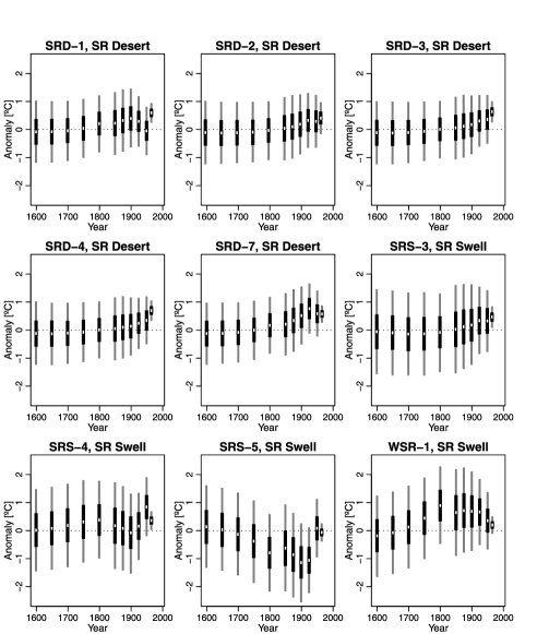
Figure 2: Estimated posterior means and credible sets for the ground surface temperature (GST) histories, $\mathbf{T}_{hj}$. The white squares show the posterior means of $\mathbf{T}_{hj}$ and the vertical bars show symmetric 50% (thicker and black) and 90% (thinner and grey) posterior credible intervals.

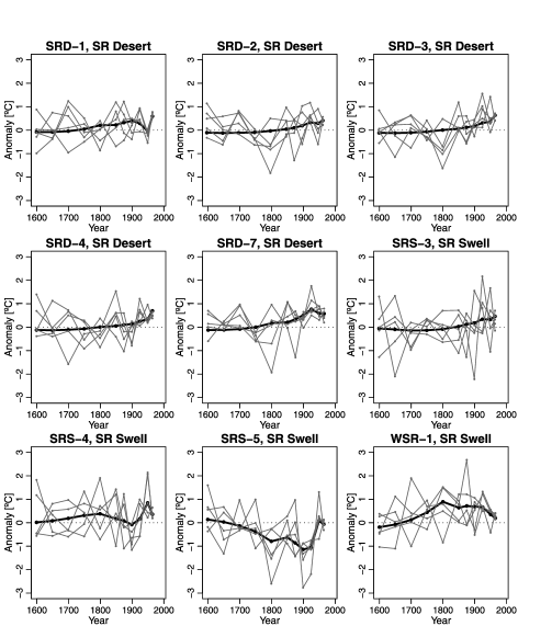
Figure 3: Ensembles of ground surface temperature (GST) histories generated from the posterior distribution. For each borehole, the thick black lines show the posterior means of $\mathbf{T}_{hj}$ and the five grey lines are five different samples of $\mathbf{T}_{hj}$.

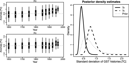
Figure 4: Left: Estimated posterior means (white squares) and symmetric 50% and 90% posterior credible intervals for the mean GST histories $\bolds\mu_{D}$ (upper) and $\bolds\mu_{S}$ (lower). Right: Estimated posterior densities for the standard deviations of the GST histories for both areas, $\gamma_{D}$ and $\gamma_{S}$. The prior density is the same for both $\gamma_{D}$ and $\gamma_{S}$ (dotted line).

Estimated marginal posterior densities of the site-wise measurement and model error standard deviations, $\sigma_{Yj}$ and $\sigma_{j}$, are shown in Figure 5. The locations of these densities are quite different from the prior means. The $\sigma_{Yj}$ are of the order $0.03$–$0.05^{\circ}$C compared to their prior mean $0.11^{\circ}$C. The $\sigma_{j}$ are of the order $0.05$–$0.15^{\circ}$C compared to the prior mean $0.5^{\circ}$C. An interesting pattern emerges in Figure 5. Both $\sigma_{Yj}$ and $\sigma_{j}$ have higher posterior uncertainty for boreholes in the SR Desert than the SR Swell. Note that the boreholes in the SR Swell have more measurements than those in the SR Desert (see Figure 1). The SRD-2 borehole has by far the fewest measurements and, as indicated in Figure 5, densities for $\sigma_{Yj}$ and $\sigma_{j}$ for that site are wider and are closer to the prior than the other densities.

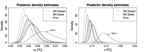
Figure 5: Estimated posterior densities of the measurement error standard deviations $\sigma_{Yj}$ (left) and the model error standard deviations $\sigma_{j}$ (right). In both cases the prior is the same for all nine boreholes (dotted lines).

Estimated posterior densities of the background heat flow $q_{0j}$ are shown in Figure 6. Posterior means and 90% credible intervals for $q_{0j}$ and the means $\nu_{D}$ and $\nu_{S}$ are shown in Table 2. Estimated posterior densities of the means and standard deviations of the heat flow, $\nu_{D}$, $\nu_{S}$, $\tau_{D}$ and $\tau_{S}$, are shown in Figure 7. It is clear from Figure 6 that the background heat flow is lower for boreholes in the SR Desert than in the SR Swell (except for sites SRD-1 and SRS-3). The 9 posterior densities show varying degrees of posterior uncertainty, in large part in response to the amount of data in each borehole. The high values of the standard deviations $\tau_{D}$ and $\tau_{S}$ (see Figure 7) indicate the wide range of the heat flow $q_{0j}$ within the regions.

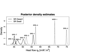
Figure 6: Estimated posterior densities of the heat flow $q_{0j}$ for boreholes from the San Rafael Desert (solid lines) and San Rafael Swell (long dashes).

Table 2: Posterior means and symmetric 90% credible intervals (CI) for the background heat flows $q_{0j}$ (mW/m²) and the mean heat flows $\nu_{D}$ and $\nu_{S}$ (mW/m²)

San Rafael Desert			San Rafael Swell
Borehole	Mean	90% CI	Borehole	Mean	90% CI
SRD-1	55.91	(55.51, 56.32)	SRS-3	51.99	(51.45, 52.54)
SRD-2	46.95	(46.02, 47.90)	SRS-4	57.25	(57.02, 57.47)
SRD-3	45.19	(44.42, 45.92)	SRS-5	74.85	(74.58, 75.11)
SRD-4	50.28	(49.54, 51.01)	WSR-1	68.13	(67.97, 68.29)
SRD-7	45.16	(44.69, 45.63)
$\nu_{D}$	55.95	(31.94, 80.39)	$\nu_{S}$	58.05	(32.93, 83.08)

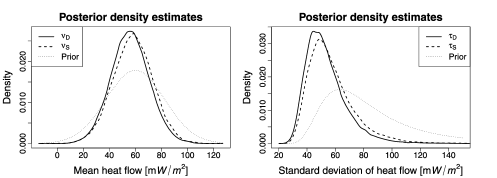
Figure 7: Estimated posterior densities of the means, $\nu_{D}$ and $\nu_{S}$ (left), and the standard deviations, $\tau_{D}$ and $\tau_{S}$ (right), of the background heat flow for both regions. The (marginal) prior distributions are the same for both regions and are presented with dotted lines.

There is considerable posterior uncertainty regarding the mean heat flows $\nu_{D}$ and $\nu_{S}$ (see Figure 7), especially when compared to the relatively precise posterior densities for the 9 individual heat flows $q_{0j}$. This is what we expect since there is substantial variation of the locations of these precise, individual densities. Another point is that the posterior means of $\nu_{D}$ and $\nu_{S}$ are surprisingly alike, and do not seem to correspond to the difference in heat flows for the two regions that is apparent in Figure 6. For example, the posterior mean of $\nu_{D}$ is higher than all the posterior means of $q_{0j}$ in the SR Desert (see Table 2). We explain this behavior in Section 4.3.2.

4.2 Comparison to single-site models

In our primary analysis we combined data from all boreholes in one hierarchical multiple-site model. The temperature histories for boreholes in the same region share the same mean and variance. Similarly, the heat flow parameters for boreholes within the same region share the same mean and variance. One rationale for doing this is that it enables us to learn about region-wide mean temperature histories and region-wide mean heat flow. Another rationale is that hierarchically linking boreholes within regions allows for sharing of information between boreholes through the shared parameters. This sharing of information across groups of data is often called borrowing strength and can often lead to better parameter estimates. However, the question here becomes how much strength, if any, is borrowed between the nine boreholes. To assess this aspect of the model, we fit single-site models described in Section 3.2 to each of the 9 boreholes.

By performing separate single-site models, we of course do not model parameters as spatially dependent. Operationally, some parameters treated as random in the combined analysis are assigned fixed values. For example, we assign values to $\bolds\mu$ and $\Gamma$ in the prior for the GST histories [see (15)], as compared to the additional stage involving $\bolds\mu_{D}$, $\bolds\mu_{S}$, $\gamma^{2}_{D}$ and $\gamma^{2}_{S}$ [see (25) and (28)] in the combined analysis. To make the results comparable, we set the prior mean and covariance matrix of the GST histories equal to their marginal prior mean and covariance implied by the multiple-site model. For boreholes in the SR Desert ($j=1,\ldots,5$), we have the following:

$$E(\mathbf{T}_{hj}) = E(E(\mathbf{T}_{hj}|\bolds\mu_{D}))=E(\bolds\mu_{D})=\bolds\mu_{0}=\mathbf{0},$$ (29)

$$\operatorname{Cov}(\mathbf{T}_{hj}) = \operatorname{Cov}(E(\mathbf{T}_{hj}|\bolds\mu_{D}))+E(\operatorname{Cov}(\mathbf{T}_{hj}|\bolds\mu_{D}))$$

$$= \operatorname{Cov}(\bolds\mu_{D})+E(\gamma^{2}_{D}I_{K})=(\sigma^{2}_{D}+\sigma^{2}_{0})I_{K}+E(\gamma^{2}_{D})I_{K}$$

$$= (0.2+0.1+0.8)I_{K}=1.1I_{K}.$$

For boreholes in the SR Swell ($j=6,\ldots,9$), we also have $E(\mathbf{T}_{hj})=E(\bolds\mu_{S})=\mathbf{0}$ and $\operatorname{Cov}(\mathbf{T}_{hj})=1.1I_{K}$. Hence, we set the following prior for $\mathbf{T}_{h}$ in the single-site models (same for every borehole):

$$\mathbf{T}_{h}\sim N(\bolds\mu,\Gamma)=N_{K}(\mathbf{0},1.1I_{K}).$$ (31)

Similarly, we set the following prior for each $q_{0}$:

$$q_{0}\sim N(0.06,0.02^{2}+0.01^{2}+0.1^{2}=0.0105).$$ (32)

Finally, we used the same priors for measurement and model error variances [see (13) and (14)] as for the multiple-site model.

We fitted the single-site models via Gibbs samplers, obtaining 10,000 MCMC samples from the posterior distribution for each borehole and deleted 2000 iterations for burn-in.

The estimated posterior means and credible sets for the GST histories from both the multiple-site and the 9 single-site models are shown in Figure 8. Focusing on the five boreholes in the SR Desert, we see two major differences. First, the GST posterior means (white squares in Figure 8) are slightly more dampened for the multiple-site model than the single-site models. In other words, we see shrinkage in the posterior means when we combine the boreholes. Second, as indicated by narrower 50% and 90% posterior credible intervals, the posterior uncertainty is substantially less for the multiple-site model than the single-site models. We conclude that by combining the boreholes in the SR Desert, the GST history parameters are borrowing strength across boreholes.

In the SR Swell the posterior results are quite similar for the multiple-site model and the single-site models. In particular, the posterior uncertainties are similar in that the 50% and 90% posterior credible intervals are only slightly wider for the single-site models than the multiple-site model. We believe that the reason for these different results for the two regions is the following: The SR Desert GST histories are comparatively similar, so the analysis amplifies combining and borrowing strength. The SR Swell results seem more diverse, suggesting borrowing strength should be comparatively weak.

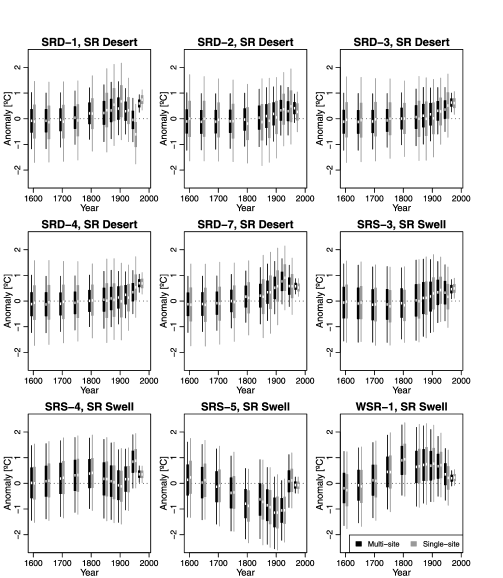
Figure 8: Comparison of posterior distributions of GST histories from the multiple-site model (black) and single-site models (grey). The white squares show the estimated posterior means and the vertical bars show the symmetric 50% (thick) and 90% (thin) posterior credible intervals.

Posterior density estimates (not shown here) for the background heat flows $q_{0j}$ and the variances $\sigma^{2}_{Y}$ and $\sigma^{2}$ were almost identical for the two analyses.

4.3 Sensitivity analyses

In our analyses we used prespecified fixed values of the temperature intercepts $T_{0j}$ and hyperparameters (i.e., fixed parameters of prior distributions). The selection of hyperparameters was discussed in Section 3.4. We next assess the sensitivity of results to some of these specifications.

4.3.1 Temperature intercept $T_{0j}$

The temperature intercepts $T_{0j}$ used here were least square estimates of the intercepts in simple linear regressions. That is, separately for each borehole, temperature data were regressed on the thermal resistance vector $\mathbf{R}_{j}$. In these steps, the regressions were based only on data at the deep parts of the borehole, specifically below 150 meters for boreholes in the SR Desert and below 200 meters for boreholes in the SR Swell. We used the usual least squares standard errors to guide our sensitivity analysis on $T_{0j}$. Specifically, we fitted the multiple-site model in two additional cases: (1) all $T_{0j}$’s were set to three standard errors below the least squares estimates and (2) all $T_{0j}$’s set to three standard errors above the least squares estimates.

Overall the results were not highly sensitive to these changes in the temperature intercepts. Estimated densities of the heat flow parameters $q_{0j}$ (not shown here) indicated that posterior for the $q_{0j}$ responded to changes in the $T_{0j}$’s as we expect a slope to change when the intercept is changed. When the $T_{0j}$ were lowered, the $q_{0j}$ were higher and vice versa. However, posterior means and standard deviations of the heat flows, $\nu_{D}$, $\nu_{S}$, $\tau_{D}$, $\tau_{S}$, and $\sigma_{Yj}$ and $\sigma_{j}$, did not vary much as we changed $T_{0j}$’s.

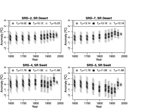
Figure 9: Comparison of posterior distributions of GST histories for 4 boreholes using different values for the temperature intercept $T_{0j}$. The white squares show the estimated posterior means and the vertical bars show the symmetric 50% (thick) and 90% (thin) posterior credible intervals. At each time point the middle bar shows the original results (same as in Figure 2) and the left and right bars show the results for lower and higher values of $T_{0j}$, respectively.

The estimated posterior means and credible sets for the GST histories for the three cases of $T_{0j}$ are shown in Figure 9. We show results for two boreholes from each region, but the effects are similar for the other boreholes. The main effect of changing the $T_{0j}$’s is that the posterior means of the GST histories are slightly shifted. The temperature anomalies are higher when $T_{0j}$ is lower and vice versa, so it seems that they are compensating the changing $T_{0j}$. Interestingly, the amount of shifting increases as we go further back in time. On the other hand, the changes in posterior means are not large when compared to the posterior uncertainty of the results. We conclude that sensitivities to the specifications of $T_{0j}$ are overshadowed by the posterior uncertainty of the results.

4.3.2 Hyperparameters $\eta_{D}$, $\eta_{S}$, $\eta_{0}$

Recalling (24), the regional prior means, $\nu_{D}$ and $\nu_{S}$, of the heat flows have prior standard deviations $(\eta^{2}_{D}+\eta^{2}_{0})^{0.5}$ and $(\eta^{2}_{S}+\eta^{2}_{0})^{0.5}$, respectively, and prior correlation $\eta^{2}_{0}/((\eta^{2}_{0}+\eta^{2}_{D})(\eta^{2}_{0}+\eta^{2}_{S}))^{0.5}$.

We report on results for four additional settings of $\eta_{0}$, $\eta_{D}$ and $\eta_{S}$ leading to the prior standard deviations and correlations given in Table 3. Note that in light of the range of heat flow estimates found in the literature (see Section 3.4), a prior standard deviation of 120 mW/m² is very large. Also, the prior correlation we selected for the original setting is very high (0.8). Note also that sensitivity settings 2 and 4 have the same correlation but different standard deviations.

Table 3: The original and four new settings of the hyperparameters $\eta^{2}_{D}$, $\eta^{2}_{S}$ and $\eta^{2}_{0}$ along with the implied prior standard deviations of $\nu_{D}$ and $\nu_{S}$ and the prior correlations between $\nu_{D}$ and $\nu_{S}$

	$\bolds{\eta^{2}_{D}}$ and $\bolds{\eta^{2}_{S}}$	$\bolds{\eta^{2}_{0}}$	Prior sd. [mW/m${}^{\bolds{2}}$]	Prior cor
Original setting	1$10^{2}$	$20^{2}$	122.36	0.80
Setting 1	1$20^{2}$	$20^{2}$	128.28	0.50
Setting 2	1$30^{2}$	$20^{2}$	136.06	0.31
Setting 3	$100^{2}$	6$0^{2}$	100.00	0.00
Setting 4	$100^{2}$	$67^{2}$	120.37	0.31

First, posterior means and credible intervals of the GST histories ($\mathbf{T}_{hj}$; not shown) were almost identical across all five cases. The same was true for the means and standard deviations of the histories ($\bolds\mu_{D}$, $\bolds\mu_{D}$, $\gamma_{D}$ and $\gamma_{S}$; not shown) Also, the posterior density estimates (not shown) for heat flow parameters $q_{j}$ were almost identical in all cases.

The posterior distributions of $\nu_{D}$ and $\nu_{S}$ displayed strong sensitivities. Figure 10 (right) shows the posterior means and credible intervals for $\nu_{D}$ and $\nu_{S}$ for all 5 settings. Not surprisingly, as the prior uncertainty increases, the posterior uncertainty increases. We note differences in the posterior means that correspond to the different prior correlations. In the original setting the posterior means of $\nu_{D}$ and $\nu_{S}$ were very close and seemed not to respond to the regional information indicated in the posteriors of the $q_{0j}$ [the vertical line segments in Figure 10 (right) are the posterior means of the $q_{0j}$; also see Table 2]. Note that as the prior correlation decreases, the posterior means of $\nu_{D}$ and $\nu_{S}$ separate and approach the averages of the heat flow posterior means in their corresponding regions. However, due to the relatively large posterior uncertainties of $\nu_{D}$ and $\nu_{S}$ in all cases, the changes we see in the posterior means are all within the 50% credible interval of the original model.

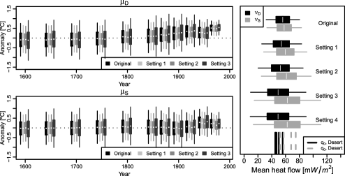
Figure 10: Left: Comparison of posterior distributions of the mean GST histories, $\bolds\mu_{D}$ and $\bolds\mu_{S}$, using different values of $\sigma^{2}_{D}$, $\sigma^{2}_{S}$ and $\sigma^{2}_{0}$ (see Table 4). The white squares show the estimated posterior means and the vertical bars show the symmetric 50% (thick) and 90% (thin) posterior credible intervals. Right: Comparison of mean heat flow $\nu_{D}$ and $\nu_{S}$ using different values of $\eta^{2}_{D}$, $\eta^{2}_{S}$ and $\eta^{2}_{0}$ (see Table 3). The white squares show the estimated posterior means and the vertical bars show the symmetric 50% (thick) and 90% (thin) posterior credible intervals. The line segments at the bottom show the posterior means of the heat flows $q_{0j}$.

Table 4: The original setting of the hyperparameters $\sigma^{2}_{D}$, $\sigma^{2}_{S}$ and $\sigma^{2}_{0}$ and the three additional settings along with the implied prior standard deviations of the elements of the vectors $\bolds\mu_{D}$ and $\bolds\mu_{S}$ and the prior correlations between $\mu_{Dk}$ and $\mu_{Sk}$ for $k=1,\ldots,K$

	$\bolds{\sigma^{2}_{D}}$ and $\bolds{\sigma^{2}_{S}}$	$\bolds{\sigma^{2}_{0}}$	Prior sd. ($\bolds{{}^{\circ}}$C)	Prior cor
Original setting	0.2	0.15	0.55	0.33
Setting 1	0.1	0.15	0.45	0.50
Setting 2	0.2	0.05	0.45	0.00
Setting 3	0.3	0.15	0.67	0.33

While these results are not surprising, it is instructive to see the workings of Bayesian updating of borrowing-strength priors. Finally, though the sample sizes at each borehole are relatively large, the operative “sample sizes” for treating $\nu_{D}$ and $\nu_{S}$ are 5 and 4 sites, respectively.

4.3.3 Hyperparameters $\sigma_{D}$, $\sigma_{S}$, $\sigma_{0}$

The hyperparameters $\sigma_{D}$, $\sigma_{S}$ and $\sigma_{0}$ determine the prior standard deviations, $(\sigma^{2}_{D}+\sigma^{2}_{0})^{0.5}$ and $(\sigma^{2}_{S}+\sigma^{2}_{0})^{0.5}$, of the elements of the prior mean GST history vectors $\bolds\mu_{D}$ and $\bolds\mu_{S}$. They also imply that the prior correlations $\operatorname{corr}(\mu_{Dk},\mu_{Sk})$, $k=1,\ldots,K$, are equal to $\sigma^{2}_{0}/((\sigma^{2}_{0}+\sigma^{2}_{D})(\sigma^{2}_{0}+\sigma^{2}_{S}))^{0.5}$. We considered three additional settings for these parameters as shown in Table 4.

Overall, the results were not sensitive to the different settings of $\sigma_{D}$, $\sigma_{S}$ and $\sigma_{0}$. The mean GST histories in each region, $\bolds\mu_{D}$ and $\bolds\mu_{S}$, were only slightly affected by the changes in the prior [see Figure 10 (left)]. The posterior credible intervals are slightly wider when the prior standard deviations are higher. The posterior means are almost identical for the four settings over the first three or four centuries. In the last century there is a slight difference between settings 1 and 2, particularly in the SR Swell. These settings have the same prior standard deviation but different prior correlations (0.5 and 0, resp.). It seems that higher prior correlation leads to posteriors that favor similarity of the elements of $\bolds\mu_{D}$ and $\bolds\mu_{S}$, but only for the more recent time points. Again, we note that these differences are very small compared to the posterior uncertainty in the results.

The results for the GST histories ($\mathbf{T}_{hj}$, not shown here) were very similar for all four settings. The only differences were that the posterior uncertainties increased slightly when the prior standard deviations of $\bolds\mu_{D}$ and $\bolds\mu_{S}$ increased. The different prior correlations did not seem to matter, settings 1 and 2 gave almost identical results. Density estimates (not shown) for other parameters were virtually identical for the different prior settings.

4.3.4 Correlated measurement and model errors

Though we expect substantial correlation among the elements of each $\mathbf{Y}_{j}$ and among the elements of each $\mathbf{T}_{rj}$, we assumed conditionally independent measurement errors and model errors in (16) and (17), respectively. The modeling notions are that the lion’s shares of these correlations are due to the structure of the true temperatures in the case of the $\mathbf{Y}_{j}$ and the structure in temperatures captured by the heat equation model in the case of the $\mathbf{T}_{rj}$ [also see Section 3.2(iii)]. Neither notion is unassailable: while the errors in (16) are due to the measurement process, they also respond to approximation errors associated with the use of the reduced temperature definition. Similarly, the errors in (17) are attributable to model approximations associated with the specifics of our use of the heat equation. However, we have virtually no prior information regarding the structure of the unmodeled physical processes; if we did know more, that knowledge could be used to improve the physical models.

Ignorance is not a valid defense for independence assumptions. Rather, those assumptions lead to obvious simplifications in the analysis and avoid difficulties associated with potential nonidentifiability issues. However, some sensitivity checks are desirable. In our setting the major concern is that incorrect assumptions of independence may lead to underestimation of uncertainties in the final results.

To assess independence assumptions, we examined model “residuals.” Some indication of structure may be developed by inspecting estimated errors defined by

$$\hat{\mathbf{e}}_{j}=\mathbf{Y}_{j}-[E(\mathbf{T}_{rj})+T_{0j}\mathbf{1}_{N_{j}}+E(q_{0j})\mathbf{R}_{j}],\qquad j=1,\ldots,9,$$ (33)

using estimated posterior expectations as indicated. A more appropriate approach is to compute

$$\mathbf{e}_{j}^{m}=\mathbf{Y}_{j}-[\mathbf{T}_{rj}^{m}+T_{0j}\mathbf{1}_{N_{j}}+q_{0j}^{m}\mathbf{R}_{j}],\qquad j=1,\ldots,9,$$ (34)

where the superscripts $m$ index MCMC iterations, though this option leads to an ensemble of residuals.

For each of the nine boreholes, we fitted time-series style ARMA models to the $\hat{\mathbf{e}}_{j}$. Though we noted some differences, AR(1) and ARMA(1,1) models provided reasonable fits. Since the forms of the covariance matrices of the AR(1) and ARMA(1,1) are quite similar, we focused on AR(1) models. We also inspected realizations of residuals as defined in (34). These residuals were similar to those based on (33), though they exhibited less structure, suggesting that basing our sensitivity checks on (33) is conservative. We replaced the covariances in (17) by the covariance matrices $\sigma_{j}^{2}\mathbf{C}(\phi)$, where $\mathbf{C}(\phi)$ is a correlation matrix with ones on the diagonal and off diagonal elements $\phi^{k}$ for every pair of depths $k$ units apart (here one unit corresponds to 5 meters). We treated $\phi$ as a known quantity and reran the MCMC analyses for two choices of $\phi$: $0.65$ and $0.85$. The final posterior results were not very different from those using the independence assumption. In Figure 11 we display comparisons of posterior distributions of GST histories for two boreholes for each of the Desert and Swell regions as well as the corresponding region mean processes. The boreholes were selected to indicate the range of differences, that is, one borehole showing the least differences and another one showing the most differences. We did observe nonnegligible increases in the spreads of the posteriors for the heat flow parameters $q_{0j}$, though there were virtually no changes in their means.

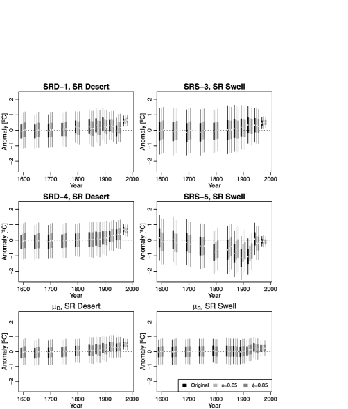
Figure 11: Comparison of posterior distributions of GST histories for 4 boreholes and the mean histories $\bolds\mu_{D}$ and $\bolds\mu_{S}$ using model error covariance matrices $\sigma_{j}^{2}\mathbf{C}(\phi)$ with different values of $\phi$. The white squares show the estimated posterior means and the vertical bars show the symmetric 50% (thick) and 90% (thin) posterior credible intervals. At each time point the first (darkest) bar shows the original results ($\phi=0$; same as in Figure 2) and the next two bars show the results for $\phi=0.65$ and $\phi=0.85$.

We repeated this process by replacing the model error covariances in (16) by matrices $\sigma_{Y_{j}}^{2}\mathbf{C}(\phi)$ for the same two values of $\phi$. The same behaviors were observed; indeed, the differences were smaller that those above. Hence, though some structure in the errors are unmodeled in this article, the effects of this appear to be very minor in the posterior inferences regarding GST histories.

5 Discussion

We developed Bayesian hierarchical models featuring two key aspects: (1) the use of a physics based model having uncertain parameters and subject to model error, and (2) the illustration of borrowing strength based on priors on selected parameters to combine data sets. In the first development we relied on a common framework to define reduced temperatures $\mathbf{T}_{r}$ to justify use of the heat equation as the main physical model. However, we added the treatment of background surface heat flows $q_{0}$ as unknown parameters and the inclusion of model errors implying a random heat equation model. The hierarchical modeling approach also allows us to separate explicitly measurement errors from model errors. These steps support the claim that our models account for important uncertainties.

In our prior distributions we modeled the surface history processes and background heat flows as arising from region-specific (SR Desert or SR Swell) models, which in turn have parameters generated from a San Rafael basin-wide prior model. These formulations led to posterior results that display very notable and appropriate behaviors. As discussed in Section 4.2, the inferences for model parameters and histories in the SR Desert region indicated borrowing strength in concert with the similarities of behaviors at individual boreholes. By comparison, we noted very little borrowing of strength in the SR Swell region where the individual results were comparatively dissimilar. We find this result quite satisfactory and illustrative, but should note that the priors used were extremely simple. They were chosen because we had little prior information and too little data (i.e., four and five boreholes in the two regions) on which to update more intense priors. When feasible, we recommend consideration of more intense spatial process priors for parameters. See Cressie (1993) and Banerjee, Carlin and Gelfand (2004) for discussion of sophisticated spatial models.

As is appropriate in most Bayesian analyses, we devoted substantial attention to sensitivity analyses. The results are discussed in Section 4 and not reviewed here. However, note that we did not present analyses regarding the specification of the thermal conductivities ($k$) used in defining the vectors of thermal resistance vectors $\mathbf{R}$. Very cursory inspections suggest to us that the approach may be very sensitive to these quantities. We will pursue this aspect in an alternative modeling approach to be reported on elsewhere.

We note that the results lead to the suggestion that borehole data are useful in inferring surface temperatures for times from the recent past to about 200 years in the past. For times deeper in the past, the borehole data appear to be comparatively less informative. We base this suggestion on the behavior of the posterior distributions of the site-wise histories as well as the SR Desert and Swell mean histories. These distributions seem to asymptote to region-specific distributions. For all times before 1800 and all five boreholes in the SR Desert, the posterior standard deviations of historical temperatures vary between $0.61$ and $0.68$ (only 5 of the 35 values are less than $0.65$); these values are 2 or 3 times larger than the standard deviations for temperatures in the Desert in 1980. In the SR Swell, all 28 of the corresponding standard deviations are between $0.87$ and $0.95$, and are roughly 4 times the standard deviations for temperatures in the Swell in 1980. Regarding this issue, North et al. [(2006), page 80] write the following:

The time resolution and length of borehole-based surface temperature reconstructions are severely limited by the physics of the heat transfer process…. A surface temperature signal is irrecoverably smeared as it is transferred to depth. The time resolution of the reconstruction thus decreases backward in time. For rock and permafrost boreholes, this resolution is a few decades at the start of the 20th century and a few centuries at 1500.

For related discussion see Beltrami and Mareschal (1995) and Hopcroft, Gallagher and Pain (2007). Our addition to these claims is that the posterior standard deviations based on models that include model error and other uncertainties are roughly constant by necessity for times beyond 200 years in the past. Of course, this is based on limited data from a limited region and need not apply in greater generality.

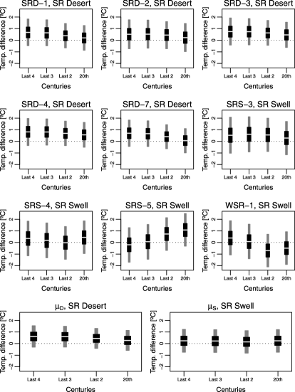
Figure 12: Posterior means and credible sets of surface temperature changes over the four periods 1600, 1700, 1800 and 1900 to the latest year in our data sets (1980) for each of the nine boreholes and for the SR Desert and SR Swell means. The vertical bars show the symmetric 50% (thicker) and 90% (thinner) posterior credible intervals and the grey horizontal lines show the posterior means.

To characterize our results in regard to climate change, we provide inferences on the changes in surface temperatures over the four periods 1600, 1700, 1800 and 1900 to the latest year in our data sets (1980) for each of the nine boreholes and for the SR Desert and SR Swell means (see Figure 12). We note that the point estimates of these changes are typically positive (i.e., increased temperature) for the individual boreholes and are all positive for the basin-wide means. However, all $90\%$ credible intervals cover $0^{\circ}$C, though many of the $50\%$ credible intervals lie above $0^{\circ}$C. Based on the common trend in these results, we believe that the suggestion of warming is supported. While the strength of this support is not strong, we note that our sample sizes are very small. Further, since our data ends in 1980, we cannot find the more recent warming reflected in other data. Finally, we caution that traditional quantification associated with so-called statistical significance (i.e., $90\%$ or $95\%$ intervals not covering 0) are of little relevance in regard to decision making in the context of climate change.

Appendix A List of parameters

Unknown parameters:

Borehole specific parameters ($j=1,\ldots,9$):

• [$\sigma^{2}_{Yj}$:]

• Temperature histories, vectors of dimension $K$.

• True reduced temperatures, vectors of dimension $N_{j}$.

• Heat flows, scalars.

• Measurement error variances.

• Model error variances.

Region specific parameters:

• [$\bolds\mu_{D}$, $\bolds\mu_{S}$:]

• Mean temperature histories for SR Desert (D) and SR Swell (S), vectors of dimension $K$.

• Variances of temperature histories for SR Desert (D) and SR Swell (S).

• Mean heat flow for SR Desert (D) and Swell (S), scalars.

• Variances of heat flow for SR Desert (D) and Swell (S).

Hyperparameters–constants:

• [$\sigma^{2}_{0}$, $\sigma^{2}_{D}$, $\sigma^{2}_{S}$:]

• Prior mean of $\bolds\mu_{D}$ and $\bolds\mu_{S}$.

• Define the prior covariance structure of $\bolds\mu_{D}$ and $\bolds\mu_{S}$.

• Prior mean of $\nu_{D}$ and $\nu_{S}$.

• Define the prior covariance structure of $\nu_{D}$ and $\nu_{S}$.

• Define the Inverse Gamma prior for $\sigma^{2}_{Yj}$.

• Define the Inverse Gamma prior for $\sigma^{2}_{j}$.

• Define the Inverse Gamma prior for $\gamma^{2}_{D}$ and $\gamma^{2}_{S}$.

• Define the Inverse Gamma prior for $\tau^{2}_{D}$ and $\tau^{2}_{S}$.

Appendix B Gibbs sampler

A Gibbs sampler is a method that obtains approximate samples from the posterior distribution. It avoids the big dimensionality of the model by simulating only parts of the parameters at a time, using the so-called full conditional distributions. The notation $[X|\cdot]$ reads “the full conditional distribution of $X$ given all other parameters and the data.” Also, $\|\mathbf{x}\|=\mathbf{x}^{\prime}\mathbf{x}$, for a vector $\mathbf{x}$.

GST history vectors $\mathbf{T}_{hj}$ and reduced temperature vectors $\mathbf{T}_{rj}$

To make the Gibbs sampler more efficient, we sample the joint full conditional distribution $\mathbf{T}_{hj},\mathbf{T}_{rj}|\cdot$ for each borehole $j$. Note that the joint (prior) distribution of $\mathbf{T}_{hj}$ and $\mathbf{T}_{rj}$ for boreholes in the SR desert ($j=1,\ldots,5$) is

$$\pmatrix{\displaystyle\mathbf{T}_{rj}\cr\displaystyle\mathbf{T}_{hj}}\sim N\left(\pmatrix{\displaystyle A_{j}\bolds\mu_{D}\cr\displaystyle\bolds\mu_{D}},\pmatrix{\displaystyle\widetilde{\Sigma}_{j}&\gamma^{2}_{D}A_{j}\cr\displaystyle\gamma^{2}_{D}A_{j}^{\prime}&\gamma^{2}_{D}I_{K}}\right),$$ (35)

where

$$\widetilde{\Sigma}_{j}=\sigma_{j}^{2}I_{N_{j}}+\gamma^{2}_{D}A_{j}A_{j}^{\prime}.$$ (36)

The joint full conditional distribution of $\mathbf{T}_{rj}$ and $\mathbf{T}_{hj}$ given $\mathbf{Y}_{j}$ and all other parameters, which we denote by $\Theta$, can be written as follows:

$$[\mathbf{T}_{rj},\mathbf{T}_{hj}|\mathbf{Y}_{j},\Theta] = \frac{[\mathbf{Y}_{j}|\mathbf{T}_{rj},\Theta][\mathbf{T}_{rj}|\Theta]}{[\mathbf{Y}_{j}|\Theta]}[\mathbf{T}_{hj}|\mathbf{T}_{rj},\Theta]$$

$$= [\mathbf{T}_{rj}|\mathbf{Y}_{j},\Theta][\mathbf{T}_{hj}|\mathbf{T}_{rj},\Theta].$$

Therefore, to sample $\mathbf{T}_{hj},\mathbf{T}_{rj}|\cdot$, we first sample the marginal distribution $[\mathbf{T}_{rj}|\mathbf{Y}_{j},\Theta]$ and then the conditional distribution $[\mathbf{T}_{hj}|\mathbf{T}_{rj},\Theta]$. First note that $[\mathbf{T}_{rj}|\mathbf{Y}_{j},\Theta]$ is proportional to $[\mathbf{Y}_{j}|\mathbf{T}_{rj},\Theta][\mathbf{T}_{rj}|\Theta]$ where $[\mathbf{T}_{rj}|\Theta]$ is the marginal distribution of the joint prior (35). Therefore, for boreholes in the SR Desert ($j=1,\ldots,5$), we have $[\mathbf{T}_{rj}|\mathbf{Y}_{j},\Theta]=N(Dd,D)$, where

$$D=\biggl{(}\frac{1}{\sigma_{Yj}^{2}}I_{N_{j}}+\widetilde{\Sigma}_{j}^{-1}\biggr{)}^{-1}$$ (38)

and

$$d=\bigl{(}\mathbf{Y}_{j}-(T_{0j}\mathbf{1}_{N_{j}}+q_{j}\mathbf{R}_{j})\bigr{)}/\sigma_{Yj}^{2}+\widetilde{\Sigma}_{j}^{-1}A_{j}\bolds\mu_{D}.$$ (39)

Second, note that $[\mathbf{T}_{hj}|\mathbf{T}_{rj},\Theta]$ is the conditional prior distribution

$$N\bigl{(}\bolds\mu_{D}+\gamma^{2}_{D}A_{j}^{\prime}\widetilde{\Sigma}_{j}^{-1}(\mathbf{T}_{rj}-A_{j}\bolds\mu_{D}),\gamma^{2}_{D}I_{K}-\gamma^{4}_{D}A_{j}^{\prime}\widetilde{\Sigma}_{j}^{-1}A_{j}\bigr{)}.$$ (40)

For boreholes in the SR Swell ($j=6,\ldots,9$), we replace $\bolds\mu_{D}$ in (39) and (40) with $\bolds\mu_{S}$ and $\gamma^{2}_{D}$ in (40) and (36) with $\gamma^{2}_{S}$.

Measurement and model error variances, $\sigma^{2}_{Yj}$ and $\sigma^{2}_{j}$

$$\sigma^{2}_{Yj}|\cdot \sim IG\biggl{(}\frac{N_{j}}{2}+a_{Y},b_{Y}+\frac{1}{2}\|\mathbf{Y}_{j}-(\mathbf{T}_{rj}+T_{0j}\mathbf{1}_{N_{j}}+q_{j}\mathbf{R}_{j})\|\biggr{)},$$ (41)

$$\sigma_{j}^{2}|\cdot \sim IG\biggl{(}\frac{N_{j}}{2}+a,b+\frac{1}{2}\|\mathbf{T}_{rj}-A_{j}\mathbf{T}_{hj}\|\biggr{)},\qquad j=1,\ldots,9.$$ (42)

Mean and variances of the GST history, $\bolds\mu_{D}$, $\bolds\mu_{S}$, $\gamma^{2}_{D}$ and $\gamma^{2}_{D}$

We sample the joint full conditional distribution of $\bolds\mu_{D}$ and $\bolds\mu_{S}$. We have $\bolds\mu_{D},\bolds\mu_{S}|\cdot\sim N(Dd,D)$ with

$$D=\frac{1}{w}\pmatrix{\displaystyle\biggl{(}\frac{4}{\gamma^{2}_{S}}+\frac{\sigma^{2}_{D}+\sigma^{2}_{0}}{v}\biggr{)}I_{K}&\displaystyle\frac{\sigma^{2}_{0}}{v}I_{K}\cr\displaystyle\frac{\sigma^{2}_{0}}{v}I_{K}&\displaystyle\biggl{(}\frac{5}{\gamma^{2}_{D}}+\frac{\sigma^{2}_{S}+\sigma^{2}_{0}}{v}\biggr{)}I_{K}}$$ (43)

and

$$d=\pmatrix{\displaystyle\frac{1}{\gamma^{2}_{D}}\sum_{j=1}^{5}\mathbf{T}_{hj}\cr\displaystyle\frac{1}{\gamma^{2}_{S}}\sum_{j=6}^{9}\mathbf{T}_{hj}}+\frac{1}{v}\pmatrix{\displaystyle\sigma^{2}_{S}\bolds\mu_{0}\cr\displaystyle\sigma^{2}_{D}\bolds\mu_{0}},$$ (44)

where $w=(\frac{5}{\gamma^{2}_{D}}+\frac{\sigma^{2}_{S}+\sigma^{2}_{0}}{v})(\frac{4}{\gamma^{2}_{S}}+\frac{\sigma^{2}_{D}+\sigma^{2}_{0}}{v})-\frac{\sigma^{4}_{0}}{v^{2}}$ and $v=(\sigma^{2}_{D}+\sigma^{2}_{0})(\sigma^{2}_{S}+\sigma^{2}_{0})-\sigma^{4}_{0}$.

The variances of the GST histories are sampled separately for each region,

$$\gamma_{D}^{2}|\cdot\sim IG\Biggl{(}5K/2+a_{\gamma},b_{\gamma}+\frac{1}{2}\sum_{j=1}^{5}\|\mathbf{T}_{hj}-\bolds\mu_{D}\|\Biggr{)}$$ (45)

and

$$\gamma_{S}^{2}|\cdot\sim IG\Biggl{(}4K/2+a_{\gamma},b_{\gamma}+\frac{1}{2}\sum_{j=6}^{9}\|\mathbf{T}_{hj}-\bolds\mu_{S}\|\Biggr{)}.$$ (46)

Heat flow parameters $q_{0j}$, $\nu_{D}$, $\nu_{S}$, $\tau^{2}_{D}$, $\tau^{2}_{S}$

For boreholes in the SR Desert ($j=1,\ldots,5$), we have

$$q_{j}|\cdot\sim N\biggl{(}\frac{\tau_{D}^{2}\mathbf{R}_{j}^{\prime}(\mathbf{Y}_{j}-\mathbf{T}_{rj}-T_{0j}\mathbf{1}_{N_{j}})+\sigma_{Yj}^{2}\nu_{D}}{\tau_{D}^{2}\mathbf{R}_{j}^{\prime}\mathbf{R}_{j}+\sigma_{Yj}^{2}},\frac{\tau_{D}^{2}\sigma_{Yj}^{2}}{\tau_{D}^{2}\mathbf{R}_{j}^{\prime}\mathbf{R}_{j}+\sigma_{Yj}^{2}}\biggr{)}.$$ (47)

For boreholes in the SR Swell ($j=6,\ldots,9$), we replace $\bolds\mu_{D}$ and $\tau^{2}_{D}$ in (47) by $\bolds\mu_{S}$ and $\tau^{2}_{S}$.

The mean heat flow parameters $\nu_{D}$ and $\nu_{S}$ are sampled from a joint distribution $\nu_{D},\nu_{S}|\cdot\sim N(Dd,D)$ with

$$D=\frac{1}{w}\pmatrix{\displaystyle\frac{4}{\tau^{2}_{S}}+\frac{\eta^{2}+\eta^{2}_{0}}{v}&\displaystyle\frac{\eta^{2}_{0}}{v}\cr\displaystyle\frac{\eta^{2}_{0}}{v}&\displaystyle\frac{5}{\tau^{2}_{D}}+\frac{\eta^{2}+\eta^{2}_{0}}{v}}$$ (48)

and

$$d=\pmatrix{\displaystyle\frac{1}{\tau^{2}_{D}}\sum_{j=1}^{5}q_{j}\cr\displaystyle\frac{1}{\tau^{2}_{S}}\sum_{j=6}^{9}q_{j}}+\frac{1}{v}\pmatrix{\displaystyle\eta^{2}\nu_{0}\cr\displaystyle\eta^{2}\nu_{0}},$$ (49)

where $w=(\frac{5}{\tau^{2}_{D}}+\frac{\eta^{2}+\eta^{2}_{0}}{v})(\frac{4}{\tau^{2}_{S}}+\frac{\eta^{2}+\eta^{2}_{0}}{v})-\frac{\eta^{4}_{0}}{v^{2}}$ and $v=(\eta^{2}+\eta^{2}_{0})^{2}-\eta^{4}_{0}$.

Finally, the variances of the heat flow are sampled separately for each region,

$$\tau_{D}^{2}|\cdot\sim IG\Biggl{(}5/2+a_{\tau},b_{\tau}+\frac{1}{2}\sum_{j=1}^{5}(q_{j}-\nu_{D})^{2}\Biggr{)}$$ (50)

and

$$\tau_{S}^{2}|\cdot\sim IG\Biggl{(}4/2+a_{\tau},b_{\tau}+\frac{1}{2}\sum_{j=6}^{9}(q_{j}-\nu_{S})^{2}\Biggr{)}.$$ (51)

References

- Banerjee, Carlin and Gelfand (2004) {bbook}[author] \bauthor\bsnmBanerjee, \bfnmSudipto\binitsS., \bauthor\bsnmCarlin, \bfnmBradley P.\binitsB. P. and \bauthor\bsnmGelfand, \bfnmAlan E.\binitsA. E. (\byear2004). \btitleHierarchical Modeling and Analysis for Spatial Data. \bpublisherChapman & Hall/CRC Press, \baddressBoca Raton, FL. \endbibitem
- Beltrami and Mareschal (1991) {barticle}[author] \bauthor\bsnmBeltrami, \bfnmHugo\binitsH. and \bauthor\bsnmMareschal, \bfnmJean-Claude\binitsJ.-C. (\byear1991). \btitleRecent warming in eastern Canada inferred from geothermal measurements. \bjournalGeophysical Research Letters \bvolume18 \bpages605–608. \endbibitem
- Beltrami and Mareschal (1995) {barticle}[author] \bauthor\bsnmBeltrami, \bfnmHugo\binitsH. and \bauthor\bsnmMareschal, \bfnmJean-Claude\binitsJ.-C. (\byear1995). \btitleResolution of ground temperature histories inverted from borehole temperature data. \bjournalGlobal and Planetary Change \bvolume11 \bpages57–70. \endbibitem
- Berger (1985) {bbook}[author] \bauthor\bsnmBerger, \bfnmJames O.\binitsJ. O. (\byear1985). \btitleStatistical Decision Theory and Bayesian Analysis, \bedition2nd ed. \bpublisherSpringer, \baddressNew York. \MR0804611 \endbibitem
- Berliner (2003) {barticle}[author] \bauthor\bsnmBerliner, \bfnmL. Mark\binitsL. M. (\byear2003). \btitlePhysical-statistical modeling in geophysics. \bjournalJournal of Geophysical Research \bvolume108 \bpages1–10. DOI: 10.1029/2002JD002865. \endbibitem
- Berliner et al. (2008) {barticle}[author] \bauthor\bsnmBerliner, \bfnmL. M.\binitsL. M., \bauthor\bsnmJezek, \bfnmK.\binitsK., \bauthor\bsnmCressie, \bfnmN.\binitsN., \bauthor\bsnmKim, \bfnmY.\binitsY., \bauthor\bsnmLam, \bfnmC. Q.\binitsC. Q. and \bauthor\bparticlevan der \bsnmVeen, \bfnmC. J.\binitsC. J. (\byear2008). \btitleModeling dynamic controls on ice streams: A Bayesian statistical approach. \bjournalJournal of Glaciology \bvolume54 \bpages705–714. \endbibitem
- Bodell and Chapman (1982) {barticle}[author] \bauthor\bsnmBodell, \bfnmJohn Michael\binitsJ. M. and \bauthor\bsnmChapman, \bfnmDavid S.\binitsD. S. (\byear1982). \btitleHeat flow in the north-central Colorado Plateau. \bjournalJournal of Geophysical Research \bvolume87 \bpages2869–2884. \endbibitem
- Carlslaw and Jaeger (1959) {bbook}[author] \bauthor\bsnmCarlslaw, \bfnmH. S.\binitsH. S. and \bauthor\bsnmJaeger, \bfnmJ. C.\binitsJ. C. (\byear1959). \btitleConduction of Heat in Solids. \bpublisherOxford Univ. Press, \baddressNew York. \MR0106686 \endbibitem
- Cressie (1993) {bbook}[author] \bauthor\bsnmCressie, \bfnmN. A. C.\binitsN. A. C. (\byear1993). \btitleStatistics for Spatial Data. \bpublisherWiley, \baddressNew York. \MR1239641 \endbibitem
- Dorofeeva, Shen and Shapova (2002) {barticle}[author] \bauthor\bsnmDorofeeva, \bfnmR. P.\binitsR. P., \bauthor\bsnmShen, \bfnmPo Yu\binitsP. Y. and \bauthor\bsnmShapova, \bfnmM. V.\binitsM. V. (\byear2002). \btitleGround surface temperature histories inferred from deep borehole temperature-depth data in Eastern Siberia. \bjournalEarth and Planetary Science Letters \bvolume203 \bpages1059–1071. \endbibitem
- Harris and Chapman (1995) {barticle}[author] \bauthor\bsnmHarris, \bfnmRobert N.\binitsR. N. and \bauthor\bsnmChapman, \bfnmDavid S.\binitsD. S. (\byear1995). \btitleClimate change on the Colorado Plateau of eastern Utah inferred from borehole temperatures. \bjournalJournal of Geophysical Research \bvolume100 \bpages6367–6381. \endbibitem
- Harris and Chapman (1998) {barticle}[author] \bauthor\bsnmHarris, \bfnmRobert N.\binitsR. N. and \bauthor\bsnmChapman, \bfnmDavid S.\binitsD. S. (\byear1998). \btitleGeothermics and climate change 1. Analysis of borehole temperature with emphasis on resolving power. \bjournalJournal of Geophysical Research \bvolume103 \bpages7363–7370. \endbibitem
- Haslett et al. (2006) {barticle}[author] \bauthor\bsnmHaslett, \bfnmJ.\binitsJ., \bauthor\bsnmWhiley, \bfnmM.\binitsM., \bauthor\bsnmBhattacharya, \bfnmS.\binitsS., \bauthor\bsnmSalter-Townshend, \bfnmM.\binitsM., \bauthor\bsnmWilson, \bfnmS. P.\binitsS. P., \bauthor\bsnmAllen, \bfnmJ. R. M.\binitsJ. R. M., \bauthor\bsnmHuntley, \bfnmB.\binitsB. and \bauthor\bsnmMitchell, \bfnmF. J. G.\binitsF. J. G. (\byear2006). \btitleBayesian palaeoclimate reconstruction. \bjournalJ. Roy. Statist. Soc. Ser. A \bvolume169 \bpages395–438. \MR2236914 \endbibitem
- Hopcroft, Gallagher and Pain (2007) {barticle}[author] \bauthor\bsnmHopcroft, \bfnmPeter O.\binitsP. O., \bauthor\bsnmGallagher, \bfnmKerry\binitsK. and \bauthor\bsnmPain, \bfnmChris C.\binitsC. C. (\byear2007). \btitleInference of past climate from borehole temperature data using Baysian Reversible Jump Markov chain Monte Carlo. \bjournalGeophysical Journal International \bvolume171 \bpages1430–1439. \endbibitem
- Jansen et al. (2007) {binproceedings}[author] \bauthor\bsnmJansen, \bfnmE.\binitsE. \betalet al. (\byear2007). \btitlePaleoclimate. In \bbooktitleClimate Change 2007: The Physical Science Basis. Contributions of Working Group I to the Fourth Assessment Report of the Intergovernmental Panel on Climate Change (\beditorS. Solomon et al., eds.) \bpages433–497. \bpublisherCambridge Univ. Press, \baddressCambridge. \endbibitem
- Li, Nychka and Ammann (2007) {barticle}[author] \bauthor\bsnmLi, \bfnmBo\binitsB., \bauthor\bsnmNychka, \bfnmDouglas W.\binitsD. W. and \bauthor\bsnmAmmann, \bfnmCaspar M.\binitsC. M. (\byear2007). \btitleThe ‘hockey’ stick and the 1990s: A statistical perspective on reconstructing hemispheric temperatures. \bjournalTellus \bvolume59A \bpages591–598. \endbibitem
- Li, Nychka and Ammann (2010) {barticle}[author] \bauthor\bsnmLi, \bfnmBo\binitsB., \bauthor\bsnmNychka, \bfnmDouglas W.\binitsD. W. and \bauthor\bsnmAmmann, \bfnmCaspar M.\binitsC. M. (\byear2010). \btitleThe value of multi-proxy reconstruction of past climate. \bjournalJ. Amer. Statist. Assoc. \bvolume105 \bpages883–895. \endbibitem
- Mareschal and Beltrami (1992) {barticle}[author] \bauthor\bsnmMareschal, \bfnmJean-Claude\binitsJ.-C. and \bauthor\bsnmBeltrami, \bfnmHugo\binitsH. (\byear1992). \btitleEvidence for recent warming from perturbed geothermal gradients: Examples from eastern Canada. \bjournalClimate Dynamics \bvolume6 \bpages135–143. \endbibitem
- North et al. (2006) {bbook}[author] \bauthor\bsnmNorth, \bfnmG. R.\binitsG. R. \betalet al. (\byear2006). \btitleSurface Temperature Reconstructions for the Last 2000 Years. \bpublisherNational Academy Press, \baddressWashington, DC. \endbibitem
- Pollack, Huang and Shen (1998) {barticle}[author] \bauthor\bsnmPollack, \bfnmHenry N.\binitsH. N., \bauthor\bsnmHuang, \bfnmShaopeng\binitsS. and \bauthor\bsnmShen, \bfnmPo Yu\binitsP. Y. (\byear1998). \btitleClimate change record in subsurface temperatures: A global perspective. \bjournalScience \bvolume282 \bpages279–281. \endbibitem
- Shen and Beck (1991) {barticle}[author] \bauthor\bsnmShen, \bfnmPo Yu\binitsP. Y. and \bauthor\bsnmBeck, \bfnmA. E.\binitsA. E. (\byear1991). \btitleLeast squares inversion of borehole temperature measurements in functional space. \bjournalJournal of Geophysical Research \bvolume96 \bpages19965–19979. \endbibitem
- Shen and Beck (1992) {barticle}[author] \bauthor\bsnmShen, \bfnmPo Yu\binitsP. Y. and \bauthor\bsnmBeck, \bfnmA. E.\binitsA. E. (\byear1992). \btitlePaleoclimate change and heat flow density inferred from temperature data in the Superior Province of the Canadian Shield. \bjournalPalaeogeography, Palaeoclimatology, Palaeoecology \bvolume98 \bpages143–165. \endbibitem
- Shen et al. (1992) {barticle}[author] \bauthor\bsnmShen, \bfnmPo Yu\binitsP. Y., \bauthor\bsnmWang, \bfnmK.\binitsK., \bauthor\bsnmBeltrami, \bfnmHugo\binitsH. and \bauthor\bsnmMareschal, \bfnmJ. C.\binitsJ. C. (\byear1992). \btitleA comparative study of inverse methods for estimating climatic history from borehole temperature data. \bjournalPalaeogeography, Palaeoclimatology, Palaeoecology \bvolume98 \bpages113–127. \endbibitem
- Smith, Berliner and Guttorp (2010) {barticle}[author] \bauthor\bsnmSmith, \bfnmR. L.\binitsR. L., \bauthor\bsnmBerliner, \bfnmL. M.\binitsL. M. and \bauthor\bsnmGuttorp, \bfnmP.\binitsP. (\byear2010). \btitleStatisticians comment on status of climate change science. \bjournalAmstat News \bvolume393 \bpages13–17. \endbibitem
- Vasseur et al. (1983) {barticle}[author] \bauthor\bsnmVasseur, \bfnmG.\binitsG., \bauthor\bsnmBernard, \bfnmPh.\binitsP., \bauthor\bparticlevan de \bsnmMeulerbrouck, \bfnmJ.\binitsJ., \bauthor\bsnmKast, \bfnmY.\binitsY. and \bauthor\bsnmJolivet, \bfnmJ.\binitsJ. (\byear1983). \btitleHolocene Paleotemperatures deduced from geothermal measurements. \bjournalPalaeogeography, Palaeoclimatology, Palaeoecology \bvolume43 \bpages237–259. \endbibitem
- Wegman, Scott and Said (2006) {bbook}[author] \bauthor\bsnmWegman, \bfnmE. J.\binitsE. J., \bauthor\bsnmScott, \bfnmD. W.\binitsD. W. and \bauthor\bsnmSaid, \bfnmY. H.\binitsY. H. (\byear2006). \btitleAd Hoc Committee Report on the ‘Hockey Stick’ Global Climate Reconstruction. Report to the Committee on Energy and Commerce. \bpublisherUnited States House of Representatives, \baddressWashington, DC. \endbibitem
- Wikle et al. (2001) {barticle}[author] \bauthor\bsnmWikle, \bfnmChristopher K.\binitsC. K., \bauthor\bsnmMilliff, \bfnmRalph F.\binitsR. F., \bauthor\bsnmNychka, \bfnmDoug\binitsD. and \bauthor\bsnmBerliner, \bfnmL. Mark\binitsL. M. (\byear2001). \btitleSpatiotemporal hierarchical Bayesian modeling: Tropical ocean surface winds. \bjournalJ. Amer. Statist. Assoc. \bvolume96 \bpages382–397. \MR1939342 \endbibitem