Abstract
A branching process of particles moving at finite velocity over the geodesic lines of the hyperbolic space (Poincaré half-plane and Poincaré disk) is examined. Each particle can split into two particles only once at Poisson paced times and deviates orthogonally when splitted. At time t 𝑡 t N ( t ) 𝑁 𝑡 N(t) N ( t ) + 1 𝑁 𝑡 1 N(t)+1 t 𝑡 t c 𝑐 c λ 𝜆 \lambda
Keywords: Branching processes, difference-differential equations, hyperbolic Brownian motion, hyperbolic trigonometry, Laplace transforms, non-Euclidean geometry, random motions.
1 Introduction
Random motions in hyperbolic spaces have been studied since the Fifties and much emphasis has been placed on the so-called hyperbolic Brownian motion on the Poincaré half-plane (see, e.g., Gertsenshtein and Vasiliev [3 ] , Getoor [4 ] , Gruet [6 ] , and Lao and Orsingher [9 ] ).
Hyperbolic Brownian motion has been revitalized by mathematical finance since some exotic financial products (Asian options) have a strict connection with the stochastic representation of the hyperbolic Brownian motion (Yor [14 ] ).
Branching hyperbolic Brownian motion has been analyzed by Lalley and Sellke [10 ] who investigated the connection between the birth rate and the underlying dynamics in supercritical and subcritical cases. Also Kelbert and Suhov [7 ] , [8 ] have studied the asymptotic behavior of the hyperbolic branching Brownian motion, developing the ideas in [3 ] and [10 ] .
The space on which the above considered hyperbolic Brownian motions develop is the Poincaré half-plane (and its higher-dimensional equivalents, see Gruet [5 ] ) or the Klein model (see [7 ] and [8 ] ).
The half-plane Poincaré model is a fine tool to describe the light propagation in a non-homogeneous medium where, on the basis of Fermat’s principle, the angle α ( y ) 𝛼 𝑦 \alpha(y) y 𝑦 y [ sin α ( y ) ] / [ c y ] = 1 / k delimited-[] 𝛼 𝑦 delimited-[] 𝑐 𝑦 1 𝑘 [{\sin\alpha(y)}]/[{cy}]={1}/{k}
Random motions with finite velocity have been considered in Orsingher and De Gregorio [12 ] (on H 2 + superscript subscript 𝐻 2 H_{2}^{+}
Several models of random motions in H 2 + superscript subscript 𝐻 2 H_{2}^{+} [1 ] , where the components of the motion have been assumed dependent and the particle moves on mutually orthogonal geodesic lines.
Here we study a random motion of a cloud of particles moving at finite velocity on geodesic lines of the hyperbolic space H 2 + superscript subscript 𝐻 2 H_{2}^{+} O 𝑂 O H 2 + superscript subscript 𝐻 2 H_{2}^{+} λ 𝜆 \lambda c 𝑐 c 1 / 2 1 2 1/2 1 / 2 2 1 superscript 2 2 1/2^{2} O 𝑂 O 1 k 𝑘 k 1 / 2 k 1 superscript 2 𝑘 1/2^{k} 1 / 2 k + 1 1 superscript 2 𝑘 1 1/2^{k+1}
If up to time t 𝑡 t N ( t ) 𝑁 𝑡 N(t) N ( t ) + 1 𝑁 𝑡 1 N(t)+1 c 𝑐 c
In the above branching process each particle can reproduce only once and the particle splitting at time T k subscript 𝑇 𝑘 T_{k} k 𝑘 k 1 / 2 k 1 superscript 2 𝑘 1/2^{k} ( T k , t ) subscript 𝑇 𝑘 𝑡 (T_{k},t)
Our main result concerns the dynamics of the center of mass c m 𝑐 𝑚 cm O 𝑂 O η c m ( t ) subscript 𝜂 𝑐 𝑚 𝑡 \eta_{cm}(t) c m 𝑐 𝑚 cm t > 0 𝑡 0 t>0
E { cosh η c m ( t ) } 𝐸 subscript 𝜂 𝑐 𝑚 𝑡 \displaystyle E\{\cosh\eta_{cm}(t)\} = \displaystyle= 2 3 c 2 e − 3 2 2 λ t λ 2 + 2 4 c 2 { e − t 2 2 λ 2 + 2 4 c 2 3 λ 2 + 2 4 c 2 + 5 λ + e t 2 2 λ 2 + 2 4 c 2 3 λ 2 + 2 4 c 2 − 5 λ } superscript 2 3 superscript 𝑐 2 superscript 𝑒 3 superscript 2 2 𝜆 𝑡 superscript 𝜆 2 superscript 2 4 superscript 𝑐 2 superscript 𝑒 𝑡 superscript 2 2 superscript 𝜆 2 superscript 2 4 superscript 𝑐 2 3 superscript 𝜆 2 superscript 2 4 superscript 𝑐 2 5 𝜆 superscript 𝑒 𝑡 superscript 2 2 superscript 𝜆 2 superscript 2 4 superscript 𝑐 2 3 superscript 𝜆 2 superscript 2 4 superscript 𝑐 2 5 𝜆 \displaystyle\frac{2^{3}c^{2}e^{-\frac{3}{2^{2}}\lambda t}}{\sqrt{\lambda^{2}+2^{4}c^{2}}}\left\{\frac{e^{-\frac{t}{2^{2}}\sqrt{\lambda^{2}+2^{4}c^{2}}}}{3\sqrt{\lambda^{2}+2^{4}c^{2}}+5\lambda}+\frac{e^{\frac{t}{2^{2}}\sqrt{\lambda^{2}+2^{4}c^{2}}}}{3\sqrt{\lambda^{2}+2^{4}c^{2}}-5\lambda}\right\}
+ λ + 2 c 2 ( λ + 3 c ) e c t + λ − 2 c 2 ( λ − 3 c ) e − c t . 𝜆 2 𝑐 2 𝜆 3 𝑐 superscript 𝑒 𝑐 𝑡 𝜆 2 𝑐 2 𝜆 3 𝑐 superscript 𝑒 𝑐 𝑡 \displaystyle+\frac{\lambda+2c}{2(\lambda+3c)}e^{ct}+\frac{\lambda-2c}{2(\lambda-3c)}e^{-ct}.
We give two different and independent proofs of the above result: our first technique is based on Laplace transforms, while the other one brings about the following non-homogeneous second-order differential equation
d 2 d t 2 u − c 2 u = λ c 2 e − 3 2 2 λ t λ 2 + 2 4 c 2 { e − t 2 2 λ 2 + 2 4 c 2 − e t 2 2 λ 2 + 2 4 c 2 } superscript d 2 d superscript 𝑡 2 𝑢 superscript 𝑐 2 𝑢 𝜆 superscript 𝑐 2 superscript 𝑒 3 superscript 2 2 𝜆 𝑡 superscript 𝜆 2 superscript 2 4 superscript 𝑐 2 superscript 𝑒 𝑡 superscript 2 2 superscript 𝜆 2 superscript 2 4 superscript 𝑐 2 superscript 𝑒 𝑡 superscript 2 2 superscript 𝜆 2 superscript 2 4 superscript 𝑐 2 \frac{\mathrm{d}^{2}}{\mathrm{d}t^{2}}u-c^{2}u=\frac{\lambda c^{2}e^{-\frac{3}{2^{2}}\lambda t}}{\sqrt{\lambda^{2}+2^{4}c^{2}}}\left\{e^{-\frac{t}{2^{2}}\sqrt{\lambda^{2}+2^{4}c^{2}}}-e^{\frac{t}{2^{2}}\sqrt{\lambda^{2}+2^{4}c^{2}}}\right\}
which is satisfied by (1
The behavior of the hyperbolic distance of each individual particle can be compared with result (1 [1 ] ) we have shown that the mean hyperbolic distance η ( t ) 𝜂 𝑡 \eta(t)
E { cosh η ( t ) } 𝐸 𝜂 𝑡 \displaystyle E\{\cosh\eta(t)\} = \displaystyle= 2 c 2 e − λ t 2 λ 2 + 2 2 c 2 { e − t 2 λ 2 + 2 2 c 2 λ 2 + 2 2 c 2 + λ + e t 2 λ 2 + 2 2 c 2 λ 2 + 2 2 c 2 − λ } . 2 superscript 𝑐 2 superscript 𝑒 𝜆 𝑡 2 superscript 𝜆 2 superscript 2 2 superscript 𝑐 2 superscript 𝑒 𝑡 2 superscript 𝜆 2 superscript 2 2 superscript 𝑐 2 superscript 𝜆 2 superscript 2 2 superscript 𝑐 2 𝜆 superscript 𝑒 𝑡 2 superscript 𝜆 2 superscript 2 2 superscript 𝑐 2 superscript 𝜆 2 superscript 2 2 superscript 𝑐 2 𝜆 \displaystyle\frac{2c^{2}e^{-\frac{\lambda t}{2}}}{\sqrt{\lambda^{2}+2^{2}c^{2}}}\left\{\frac{e^{-\frac{t}{2}\sqrt{\lambda^{2}+2^{2}c^{2}}}}{\sqrt{\lambda^{2}+2^{2}c^{2}}+\lambda}+\frac{e^{\frac{t}{2}\sqrt{\lambda^{2}+2^{2}c^{2}}}}{\sqrt{\lambda^{2}+2^{2}c^{2}}-\lambda}\right\}. (1.2)
If in (1.2 λ 𝜆 \lambda λ / 2 𝜆 2 \lambda/2 1 1.2
We also examine the mean hyperbolic distance of each individual particle which stops changing direction after the k 𝑘 k
E { cosh η k ( t ) I { N ( t ) ≥ k } } = 1 2 k ∫ 0 t cosh c ( t − s ) h ( k , c , s ) g ( s ; k , λ ) d s 𝐸 subscript 𝜂 𝑘 𝑡 subscript 𝐼 𝑁 𝑡 𝑘 1 superscript 2 𝑘 superscript subscript 0 𝑡 𝑐 𝑡 𝑠 ℎ 𝑘 𝑐 𝑠 𝑔 𝑠 𝑘 𝜆
differential-d 𝑠 E\{\cosh\eta_{k}(t)I_{\{N(t)\geq k\}}\}=\frac{1}{2^{k}}\int_{0}^{t}\cosh c(t-s)h(k,c,s)g(s;k,\lambda)\;\mathrm{d}s (1.3)
where g ( s ; k , λ ) = e − λ s λ k s k − 1 Γ ( k ) 𝑔 𝑠 𝑘 𝜆
superscript 𝑒 𝜆 𝑠 superscript 𝜆 𝑘 superscript 𝑠 𝑘 1 Γ 𝑘 g(s;k,\lambda)=\frac{e^{-\lambda s}\lambda^{k}s^{k-1}}{\Gamma(k)} h ( k , c , s ) = ∑ r = 0 k ( k r ) E Y r , k { e c s ( 2 Y r , k − 1 ) } ℎ 𝑘 𝑐 𝑠 superscript subscript 𝑟 0 𝑘 binomial 𝑘 𝑟 subscript 𝐸 subscript 𝑌 𝑟 𝑘
superscript 𝑒 𝑐 𝑠 2 subscript 𝑌 𝑟 𝑘
1 h(k,c,s)=\sum_{r=0}^{k}\binom{k}{r}E_{Y_{r,k}}\{e^{cs(2Y_{r,k}-1)}\} Y r , k ∼ Beta ( r , k − r ) similar-to subscript 𝑌 𝑟 𝑘
Beta 𝑟 𝑘 𝑟 Y_{r,k}\sim\mathrm{Beta}(r,k-r) ( 2 Y r , k − 1 ) ∈ ( − 1 , 1 ) 2 subscript 𝑌 𝑟 𝑘
1 1 1 (2Y_{r,k}-1)\in(-1,1) Y 0 , k = 1 subscript 𝑌 0 𝑘
1 Y_{0,k}=1 Y k , k = − 1 subscript 𝑌 𝑘 𝑘
1 Y_{k,k}=-1 1.3 t 𝑡 t k 𝑘 k h ( k , c , s ) g ( s ; k , λ ) ℎ 𝑘 𝑐 𝑠 𝑔 𝑠 𝑘 𝜆
h(k,c,s)g(s;k,\lambda)
2 Some geometrical features of the hyperbolic spaces
We present in this section some basic features of the Poincaré half-plane H 2 + = { ( x , y ) : y > 0 } superscript subscript 𝐻 2 conditional-set 𝑥 𝑦 𝑦 0 H_{2}^{+}=\{(x,y):\,y>0\}
d s = ( d x ) 2 + ( d y ) 2 y . d 𝑠 superscript d 𝑥 2 superscript d 𝑦 2 𝑦 \mathrm{d}s=\frac{\sqrt{(\mathrm{d}x)^{2}+(\mathrm{d}y)^{2}}}{y}. (2.1)
Some informations on hyperbolic spaces and non-Euclidean geometry can be found in Faber [2 ] and Meschkowski [11 ] .
The position of points in H 2 + superscript subscript 𝐻 2 H_{2}^{+} ( x , y ) 𝑥 𝑦 (x,y) ( η , α ) 𝜂 𝛼 (\eta,\alpha)
{ x = sinh η cos α cosh η − sinh η sin α , η > 0 , y = 1 cosh η − sinh η sin α , − π 2 < α < π 2 . cases 𝑥 𝜂 𝛼 𝜂 𝜂 𝛼 𝜂 0 𝑦 1 𝜂 𝜂 𝛼 𝜋 2 𝛼 𝜋 2 \left\{\begin{array}[]{lr}x=\frac{\sinh\eta\cos\alpha}{\cosh\eta-\sinh\eta\sin\alpha},&\eta>0,\\
y=\frac{1}{\cosh\eta-\sinh\eta\sin\alpha},&-\frac{\pi}{2}<\alpha<\frac{\pi}{2}.\end{array}\right. (2.2)
The hyperbolic coordinate η 𝜂 \eta ( x , y ) 𝑥 𝑦 (x,y) O = ( 0 , 1 ) 𝑂 0 1 O=(0,1) H 2 + superscript subscript 𝐻 2 H_{2}^{+} 2.1 α 𝛼 \alpha O 𝑂 O O 𝑂 O ( x , y ) 𝑥 𝑦 (x,y) [13 ] page 213 and Cammarota and Orsingher [1 ] for some details).
( x , y ) ∈ H 2 + 𝑥 𝑦 superscript subscript 𝐻 2 (x,y)\in H_{2}^{+} η 𝜂 \eta α 𝛼 \alpha
cosh η = x 2 + y 2 + 1 2 y , tan α = x 2 + y 2 − 1 2 x . formulae-sequence 𝜂 superscript 𝑥 2 superscript 𝑦 2 1 2 𝑦 𝛼 superscript 𝑥 2 superscript 𝑦 2 1 2 𝑥 \cosh\eta=\frac{x^{2}+y^{2}+1}{2y},\hskip 28.45274pt\tan\alpha=\frac{x^{2}+y^{2}-1}{2x}. (2.3)
Formulas (2.3 2.2 [12 ] ). We can obtain formulas (2.2 2.3
x = tan α ± tan 2 α + 1 − y 2 , 𝑥 plus-or-minus 𝛼 superscript 2 𝛼 1 superscript 𝑦 2 x=\tan\alpha\pm\sqrt{\tan^{2}\alpha+1-y^{2}},
in the first relationship of (2.3
y cosh η − 1 − tan 2 α = ± tan α tan 2 α + 1 − y 2 , 𝑦 𝜂 1 superscript 2 𝛼 plus-or-minus 𝛼 superscript 2 𝛼 1 superscript 𝑦 2 y\cosh\eta-1-\tan^{2}\alpha=\pm\tan\alpha\sqrt{\tan^{2}\alpha+1-y^{2}},
and after some manipulations we arrive at
0 = ( y cosh η − 1 ) 2 − y 2 sin 2 α sinh 2 η = ( y cosh η − 1 − y sin α sinh η ) ( y cosh η − 1 + y sin α sinh η ) , 0 superscript 𝑦 𝜂 1 2 superscript 𝑦 2 superscript 2 𝛼 superscript 2 𝜂 𝑦 𝜂 1 𝑦 𝛼 𝜂 𝑦 𝜂 1 𝑦 𝛼 𝜂 \displaystyle 0=(y\cosh\eta-1)^{2}-y^{2}\sin^{2}\alpha\sinh^{2}\eta=(y\cosh\eta-1-y\sin\alpha\sinh\eta)(y\cosh\eta-1+y\sin\alpha\sinh\eta),
which yields the second formula of (2.2 2.3 y cosh η = x tan α − 1 , 𝑦 𝜂 𝑥 𝛼 1 y\cosh\eta=x\tan\alpha-1, 2.2
In H 2 + superscript subscript 𝐻 2 H_{2}^{+}
cosh η = cosh η 1 cosh η 2 , 𝜂 subscript 𝜂 1 subscript 𝜂 2 \cosh\eta=\cosh\eta_{1}\cosh\eta_{2}, (2.4)
or its Carnot extension for arbitrary triangles
cosh η = cosh η 1 cosh η 2 − sinh η 1 sinh η 2 cos ( α 1 − α 2 ) . 𝜂 subscript 𝜂 1 subscript 𝜂 2 subscript 𝜂 1 subscript 𝜂 2 subscript 𝛼 1 subscript 𝛼 2 \cosh\eta=\cosh\eta_{1}\cosh\eta_{2}-\sinh\eta_{1}\sinh\eta_{2}\cos(\alpha_{1}-\alpha_{2}). (2.5)
Clearly, if α 1 − α 2 = π / 2 subscript 𝛼 1 subscript 𝛼 2 𝜋 2 \alpha_{1}-\alpha_{2}=\pi/2 2.5 2.4
The half-plane H 2 + superscript subscript 𝐻 2 H_{2}^{+} D = { ( u , v ) : u 2 + v 2 < 1 } 𝐷 conditional-set 𝑢 𝑣 superscript 𝑢 2 superscript 𝑣 2 1 D=\{(u,v):u^{2}+v^{2}<1\}
w = i z + 1 z + i . 𝑤 𝑖 𝑧 1 𝑧 𝑖 w=\frac{iz+1}{z+i}. (2.6)
The x 𝑥 x H 2 + superscript subscript 𝐻 2 H_{2}^{+} ∂ D 𝐷 \partial D D 𝐷 D O 𝑂 O D 𝐷 D ( x , y ) ∈ H 2 + 𝑥 𝑦 superscript subscript 𝐻 2 (x,y)\in H_{2}^{+} ( u , v ) ∈ D 𝑢 𝑣 𝐷 (u,v)\in D
u = 2 x x 2 + ( y + 1 ) 2 , v = x 2 + y 2 − 1 x 2 + ( y + 1 ) 2 . formulae-sequence 𝑢 2 𝑥 superscript 𝑥 2 superscript 𝑦 1 2 𝑣 superscript 𝑥 2 superscript 𝑦 2 1 superscript 𝑥 2 superscript 𝑦 1 2 u=\frac{2x}{x^{2}+(y+1)^{2}},\hskip 56.9055ptv=\frac{x^{2}+y^{2}-1}{x^{2}+(y+1)^{2}}.
A point ( u , v ) ∈ D 𝑢 𝑣 𝐷 (u,v)\in D 2.6 ( x , y ) 𝑥 𝑦 (x,y)
x = 2 u u 2 + ( 1 − v ) 2 , y = 1 − ( u 2 + v 2 ) u 2 + ( 1 − v ) 2 . formulae-sequence 𝑥 2 𝑢 superscript 𝑢 2 superscript 1 𝑣 2 𝑦 1 superscript 𝑢 2 superscript 𝑣 2 superscript 𝑢 2 superscript 1 𝑣 2 x=\frac{2u}{u^{2}+(1-v)^{2}},\hskip 56.9055pty=\frac{1-(u^{2}+v^{2})}{u^{2}+(1-v)^{2}}.
A similar mapping is the so-called Cayley transformation which reads
w = i − z i + z , 𝑤 𝑖 𝑧 𝑖 𝑧 w=\frac{i-z}{i+z}, (2.7)
and it slightly differs from (2.6 H 2 + superscript subscript 𝐻 2 H_{2}^{+} r 𝑟 r ( x 0 , 0 ) subscript 𝑥 0 0 (x_{0},0) 2.6 D 𝐷 D
( 2 x 0 x 0 2 − r 2 − 1 , x 0 2 − r 2 − 1 x 0 2 − r 2 + 1 ) 2 subscript 𝑥 0 superscript subscript 𝑥 0 2 superscript 𝑟 2 1 superscript subscript 𝑥 0 2 superscript 𝑟 2 1 superscript subscript 𝑥 0 2 superscript 𝑟 2 1 \left(\frac{2x_{0}}{x_{0}^{2}-r^{2}-1},\;\;\frac{x_{0}^{2}-r^{2}-1}{x_{0}^{2}-r^{2}+1}\right)
and with radius R 𝑅 R R 2 = 4 r 2 ( x 0 2 − r 2 − 1 ) 2 superscript 𝑅 2 4 superscript 𝑟 2 superscript superscript subscript 𝑥 0 2 superscript 𝑟 2 1 2 R^{2}=\frac{4r^{2}}{(x_{0}^{2}-r^{2}-1)^{2}}
3 Description of the randomly moving and branching model
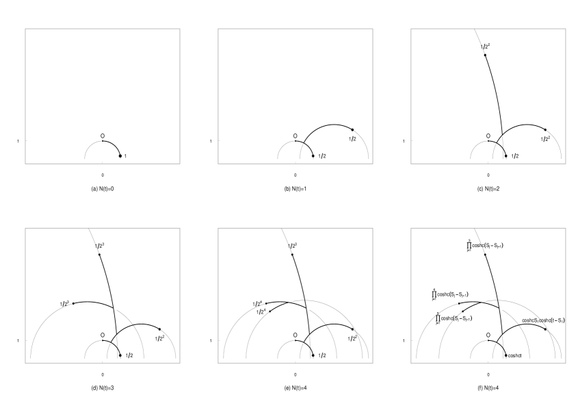
Figure 1: In (a), the trajectory of the unit-mass particle initially placed at the origin O 𝑂 O H 2 + superscript subscript 𝐻 2 H_{2}^{+} N ( t ) = 0 𝑁 𝑡 0 N(t)=0 N ( t ) = 1 , 2 , 3 , 4 𝑁 𝑡 1 2 3 4
N(t)=1,2,3,4
We assume that a unit-mass particle is placed at time t = 0 𝑡 0 t=0 O 𝑂 O H 2 + superscript subscript 𝐻 2 H_{2}^{+} H 2 + superscript subscript 𝐻 2 H_{2}^{+} 1 1 1 O 𝑂 O 1 / 2 1 2 1/2 c 𝑐 c 1
c = d s d t = 1 y ( d x d t ) 2 + ( d y d t ) 2 𝑐 d 𝑠 d 𝑡 1 𝑦 superscript d 𝑥 d 𝑡 2 superscript d 𝑦 d 𝑡 2 c=\frac{\mathrm{d}s}{\mathrm{d}t}=\frac{1}{y}\sqrt{\left(\frac{\mathrm{d}x}{\mathrm{d}t}\right)^{2}+\left(\frac{\mathrm{d}y}{\mathrm{d}t}\right)^{2}}
is assumed to be constant. For an Euclidean observer, the closer to the x 𝑥 x
A Poisson process of rate λ 𝜆 \lambda 1 k 𝑘 k 1 / 2 k 1 superscript 2 𝑘 1/2^{k} 1 / 2 k + 1 1 superscript 2 𝑘 1 1/2^{k+1} 1 / 2 k + 1 1 superscript 2 𝑘 1 1/2^{k+1} O 𝑂 O
Therefore, if no Poisson event occurs (i.e., { N ( t ) = 0 } 𝑁 𝑡 0 \{N(t)=0\} N ( t ) 𝑁 𝑡 N(t) [ 0 , t ] 0 𝑡 [0,t] t 𝑡 t O 𝑂 O η 0 ( t ) = c t subscript 𝜂 0 𝑡 𝑐 𝑡 \eta_{0}(t)=ct 1
If one Poisson event happens, at time S 1 < t subscript 𝑆 1 𝑡 S_{1}<t { N ( t ) = 1 } 𝑁 𝑡 1 \{N(t)=1\} t 𝑡 t 1 / 2 1 2 1/2 η 0 ( t ) = c t subscript 𝜂 0 𝑡 𝑐 𝑡 \eta_{0}(t)=ct 1 / 2 1 2 1/2 η 1 ( t ) subscript 𝜂 1 𝑡 \eta_{1}(t)
cosh η 1 ( t ) = cosh c S 1 cosh c ( t − S 1 ) , subscript 𝜂 1 𝑡 𝑐 subscript 𝑆 1 𝑐 𝑡 subscript 𝑆 1 \cosh\eta_{1}(t)=\cosh c\,S_{1}\cosh c(t-S_{1}), (3.1)
where in formula (3.1 2.4 1
If N ( t ) = n 𝑁 𝑡 𝑛 N(t)=n n + 1 𝑛 1 n+1 k 𝑘 k k = 0 , ⋯ n − 1 𝑘 0 ⋯ 𝑛 1
k=0,\cdots n-1 k 𝑘 k 1 / 2 k + 1 1 superscript 2 𝑘 1 1/2^{k+1} t 𝑡 t η k ( t ) subscript 𝜂 𝑘 𝑡 \eta_{k}(t) O 𝑂 O
cosh η k ( t ) = ∏ j = 1 k + 1 cosh c ( S j − S j − 1 ) , subscript 𝜂 𝑘 𝑡 superscript subscript product 𝑗 1 𝑘 1 𝑐 subscript 𝑆 𝑗 subscript 𝑆 𝑗 1 \cosh\eta_{k}(t)=\prod_{j=1}^{k+1}\cosh c(S_{j}-S_{j-1}),
where S 0 = 0 subscript 𝑆 0 0 S_{0}=0 S k + 1 = t subscript 𝑆 𝑘 1 𝑡 S_{k+1}=t S j subscript 𝑆 𝑗 S_{j} j = 1 , ⋯ k 𝑗 1 ⋯ 𝑘
j=1,\cdots k 1 / 2 n 1 superscript 2 𝑛 1/2^{n} t 𝑡 t O 𝑂 O
cosh η n ( t ) = ∏ j = 1 n + 1 cosh c ( S j − S j − 1 ) . subscript 𝜂 𝑛 𝑡 superscript subscript product 𝑗 1 𝑛 1 𝑐 subscript 𝑆 𝑗 subscript 𝑆 𝑗 1 \cosh\eta_{n}(t)=\prod_{j=1}^{n+1}\cosh c(S_{j}-S_{j-1}).
where S 0 = 0 subscript 𝑆 0 0 S_{0}=0 S n + 1 = t subscript 𝑆 𝑛 1 𝑡 S_{n+1}=t 1
In general, if the number of splits recorded is N ( t ) 𝑁 𝑡 N(t) N ( t ) + 1 𝑁 𝑡 1 N(t)+1 H 2 + superscript subscript 𝐻 2 H_{2}^{+} c m 𝑐 𝑚 cm t > 0 𝑡 0 t>0 η c m ( t ) subscript 𝜂 𝑐 𝑚 𝑡 \eta_{cm}(t)
cosh η c m ( t ) = ∑ k = 0 N ( t ) − 1 1 2 k + 1 ∏ j = 1 k + 1 cosh c ( S j − S j − 1 ) I { N ( t ) > 0 } + 1 2 N ( t ) ∏ j = 1 N ( t ) + 1 cosh c ( S j − S j − 1 ) , subscript 𝜂 𝑐 𝑚 𝑡 superscript subscript 𝑘 0 𝑁 𝑡 1 1 superscript 2 𝑘 1 superscript subscript product 𝑗 1 𝑘 1 𝑐 subscript 𝑆 𝑗 subscript 𝑆 𝑗 1 subscript 𝐼 𝑁 𝑡 0 1 superscript 2 𝑁 𝑡 superscript subscript product 𝑗 1 𝑁 𝑡 1 𝑐 subscript 𝑆 𝑗 subscript 𝑆 𝑗 1 \cosh\eta_{cm}(t)=\sum_{k=0}^{N(t)-1}\frac{1}{2^{k+1}}\prod_{j=1}^{k+1}\cosh c(S_{j}-S_{j-1})I_{\{N(t)>0\}}+\frac{1}{2^{N(t)}}\prod_{j=1}^{N(t)+1}\cosh c(S_{j}-S_{j-1}), (3.2)
where S 1 , S 2 … S N ( t ) subscript 𝑆 1 subscript 𝑆 2 … subscript 𝑆 𝑁 𝑡
S_{1},S_{2}\dots S_{N(t)} S 0 = 0 subscript 𝑆 0 0 S_{0}=0 S N ( t ) + 1 = t subscript 𝑆 𝑁 𝑡 1 𝑡 S_{N(t)+1}=t 3.2 t 𝑡 t
The assumption that the particles deviate on geodesic lines orthogonal to those joining the origin O 𝑂 O
Under the condition that N ( t ) = n 𝑁 𝑡 𝑛 N(t)=n t 𝑡 t
E { cosh η c m ( t ) | N ( t ) = n } 𝐸 conditional-set subscript 𝜂 𝑐 𝑚 𝑡 𝑁 𝑡 𝑛 \displaystyle E\{\cosh\eta_{cm}(t)|N(t)=n\} = \displaystyle= ∑ k = 0 n − 1 1 2 k + 1 ∏ j = 1 k + 1 cosh c ( S j − S j − 1 ) I { n > 0 } + 1 2 n ∏ j = 1 n + 1 cosh c ( S j − S j − 1 ) . superscript subscript 𝑘 0 𝑛 1 1 superscript 2 𝑘 1 superscript subscript product 𝑗 1 𝑘 1 𝑐 subscript 𝑆 𝑗 subscript 𝑆 𝑗 1 subscript 𝐼 𝑛 0 1 superscript 2 𝑛 superscript subscript product 𝑗 1 𝑛 1 𝑐 subscript 𝑆 𝑗 subscript 𝑆 𝑗 1 \displaystyle\sum_{k=0}^{n-1}\frac{1}{2^{k+1}}\prod_{j=1}^{k+1}\cosh c(S_{j}-S_{j-1})I_{\{n>0\}}+\frac{1}{2^{n}}\prod_{j=1}^{n+1}\cosh c(S_{j}-S_{j-1}).\;\;\; (3.3)
We observe that the n 𝑛 n S 1 , ⋯ , S n subscript 𝑆 1 ⋯ subscript 𝑆 𝑛
S_{1},\cdots,S_{n} N ( t ) = n 𝑁 𝑡 𝑛 N(t)=n
P r { S 1 ∈ d s 1 , ⋯ , S n ∈ d s n } = n ! t n d s 1 ⋯ d s n 𝑃 𝑟 formulae-sequence subscript 𝑆 1 d subscript 𝑠 1 ⋯
subscript 𝑆 𝑛 d subscript 𝑠 𝑛 𝑛 superscript 𝑡 𝑛 d subscript 𝑠 1 ⋯ d subscript 𝑠 𝑛 Pr\{S_{1}\in\mathrm{d}s_{1},\cdots,S_{n}\in\mathrm{d}s_{n}\}=\frac{n!}{t^{n}}\mathrm{d}s_{1}\cdots\mathrm{d}s_{n}
for 0 = s 0 < s 1 < ⋯ < s n + 1 = t 0 subscript 𝑠 0 subscript 𝑠 1 ⋯ subscript 𝑠 𝑛 1 𝑡 0=s_{0}<s_{1}<\cdots<s_{n+1}=t N ( t ) = n 𝑁 𝑡 𝑛 N(t)=n η k ( t ) subscript 𝜂 𝑘 𝑡 \eta_{k}(t) k 𝑘 k k = 0 , ⋯ n − 1 𝑘 0 ⋯ 𝑛 1
k=0,\cdots n-1
E { cosh η k ( t ) | N ( t ) = n } 𝐸 conditional-set subscript 𝜂 𝑘 𝑡 𝑁 𝑡 𝑛 \displaystyle E\{\cosh\eta_{k}(t)|N(t)=n\} = \displaystyle= n ! t n ∫ 0 t d s 1 ⋯ ∫ s k − 1 t d s k ⋯ ∫ s n − 1 t d s n ∏ j = 1 k + 1 cosh c ( s j − s j − 1 ) 𝑛 superscript 𝑡 𝑛 superscript subscript 0 𝑡 differential-d subscript 𝑠 1 ⋯ superscript subscript subscript 𝑠 𝑘 1 𝑡 differential-d subscript 𝑠 𝑘 ⋯ superscript subscript subscript 𝑠 𝑛 1 𝑡 differential-d subscript 𝑠 𝑛 superscript subscript product 𝑗 1 𝑘 1 𝑐 subscript 𝑠 𝑗 subscript 𝑠 𝑗 1 \displaystyle\frac{n!}{t^{n}}\int_{0}^{t}\mathrm{d}s_{1}\cdots\int_{s_{k-1}}^{t}\mathrm{d}s_{k}\cdots\int_{s_{n-1}}^{t}\mathrm{d}s_{n}\prod_{j=1}^{k+1}\cosh c(s_{j}-s_{j-1}) (3.4)
= \displaystyle= n ! t n ∫ 0 t d s 1 ⋯ ∫ s k − 1 t d s k ( t − s k ) n − k ( n − k ) ! ∏ j = 1 k + 1 cosh c ( s j − s j − 1 ) 𝑛 superscript 𝑡 𝑛 superscript subscript 0 𝑡 differential-d subscript 𝑠 1 ⋯ superscript subscript subscript 𝑠 𝑘 1 𝑡 differential-d subscript 𝑠 𝑘 superscript 𝑡 subscript 𝑠 𝑘 𝑛 𝑘 𝑛 𝑘 superscript subscript product 𝑗 1 𝑘 1 𝑐 subscript 𝑠 𝑗 subscript 𝑠 𝑗 1 \displaystyle\frac{n!}{t^{n}}\int_{0}^{t}\mathrm{d}s_{1}\cdots\int_{s_{k-1}}^{t}\mathrm{d}s_{k}\frac{(t-s_{k})^{n-k}}{(n-k)!}\prod_{j=1}^{k+1}\cosh c(s_{j}-s_{j-1})
= \displaystyle= n ! t n G n , k ( t ) , 𝑛 superscript 𝑡 𝑛 subscript 𝐺 𝑛 𝑘
𝑡 \displaystyle\frac{n!}{t^{n}}G_{n,k}(t),
and for k = n 𝑘 𝑛 k=n
E { cosh η n ( t ) | N ( t ) = n } 𝐸 conditional-set subscript 𝜂 𝑛 𝑡 𝑁 𝑡 𝑛 \displaystyle E\{\cosh\eta_{n}(t)|N(t)=n\} = \displaystyle= n ! t n ∫ 0 t d s 1 ⋯ ∫ s n − 1 t d s n ∏ j = 1 n + 1 cosh c ( s j − s j − 1 ) 𝑛 superscript 𝑡 𝑛 superscript subscript 0 𝑡 differential-d subscript 𝑠 1 ⋯ superscript subscript subscript 𝑠 𝑛 1 𝑡 differential-d subscript 𝑠 𝑛 superscript subscript product 𝑗 1 𝑛 1 𝑐 subscript 𝑠 𝑗 subscript 𝑠 𝑗 1 \displaystyle\frac{n!}{t^{n}}\int_{0}^{t}\mathrm{d}s_{1}\cdots\int_{s_{n-1}}^{t}\mathrm{d}s_{n}\prod_{j=1}^{n+1}\cosh c(s_{j}-s_{j-1}) (3.5)
= \displaystyle= n ! t n G n , n ( t ) . 𝑛 superscript 𝑡 𝑛 subscript 𝐺 𝑛 𝑛
𝑡 \displaystyle\frac{n!}{t^{n}}G_{n,n}(t).
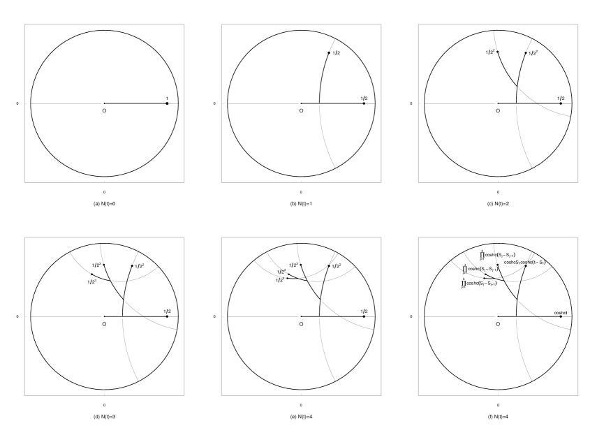
The branching process described above can be adapted to the Poincaré disk D 𝐷 D 2.6 2.7 D 𝐷 D H 2 + superscript subscript 𝐻 2 H_{2}^{+} 1 2
We restrict ourselves to the mean hyperbolic distance because this leads to fine explicit results. The analysis of the distribution of the hyperbolic distance, even in the case of a random motion of an individual particle that changes direction at all Poisson events, implies a much more complicated analysis and is almost intractable since multiple integrals of the form
E { e i α cosh η ( t ) | N ( t ) = n } = n ! t n ∫ 0 t d s 1 ⋯ ∫ s n − 1 t e i α ∏ j = 1 n + 1 cosh c ( s j − s j − 1 ) d s n 𝐸 conditional-set superscript 𝑒 𝑖 𝛼 𝜂 𝑡 𝑁 𝑡 𝑛 𝑛 superscript 𝑡 𝑛 superscript subscript 0 𝑡 differential-d subscript 𝑠 1 ⋯ superscript subscript subscript 𝑠 𝑛 1 𝑡 superscript 𝑒 𝑖 𝛼 superscript subscript product 𝑗 1 𝑛 1 𝑐 subscript 𝑠 𝑗 subscript 𝑠 𝑗 1 differential-d subscript 𝑠 𝑛 E\{e^{i\alpha\cosh\eta(t)}|N(t)=n\}=\frac{n!}{t^{n}}\int_{0}^{t}\mathrm{d}s_{1}\cdots\int_{s_{n-1}}^{t}e^{i\alpha\prod_{j=1}^{n+1}\cosh c(s_{j}-s_{j-1})}\mathrm{d}s_{n}
must be evaluated (see Cammarota and Orsingher [1 ] for details on this point).
Figure 2: Same trajectories as in Figure 1
4 Mean hyperbolic distance of the system of randomly moving and disintegrating particles: the Laplace transform approach
We are able to obtain the explicit form of the mean-value of (3.2
Theorem 4.1 .
The mean-value of the hyperbolic distance (3.2
E { cosh η c m ( t ) } 𝐸 subscript 𝜂 𝑐 𝑚 𝑡 \displaystyle E\{\cosh\eta_{cm}(t)\} = \displaystyle= 2 3 c 2 e − 3 2 2 λ t λ 2 + 2 4 c 2 { e − t 2 2 λ 2 + 2 4 c 2 3 λ 2 + 2 4 c 2 + 5 λ + e t 2 2 λ 2 + 2 4 c 2 3 λ 2 + 2 4 c 2 − 5 λ } superscript 2 3 superscript 𝑐 2 superscript 𝑒 3 superscript 2 2 𝜆 𝑡 superscript 𝜆 2 superscript 2 4 superscript 𝑐 2 superscript 𝑒 𝑡 superscript 2 2 superscript 𝜆 2 superscript 2 4 superscript 𝑐 2 3 superscript 𝜆 2 superscript 2 4 superscript 𝑐 2 5 𝜆 superscript 𝑒 𝑡 superscript 2 2 superscript 𝜆 2 superscript 2 4 superscript 𝑐 2 3 superscript 𝜆 2 superscript 2 4 superscript 𝑐 2 5 𝜆 \displaystyle\frac{2^{3}c^{2}e^{-\frac{3}{2^{2}}\lambda t}}{\sqrt{\lambda^{2}+2^{4}c^{2}}}\left\{\frac{e^{-\frac{t}{2^{2}}\sqrt{\lambda^{2}+2^{4}c^{2}}}}{3\sqrt{\lambda^{2}+2^{4}c^{2}}+5\lambda}+\frac{e^{\frac{t}{2^{2}}\sqrt{\lambda^{2}+2^{4}c^{2}}}}{3\sqrt{\lambda^{2}+2^{4}c^{2}}-5\lambda}\right\}
+ λ + 2 c 2 ( λ + 3 c ) e c t + λ − 2 c 2 ( λ − 3 c ) e − c t , t > 0 . 𝜆 2 𝑐 2 𝜆 3 𝑐 superscript 𝑒 𝑐 𝑡 𝜆 2 𝑐 2 𝜆 3 𝑐 superscript 𝑒 𝑐 𝑡 𝑡
0 \displaystyle+\frac{\lambda+2c}{2(\lambda+3c)}e^{ct}+\frac{\lambda-2c}{2(\lambda-3c)}e^{-ct},\hskip 85.35826ptt>0.
Proof
In view of (3.3 3.4 3.5
E { cosh η c m ( t ) | N ( t ) = n } 𝐸 conditional-set subscript 𝜂 𝑐 𝑚 𝑡 𝑁 𝑡 𝑛 \displaystyle E\{\cosh\eta_{cm}(t)|N(t)=n\} = \displaystyle= n ! t n ∑ k = 0 n − 1 1 2 k + 1 ∫ 0 t d s 1 ⋯ ∫ s n − 1 t d s n ∏ j = 1 k + 1 cosh c ( s j − s j − 1 ) 𝑛 superscript 𝑡 𝑛 superscript subscript 𝑘 0 𝑛 1 1 superscript 2 𝑘 1 superscript subscript 0 𝑡 differential-d subscript 𝑠 1 ⋯ superscript subscript subscript 𝑠 𝑛 1 𝑡 differential-d subscript 𝑠 𝑛 superscript subscript product 𝑗 1 𝑘 1 𝑐 subscript 𝑠 𝑗 subscript 𝑠 𝑗 1 \displaystyle\frac{n!}{t^{n}}\sum_{k=0}^{n-1}\frac{1}{2^{k+1}}\int_{0}^{t}\mathrm{d}s_{1}\cdots\int_{s_{n-1}}^{t}\mathrm{d}s_{n}\prod_{j=1}^{k+1}\cosh c(s_{j}-s_{j-1}) (4.4)
+ n ! t n 1 2 n ∫ 0 t d s 1 ⋯ ∫ s n − 1 t d s n ∏ j = 1 n + 1 cosh c ( s j − s j − 1 ) 𝑛 superscript 𝑡 𝑛 1 superscript 2 𝑛 superscript subscript 0 𝑡 differential-d subscript 𝑠 1 ⋯ superscript subscript subscript 𝑠 𝑛 1 𝑡 differential-d subscript 𝑠 𝑛 superscript subscript product 𝑗 1 𝑛 1 𝑐 subscript 𝑠 𝑗 subscript 𝑠 𝑗 1 \displaystyle+\frac{n!}{t^{n}}\frac{1}{2^{n}}\int_{0}^{t}\mathrm{d}s_{1}\cdots\int_{s_{n-1}}^{t}\mathrm{d}s_{n}\prod_{j=1}^{n+1}\cosh c(s_{j}-s_{j-1})
= \displaystyle= { n ! t n ∑ k = 0 n − 1 1 2 k + 1 G n , k ( t ) + n ! t n 1 2 n G n , n ( t ) , n ≥ 1 , G 0 , 0 ( t ) , n = 0 . cases 𝑛 superscript 𝑡 𝑛 superscript subscript 𝑘 0 𝑛 1 1 superscript 2 𝑘 1 subscript 𝐺 𝑛 𝑘
𝑡 𝑛 superscript 𝑡 𝑛 1 superscript 2 𝑛 subscript 𝐺 𝑛 𝑛
𝑡 𝑛
1 missing-subexpression missing-subexpression missing-subexpression subscript 𝐺 0 0
𝑡 𝑛
0 missing-subexpression \displaystyle\left\{\begin{array}[]{lr}\frac{n!}{t^{n}}\sum_{k=0}^{n-1}\frac{1}{2^{k+1}}G_{n,k}(t)+\frac{n!}{t^{n}}\frac{1}{2^{n}}G_{n,n}(t),\hskip 28.45274ptn\geq 1,\\
\\
G_{0,0}(t),\hskip 156.49014ptn=0.\end{array}\right.
Our task is therefore to study the Laplace transform,
∫ 0 ∞ e − μ t E { cosh η c m ( t ) } d t superscript subscript 0 superscript 𝑒 𝜇 𝑡 𝐸 subscript 𝜂 𝑐 𝑚 𝑡 differential-d 𝑡 \displaystyle\int_{0}^{\infty}e^{-\mu t}E\{\cosh\eta_{cm}(t)\}\mathrm{d}t = \displaystyle= ∫ 0 ∞ e − μ t ∑ n = 0 ∞ E { cosh η c m ( t ) | N ( t ) = n } P r { N ( t ) = n } d t superscript subscript 0 superscript 𝑒 𝜇 𝑡 superscript subscript 𝑛 0 𝐸 conditional-set subscript 𝜂 𝑐 𝑚 𝑡 𝑁 𝑡 𝑛 𝑃 𝑟 𝑁 𝑡 𝑛 d 𝑡 \displaystyle\int_{0}^{\infty}e^{-\mu t}\sum_{n=0}^{\infty}E\{\cosh\eta_{cm}(t)|N(t)=n\}Pr\{N(t)=n\}\mathrm{d}t (4.5)
= \displaystyle= ∑ n = 1 ∞ λ n ∑ k = 0 n − 1 1 2 k + 1 ∫ 0 ∞ e − ( λ + μ ) t G n , k ( t ) d t superscript subscript 𝑛 1 superscript 𝜆 𝑛 superscript subscript 𝑘 0 𝑛 1 1 superscript 2 𝑘 1 superscript subscript 0 superscript 𝑒 𝜆 𝜇 𝑡 subscript 𝐺 𝑛 𝑘
𝑡 differential-d 𝑡 \displaystyle\sum_{n=1}^{\infty}\lambda^{n}\sum_{k=0}^{n-1}\frac{1}{2^{k+1}}\int_{0}^{\infty}e^{-(\lambda+\mu)t}G_{n,k}(t)\mathrm{d}t
+ ∑ n = 0 ∞ λ n 2 n ∫ 0 ∞ e − ( λ + μ ) t G n , n ( t ) d t , superscript subscript 𝑛 0 superscript 𝜆 𝑛 superscript 2 𝑛 superscript subscript 0 superscript 𝑒 𝜆 𝜇 𝑡 subscript 𝐺 𝑛 𝑛
𝑡 differential-d 𝑡 \displaystyle+\sum_{n=0}^{\infty}\frac{\lambda^{n}}{2^{n}}\int_{0}^{\infty}e^{-(\lambda+\mu)t}G_{n,n}(t)\mathrm{d}t,
where μ > 0 𝜇 0 \mu>0 4.5 γ = λ + μ 𝛾 𝜆 𝜇 \gamma=\lambda+\mu c < γ 𝑐 𝛾 c<\gamma
∫ 0 ∞ e − γ t G n , k ( t ) d t superscript subscript 0 superscript 𝑒 𝛾 𝑡 subscript 𝐺 𝑛 𝑘
𝑡 differential-d 𝑡 \displaystyle\int_{0}^{\infty}e^{-\gamma t}G_{n,k}(t)\mathrm{d}t
= \displaystyle= ∫ 0 ∞ e − γ t { ∫ 0 t d s 1 ⋯ ∫ s k − 1 t d s k ( t − s k ) ( n − k ) ! n − k ∏ j = 1 k + 1 cosh c ( s j − s j − 1 ) } d t superscript subscript 0 superscript 𝑒 𝛾 𝑡 superscript subscript 0 𝑡 differential-d subscript 𝑠 1 ⋯ superscript subscript subscript 𝑠 𝑘 1 𝑡 differential-d subscript 𝑠 𝑘 superscript 𝑡 subscript 𝑠 𝑘 𝑛 𝑘 𝑛 𝑘 superscript subscript product 𝑗 1 𝑘 1 𝑐 subscript 𝑠 𝑗 subscript 𝑠 𝑗 1 differential-d 𝑡 \displaystyle\int_{0}^{\infty}e^{-\gamma t}\left\{\ \int_{0}^{t}\mathrm{d}s_{1}\cdots\int_{s_{k-1}}^{t}\mathrm{d}s_{k}\frac{(t-s_{k})}{(n-k)!}^{n-k}\;\;\prod_{j=1}^{k+1}\cosh c(s_{j}-s_{j-1})\right\}\mathrm{d}t
= \displaystyle= ∫ 0 ∞ d s 1 ∫ s 1 ∞ e − γ t d t { ∫ s 1 t d s 2 ⋯ ∫ s k − 1 t d s k ( t − s k ) ( n − k ) ! n − k ∏ j = 1 k + 1 cosh c ( s j − s j − 1 ) } superscript subscript 0 differential-d subscript 𝑠 1 superscript subscript subscript 𝑠 1 superscript 𝑒 𝛾 𝑡 differential-d 𝑡 superscript subscript subscript 𝑠 1 𝑡 differential-d subscript 𝑠 2 ⋯ superscript subscript subscript 𝑠 𝑘 1 𝑡 differential-d subscript 𝑠 𝑘 superscript 𝑡 subscript 𝑠 𝑘 𝑛 𝑘 𝑛 𝑘 superscript subscript product 𝑗 1 𝑘 1 𝑐 subscript 𝑠 𝑗 subscript 𝑠 𝑗 1 \displaystyle\int_{0}^{\infty}\mathrm{d}s_{1}\int_{s_{1}}^{\infty}e^{-\gamma t}\mathrm{d}t\left\{\int_{s_{1}}^{t}\mathrm{d}s_{2}\cdots\int_{s_{k-1}}^{t}\mathrm{d}s_{k}\frac{(t-s_{k})}{(n-k)!}^{n-k}\;\;\prod_{j=1}^{k+1}\cosh c(s_{j}-s_{j-1})\right\}
= \displaystyle= ∫ 0 ∞ d s 1 ∫ s 1 ∞ d s 2 ⋯ ∫ s k − 1 ∞ d s k ∏ j = 1 k cosh c ( s j − s j − 1 ) { ∫ s k ∞ e − γ t ( t − s k ) ( n − k ) ! n − k cosh c ( t − s k ) dt } superscript subscript 0 differential-d subscript 𝑠 1 superscript subscript subscript 𝑠 1 differential-d subscript 𝑠 2 ⋯ superscript subscript subscript 𝑠 𝑘 1 differential-d subscript 𝑠 𝑘 superscript subscript product 𝑗 1 𝑘 𝑐 subscript 𝑠 𝑗 subscript 𝑠 𝑗 1 superscript subscript subscript 𝑠 𝑘 superscript 𝑒 𝛾 𝑡 superscript 𝑡 subscript 𝑠 𝑘 𝑛 𝑘 𝑛 𝑘 𝑐 𝑡 subscript 𝑠 𝑘 dt \displaystyle\int_{0}^{\infty}\mathrm{d}s_{1}\int_{s_{1}}^{\infty}\mathrm{d}s_{2}\cdots\int_{s_{k-1}}^{\infty}\mathrm{d}s_{k}\prod_{j=1}^{k}\cosh c(s_{j}-s_{j-1})\left\{\int_{s_{k}}^{\infty}e^{-\gamma t}\frac{(t-s_{k})}{(n-k)!}^{n-k}\cosh c(t-s_{k})\mathrm{dt}\right\}
= \displaystyle= ∫ 0 ∞ d s 1 ⋯ ∫ s k − 2 ∞ d s k − 1 ∏ j = 1 k − 1 cosh c ( s j − s j − 1 ) ∫ s k − 1 ∞ e − γ s k cosh c ( s k − s k − 1 ) d s k superscript subscript 0 differential-d subscript 𝑠 1 ⋯ superscript subscript subscript 𝑠 𝑘 2 differential-d subscript 𝑠 𝑘 1 superscript subscript product 𝑗 1 𝑘 1 𝑐 subscript 𝑠 𝑗 subscript 𝑠 𝑗 1 superscript subscript subscript 𝑠 𝑘 1 superscript 𝑒 𝛾 subscript 𝑠 𝑘 𝑐 subscript 𝑠 𝑘 subscript 𝑠 𝑘 1 differential-d subscript 𝑠 𝑘 \displaystyle\int_{0}^{\infty}\mathrm{d}s_{1}\cdots\int_{s_{k-2}}^{\infty}\mathrm{d}s_{k-1}\prod_{j=1}^{k-1}\cosh c(s_{j}-s_{j-1})\int_{s_{k-1}}^{\infty}e^{-\gamma s_{k}}\cosh c(s_{k}-s_{k-1})\mathrm{d}s_{k}
× ∫ 0 ∞ e − γ w w n − k ( n − k ) ! cosh c w d w \displaystyle\times\int_{0}^{\infty}e^{-\gamma w}\frac{w^{n-k}}{(n-k)!}\cosh cw\;\mathrm{d}w
= \displaystyle= ( ∫ 0 ∞ e − γ w cosh c w ) k ∫ 0 ∞ e − γ w w n − k ( n − k ) ! cosh c w d w . superscript superscript subscript 0 superscript 𝑒 𝛾 𝑤 𝑐 𝑤 𝑘 superscript subscript 0 superscript 𝑒 𝛾 𝑤 superscript 𝑤 𝑛 𝑘 𝑛 𝑘 𝑐 𝑤 d 𝑤 \displaystyle\left(\int_{0}^{\infty}e^{-\gamma w}\cosh cw\right)^{k}\int_{0}^{\infty}e^{-\gamma w}\frac{w^{n-k}}{(n-k)!}\cosh cw\;\mathrm{d}w.
In the last step above the change of variable s j − s j − 1 = w j subscript 𝑠 𝑗 subscript 𝑠 𝑗 1 subscript 𝑤 𝑗 s_{j}-s_{j-1}=w_{j} k 𝑘 k k = n 𝑘 𝑛 k=n
∫ 0 ∞ e − γ t G n , n ( t ) d t = ( ∫ 0 ∞ e − γ w cosh c w d w ) n + 1 . superscript subscript 0 superscript 𝑒 𝛾 𝑡 subscript 𝐺 𝑛 𝑛
𝑡 differential-d 𝑡 superscript superscript subscript 0 superscript 𝑒 𝛾 𝑤 𝑐 𝑤 d 𝑤 𝑛 1 \int_{0}^{\infty}e^{-\gamma t}G_{n,n}(t)\mathrm{d}t=\left(\int_{0}^{\infty}e^{-\gamma w}\cosh cw\;\mathrm{d}w\right)^{n+1}.
Since
∫ 0 ∞ e − γ w cosh c w d w superscript subscript 0 superscript 𝑒 𝛾 𝑤 𝑐 𝑤 d 𝑤 \displaystyle\int_{0}^{\infty}e^{-\gamma w}\cosh cw\;\mathrm{d}w = \displaystyle= γ γ 2 − c 2 , 𝛾 superscript 𝛾 2 superscript 𝑐 2 \displaystyle\frac{\gamma}{\gamma^{2}-c^{2}},
∫ 0 ∞ e − γ w w n − k ( n − k ) ! cosh c w d w superscript subscript 0 superscript 𝑒 𝛾 𝑤 superscript 𝑤 𝑛 𝑘 𝑛 𝑘 𝑐 𝑤 d 𝑤 \displaystyle\int_{0}^{\infty}e^{-\gamma w}\frac{w^{n-k}}{(n-k)!}\cosh cw\;\mathrm{d}w = \displaystyle= 1 2 [ 1 ( γ − c ) n − k + 1 + 1 ( γ + c ) n − k + 1 ] , 1 2 delimited-[] 1 superscript 𝛾 𝑐 𝑛 𝑘 1 1 superscript 𝛾 𝑐 𝑛 𝑘 1 \displaystyle\frac{1}{2}\left[\frac{1}{(\gamma-c)^{n-k+1}}+\frac{1}{(\gamma+c)^{n-k+1}}\right],
we have that
∫ 0 ∞ e − μ t E { cosh η c m ( t ) } d t superscript subscript 0 superscript 𝑒 𝜇 𝑡 𝐸 subscript 𝜂 𝑐 𝑚 𝑡 differential-d 𝑡 \displaystyle\int_{0}^{\infty}e^{-\mu t}E\{\cosh\eta_{cm}(t)\}\mathrm{d}t (4.6)
= \displaystyle= ∑ n = 1 ∞ λ n ∑ k = 0 n − 1 1 2 k + 1 ( γ γ 2 − c 2 ) k 1 2 [ 1 ( γ − c ) n − k + 1 + 1 ( γ + c ) n − k + 1 ] superscript subscript 𝑛 1 superscript 𝜆 𝑛 superscript subscript 𝑘 0 𝑛 1 1 superscript 2 𝑘 1 superscript 𝛾 superscript 𝛾 2 superscript 𝑐 2 𝑘 1 2 delimited-[] 1 superscript 𝛾 𝑐 𝑛 𝑘 1 1 superscript 𝛾 𝑐 𝑛 𝑘 1 \displaystyle\sum_{n=1}^{\infty}\lambda^{n}\sum_{k=0}^{n-1}\frac{1}{2^{k+1}}\left(\frac{\gamma}{\gamma^{2}-c^{2}}\right)^{k}\frac{1}{2}\left[\frac{1}{(\gamma-c)^{n-k+1}}+\frac{1}{(\gamma+c)^{n-k+1}}\right]
+ ∑ n = 0 ∞ ( λ 2 ) n ( γ γ 2 − c 2 ) n + 1 superscript subscript 𝑛 0 superscript 𝜆 2 𝑛 superscript 𝛾 superscript 𝛾 2 superscript 𝑐 2 𝑛 1 \displaystyle+\sum_{n=0}^{\infty}\left(\frac{\lambda}{2}\right)^{n}\left(\frac{\gamma}{\gamma^{2}-c^{2}}\right)^{n+1}
= \displaystyle= 1 2 2 ∑ n = 1 ∞ λ n { 1 ( γ − c ) n + 1 ∑ k = 0 n − 1 [ γ 2 ( γ + c ) ] k + 1 ( γ + c ) n + 1 ∑ k = 0 n − 1 [ γ 2 ( γ − c ) ] k } 1 superscript 2 2 superscript subscript 𝑛 1 superscript 𝜆 𝑛 1 superscript 𝛾 𝑐 𝑛 1 superscript subscript 𝑘 0 𝑛 1 superscript delimited-[] 𝛾 2 𝛾 𝑐 𝑘 1 superscript 𝛾 𝑐 𝑛 1 superscript subscript 𝑘 0 𝑛 1 superscript delimited-[] 𝛾 2 𝛾 𝑐 𝑘 \displaystyle\frac{1}{2^{2}}\sum_{n=1}^{\infty}\lambda^{n}\left\{\frac{1}{(\gamma-c)^{n+1}}\sum_{k=0}^{n-1}\left[\frac{\gamma}{2(\gamma+c)}\right]^{k}+\frac{1}{(\gamma+c)^{n+1}}\sum_{k=0}^{n-1}\left[\frac{\gamma}{2(\gamma-c)}\right]^{k}\right\}
+ 2 γ 2 γ 2 − 2 c 2 − γ λ , 2 𝛾 2 superscript 𝛾 2 2 superscript 𝑐 2 𝛾 𝜆 \displaystyle+\frac{2\gamma}{2\gamma^{2}-2c^{2}-\gamma\lambda},
where the last sum converges if μ 𝜇 \mu 2 c 2 < λ 2 + 2 μ 2 + 3 λ μ 2 superscript 𝑐 2 superscript 𝜆 2 2 superscript 𝜇 2 3 𝜆 𝜇 2c^{2}<\lambda^{2}+2\mu^{2}+3\lambda\mu 4.6
∑ n = 1 ∞ λ n { 1 ( γ − c ) n + 1 ∑ k = 0 n − 1 [ γ 2 ( γ + c ) ] k + 1 ( γ + c ) n + 1 ∑ k = 0 n − 1 [ γ 2 ( γ − c ) ] k } superscript subscript 𝑛 1 superscript 𝜆 𝑛 1 superscript 𝛾 𝑐 𝑛 1 superscript subscript 𝑘 0 𝑛 1 superscript delimited-[] 𝛾 2 𝛾 𝑐 𝑘 1 superscript 𝛾 𝑐 𝑛 1 superscript subscript 𝑘 0 𝑛 1 superscript delimited-[] 𝛾 2 𝛾 𝑐 𝑘 \displaystyle\sum_{n=1}^{\infty}\lambda^{n}\left\{\frac{1}{(\gamma-c)^{n+1}}\sum_{k=0}^{n-1}\left[\frac{\gamma}{2(\gamma+c)}\right]^{k}+\frac{1}{(\gamma+c)^{n+1}}\sum_{k=0}^{n-1}\left[\frac{\gamma}{2(\gamma-c)}\right]^{k}\right\} (4.7)
= \displaystyle= 1 γ − c ∑ k = 0 ∞ [ γ 2 ( γ + c ) ] k ∑ n = k + 1 ∞ ( λ γ − c ) n + 1 γ + c ∑ k = 0 ∞ [ γ 2 ( γ − c ) ] k ∑ n = k + 1 ∞ ( λ γ + c ) n 1 𝛾 𝑐 superscript subscript 𝑘 0 superscript delimited-[] 𝛾 2 𝛾 𝑐 𝑘 superscript subscript 𝑛 𝑘 1 superscript 𝜆 𝛾 𝑐 𝑛 1 𝛾 𝑐 superscript subscript 𝑘 0 superscript delimited-[] 𝛾 2 𝛾 𝑐 𝑘 superscript subscript 𝑛 𝑘 1 superscript 𝜆 𝛾 𝑐 𝑛 \displaystyle\frac{1}{\gamma-c}\sum_{k=0}^{\infty}\left[\frac{\gamma}{2(\gamma+c)}\right]^{k}\sum_{n=k+1}^{\infty}\left(\frac{\lambda}{\gamma-c}\right)^{n}+\frac{1}{\gamma+c}\sum_{k=0}^{\infty}\left[\frac{\gamma}{2(\gamma-c)}\right]^{k}\sum_{n=k+1}^{\infty}\left(\frac{\lambda}{\gamma+c}\right)^{n}
= \displaystyle= 1 γ − c ∑ k = 0 ∞ [ γ 2 ( γ + c ) ] k ( λ γ − c ) k + 1 ∑ r = 0 ∞ ( λ γ − c ) r 1 𝛾 𝑐 superscript subscript 𝑘 0 superscript delimited-[] 𝛾 2 𝛾 𝑐 𝑘 superscript 𝜆 𝛾 𝑐 𝑘 1 superscript subscript 𝑟 0 superscript 𝜆 𝛾 𝑐 𝑟 \displaystyle\frac{1}{\gamma-c}\sum_{k=0}^{\infty}\left[\frac{\gamma}{2(\gamma+c)}\right]^{k}\left(\frac{\lambda}{\gamma-c}\right)^{k+1}\sum_{r=0}^{\infty}\left(\frac{\lambda}{\gamma-c}\right)^{r}
+ 1 γ + c ∑ k = 0 ∞ [ γ 2 ( γ − c ) ] k ( λ γ + c ) k + 1 ∑ r = 0 ∞ ( λ γ + c ) r 1 𝛾 𝑐 superscript subscript 𝑘 0 superscript delimited-[] 𝛾 2 𝛾 𝑐 𝑘 superscript 𝜆 𝛾 𝑐 𝑘 1 superscript subscript 𝑟 0 superscript 𝜆 𝛾 𝑐 𝑟 \displaystyle+\frac{1}{\gamma+c}\sum_{k=0}^{\infty}\left[\frac{\gamma}{2(\gamma-c)}\right]^{k}\left(\frac{\lambda}{\gamma+c}\right)^{k+1}\sum_{r=0}^{\infty}\left(\frac{\lambda}{\gamma+c}\right)^{r}
= \displaystyle= λ ( γ − c ) 2 ∑ k = 0 ∞ [ γ λ 2 ( γ 2 − c 2 ) ] k γ − c γ − c − λ + λ ( γ + c ) 2 ∑ k = 0 ∞ [ γ λ 2 ( γ 2 − c 2 ) ] k γ + c γ + c − λ 𝜆 superscript 𝛾 𝑐 2 superscript subscript 𝑘 0 superscript delimited-[] 𝛾 𝜆 2 superscript 𝛾 2 superscript 𝑐 2 𝑘 𝛾 𝑐 𝛾 𝑐 𝜆 𝜆 superscript 𝛾 𝑐 2 superscript subscript 𝑘 0 superscript delimited-[] 𝛾 𝜆 2 superscript 𝛾 2 superscript 𝑐 2 𝑘 𝛾 𝑐 𝛾 𝑐 𝜆 \displaystyle\frac{\lambda}{(\gamma-c)^{2}}\sum_{k=0}^{\infty}\left[\frac{\gamma\lambda}{2(\gamma^{2}-c^{2})}\right]^{k}\frac{\gamma-c}{\gamma-c-\lambda}+\frac{\lambda}{(\gamma+c)^{2}}\sum_{k=0}^{\infty}\left[\frac{\gamma\lambda}{2(\gamma^{2}-c^{2})}\right]^{k}\frac{\gamma+c}{\gamma+c-\lambda}
= \displaystyle= λ [ 1 γ − c 1 γ − c − λ + 1 γ + c 1 γ + c − λ ] ∑ k = 0 ∞ [ γ λ 2 ( γ 2 − c 2 ) ] k 𝜆 delimited-[] 1 𝛾 𝑐 1 𝛾 𝑐 𝜆 1 𝛾 𝑐 1 𝛾 𝑐 𝜆 superscript subscript 𝑘 0 superscript delimited-[] 𝛾 𝜆 2 superscript 𝛾 2 superscript 𝑐 2 𝑘 \displaystyle\lambda\left[\frac{1}{\gamma-c}\;\frac{1}{\gamma-c-\lambda}+\frac{1}{\gamma+c}\;\frac{1}{\gamma+c-\lambda}\right]\sum_{k=0}^{\infty}\left[\frac{\gamma\lambda}{2(\gamma^{2}-c^{2})}\right]^{k}
= \displaystyle= λ [ 1 γ − c 1 γ − c − λ + 1 γ + c 1 γ + c − λ ] 2 ( γ 2 − c 2 ) 2 γ 2 − 2 c 2 − γ λ . 𝜆 delimited-[] 1 𝛾 𝑐 1 𝛾 𝑐 𝜆 1 𝛾 𝑐 1 𝛾 𝑐 𝜆 2 superscript 𝛾 2 superscript 𝑐 2 2 superscript 𝛾 2 2 superscript 𝑐 2 𝛾 𝜆 \displaystyle\lambda\left[\frac{1}{\gamma-c}\;\frac{1}{\gamma-c-\lambda}+\frac{1}{\gamma+c}\;\frac{1}{\gamma+c-\lambda}\right]\frac{2(\gamma^{2}-c^{2})}{2\gamma^{2}-2c^{2}-\gamma\lambda}.
The inversion of the Laplace transform is made possible by suitably rearranging the expression (4.7
∫ 0 ∞ e − μ t E { cosh η c m ( t ) } d t superscript subscript 0 superscript 𝑒 𝜇 𝑡 𝐸 subscript 𝜂 𝑐 𝑚 𝑡 differential-d 𝑡 \displaystyle\int_{0}^{\infty}e^{-\mu t}E\{\cosh\eta_{cm}(t)\}\mathrm{d}t (4.8)
= \displaystyle= λ 2 [ 1 γ − c 1 γ − c − λ + 1 γ + c 1 γ + c − λ ] γ 2 − c 2 2 γ 2 − 2 c 2 − γ λ + 2 γ 2 γ 2 − 2 c 2 − γ λ 𝜆 2 delimited-[] 1 𝛾 𝑐 1 𝛾 𝑐 𝜆 1 𝛾 𝑐 1 𝛾 𝑐 𝜆 superscript 𝛾 2 superscript 𝑐 2 2 superscript 𝛾 2 2 superscript 𝑐 2 𝛾 𝜆 2 𝛾 2 superscript 𝛾 2 2 superscript 𝑐 2 𝛾 𝜆 \displaystyle\frac{\lambda}{2}\left[\frac{1}{\gamma-c}\;\frac{1}{\gamma-c-\lambda}+\frac{1}{\gamma+c}\;\frac{1}{\gamma+c-\lambda}\right]\frac{\gamma^{2}-c^{2}}{2\gamma^{2}-2c^{2}-\gamma\lambda}+\frac{2\gamma}{2\gamma^{2}-2c^{2}-\gamma\lambda}
= \displaystyle= λ 2 [ 1 λ + μ − c 1 μ − c + 1 λ + μ + c 1 μ + c ] ( λ + μ ) 2 − c 2 λ 2 + 2 μ 2 + 3 λ μ − 2 c 2 + 2 λ + 2 μ λ 2 + 2 μ 2 + 3 λ μ − 2 c 2 𝜆 2 delimited-[] 1 𝜆 𝜇 𝑐 1 𝜇 𝑐 1 𝜆 𝜇 𝑐 1 𝜇 𝑐 superscript 𝜆 𝜇 2 superscript 𝑐 2 superscript 𝜆 2 2 superscript 𝜇 2 3 𝜆 𝜇 2 superscript 𝑐 2 2 𝜆 2 𝜇 superscript 𝜆 2 2 superscript 𝜇 2 3 𝜆 𝜇 2 superscript 𝑐 2 \displaystyle\frac{\lambda}{2}\left[\frac{1}{\lambda+\mu-c}\;\frac{1}{\mu-c}+\frac{1}{\lambda+\mu+c}\;\frac{1}{\mu+c}\right]\frac{(\lambda+\mu)^{2}-c^{2}}{\lambda^{2}+2\mu^{2}+3\lambda\mu-2c^{2}}+\frac{2\lambda+2\mu}{\lambda^{2}+2\mu^{2}+3\lambda\mu-2c^{2}}
= \displaystyle= λ 2 [ λ + μ + c μ − c + λ + μ − c μ + c ] 1 λ 2 + 2 μ 2 + 3 λ μ − 2 c 2 + 2 λ + 2 μ λ 2 + 2 μ 2 + 3 λ μ − 2 c 2 . 𝜆 2 delimited-[] 𝜆 𝜇 𝑐 𝜇 𝑐 𝜆 𝜇 𝑐 𝜇 𝑐 1 superscript 𝜆 2 2 superscript 𝜇 2 3 𝜆 𝜇 2 superscript 𝑐 2 2 𝜆 2 𝜇 superscript 𝜆 2 2 superscript 𝜇 2 3 𝜆 𝜇 2 superscript 𝑐 2 \displaystyle\frac{\lambda}{2}\left[\frac{\lambda+\mu+c}{\mu-c}+\frac{\lambda+\mu-c}{\mu+c}\right]\frac{1}{\lambda^{2}+2\mu^{2}+3\lambda\mu-2c^{2}}+\frac{2\lambda+2\mu}{\lambda^{2}+2\mu^{2}+3\lambda\mu-2c^{2}}.
By means of the decomposition
2 μ 2 + 3 λ μ + λ 2 − 2 c 2 = 2 [ μ + 3 λ − λ 2 + 2 4 c 2 2 2 ] [ μ + 3 λ + λ 2 + 2 4 c 2 2 2 ] , 2 superscript 𝜇 2 3 𝜆 𝜇 superscript 𝜆 2 2 superscript 𝑐 2 2 delimited-[] 𝜇 3 𝜆 superscript 𝜆 2 superscript 2 4 superscript 𝑐 2 superscript 2 2 delimited-[] 𝜇 3 𝜆 superscript 𝜆 2 superscript 2 4 superscript 𝑐 2 superscript 2 2 2\mu^{2}+3\lambda\mu+\lambda^{2}-2c^{2}=2\left[\mu+\frac{3\lambda-\sqrt{\lambda^{2}+2^{4}c^{2}}}{2^{2}}\right]\left[\mu+\frac{3\lambda+\sqrt{\lambda^{2}+2^{4}c^{2}}}{2^{2}}\right],
the expression (4.8
∫ 0 ∞ e − μ t E { cosh η c m ( t ) } d t superscript subscript 0 superscript 𝑒 𝜇 𝑡 𝐸 subscript 𝜂 𝑐 𝑚 𝑡 differential-d 𝑡 \displaystyle\int_{0}^{\infty}e^{-\mu t}E\{\cosh\eta_{cm}(t)\}\mathrm{d}t (4.9)
= \displaystyle= λ 2 2 1 [ μ + 3 λ − λ 2 + 2 4 c 2 2 2 ] [ μ + 3 λ + λ 2 + 2 4 c 2 2 2 ] [ 2 + λ + 2 c μ − c + λ − 2 c μ + c ] 𝜆 superscript 2 2 1 delimited-[] 𝜇 3 𝜆 superscript 𝜆 2 superscript 2 4 superscript 𝑐 2 superscript 2 2 delimited-[] 𝜇 3 𝜆 superscript 𝜆 2 superscript 2 4 superscript 𝑐 2 superscript 2 2 delimited-[] 2 𝜆 2 𝑐 𝜇 𝑐 𝜆 2 𝑐 𝜇 𝑐 \displaystyle\frac{\lambda}{2^{2}}\frac{1}{\left[\mu+\frac{3\lambda-\sqrt{\lambda^{2}+2^{4}c^{2}}}{2^{2}}\right]\left[\mu+\frac{3\lambda+\sqrt{\lambda^{2}+2^{4}c^{2}}}{2^{2}}\right]}\left[2+\frac{\lambda+2c}{\mu-c}+\frac{\lambda-2c}{\mu+c}\right]
+ 3 2 λ + λ 2 + 2 μ 2 [ μ + 3 λ − λ 2 + 2 4 c 2 2 2 ] [ μ + 3 λ + λ 2 + 2 4 c 2 2 2 ] 3 2 𝜆 𝜆 2 2 𝜇 2 delimited-[] 𝜇 3 𝜆 superscript 𝜆 2 superscript 2 4 superscript 𝑐 2 superscript 2 2 delimited-[] 𝜇 3 𝜆 superscript 𝜆 2 superscript 2 4 superscript 𝑐 2 superscript 2 2 \displaystyle+\frac{\frac{3}{2}\lambda+\frac{\lambda}{2}+2\mu}{2\left[\mu+\frac{3\lambda-\sqrt{\lambda^{2}+2^{4}c^{2}}}{2^{2}}\right]\left[\mu+\frac{3\lambda+\sqrt{\lambda^{2}+2^{4}c^{2}}}{2^{2}}\right]}
= \displaystyle= [ 1 μ + 3 λ − λ 2 + 2 4 c 2 2 2 − 1 μ + 3 λ + λ 2 + 2 4 c 2 2 2 ] λ 2 2 2 λ 2 + 2 4 c 2 [ 2 + λ + 2 c μ − c + λ − 2 c μ + c ] delimited-[] 1 𝜇 3 𝜆 superscript 𝜆 2 superscript 2 4 superscript 𝑐 2 superscript 2 2 1 𝜇 3 𝜆 superscript 𝜆 2 superscript 2 4 superscript 𝑐 2 superscript 2 2 𝜆 superscript 2 2 2 superscript 𝜆 2 superscript 2 4 superscript 𝑐 2 delimited-[] 2 𝜆 2 𝑐 𝜇 𝑐 𝜆 2 𝑐 𝜇 𝑐 \displaystyle\left[\frac{1}{\mu+\frac{3\lambda-\sqrt{\lambda^{2}+2^{4}c^{2}}}{2^{2}}}-\frac{1}{\mu+\frac{3\lambda+\sqrt{\lambda^{2}+2^{4}c^{2}}}{2^{2}}}\right]\frac{\lambda}{2^{2}}\frac{2}{\sqrt{\lambda^{2}+2^{4}c^{2}}}\left[2+\frac{\lambda+2c}{\mu-c}+\frac{\lambda-2c}{\mu+c}\right]
+ [ 1 μ + 3 λ − λ 2 + 2 4 c 2 2 2 + 1 μ + 3 λ + λ 2 + 2 4 c 2 2 2 ] 3 2 λ + λ 2 + 2 μ 2 ( 2 μ + 3 2 λ ) delimited-[] 1 𝜇 3 𝜆 superscript 𝜆 2 superscript 2 4 superscript 𝑐 2 superscript 2 2 1 𝜇 3 𝜆 superscript 𝜆 2 superscript 2 4 superscript 𝑐 2 superscript 2 2 3 2 𝜆 𝜆 2 2 𝜇 2 2 𝜇 3 2 𝜆 \displaystyle+\left[\frac{1}{\mu+\frac{3\lambda-\sqrt{\lambda^{2}+2^{4}c^{2}}}{2^{2}}}+\frac{1}{\mu+\frac{3\lambda+\sqrt{\lambda^{2}+2^{4}c^{2}}}{2^{2}}}\right]\frac{\frac{3}{2}\lambda+\frac{\lambda}{2}+2\mu}{2\left(2\mu+\frac{3}{2}\lambda\right)}
= \displaystyle= [ 1 μ + 3 λ − λ 2 + 2 4 c 2 2 2 − 1 μ + 3 λ + λ 2 + 2 4 c 2 2 2 ] λ λ 2 + 2 4 c 2 + 1 2 [ 1 μ + 3 λ − λ 2 + 2 4 c 2 2 2 + 1 μ + 3 λ + λ 2 + 2 4 c 2 2 2 ] delimited-[] 1 𝜇 3 𝜆 superscript 𝜆 2 superscript 2 4 superscript 𝑐 2 superscript 2 2 1 𝜇 3 𝜆 superscript 𝜆 2 superscript 2 4 superscript 𝑐 2 superscript 2 2 𝜆 superscript 𝜆 2 superscript 2 4 superscript 𝑐 2 1 2 delimited-[] 1 𝜇 3 𝜆 superscript 𝜆 2 superscript 2 4 superscript 𝑐 2 superscript 2 2 1 𝜇 3 𝜆 superscript 𝜆 2 superscript 2 4 superscript 𝑐 2 superscript 2 2 \displaystyle\left[\frac{1}{\mu+\frac{3\lambda-\sqrt{\lambda^{2}+2^{4}c^{2}}}{2^{2}}}-\frac{1}{\mu+\frac{3\lambda+\sqrt{\lambda^{2}+2^{4}c^{2}}}{2^{2}}}\right]\frac{\lambda}{\sqrt{\lambda^{2}+2^{4}c^{2}}}+\frac{1}{2}\left[\frac{1}{\mu+\frac{3\lambda-\sqrt{\lambda^{2}+2^{4}c^{2}}}{2^{2}}}+\frac{1}{\mu+\frac{3\lambda+\sqrt{\lambda^{2}+2^{4}c^{2}}}{2^{2}}}\right]
+ [ 1 μ + 3 λ − λ 2 + 2 4 c 2 2 2 − 1 μ + 3 λ + λ 2 + 2 4 c 2 2 2 ] λ 2 λ 2 + 2 4 c 2 [ λ + 2 c μ − c + λ − 2 c μ + c ] delimited-[] 1 𝜇 3 𝜆 superscript 𝜆 2 superscript 2 4 superscript 𝑐 2 superscript 2 2 1 𝜇 3 𝜆 superscript 𝜆 2 superscript 2 4 superscript 𝑐 2 superscript 2 2 𝜆 2 superscript 𝜆 2 superscript 2 4 superscript 𝑐 2 delimited-[] 𝜆 2 𝑐 𝜇 𝑐 𝜆 2 𝑐 𝜇 𝑐 \displaystyle+\left[\frac{1}{\mu+\frac{3\lambda-\sqrt{\lambda^{2}+2^{4}c^{2}}}{2^{2}}}-\frac{1}{\mu+\frac{3\lambda+\sqrt{\lambda^{2}+2^{4}c^{2}}}{2^{2}}}\right]\frac{\lambda}{2\sqrt{\lambda^{2}+2^{4}c^{2}}}\left[\frac{\lambda+2c}{\mu-c}+\frac{\lambda-2c}{\mu+c}\right]
+ [ 1 μ + 3 λ − λ 2 + 2 4 c 2 2 2 + 1 μ + 3 λ + λ 2 + 2 4 c 2 2 2 ] λ 2 2 ( 2 μ + 3 2 λ ) . delimited-[] 1 𝜇 3 𝜆 superscript 𝜆 2 superscript 2 4 superscript 𝑐 2 superscript 2 2 1 𝜇 3 𝜆 superscript 𝜆 2 superscript 2 4 superscript 𝑐 2 superscript 2 2 𝜆 superscript 2 2 2 𝜇 3 2 𝜆 \displaystyle+\left[\frac{1}{\mu+\frac{3\lambda-\sqrt{\lambda^{2}+2^{4}c^{2}}}{2^{2}}}+\frac{1}{\mu+\frac{3\lambda+\sqrt{\lambda^{2}+2^{4}c^{2}}}{2^{2}}}\right]\frac{\lambda}{2^{2}(2\mu+\frac{3}{2}\lambda)}.
It is now a simple matter to invert the Laplace transform (4.9
E { cosh η c m ( t ) } 𝐸 subscript 𝜂 𝑐 𝑚 𝑡 \displaystyle E\{\cosh\eta_{cm}(t)\} (4.10)
= \displaystyle= [ 1 2 + λ λ 2 + 2 4 c 2 ] e − t 3 λ − λ 2 + 2 4 c 2 2 2 + [ 1 2 − λ λ 2 + 2 4 c 2 ] e − t 3 λ + λ 2 + 2 4 c 2 2 2 delimited-[] 1 2 𝜆 superscript 𝜆 2 superscript 2 4 superscript 𝑐 2 superscript 𝑒 𝑡 3 𝜆 superscript 𝜆 2 superscript 2 4 superscript 𝑐 2 superscript 2 2 delimited-[] 1 2 𝜆 superscript 𝜆 2 superscript 2 4 superscript 𝑐 2 superscript 𝑒 𝑡 3 𝜆 superscript 𝜆 2 superscript 2 4 superscript 𝑐 2 superscript 2 2 \displaystyle\left[\frac{1}{2}+\frac{\lambda}{\sqrt{\lambda^{2}+2^{4}c^{2}}}\right]e^{-t\frac{3\lambda-\sqrt{\lambda^{2}+2^{4}c^{2}}}{2^{2}}}+\left[\frac{1}{2}-\frac{\lambda}{\sqrt{\lambda^{2}+2^{4}c^{2}}}\right]e^{-t\frac{3\lambda+\sqrt{\lambda^{2}+2^{4}c^{2}}}{2^{2}}}
+ λ ( λ + 2 c ) 2 λ 2 + 2 4 c 2 [ ∫ 0 t e c s e − ( t − s ) 3 λ − λ 2 + 2 4 c 2 2 2 d s − ∫ 0 t e c s e − ( t − s ) 3 λ + λ 2 + 2 4 c 2 2 2 d s ] 𝜆 𝜆 2 𝑐 2 superscript 𝜆 2 superscript 2 4 superscript 𝑐 2 delimited-[] superscript subscript 0 𝑡 superscript 𝑒 𝑐 𝑠 superscript 𝑒 𝑡 𝑠 3 𝜆 superscript 𝜆 2 superscript 2 4 superscript 𝑐 2 superscript 2 2 differential-d 𝑠 superscript subscript 0 𝑡 superscript 𝑒 𝑐 𝑠 superscript 𝑒 𝑡 𝑠 3 𝜆 superscript 𝜆 2 superscript 2 4 superscript 𝑐 2 superscript 2 2 differential-d 𝑠 \displaystyle+\frac{\lambda(\lambda+2c)}{2\sqrt{\lambda^{2}+2^{4}c^{2}}}\left[\int_{0}^{t}e^{cs}e^{-(t-s)\frac{3\lambda-\sqrt{\lambda^{2}+2^{4}c^{2}}}{2^{2}}}\mathrm{d}s-\int_{0}^{t}e^{cs}e^{-(t-s)\frac{3\lambda+\sqrt{\lambda^{2}+2^{4}c^{2}}}{2^{2}}}\mathrm{d}s\right]
+ λ ( λ − 2 c ) 2 λ 2 + 2 4 c 2 [ ∫ 0 t e − c s e − ( t − s ) 3 λ − λ 2 + 2 4 c 2 2 2 d s − ∫ 0 t e − c s e − ( t − s ) 3 λ + λ 2 + 2 4 c 2 2 2 d s ] 𝜆 𝜆 2 𝑐 2 superscript 𝜆 2 superscript 2 4 superscript 𝑐 2 delimited-[] superscript subscript 0 𝑡 superscript 𝑒 𝑐 𝑠 superscript 𝑒 𝑡 𝑠 3 𝜆 superscript 𝜆 2 superscript 2 4 superscript 𝑐 2 superscript 2 2 differential-d 𝑠 superscript subscript 0 𝑡 superscript 𝑒 𝑐 𝑠 superscript 𝑒 𝑡 𝑠 3 𝜆 superscript 𝜆 2 superscript 2 4 superscript 𝑐 2 superscript 2 2 differential-d 𝑠 \displaystyle+\frac{\lambda(\lambda-2c)}{2\sqrt{\lambda^{2}+2^{4}c^{2}}}\left[\int_{0}^{t}e^{-cs}e^{-(t-s)\frac{3\lambda-\sqrt{\lambda^{2}+2^{4}c^{2}}}{2^{2}}}\mathrm{d}s-\int_{0}^{t}e^{-cs}e^{-(t-s)\frac{3\lambda+\sqrt{\lambda^{2}+2^{4}c^{2}}}{2^{2}}}\mathrm{d}s\right]
+ λ 2 3 [ ∫ 0 t e − 3 2 2 λ s e − ( t − s ) 3 λ − λ 2 + 2 4 c 2 2 2 d s + ∫ 0 t e − 3 2 2 λ s e − ( t − s ) 3 λ + λ 2 + 2 4 c 2 2 2 d s ] . 𝜆 superscript 2 3 delimited-[] superscript subscript 0 𝑡 superscript 𝑒 3 superscript 2 2 𝜆 𝑠 superscript 𝑒 𝑡 𝑠 3 𝜆 superscript 𝜆 2 superscript 2 4 superscript 𝑐 2 superscript 2 2 differential-d 𝑠 superscript subscript 0 𝑡 superscript 𝑒 3 superscript 2 2 𝜆 𝑠 superscript 𝑒 𝑡 𝑠 3 𝜆 superscript 𝜆 2 superscript 2 4 superscript 𝑐 2 superscript 2 2 differential-d 𝑠 \displaystyle+\frac{\lambda}{2^{3}}\left[\int_{0}^{t}e^{-\frac{3}{2^{2}}\lambda s}e^{-(t-s)\frac{3\lambda-\sqrt{\lambda^{2}+2^{4}c^{2}}}{2^{2}}}\mathrm{d}s+\int_{0}^{t}e^{-\frac{3}{2^{2}}\lambda s}e^{-(t-s)\frac{3\lambda+\sqrt{\lambda^{2}+2^{4}c^{2}}}{2^{2}}}\mathrm{d}s\right].
The expression (4.10
λ ( λ + 2 c ) 2 λ 2 + 2 4 c 2 [ ∫ 0 t e c s e − ( t − s ) 3 λ − λ 2 + 2 4 c 2 2 2 d s − ∫ 0 t e c s e − ( t − s ) 3 λ + λ 2 + 2 4 c 2 2 2 d s ] 𝜆 𝜆 2 𝑐 2 superscript 𝜆 2 superscript 2 4 superscript 𝑐 2 delimited-[] superscript subscript 0 𝑡 superscript 𝑒 𝑐 𝑠 superscript 𝑒 𝑡 𝑠 3 𝜆 superscript 𝜆 2 superscript 2 4 superscript 𝑐 2 superscript 2 2 differential-d 𝑠 superscript subscript 0 𝑡 superscript 𝑒 𝑐 𝑠 superscript 𝑒 𝑡 𝑠 3 𝜆 superscript 𝜆 2 superscript 2 4 superscript 𝑐 2 superscript 2 2 differential-d 𝑠 \displaystyle\frac{\lambda(\lambda+2c)}{2\sqrt{\lambda^{2}+2^{4}c^{2}}}\left[\int_{0}^{t}e^{cs}e^{-(t-s)\frac{3\lambda-\sqrt{\lambda^{2}+2^{4}c^{2}}}{2^{2}}}\mathrm{d}s-\int_{0}^{t}e^{cs}e^{-(t-s)\frac{3\lambda+\sqrt{\lambda^{2}+2^{4}c^{2}}}{2^{2}}}\mathrm{d}s\right] (4.11)
= \displaystyle= λ ( λ + 2 c ) 2 λ 2 + 2 4 c 2 2 2 2 2 c + 3 λ − λ 2 + 2 4 c 2 [ e c t − e − t 3 λ − λ 2 + 2 4 c 2 2 2 ] 𝜆 𝜆 2 𝑐 2 superscript 𝜆 2 superscript 2 4 superscript 𝑐 2 superscript 2 2 superscript 2 2 𝑐 3 𝜆 superscript 𝜆 2 superscript 2 4 superscript 𝑐 2 delimited-[] superscript 𝑒 𝑐 𝑡 superscript 𝑒 𝑡 3 𝜆 superscript 𝜆 2 superscript 2 4 superscript 𝑐 2 superscript 2 2 \displaystyle\frac{\lambda(\lambda+2c)}{2\sqrt{\lambda^{2}+2^{4}c^{2}}}\frac{2^{2}}{2^{2}c+3\lambda-\sqrt{\lambda^{2}+2^{4}c^{2}}}\left[e^{ct}-e^{-t\frac{3\lambda-\sqrt{\lambda^{2}+2^{4}c^{2}}}{2^{2}}}\right]
− λ ( λ + 2 c ) 2 λ 2 + 2 4 c 2 2 2 2 2 c + 3 λ + λ 2 + 2 4 c 2 [ e c t − e − t 3 λ + λ 2 + 2 4 c 2 2 2 ] . 𝜆 𝜆 2 𝑐 2 superscript 𝜆 2 superscript 2 4 superscript 𝑐 2 superscript 2 2 superscript 2 2 𝑐 3 𝜆 superscript 𝜆 2 superscript 2 4 superscript 𝑐 2 delimited-[] superscript 𝑒 𝑐 𝑡 superscript 𝑒 𝑡 3 𝜆 superscript 𝜆 2 superscript 2 4 superscript 𝑐 2 superscript 2 2 \displaystyle-\frac{\lambda(\lambda+2c)}{2\sqrt{\lambda^{2}+2^{4}c^{2}}}\frac{2^{2}}{2^{2}c+3\lambda+\sqrt{\lambda^{2}+2^{4}c^{2}}}\left[e^{ct}-e^{-t\frac{3\lambda+\sqrt{\lambda^{2}+2^{4}c^{2}}}{2^{2}}}\right].
Similar manipulations yield
λ ( λ − 2 c ) 2 λ 2 + 2 4 c 2 [ ∫ 0 t e − c s e − ( t − s ) 3 λ − λ 2 + 2 4 c 2 2 2 d s − ∫ 0 t e − c s e − ( t − s ) 3 λ + λ 2 + 2 4 c 2 2 2 d s ] 𝜆 𝜆 2 𝑐 2 superscript 𝜆 2 superscript 2 4 superscript 𝑐 2 delimited-[] superscript subscript 0 𝑡 superscript 𝑒 𝑐 𝑠 superscript 𝑒 𝑡 𝑠 3 𝜆 superscript 𝜆 2 superscript 2 4 superscript 𝑐 2 superscript 2 2 differential-d 𝑠 superscript subscript 0 𝑡 superscript 𝑒 𝑐 𝑠 superscript 𝑒 𝑡 𝑠 3 𝜆 superscript 𝜆 2 superscript 2 4 superscript 𝑐 2 superscript 2 2 differential-d 𝑠 \displaystyle\frac{\lambda(\lambda-2c)}{2\sqrt{\lambda^{2}+2^{4}c^{2}}}\left[\int_{0}^{t}e^{-cs}e^{-(t-s)\frac{3\lambda-\sqrt{\lambda^{2}+2^{4}c^{2}}}{2^{2}}}\mathrm{d}s-\int_{0}^{t}e^{-cs}e^{-(t-s)\frac{3\lambda+\sqrt{\lambda^{2}+2^{4}c^{2}}}{2^{2}}}\mathrm{d}s\right] (4.12)
= \displaystyle= λ ( λ − 2 c ) 2 λ 2 + 2 4 c 2 2 2 − 2 2 c + 3 λ − λ 2 + 2 4 c 2 [ e − c t − e − t 3 λ − λ 2 + 2 4 c 2 2 2 ] 𝜆 𝜆 2 𝑐 2 superscript 𝜆 2 superscript 2 4 superscript 𝑐 2 superscript 2 2 superscript 2 2 𝑐 3 𝜆 superscript 𝜆 2 superscript 2 4 superscript 𝑐 2 delimited-[] superscript 𝑒 𝑐 𝑡 superscript 𝑒 𝑡 3 𝜆 superscript 𝜆 2 superscript 2 4 superscript 𝑐 2 superscript 2 2 \displaystyle\frac{\lambda(\lambda-2c)}{2\sqrt{\lambda^{2}+2^{4}c^{2}}}\;\frac{2^{2}}{-2^{2}c+3\lambda-\sqrt{\lambda^{2}+2^{4}c^{2}}}\left[e^{-ct}-e^{-t\frac{3\lambda-\sqrt{\lambda^{2}+2^{4}c^{2}}}{2^{2}}}\right]
− λ ( λ − 2 c ) 2 λ 2 + 2 4 c 2 2 2 − 2 2 c + 3 λ + λ 2 + 2 4 c 2 [ e − c t − e − t 3 λ + λ 2 + 2 4 c 2 2 2 ] , 𝜆 𝜆 2 𝑐 2 superscript 𝜆 2 superscript 2 4 superscript 𝑐 2 superscript 2 2 superscript 2 2 𝑐 3 𝜆 superscript 𝜆 2 superscript 2 4 superscript 𝑐 2 delimited-[] superscript 𝑒 𝑐 𝑡 superscript 𝑒 𝑡 3 𝜆 superscript 𝜆 2 superscript 2 4 superscript 𝑐 2 superscript 2 2 \displaystyle-\frac{\lambda(\lambda-2c)}{2\sqrt{\lambda^{2}+2^{4}c^{2}}}\;\frac{2^{2}}{-2^{2}c+3\lambda+\sqrt{\lambda^{2}+2^{4}c^{2}}}\left[e^{-ct}-e^{-t\frac{3\lambda+\sqrt{\lambda^{2}+2^{4}c^{2}}}{2^{2}}}\right],
and also
λ 2 3 [ ∫ 0 t e − 3 2 2 λ s e − ( t − s ) 3 λ − λ 2 + 2 4 c 2 2 2 d s + ∫ 0 t e − 3 2 2 λ s e − ( t − s ) 3 λ + λ 2 + 2 4 c 2 2 2 d s ] 𝜆 superscript 2 3 delimited-[] superscript subscript 0 𝑡 superscript 𝑒 3 superscript 2 2 𝜆 𝑠 superscript 𝑒 𝑡 𝑠 3 𝜆 superscript 𝜆 2 superscript 2 4 superscript 𝑐 2 superscript 2 2 differential-d 𝑠 superscript subscript 0 𝑡 superscript 𝑒 3 superscript 2 2 𝜆 𝑠 superscript 𝑒 𝑡 𝑠 3 𝜆 superscript 𝜆 2 superscript 2 4 superscript 𝑐 2 superscript 2 2 differential-d 𝑠 \displaystyle\frac{\lambda}{2^{3}}\left[\int_{0}^{t}e^{-\frac{3}{2^{2}}\lambda s}e^{-(t-s)\frac{3\lambda-\sqrt{\lambda^{2}+2^{4}c^{2}}}{2^{2}}}\mathrm{d}s+\int_{0}^{t}e^{-\frac{3}{2^{2}}\lambda s}e^{-(t-s)\frac{3\lambda+\sqrt{\lambda^{2}+2^{4}c^{2}}}{2^{2}}}\mathrm{d}s\right] (4.13)
= \displaystyle= λ 2 λ 2 + 2 4 c 2 e − 3 2 2 λ t [ e t λ 2 + 2 4 c 2 2 2 − e − t λ 2 + 2 4 c 2 2 2 ] . 𝜆 2 superscript 𝜆 2 superscript 2 4 superscript 𝑐 2 superscript 𝑒 3 superscript 2 2 𝜆 𝑡 delimited-[] superscript 𝑒 𝑡 superscript 𝜆 2 superscript 2 4 superscript 𝑐 2 superscript 2 2 superscript 𝑒 𝑡 superscript 𝜆 2 superscript 2 4 superscript 𝑐 2 superscript 2 2 \displaystyle\frac{\lambda}{2\sqrt{\lambda^{2}+2^{4}c^{2}}}e^{-\frac{3}{2^{2}}\lambda t}\left[e^{t\frac{\sqrt{\lambda^{2}+2^{4}c^{2}}}{2^{2}}}-e^{-t\frac{\sqrt{\lambda^{2}+2^{4}c^{2}}}{2^{2}}}\right].
By inserting results (4.13 4.11 4.12 4.10
E { cosh η c m ( t ) } 𝐸 subscript 𝜂 𝑐 𝑚 𝑡 \displaystyle E\{\cosh\eta_{cm}(t)\}
= \displaystyle= e − 3 2 2 λ t 2 [ ( 1 + 3 λ λ 2 + 2 4 c 2 ) e t 2 2 λ 2 + 2 4 c 2 + ( 1 − 3 λ λ 2 + 2 4 c 2 ) e − t 2 2 λ 2 + 2 4 c 2 ] superscript 𝑒 3 superscript 2 2 𝜆 𝑡 2 delimited-[] 1 3 𝜆 superscript 𝜆 2 superscript 2 4 superscript 𝑐 2 superscript 𝑒 𝑡 superscript 2 2 superscript 𝜆 2 superscript 2 4 superscript 𝑐 2 1 3 𝜆 superscript 𝜆 2 superscript 2 4 superscript 𝑐 2 superscript 𝑒 𝑡 superscript 2 2 superscript 𝜆 2 superscript 2 4 superscript 𝑐 2 \displaystyle\frac{e^{-\frac{3}{2^{2}}\lambda t}}{2}\left[\left(1+\frac{3\lambda}{\sqrt{\lambda^{2}+2^{4}c^{2}}}\right)e^{\frac{t}{2^{2}}\sqrt{\lambda^{2}+2^{4}c^{2}}}+\left(1-\frac{3\lambda}{\sqrt{\lambda^{2}+2^{4}c^{2}}}\right)e^{-\frac{t}{2^{2}}\sqrt{\lambda^{2}+2^{4}c^{2}}}\right]
+ λ + 2 c 2 ( λ + 3 c ) e c t + 2 λ λ 2 + 2 4 c 2 e − t 3 λ − λ 2 + 2 4 c 2 2 2 [ λ − 2 c 2 2 c − 3 λ + λ 2 + 2 4 c 2 − λ + 2 c 2 2 c + 3 λ − λ 2 + 2 4 c 2 ] 𝜆 2 𝑐 2 𝜆 3 𝑐 superscript 𝑒 𝑐 𝑡 2 𝜆 superscript 𝜆 2 superscript 2 4 superscript 𝑐 2 superscript 𝑒 𝑡 3 𝜆 superscript 𝜆 2 superscript 2 4 superscript 𝑐 2 superscript 2 2 delimited-[] 𝜆 2 𝑐 superscript 2 2 𝑐 3 𝜆 superscript 𝜆 2 superscript 2 4 superscript 𝑐 2 𝜆 2 𝑐 superscript 2 2 𝑐 3 𝜆 superscript 𝜆 2 superscript 2 4 superscript 𝑐 2 \displaystyle+\frac{\lambda+2c}{2(\lambda+3c)}e^{ct}+\frac{2\lambda}{\sqrt{\lambda^{2}+2^{4}c^{2}}}e^{-t\frac{3\lambda-\sqrt{\lambda^{2}+2^{4}c^{2}}}{2^{2}}}\left[\frac{\lambda-2c}{2^{2}c-3\lambda+\sqrt{\lambda^{2}+2^{4}c^{2}}}-\frac{\lambda+2c}{2^{2}c+3\lambda-\sqrt{\lambda^{2}+2^{4}c^{2}}}\right]
+ λ − 2 c 2 ( λ − 3 c ) e − c t + 2 λ λ 2 + 2 4 c 2 e − t 3 λ + λ 2 + 2 4 c 2 2 2 [ λ + 2 c 2 2 c + 3 λ + λ 2 + 2 4 c 2 − λ − 2 c 2 2 c − 3 λ − λ 2 + 2 4 c 2 ] 𝜆 2 𝑐 2 𝜆 3 𝑐 superscript 𝑒 𝑐 𝑡 2 𝜆 superscript 𝜆 2 superscript 2 4 superscript 𝑐 2 superscript 𝑒 𝑡 3 𝜆 superscript 𝜆 2 superscript 2 4 superscript 𝑐 2 superscript 2 2 delimited-[] 𝜆 2 𝑐 superscript 2 2 𝑐 3 𝜆 superscript 𝜆 2 superscript 2 4 superscript 𝑐 2 𝜆 2 𝑐 superscript 2 2 𝑐 3 𝜆 superscript 𝜆 2 superscript 2 4 superscript 𝑐 2 \displaystyle+\frac{\lambda-2c}{2(\lambda-3c)}e^{-ct}+\frac{2\lambda}{\sqrt{\lambda^{2}+2^{4}c^{2}}}e^{-t\frac{3\lambda+\sqrt{\lambda^{2}+2^{4}c^{2}}}{2^{2}}}\left[\frac{\lambda+2c}{2^{2}c+3\lambda+\sqrt{\lambda^{2}+2^{4}c^{2}}}-\frac{\lambda-2c}{2^{2}c-3\lambda-\sqrt{\lambda^{2}+2^{4}c^{2}}}\right]
= \displaystyle= e − 3 2 2 λ t e t 2 2 λ 2 + 2 4 c 2 [ 1 2 + 3 λ 2 λ 2 + 2 4 c 2 − 2 λ 2 + 2 4 c 2 ( 3 λ 2 − λ λ 2 + 2 4 c 2 − 2 3 c 2 5 λ − 3 λ 2 + 2 4 c 2 ) ] superscript 𝑒 3 superscript 2 2 𝜆 𝑡 superscript 𝑒 𝑡 superscript 2 2 superscript 𝜆 2 superscript 2 4 superscript 𝑐 2 delimited-[] 1 2 3 𝜆 2 superscript 𝜆 2 superscript 2 4 superscript 𝑐 2 2 superscript 𝜆 2 superscript 2 4 superscript 𝑐 2 3 superscript 𝜆 2 𝜆 superscript 𝜆 2 superscript 2 4 superscript 𝑐 2 superscript 2 3 superscript 𝑐 2 5 𝜆 3 superscript 𝜆 2 superscript 2 4 superscript 𝑐 2 \displaystyle e^{-\frac{3}{2^{2}}\lambda t}e^{\frac{t}{2^{2}}\sqrt{\lambda^{2}+2^{4}c^{2}}}\left[\frac{1}{2}+\frac{3\lambda}{2\sqrt{\lambda^{2}+2^{4}c^{2}}}-\frac{2}{\sqrt{\lambda^{2}+2^{4}c^{2}}}\left(\frac{3\lambda^{2}-\lambda\sqrt{\lambda^{2}+2^{4}c^{2}}-2^{3}c^{2}}{5\lambda-3\sqrt{\lambda^{2}+2^{4}c^{2}}}\right)\right]
+ e − 3 2 2 λ t e − t 2 2 λ 2 + 2 4 c 2 [ 1 2 − 3 λ 2 λ 2 + 2 4 c 2 + 2 λ 2 + 2 4 c 2 ( 3 λ 2 + λ λ 2 + 2 4 c 2 − 2 3 c 2 5 λ + 3 λ 2 + 2 4 c 2 ) ] superscript 𝑒 3 superscript 2 2 𝜆 𝑡 superscript 𝑒 𝑡 superscript 2 2 superscript 𝜆 2 superscript 2 4 superscript 𝑐 2 delimited-[] 1 2 3 𝜆 2 superscript 𝜆 2 superscript 2 4 superscript 𝑐 2 2 superscript 𝜆 2 superscript 2 4 superscript 𝑐 2 3 superscript 𝜆 2 𝜆 superscript 𝜆 2 superscript 2 4 superscript 𝑐 2 superscript 2 3 superscript 𝑐 2 5 𝜆 3 superscript 𝜆 2 superscript 2 4 superscript 𝑐 2 \displaystyle+e^{-\frac{3}{2^{2}}\lambda t}e^{-\frac{t}{2^{2}}\sqrt{\lambda^{2}+2^{4}c^{2}}}\left[\frac{1}{2}-\frac{3\lambda}{2\sqrt{\lambda^{2}+2^{4}c^{2}}}+\frac{2}{\sqrt{\lambda^{2}+2^{4}c^{2}}}\left(\frac{3\lambda^{2}+\lambda\sqrt{\lambda^{2}+2^{4}c^{2}}-2^{3}c^{2}}{5\lambda+3\sqrt{\lambda^{2}+2^{4}c^{2}}}\right)\right]
+ λ + 2 c 2 ( λ + 3 c ) e c t + λ − 2 c 2 ( λ − 3 c ) e − c t 𝜆 2 𝑐 2 𝜆 3 𝑐 superscript 𝑒 𝑐 𝑡 𝜆 2 𝑐 2 𝜆 3 𝑐 superscript 𝑒 𝑐 𝑡 \displaystyle+\frac{\lambda+2c}{2(\lambda+3c)}e^{ct}+\frac{\lambda-2c}{2(\lambda-3c)}e^{-ct}
= \displaystyle= 2 3 c 2 e − 3 2 2 λ t λ 2 + 2 4 c 2 [ e − t 2 2 λ 2 + 2 4 c 2 5 λ + 3 λ 2 + 2 4 c 2 − e t 2 2 λ 2 + 2 4 c 2 5 λ − 3 λ 2 + 2 4 c 2 ] + λ + 2 c 2 ( λ + 3 c ) e c t + λ − 2 c 2 ( λ − 3 c ) e − c t . superscript 2 3 superscript 𝑐 2 superscript 𝑒 3 superscript 2 2 𝜆 𝑡 superscript 𝜆 2 superscript 2 4 superscript 𝑐 2 delimited-[] superscript 𝑒 𝑡 superscript 2 2 superscript 𝜆 2 superscript 2 4 superscript 𝑐 2 5 𝜆 3 superscript 𝜆 2 superscript 2 4 superscript 𝑐 2 superscript 𝑒 𝑡 superscript 2 2 superscript 𝜆 2 superscript 2 4 superscript 𝑐 2 5 𝜆 3 superscript 𝜆 2 superscript 2 4 superscript 𝑐 2 𝜆 2 𝑐 2 𝜆 3 𝑐 superscript 𝑒 𝑐 𝑡 𝜆 2 𝑐 2 𝜆 3 𝑐 superscript 𝑒 𝑐 𝑡 \displaystyle\frac{2^{3}c^{2}e^{-\frac{3}{2^{2}}\lambda t}}{\sqrt{\lambda^{2}+2^{4}c^{2}}}\left[\frac{e^{-\frac{t}{2^{2}}\sqrt{\lambda^{2}+2^{4}c^{2}}}}{5\lambda+3\sqrt{\lambda^{2}+2^{4}c^{2}}}-\frac{e^{\frac{t}{2^{2}}\sqrt{\lambda^{2}+2^{4}c^{2}}}}{5\lambda-3\sqrt{\lambda^{2}+2^{4}c^{2}}}\right]+\frac{\lambda+2c}{2(\lambda+3c)}e^{ct}+\frac{\lambda-2c}{2(\lambda-3c)}e^{-ct}.
■ ■ \blacksquare
Remark 4.1 .
Apparently a critical point in formula (4.1 λ = 3 c 𝜆 3 𝑐 \lambda=3c 4.1 λ = 3 c 𝜆 3 𝑐 \lambda=3c ε = λ − 3 c 𝜀 𝜆 3 𝑐 \varepsilon=\lambda-3c r ( ε ) = ε 2 + 6 c ε + 5 2 c 2 𝑟 𝜀 superscript 𝜀 2 6 𝑐 𝜀 superscript 5 2 superscript 𝑐 2 r(\varepsilon)=\sqrt{\varepsilon^{2}+6c\varepsilon+5^{2}c^{2}}
lim λ → 3 c λ − 2 c 2 ( λ − 3 c ) e − c t − 2 3 c 2 e − 3 2 2 λ t λ 2 + 2 4 c 2 e t 2 2 λ 2 + 2 4 c 2 5 λ − 3 λ 2 + 2 4 c 2 subscript → 𝜆 3 𝑐 𝜆 2 𝑐 2 𝜆 3 𝑐 superscript 𝑒 𝑐 𝑡 superscript 2 3 superscript 𝑐 2 superscript 𝑒 3 superscript 2 2 𝜆 𝑡 superscript 𝜆 2 superscript 2 4 superscript 𝑐 2 superscript 𝑒 𝑡 superscript 2 2 superscript 𝜆 2 superscript 2 4 superscript 𝑐 2 5 𝜆 3 superscript 𝜆 2 superscript 2 4 superscript 𝑐 2 \displaystyle\lim_{\lambda\to 3c}\frac{\lambda-2c}{2(\lambda-3c)}e^{-ct}-\frac{2^{3}c^{2}e^{-\frac{3}{2^{2}}\lambda t}}{\sqrt{\lambda^{2}+2^{4}c^{2}}}\frac{e^{\frac{t}{2^{2}}\sqrt{\lambda^{2}+2^{4}c^{2}}}}{5\lambda-3\sqrt{\lambda^{2}+2^{4}c^{2}}} (4.14)
= \displaystyle= lim ε → 0 ε + c 2 ε e − c t − 2 3 c 2 r ( 15 c + 5 ε − 3 r ) e − t 2 2 ( 9 c + 3 ε − r ) , subscript → 𝜀 0 𝜀 𝑐 2 𝜀 superscript 𝑒 𝑐 𝑡 superscript 2 3 superscript 𝑐 2 𝑟 15 𝑐 5 𝜀 3 𝑟 superscript 𝑒 𝑡 superscript 2 2 9 𝑐 3 𝜀 𝑟 \displaystyle\lim_{\varepsilon\to 0}\frac{\varepsilon+c}{2\varepsilon}e^{-ct}-\frac{2^{3}c^{2}}{r(15c+5\varepsilon-3r)}e^{-\frac{t}{2^{2}}(9c+3\varepsilon-r)},
which refers to the components of (4.1 4.14
e − t 2 2 ( 9 c + 3 ε − r ) superscript 𝑒 𝑡 superscript 2 2 9 𝑐 3 𝜀 𝑟 \displaystyle e^{-\frac{t}{2^{2}}(9c+3\varepsilon-r)} = \displaystyle= e − c t e − t 2 2 ( 5 c + 3 ε − r ) = e − c t [ 1 − t 2 2 ( 5 c + 3 ε − r ) + t 2 2 5 ( 5 c + 3 ε − r ) 2 + o ( ε 3 ) ] , superscript 𝑒 𝑐 𝑡 superscript 𝑒 𝑡 superscript 2 2 5 𝑐 3 𝜀 𝑟 superscript 𝑒 𝑐 𝑡 delimited-[] 1 𝑡 superscript 2 2 5 𝑐 3 𝜀 𝑟 superscript 𝑡 2 superscript 2 5 superscript 5 𝑐 3 𝜀 𝑟 2 𝑜 superscript 𝜀 3 \displaystyle e^{-ct}e^{-\frac{t}{2^{2}}(5c+3\varepsilon-r)}=e^{-ct}\left[1-\frac{t}{2^{2}}(5c+3\varepsilon-r)+\frac{t^{2}}{2^{5}}(5c+3\varepsilon-r)^{2}+o(\varepsilon^{3})\right],
where we have taken into account that r ( ε ) → 5 c → 𝑟 𝜀 5 𝑐 r(\varepsilon)\to 5c ε → 0 → 𝜀 0 \varepsilon\to 0 4.14
e − c t lim ε → 0 [ ε + c 2 ε − 2 3 c 2 r ( 15 c + 5 ε − 3 r ) + 2 t c 2 ( 5 c + 3 ε − r ) r ( 15 c + 5 ε − 3 r ) − t 2 c 2 ( 5 c + 3 ε − r ) 2 2 2 r ( 15 c + 5 ε − 3 r ) + o ( ε 2 ) ] . superscript 𝑒 𝑐 𝑡 subscript → 𝜀 0 delimited-[] 𝜀 𝑐 2 𝜀 superscript 2 3 superscript 𝑐 2 𝑟 15 𝑐 5 𝜀 3 𝑟 2 𝑡 superscript 𝑐 2 5 𝑐 3 𝜀 𝑟 𝑟 15 𝑐 5 𝜀 3 𝑟 superscript 𝑡 2 superscript 𝑐 2 superscript 5 𝑐 3 𝜀 𝑟 2 superscript 2 2 𝑟 15 𝑐 5 𝜀 3 𝑟 𝑜 superscript 𝜀 2 \displaystyle e^{-ct}\lim_{\varepsilon\to 0}\left[\frac{\varepsilon+c}{2\varepsilon}-\frac{2^{3}c^{2}}{r(15c+5\varepsilon-3r)}+\frac{2tc^{2}(5c+3\varepsilon-r)}{r(15c+5\varepsilon-3r)}-\frac{t^{2}c^{2}(5c+3\varepsilon-r)^{2}}{2^{2}r(15c+5\varepsilon-3r)}+o(\varepsilon^{2})\right].
By considering that r ( ε ) ∼ 5 c + 3 5 ε similar-to 𝑟 𝜀 5 𝑐 3 5 𝜀 r(\varepsilon)\sim 5c+\frac{3}{5}\varepsilon ε → 0 → 𝜀 0 \varepsilon\to 0
lim ε → 0 [ ε + c 2 ε − 2 3 c 2 r ( 15 c + 5 ε − 3 r ) ] = 2 ⋅ 7 5 2 , lim ε → 0 2 t c 2 ( 5 c + 3 ε − r ) r ( 15 c + 5 ε − 3 r ) = 3 2 ⋅ 5 c t , lim ε → 0 t 2 c 2 ( 5 c + 3 ε − r ) 2 2 2 r ( 15 c + 5 ε − 3 r ) = 0 . formulae-sequence subscript → 𝜀 0 delimited-[] 𝜀 𝑐 2 𝜀 superscript 2 3 superscript 𝑐 2 𝑟 15 𝑐 5 𝜀 3 𝑟 ⋅ 2 7 superscript 5 2 formulae-sequence subscript → 𝜀 0 2 𝑡 superscript 𝑐 2 5 𝑐 3 𝜀 𝑟 𝑟 15 𝑐 5 𝜀 3 𝑟 3 ⋅ 2 5 𝑐 𝑡 subscript → 𝜀 0 superscript 𝑡 2 superscript 𝑐 2 superscript 5 𝑐 3 𝜀 𝑟 2 superscript 2 2 𝑟 15 𝑐 5 𝜀 3 𝑟 0 \lim_{\varepsilon\to 0}\left[\frac{\varepsilon+c}{2\varepsilon}-\frac{2^{3}c^{2}}{r(15c+5\varepsilon-3r)}\right]=\frac{2\cdot 7}{5^{2}},\;\;\;\lim_{\varepsilon\to 0}\frac{2tc^{2}(5c+3\varepsilon-r)}{r(15c+5\varepsilon-3r)}=\frac{3}{2\cdot 5}ct,\;\;\;\lim_{\varepsilon\to 0}\frac{t^{2}c^{2}(5c+3\varepsilon-r)^{2}}{2^{2}r(15c+5\varepsilon-3r)}=0.
This suffices to show that near λ = 3 c 𝜆 3 𝑐 \lambda=3c 4.1 t 𝑡 t λ ∼ 3 c similar-to 𝜆 3 𝑐 \lambda\sim 3c
E { cosh η c m ( t ) } ∼ 5 12 e c t . similar-to 𝐸 subscript 𝜂 𝑐 𝑚 𝑡 5 12 superscript 𝑒 𝑐 𝑡 E\{\cosh\eta_{cm}(t)\}\sim\frac{5}{12}e^{ct}.
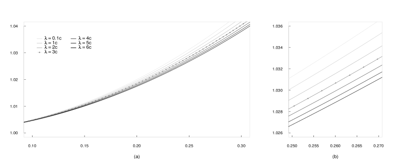
Figure 3: In (a) and (b) the mean-value E { cosh η c m ( t ) } 𝐸 subscript 𝜂 𝑐 𝑚 𝑡 E\{\cosh\eta_{cm}(t)\} c = 1 𝑐 1 c=1 λ 𝜆 \lambda λ = 3 c 𝜆 3 𝑐 \lambda=3c E { cosh η c m ( t ) } = e − c t ( 53 2 2 5 2 + 3 10 c t ) + e c t 5 2 2 3 + e − 7 c t 2 2 2 5 2 3 𝐸 subscript 𝜂 𝑐 𝑚 𝑡 superscript 𝑒 𝑐 𝑡 53 superscript 2 2 superscript 5 2 3 10 𝑐 𝑡 superscript 𝑒 𝑐 𝑡 5 superscript 2 2 3 superscript 𝑒 7 𝑐 𝑡 2 superscript 2 2 superscript 5 2 3 E\{\cosh\eta_{cm}(t)\}=e^{-ct}\left(\frac{53}{2^{2}5^{2}}+\frac{3}{10}ct\right)+e^{ct}\frac{5}{2^{2}3}+e^{-\frac{7ct}{2}}\frac{2^{2}}{5^{2}3}
In Figure 3 E { cosh η c m ( t ) } 𝐸 subscript 𝜂 𝑐 𝑚 𝑡 E\{\cosh\eta_{cm}(t)\} c = 1 𝑐 1 c=1 λ 𝜆 \lambda λ = 3 c 𝜆 3 𝑐 \lambda=3c λ = 3 c 𝜆 3 𝑐 \lambda=3c
Remark 4.2 .
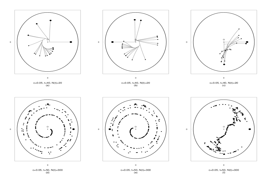
We now show that the center of mass (as well as each individual particle) goes further and further away from the origin O 𝑂 O H 2 + superscript subscript 𝐻 2 H_{2}^{+} D 𝐷 D t 𝑡 t 4.10
d d t E { cosh η c m ( t ) } d d 𝑡 𝐸 subscript 𝜂 𝑐 𝑚 𝑡 \displaystyle\frac{\mathrm{d}}{\mathrm{d}t}E\{\cosh\eta_{cm}(t)\} = \displaystyle= 2 2 c 2 e − 3 2 2 λ t λ 2 + 2 4 c 2 sinh t 2 2 λ 2 + 2 4 c 2 superscript 2 2 superscript 𝑐 2 superscript 𝑒 3 superscript 2 2 𝜆 𝑡 superscript 𝜆 2 superscript 2 4 superscript 𝑐 2 𝑡 superscript 2 2 superscript 𝜆 2 superscript 2 4 superscript 𝑐 2 \displaystyle\frac{2^{2}c^{2}e^{-\frac{3}{2^{2}}\lambda t}}{\sqrt{\lambda^{2}+2^{4}c^{2}}}\sinh\frac{t}{2^{2}}\sqrt{\lambda^{2}+2^{4}c^{2}} (4.15)
+ 2 c λ 2 λ 2 + 2 4 c 2 ∫ 0 t e − 3 2 2 λ s sinh c ( t − s ) sinh s 2 2 λ 2 + 2 4 c 2 d s 2 𝑐 superscript 𝜆 2 superscript 𝜆 2 superscript 2 4 superscript 𝑐 2 superscript subscript 0 𝑡 superscript 𝑒 3 superscript 2 2 𝜆 𝑠 𝑐 𝑡 𝑠 𝑠 superscript 2 2 superscript 𝜆 2 superscript 2 4 superscript 𝑐 2 d 𝑠 \displaystyle+\frac{2c\lambda^{2}}{\sqrt{\lambda^{2}+2^{4}c^{2}}}\int_{0}^{t}e^{-\frac{3}{2^{2}}\lambda s}\sinh c(t-s)\sinh\frac{s}{2^{2}}\sqrt{\lambda^{2}+2^{4}c^{2}}\mathrm{d}s
+ 2 2 c 2 λ λ 2 + 2 4 c 2 ∫ 0 t e − 3 2 2 λ s cosh c ( t − s ) sinh s 2 2 λ 2 + 2 4 c 2 d s . superscript 2 2 superscript 𝑐 2 𝜆 superscript 𝜆 2 superscript 2 4 superscript 𝑐 2 superscript subscript 0 𝑡 superscript 𝑒 3 superscript 2 2 𝜆 𝑠 𝑐 𝑡 𝑠 𝑠 superscript 2 2 superscript 𝜆 2 superscript 2 4 superscript 𝑐 2 d 𝑠 \displaystyle+\frac{2^{2}c^{2}\lambda}{\sqrt{\lambda^{2}+2^{4}c^{2}}}\int_{0}^{t}e^{-\frac{3}{2^{2}}\lambda s}\cosh c(t-s)\sinh\frac{s}{2^{2}}\sqrt{\lambda^{2}+2^{4}c^{2}}\mathrm{d}s.
The first term in the right hand side of (4.15 4.10 4.15 d 2 d t 2 E { cosh η c m ( t ) } > 0 superscript d 2 d superscript 𝑡 2 𝐸 subscript 𝜂 𝑐 𝑚 𝑡 0 \frac{\mathrm{d^{2}}}{\mathrm{d}t^{2}}E\{\cosh\eta_{cm}(t)\}>0 t 𝑡 t
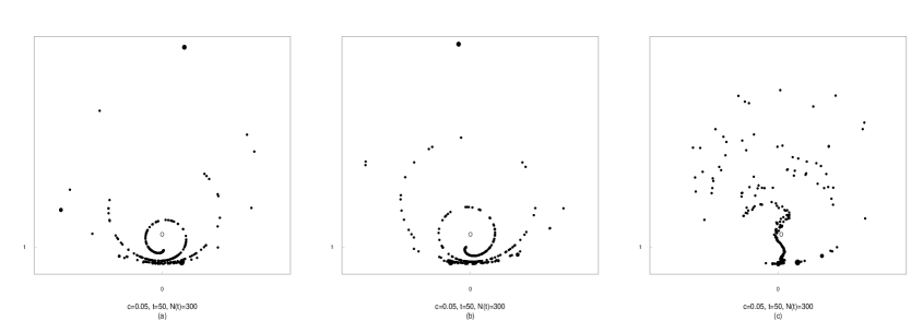
Figure 4: In (a), (b), and (c) the trajectories and the positions of the splinters at time t = 40 𝑡 40 t=40 c = 0.05 𝑐 0.05 c=0.05 N ( t ) = 20 𝑁 𝑡 20 N(t)=20 t = 50 𝑡 50 t=50 c = 0.05 𝑐 0.05 c=0.05 N ( t ) = 300 𝑁 𝑡 300 N(t)=300
5 Equation governing the hyperbolic distance
We are able to confirm result (4.1
E { cosh η c m ( t ) } = e − λ t ∑ n = 1 ∞ λ n ∑ k = 0 n − 1 1 2 k + 1 G n , k ( t ) + e − λ t ∑ n = 0 ∞ λ n 2 n G n , n ( t ) . 𝐸 subscript 𝜂 𝑐 𝑚 𝑡 superscript 𝑒 𝜆 𝑡 superscript subscript 𝑛 1 superscript 𝜆 𝑛 superscript subscript 𝑘 0 𝑛 1 1 superscript 2 𝑘 1 subscript 𝐺 𝑛 𝑘
𝑡 superscript 𝑒 𝜆 𝑡 superscript subscript 𝑛 0 superscript 𝜆 𝑛 superscript 2 𝑛 subscript 𝐺 𝑛 𝑛
𝑡 E\{\cosh\eta_{cm}(t)\}=e^{-\lambda t}\sum_{n=1}^{\infty}\lambda^{n}\sum_{k=0}^{n-1}\frac{1}{2^{k+1}}G_{n,k}(t)+e^{-\lambda t}\sum_{n=0}^{\infty}\frac{\lambda^{n}}{2^{n}}G_{n,n}(t). (5.1)
We start by deriving the difference-differential equations governing the functions G n , k ( t ) subscript 𝐺 𝑛 𝑘
𝑡 G_{n,k}(t) t > 0 𝑡 0 t>0 0 ≤ k ≤ n 0 𝑘 𝑛 0\leq k\leq n [1 ] , the j 𝑗 j j + 1 𝑗 1 j+1
Lemma 5.1 .
The functions represented by the following multiple integrals
G n , k ( t ) = ∫ 0 t d s 1 ⋯ ∫ s k − 1 t d s k ( t − s k ) ( n − k ) ! n − k ∏ j = 1 k cosh c ( s j − s j − 1 ) cosh c ( t − s k ) , 0 ≤ k ≤ n , formulae-sequence subscript 𝐺 𝑛 𝑘
𝑡 superscript subscript 0 𝑡 differential-d subscript 𝑠 1 ⋯ superscript subscript subscript 𝑠 𝑘 1 𝑡 differential-d subscript 𝑠 𝑘 superscript 𝑡 subscript 𝑠 𝑘 𝑛 𝑘 𝑛 𝑘 superscript subscript product 𝑗 1 𝑘 𝑐 subscript 𝑠 𝑗 subscript 𝑠 𝑗 1 𝑐 𝑡 subscript 𝑠 𝑘 0 𝑘 𝑛 G_{n,k}(t)=\int_{0}^{t}\mathrm{d}s_{1}\cdots\int_{s_{k-1}}^{t}\mathrm{d}s_{k}\;\frac{(t-s_{k})}{(n-k)!}^{n-k}\prod_{j=1}^{k}\cosh c(s_{j}-s_{j-1})\cosh c(t-s_{k}),\hskip 28.45274pt0\leq k\leq n,
are solutions to the difference-differential equations
{ d 2 d t 2 G n , k = 2 d d t G n − 1 , k − G n − 2 , k + c 2 G n , k , k ≤ n − 2 , d 2 d t 2 G n , n − 1 = 2 d d t G n − 1 , n − 1 − G n − 2 , n − 2 + c 2 G n , n − 1 , k = n − 1 , d 2 d t 2 G n , n = d d t G n − 1 , n − 1 + c 2 G n , n , k = n . cases superscript d 2 d superscript 𝑡 2 subscript 𝐺 𝑛 𝑘
2 d d 𝑡 subscript 𝐺 𝑛 1 𝑘
subscript 𝐺 𝑛 2 𝑘
superscript 𝑐 2 subscript 𝐺 𝑛 𝑘
𝑘 𝑛 2 superscript d 2 d superscript 𝑡 2 subscript 𝐺 𝑛 𝑛 1
2 d d 𝑡 subscript 𝐺 𝑛 1 𝑛 1
subscript 𝐺 𝑛 2 𝑛 2
superscript 𝑐 2 subscript 𝐺 𝑛 𝑛 1
𝑘 𝑛 1 superscript d 2 d superscript 𝑡 2 subscript 𝐺 𝑛 𝑛
d d 𝑡 subscript 𝐺 𝑛 1 𝑛 1
superscript 𝑐 2 subscript 𝐺 𝑛 𝑛
𝑘 𝑛 \left\{\begin{array}[]{lr}\frac{\mathrm{d}^{2}}{\mathrm{d}t^{2}}G_{n,k}=2\frac{\mathrm{d}}{\mathrm{d}t}G_{n-1,k}-G_{n-2,k}+c^{2}G_{n,k},&k\leq n-2,\\
\frac{\mathrm{d}^{2}}{\mathrm{d}t^{2}}G_{n,n-1}=2\frac{\mathrm{d}}{\mathrm{d}t}G_{n-1,n-1}-G_{n-2,n-2}+c^{2}G_{n,n-1},&k=n-1,\\
\frac{\mathrm{d}^{2}}{\mathrm{d}t^{2}}G_{n,n}=\frac{\mathrm{d}}{\mathrm{d}t}G_{n-1,n-1}+c^{2}G_{n,n},&k=n.\end{array}\right. (5.2)
Proof
We start by considering the case k ≤ n − 2 𝑘 𝑛 2 k\leq n-2
d d t G n , k d d 𝑡 subscript 𝐺 𝑛 𝑘
\displaystyle\frac{\mathrm{d}}{\mathrm{d}t}G_{n,k} = \displaystyle= G n − 1 , k + c ∫ 0 t d s 1 ⋯ ∫ s k − 1 t d s k ( t − s k ) n − k ( n − k ) ! ∏ j = 1 k cosh c ( s j − s j − 1 ) sinh c ( t − s k ) , subscript 𝐺 𝑛 1 𝑘
𝑐 superscript subscript 0 𝑡 differential-d subscript 𝑠 1 ⋯ superscript subscript subscript 𝑠 𝑘 1 𝑡 differential-d subscript 𝑠 𝑘 superscript 𝑡 subscript 𝑠 𝑘 𝑛 𝑘 𝑛 𝑘 superscript subscript product 𝑗 1 𝑘 𝑐 subscript 𝑠 𝑗 subscript 𝑠 𝑗 1 𝑐 𝑡 subscript 𝑠 𝑘 \displaystyle G_{n-1,k}+c\int_{0}^{t}\mathrm{d}s_{1}\cdots\int_{s_{k-1}}^{t}\mathrm{d}s_{k}\frac{(t-s_{k})^{n-k}}{(n-k)!}\prod_{j=1}^{k}\cosh c(s_{j}-s_{j-1})\sinh c(t-s_{k}), (5.3)
and, from (5.3
d 2 d t 2 G n , k superscript d 2 d superscript 𝑡 2 subscript 𝐺 𝑛 𝑘
\displaystyle\frac{\mathrm{d}^{2}}{\mathrm{d}t^{2}}G_{n,k} = \displaystyle= d d t G n − 1 , k + c 2 G n , k d d 𝑡 subscript 𝐺 𝑛 1 𝑘
superscript 𝑐 2 subscript 𝐺 𝑛 𝑘
\displaystyle\frac{\mathrm{d}}{\mathrm{d}t}G_{n-1,k}+c^{2}G_{n,k} (5.4)
+ c ∫ 0 t d s 1 ⋯ ∫ s k − 1 t d s k ( t − s k ) n − k − 1 ( n − k − 1 ) ! ∏ j = 1 k cosh c ( s j − s j − 1 ) sinh c ( t − s k ) 𝑐 superscript subscript 0 𝑡 differential-d subscript 𝑠 1 ⋯ superscript subscript subscript 𝑠 𝑘 1 𝑡 differential-d subscript 𝑠 𝑘 superscript 𝑡 subscript 𝑠 𝑘 𝑛 𝑘 1 𝑛 𝑘 1 superscript subscript product 𝑗 1 𝑘 𝑐 subscript 𝑠 𝑗 subscript 𝑠 𝑗 1 𝑐 𝑡 subscript 𝑠 𝑘 \displaystyle+c\int_{0}^{t}\mathrm{d}s_{1}\cdots\int_{s_{k-1}}^{t}\mathrm{d}s_{k}\frac{(t-s_{k})^{n-k-1}}{(n-k-1)!}\prod_{j=1}^{k}\cosh c(s_{j}-s_{j-1})\sinh c(t-s_{k})
= \displaystyle= 2 d d t G n − 1 , k − G n − 2 , k + c 2 G n , k . 2 d d 𝑡 subscript 𝐺 𝑛 1 𝑘
subscript 𝐺 𝑛 2 𝑘
superscript 𝑐 2 subscript 𝐺 𝑛 𝑘
\displaystyle 2\frac{\mathrm{d}}{\mathrm{d}t}G_{n-1,k}-G_{n-2,k}+c^{2}G_{n,k}.
The expression (5.3 k = n − 1 𝑘 𝑛 1 k=n-1
d d t G n , n − 1 d d 𝑡 subscript 𝐺 𝑛 𝑛 1
\displaystyle\frac{\mathrm{d}}{\mathrm{d}t}G_{n,n-1} = \displaystyle= G n − 1 , n − 1 subscript 𝐺 𝑛 1 𝑛 1
\displaystyle G_{n-1,n-1} (5.5)
+ c ∫ 0 t d s 1 ⋯ ∫ s n − 2 t d s n − 1 ( t − s n − 1 ) ∏ j = 1 n − 1 cosh c ( s j − s j − 1 ) sinh c ( t − s n − 1 ) , 𝑐 superscript subscript 0 𝑡 differential-d subscript 𝑠 1 ⋯ superscript subscript subscript 𝑠 𝑛 2 𝑡 differential-d subscript 𝑠 𝑛 1 𝑡 subscript 𝑠 𝑛 1 superscript subscript product 𝑗 1 𝑛 1 𝑐 subscript 𝑠 𝑗 subscript 𝑠 𝑗 1 𝑐 𝑡 subscript 𝑠 𝑛 1 \displaystyle+c\int_{0}^{t}\mathrm{d}s_{1}\cdots\int_{s_{n-2}}^{t}\mathrm{d}s_{n-1}(t-s_{n-1})\prod_{j=1}^{n-1}\cosh c(s_{j}-s_{j-1})\sinh c(t-s_{n-1}),
and thus, from (5.5
d 2 d t 2 G n , n − 1 superscript d 2 d superscript 𝑡 2 subscript 𝐺 𝑛 𝑛 1
\displaystyle\frac{\mathrm{d}^{2}}{\mathrm{d}t^{2}}G_{n,n-1} = \displaystyle= d d t G n − 1 , n − 1 + c 2 G n , n − 1 d d 𝑡 subscript 𝐺 𝑛 1 𝑛 1
superscript 𝑐 2 subscript 𝐺 𝑛 𝑛 1
\displaystyle\frac{\mathrm{d}}{\mathrm{d}t}G_{n-1,n-1}+c^{2}G_{n,n-1}
+ c ∫ 0 t d s 1 ⋯ ∫ s n − 2 t d s n − 1 ∏ j = 1 n − 1 cosh c ( s j − s j − 1 ) sinh c ( t − s n − 1 ) 𝑐 superscript subscript 0 𝑡 differential-d subscript 𝑠 1 ⋯ superscript subscript subscript 𝑠 𝑛 2 𝑡 differential-d subscript 𝑠 𝑛 1 superscript subscript product 𝑗 1 𝑛 1 𝑐 subscript 𝑠 𝑗 subscript 𝑠 𝑗 1 𝑐 𝑡 subscript 𝑠 𝑛 1 \displaystyle+c\int_{0}^{t}\mathrm{d}s_{1}\cdots\int_{s_{n-2}}^{t}\mathrm{d}s_{n-1}\prod_{j=1}^{n-1}\cosh c(s_{j}-s_{j-1})\sinh c(t-s_{n-1})
= \displaystyle= d d t G n − 1 , n − 1 + ( d d t G n − 1 , n − 1 − G n − 2 , n − 2 ) + c 2 G n , n − 1 d d 𝑡 subscript 𝐺 𝑛 1 𝑛 1
d d 𝑡 subscript 𝐺 𝑛 1 𝑛 1
subscript 𝐺 𝑛 2 𝑛 2
superscript 𝑐 2 subscript 𝐺 𝑛 𝑛 1
\displaystyle\frac{\mathrm{d}}{\mathrm{d}t}G_{n-1,n-1}+\left(\frac{\mathrm{d}}{\mathrm{d}t}G_{n-1,n-1}-G_{n-2,n-2}\right)+c^{2}G_{n,n-1}
= \displaystyle= 2 d d t G n − 1 , n − 1 − G n − 2 , n − 2 + c 2 G n , n − 1 . 2 d d 𝑡 subscript 𝐺 𝑛 1 𝑛 1
subscript 𝐺 𝑛 2 𝑛 2
superscript 𝑐 2 subscript 𝐺 𝑛 𝑛 1
\displaystyle 2\frac{\mathrm{d}}{\mathrm{d}t}G_{n-1,n-1}-G_{n-2,n-2}+c^{2}G_{n,n-1}.
We omit the derivation of the last formula in (5.2 [1 ] . ■ ■ \blacksquare
The results of Lemma 5.1
Theorem 5.1 .
The mean-value of (3.2 E { cosh η c m ( t ) } 𝐸 subscript 𝜂 𝑐 𝑚 𝑡 E\{\cosh\eta_{cm}(t)\}
d 2 d t 2 u − c 2 u = λ c 2 e − 3 2 2 λ t λ 2 + 2 4 c 2 { e − t 2 2 λ 2 + 2 4 c 2 − e t 2 2 λ 2 + 2 4 c 2 } . superscript d 2 d superscript 𝑡 2 𝑢 superscript 𝑐 2 𝑢 𝜆 superscript 𝑐 2 superscript 𝑒 3 superscript 2 2 𝜆 𝑡 superscript 𝜆 2 superscript 2 4 superscript 𝑐 2 superscript 𝑒 𝑡 superscript 2 2 superscript 𝜆 2 superscript 2 4 superscript 𝑐 2 superscript 𝑒 𝑡 superscript 2 2 superscript 𝜆 2 superscript 2 4 superscript 𝑐 2 \frac{\mathrm{d}^{2}}{\mathrm{d}t^{2}}u-c^{2}u=\frac{\lambda c^{2}e^{-\frac{3}{2^{2}}\lambda t}}{\sqrt{\lambda^{2}+2^{4}c^{2}}}\left\{e^{-\frac{t}{2^{2}}\sqrt{\lambda^{2}+2^{4}c^{2}}}-e^{\frac{t}{2^{2}}\sqrt{\lambda^{2}+2^{4}c^{2}}}\right\}. (5.6)
Proof
We begin by successively deriving the expression (5.1
d d t u = − λ u + e − λ t ∑ n = 1 ∞ λ n ∑ k = 0 n − 1 1 2 k + 1 d d t G n , k + e − λ t ∑ n = 0 ∞ λ n 2 n d d t G n , n , d d 𝑡 𝑢 𝜆 𝑢 superscript 𝑒 𝜆 𝑡 superscript subscript 𝑛 1 superscript 𝜆 𝑛 superscript subscript 𝑘 0 𝑛 1 1 superscript 2 𝑘 1 d d 𝑡 subscript 𝐺 𝑛 𝑘
superscript 𝑒 𝜆 𝑡 superscript subscript 𝑛 0 superscript 𝜆 𝑛 superscript 2 𝑛 d d 𝑡 subscript 𝐺 𝑛 𝑛
\frac{\mathrm{d}}{\mathrm{d}t}u=-\lambda u+e^{-\lambda t}\sum_{n=1}^{\infty}\lambda^{n}\sum_{k=0}^{n-1}\frac{1}{2^{k+1}}\frac{\mathrm{d}}{\mathrm{d}t}G_{n,k}+e^{-\lambda t}\sum_{n=0}^{\infty}\frac{\lambda^{n}}{2^{n}}\frac{\mathrm{d}}{\mathrm{d}t}G_{n,n},
and
d 2 d t 2 u superscript d 2 d superscript 𝑡 2 𝑢 \displaystyle\frac{\mathrm{d}^{2}}{\mathrm{d}t^{2}}u = \displaystyle= − 2 λ d d t u − λ 2 u + e − λ t ∑ n = 1 ∞ λ n ∑ k = 0 n − 1 1 2 k + 1 d 2 d t 2 G n , k + e − λ t ∑ n = 0 ∞ λ n 2 n d 2 d t 2 G n , n . 2 𝜆 d d 𝑡 𝑢 superscript 𝜆 2 𝑢 superscript 𝑒 𝜆 𝑡 superscript subscript 𝑛 1 superscript 𝜆 𝑛 superscript subscript 𝑘 0 𝑛 1 1 superscript 2 𝑘 1 superscript d 2 d superscript 𝑡 2 subscript 𝐺 𝑛 𝑘
superscript 𝑒 𝜆 𝑡 superscript subscript 𝑛 0 superscript 𝜆 𝑛 superscript 2 𝑛 superscript d 2 d superscript 𝑡 2 subscript 𝐺 𝑛 𝑛
\displaystyle-2\lambda\frac{\mathrm{d}}{\mathrm{d}t}u-\lambda^{2}u+e^{-\lambda t}\sum_{n=1}^{\infty}\lambda^{n}\sum_{k=0}^{n-1}\frac{1}{2^{k+1}}\frac{\mathrm{d}^{2}}{\mathrm{d}t^{2}}G_{n,k}+e^{-\lambda t}\sum_{n=0}^{\infty}\frac{\lambda^{n}}{2^{n}}\frac{\mathrm{d}^{2}}{\mathrm{d}t^{2}}G_{n,n}. (5.7)
We must now insert all the expressions of Lemma 5.1 5.7 n 𝑛 n k 𝑘 k 5.7
∑ n = 1 ∞ λ n ∑ k = 0 n − 1 1 2 k + 1 d 2 d t 2 G n , k + ∑ n = 0 ∞ λ n 2 n d 2 d t 2 G n , n superscript subscript 𝑛 1 superscript 𝜆 𝑛 superscript subscript 𝑘 0 𝑛 1 1 superscript 2 𝑘 1 superscript d 2 d superscript 𝑡 2 subscript 𝐺 𝑛 𝑘
superscript subscript 𝑛 0 superscript 𝜆 𝑛 superscript 2 𝑛 superscript d 2 d superscript 𝑡 2 subscript 𝐺 𝑛 𝑛
\displaystyle\sum_{n=1}^{\infty}\lambda^{n}\sum_{k=0}^{n-1}\frac{1}{2^{k+1}}\frac{\mathrm{d}^{2}}{\mathrm{d}t^{2}}G_{n,k}+\sum_{n=0}^{\infty}\frac{\lambda^{n}}{2^{n}}\frac{\mathrm{d}^{2}}{\mathrm{d}t^{2}}G_{n,n} (5.8)
= \displaystyle= ∑ n = 2 ∞ λ n ∑ k = 0 n − 2 1 2 k + 1 d 2 d t 2 G n , k + ∑ n = 2 ∞ λ n 2 n d 2 d t 2 G n , n − 1 + λ 2 d 2 d t 2 G 1 , 0 superscript subscript 𝑛 2 superscript 𝜆 𝑛 superscript subscript 𝑘 0 𝑛 2 1 superscript 2 𝑘 1 superscript d 2 d superscript 𝑡 2 subscript 𝐺 𝑛 𝑘
superscript subscript 𝑛 2 superscript 𝜆 𝑛 superscript 2 𝑛 superscript d 2 d superscript 𝑡 2 subscript 𝐺 𝑛 𝑛 1
𝜆 2 superscript d 2 d superscript 𝑡 2 subscript 𝐺 1 0
\displaystyle\sum_{n=2}^{\infty}\lambda^{n}\sum_{k=0}^{n-2}\frac{1}{2^{k+1}}\frac{\mathrm{d}^{2}}{\mathrm{d}t^{2}}G_{n,k}+\sum_{n=2}^{\infty}\frac{\lambda^{n}}{2^{n}}\frac{\mathrm{d}^{2}}{\mathrm{d}t^{2}}G_{n,n-1}+\frac{\lambda}{2}\frac{\mathrm{d}^{2}}{\mathrm{d}t^{2}}G_{1,0}
+ ∑ n = 1 ∞ λ n 2 n d 2 d t 2 G n , n + d 2 d t 2 G 0 , 0 superscript subscript 𝑛 1 superscript 𝜆 𝑛 superscript 2 𝑛 superscript d 2 d superscript 𝑡 2 subscript 𝐺 𝑛 𝑛
superscript d 2 d superscript 𝑡 2 subscript 𝐺 0 0
\displaystyle+\sum_{n=1}^{\infty}\frac{\lambda^{n}}{2^{n}}\frac{\mathrm{d}^{2}}{\mathrm{d}t^{2}}G_{n,n}+\frac{\mathrm{d}^{2}}{\mathrm{d}t^{2}}G_{0,0}
= \displaystyle= ∑ n = 2 ∞ λ n ∑ k = 0 n − 2 1 2 k + 1 [ 2 d d t G n − 1 , k − G n − 2 , k + c 2 G n , k ] superscript subscript 𝑛 2 superscript 𝜆 𝑛 superscript subscript 𝑘 0 𝑛 2 1 superscript 2 𝑘 1 delimited-[] 2 d d 𝑡 subscript 𝐺 𝑛 1 𝑘
subscript 𝐺 𝑛 2 𝑘
superscript 𝑐 2 subscript 𝐺 𝑛 𝑘
\displaystyle\sum_{n=2}^{\infty}\lambda^{n}\sum_{k=0}^{n-2}\frac{1}{2^{k+1}}\left[2\frac{\mathrm{d}}{\mathrm{d}t}G_{n-1,k}-G_{n-2,k}+c^{2}G_{n,k}\right]
+ ∑ n = 2 ∞ λ n 2 n [ 2 d d t G n − 1 , n − 1 − G n − 2 , n − 2 + c 2 G n , n − 1 ] + λ d d t G 0 , 0 + λ 2 c 2 G 1 , 0 superscript subscript 𝑛 2 superscript 𝜆 𝑛 superscript 2 𝑛 delimited-[] 2 d d 𝑡 subscript 𝐺 𝑛 1 𝑛 1
subscript 𝐺 𝑛 2 𝑛 2
superscript 𝑐 2 subscript 𝐺 𝑛 𝑛 1
𝜆 d d 𝑡 subscript 𝐺 0 0
𝜆 2 superscript 𝑐 2 subscript 𝐺 1 0
\displaystyle+\sum_{n=2}^{\infty}\frac{\lambda^{n}}{2^{n}}\left[2\frac{\mathrm{d}}{\mathrm{d}t}G_{n-1,n-1}-G_{n-2,n-2}+c^{2}G_{n,n-1}\right]+\lambda\frac{\mathrm{d}}{\mathrm{d}t}G_{0,0}+\frac{\lambda}{2}c^{2}G_{1,0}
+ ∑ n = 1 ∞ λ n 2 n [ d d t G n − 1 , n − 1 + c 2 G n , n ] + c 2 G 0 , 0 . superscript subscript 𝑛 1 superscript 𝜆 𝑛 superscript 2 𝑛 delimited-[] d d 𝑡 subscript 𝐺 𝑛 1 𝑛 1
superscript 𝑐 2 subscript 𝐺 𝑛 𝑛
superscript 𝑐 2 subscript 𝐺 0 0
\displaystyle+\sum_{n=1}^{\infty}\frac{\lambda^{n}}{2^{n}}\left[\frac{\mathrm{d}}{\mathrm{d}t}G_{n-1,n-1}+c^{2}G_{n,n}\right]+c^{2}G_{0,0}.
By regrouping the above terms we notice that (5.8
c 2 [ ∑ n = 1 ∞ λ n ∑ k = 0 n − 1 1 2 k + 1 G n , k + ∑ n = 0 ∞ λ n 2 n G n , n ] + 2 λ d d t [ ∑ n = 1 ∞ λ n ∑ k = 0 n − 1 1 2 k + 1 G n , k + ∑ n = 0 ∞ λ n 2 n G n , n ] superscript 𝑐 2 delimited-[] superscript subscript 𝑛 1 superscript 𝜆 𝑛 superscript subscript 𝑘 0 𝑛 1 1 superscript 2 𝑘 1 subscript 𝐺 𝑛 𝑘
superscript subscript 𝑛 0 superscript 𝜆 𝑛 superscript 2 𝑛 subscript 𝐺 𝑛 𝑛
2 𝜆 d d 𝑡 delimited-[] superscript subscript 𝑛 1 superscript 𝜆 𝑛 superscript subscript 𝑘 0 𝑛 1 1 superscript 2 𝑘 1 subscript 𝐺 𝑛 𝑘
superscript subscript 𝑛 0 superscript 𝜆 𝑛 superscript 2 𝑛 subscript 𝐺 𝑛 𝑛
\displaystyle c^{2}\left[\sum_{n=1}^{\infty}\lambda^{n}\sum_{k=0}^{n-1}\frac{1}{2^{k+1}}G_{n,k}+\sum_{n=0}^{\infty}\frac{\lambda^{n}}{2^{n}}G_{n,n}\right]+2\lambda\frac{\mathrm{d}}{\mathrm{d}t}\left[\sum_{n=1}^{\infty}\lambda^{n}\sum_{k=0}^{n-1}\frac{1}{2^{k+1}}G_{n,k}+\sum_{n=0}^{\infty}\frac{\lambda^{n}}{2^{n}}G_{n,n}\right] (5.9)
− λ 2 [ ∑ n = 1 ∞ λ n ∑ k = 0 n − 1 1 2 k + 1 G n , k + ∑ n = 0 ∞ λ n 2 n G n , n ] − λ 2 ∑ n = 0 ∞ λ n 2 n d d t G n , n + λ 2 2 2 ∑ n = 0 ∞ λ n 2 n G n , n superscript 𝜆 2 delimited-[] superscript subscript 𝑛 1 superscript 𝜆 𝑛 superscript subscript 𝑘 0 𝑛 1 1 superscript 2 𝑘 1 subscript 𝐺 𝑛 𝑘
superscript subscript 𝑛 0 superscript 𝜆 𝑛 superscript 2 𝑛 subscript 𝐺 𝑛 𝑛
𝜆 2 superscript subscript 𝑛 0 superscript 𝜆 𝑛 superscript 2 𝑛 d d 𝑡 subscript 𝐺 𝑛 𝑛
superscript 𝜆 2 superscript 2 2 superscript subscript 𝑛 0 superscript 𝜆 𝑛 superscript 2 𝑛 subscript 𝐺 𝑛 𝑛
\displaystyle-\lambda^{2}\left[\sum_{n=1}^{\infty}\lambda^{n}\sum_{k=0}^{n-1}\frac{1}{2^{k+1}}G_{n,k}+\sum_{n=0}^{\infty}\frac{\lambda^{n}}{2^{n}}G_{n,n}\right]-\frac{\lambda}{2}\sum_{n=0}^{\infty}\frac{\lambda^{n}}{2^{n}}\frac{\mathrm{d}}{\mathrm{d}t}G_{n,n}+\frac{\lambda^{2}}{2^{2}}\sum_{n=0}^{\infty}\frac{\lambda^{n}}{2^{n}}G_{n,n}
= \displaystyle= c 2 e λ t u + 2 λ d d t [ e λ t u ] − λ 2 e λ t u − λ 2 ∑ n = 0 ∞ λ n 2 n d d t G n , n + λ 2 2 2 ∑ n = 0 ∞ λ n 2 n G n , n . superscript 𝑐 2 superscript 𝑒 𝜆 𝑡 𝑢 2 𝜆 d d 𝑡 delimited-[] superscript 𝑒 𝜆 𝑡 𝑢 superscript 𝜆 2 superscript 𝑒 𝜆 𝑡 𝑢 𝜆 2 superscript subscript 𝑛 0 superscript 𝜆 𝑛 superscript 2 𝑛 d d 𝑡 subscript 𝐺 𝑛 𝑛
superscript 𝜆 2 superscript 2 2 superscript subscript 𝑛 0 superscript 𝜆 𝑛 superscript 2 𝑛 subscript 𝐺 𝑛 𝑛
\displaystyle c^{2}e^{\lambda t}u+2\lambda\frac{\mathrm{d}}{\mathrm{d}t}[e^{\lambda t}u]-\lambda^{2}e^{\lambda t}u-\frac{\lambda}{2}\sum_{n=0}^{\infty}\frac{\lambda^{n}}{2^{n}}\frac{\mathrm{d}}{\mathrm{d}t}G_{n,n}+\frac{\lambda^{2}}{2^{2}}\sum_{n=0}^{\infty}\frac{\lambda^{n}}{2^{n}}G_{n,n}.
Multiplying by e − λ t superscript 𝑒 𝜆 𝑡 e^{-\lambda t} 5.9
e − λ t ∑ n = 1 ∞ λ n ∑ k = 0 n − 1 1 2 k + 1 d 2 d t 2 G n , k + e − λ t ∑ n = 0 ∞ λ n 2 n d 2 d t 2 G n , n superscript 𝑒 𝜆 𝑡 superscript subscript 𝑛 1 superscript 𝜆 𝑛 superscript subscript 𝑘 0 𝑛 1 1 superscript 2 𝑘 1 superscript d 2 d superscript 𝑡 2 subscript 𝐺 𝑛 𝑘
superscript 𝑒 𝜆 𝑡 superscript subscript 𝑛 0 superscript 𝜆 𝑛 superscript 2 𝑛 superscript d 2 d superscript 𝑡 2 subscript 𝐺 𝑛 𝑛
\displaystyle e^{-\lambda t}\sum_{n=1}^{\infty}\lambda^{n}\sum_{k=0}^{n-1}\frac{1}{2^{k+1}}\frac{\mathrm{d}^{2}}{\mathrm{d}t^{2}}G_{n,k}+e^{-\lambda t}\sum_{n=0}^{\infty}\frac{\lambda^{n}}{2^{n}}\frac{\mathrm{d}^{2}}{\mathrm{d}t^{2}}G_{n,n} (5.10)
= \displaystyle= c 2 u + 2 λ 2 u + 2 λ d d t u − λ 2 u − λ 2 e − λ t ∑ n = 0 ∞ λ n 2 n d d t G n , n + λ 2 2 2 e − λ t ∑ n = 0 ∞ λ n 2 n G n , n . superscript 𝑐 2 𝑢 2 superscript 𝜆 2 𝑢 2 𝜆 d d 𝑡 𝑢 superscript 𝜆 2 𝑢 𝜆 2 superscript 𝑒 𝜆 𝑡 superscript subscript 𝑛 0 superscript 𝜆 𝑛 superscript 2 𝑛 d d 𝑡 subscript 𝐺 𝑛 𝑛
superscript 𝜆 2 superscript 2 2 superscript 𝑒 𝜆 𝑡 superscript subscript 𝑛 0 superscript 𝜆 𝑛 superscript 2 𝑛 subscript 𝐺 𝑛 𝑛
\displaystyle c^{2}u+2\lambda^{2}u+2\lambda\frac{\mathrm{d}}{\mathrm{d}t}u-\lambda^{2}u-\frac{\lambda}{2}e^{-\lambda t}\sum_{n=0}^{\infty}\frac{\lambda^{n}}{2^{n}}\frac{\mathrm{d}}{\mathrm{d}t}G_{n,n}+\frac{\lambda^{2}}{2^{2}}e^{-\lambda t}\sum_{n=0}^{\infty}\frac{\lambda^{n}}{2^{n}}G_{n,n}.
By inserting result (5.10 5.7
d 2 d t 2 u − c 2 u superscript d 2 d superscript 𝑡 2 𝑢 superscript 𝑐 2 𝑢 \displaystyle\frac{\mathrm{d}^{2}}{\mathrm{d}t^{2}}u-c^{2}u = \displaystyle= − λ 2 e − λ t ∑ n = 0 ∞ λ n 2 n d d t G n , n + λ 2 2 2 e − λ t ∑ n = 0 ∞ λ n 2 n G n , n . 𝜆 2 superscript 𝑒 𝜆 𝑡 superscript subscript 𝑛 0 superscript 𝜆 𝑛 superscript 2 𝑛 d d 𝑡 subscript 𝐺 𝑛 𝑛
superscript 𝜆 2 superscript 2 2 superscript 𝑒 𝜆 𝑡 superscript subscript 𝑛 0 superscript 𝜆 𝑛 superscript 2 𝑛 subscript 𝐺 𝑛 𝑛
\displaystyle-\frac{\lambda}{2}e^{-\lambda t}\sum_{n=0}^{\infty}\frac{\lambda^{n}}{2^{n}}\frac{\mathrm{d}}{\mathrm{d}t}G_{n,n}+\frac{\lambda^{2}}{2^{2}}e^{-\lambda t}\sum_{n=0}^{\infty}\frac{\lambda^{n}}{2^{n}}G_{n,n}. (5.11)
The series e − λ t 2 ∑ n = 0 ∞ λ n 2 n G n , n superscript 𝑒 𝜆 𝑡 2 superscript subscript 𝑛 0 superscript 𝜆 𝑛 superscript 2 𝑛 subscript 𝐺 𝑛 𝑛
e^{-\frac{\lambda t}{2}}\sum_{n=0}^{\infty}\frac{\lambda^{n}}{2^{n}}G_{n,n} [1 ] and represents the mean hyperbolic distance of the particle moving in H 2 + superscript subscript 𝐻 2 H_{2}^{+} λ / 2 𝜆 2 \lambda/2
e − λ t 2 ∑ n = 0 ∞ λ n 2 n G n , n = e − λ t 4 2 [ ( 1 + λ λ 2 + 2 4 c 2 ) e t 4 λ 2 + 2 4 c 2 + ( 1 − λ λ 2 + 2 4 c 2 ) e − t 4 λ 2 + 2 4 c 2 ] . superscript 𝑒 𝜆 𝑡 2 superscript subscript 𝑛 0 superscript 𝜆 𝑛 superscript 2 𝑛 subscript 𝐺 𝑛 𝑛
superscript 𝑒 𝜆 𝑡 4 2 delimited-[] 1 𝜆 superscript 𝜆 2 superscript 2 4 superscript 𝑐 2 superscript 𝑒 𝑡 4 superscript 𝜆 2 superscript 2 4 superscript 𝑐 2 1 𝜆 superscript 𝜆 2 superscript 2 4 superscript 𝑐 2 superscript 𝑒 𝑡 4 superscript 𝜆 2 superscript 2 4 superscript 𝑐 2 e^{-\frac{\lambda t}{2}}\sum_{n=0}^{\infty}\frac{\lambda^{n}}{2^{n}}G_{n,n}=\frac{e^{-\frac{\lambda t}{4}}}{2}\left[\left(1+\frac{\lambda}{\sqrt{\lambda^{2}+2^{4}c^{2}}}\right)e^{\frac{t}{4}\sqrt{\lambda^{2}+2^{4}c^{2}}}+\left(1-\frac{\lambda}{\sqrt{\lambda^{2}+2^{4}c^{2}}}\right)e^{-\frac{t}{4}\sqrt{\lambda^{2}+2^{4}c^{2}}}\right].
Since
e − λ t 2 ∑ n = 0 ∞ λ n 2 n d d t G n , n = d d t [ e − λ t 2 ∑ n = 0 ∞ λ n 2 n G n , n ] + λ 2 e − λ t 2 ∑ n = 0 ∞ λ n 2 n G n , n , superscript 𝑒 𝜆 𝑡 2 superscript subscript 𝑛 0 superscript 𝜆 𝑛 superscript 2 𝑛 d d 𝑡 subscript 𝐺 𝑛 𝑛
d d 𝑡 delimited-[] superscript 𝑒 𝜆 𝑡 2 superscript subscript 𝑛 0 superscript 𝜆 𝑛 superscript 2 𝑛 subscript 𝐺 𝑛 𝑛
𝜆 2 superscript 𝑒 𝜆 𝑡 2 superscript subscript 𝑛 0 superscript 𝜆 𝑛 superscript 2 𝑛 subscript 𝐺 𝑛 𝑛
e^{-\frac{\lambda t}{2}}\sum_{n=0}^{\infty}\frac{\lambda^{n}}{2^{n}}\frac{\mathrm{d}}{\mathrm{d}t}G_{n,n}=\frac{\mathrm{d}}{\mathrm{d}t}\left[e^{-\frac{\lambda t}{2}}\sum_{n=0}^{\infty}\frac{\lambda^{n}}{2^{n}}G_{n,n}\right]+\frac{\lambda}{2}e^{-\frac{\lambda t}{2}}\sum_{n=0}^{\infty}\frac{\lambda^{n}}{2^{n}}G_{n,n},
the right-hand side of (5.11
− λ 2 e − λ t ∑ n = 0 ∞ λ n 2 n d d t G n , n + λ 2 2 2 e − λ t ∑ n = 0 ∞ λ n 2 n G n , n = − λ 2 e − λ t 2 d d t [ e − λ t 2 ∑ n = 0 ∞ λ n 2 n G n , n ] 𝜆 2 superscript 𝑒 𝜆 𝑡 superscript subscript 𝑛 0 superscript 𝜆 𝑛 superscript 2 𝑛 d d 𝑡 subscript 𝐺 𝑛 𝑛
superscript 𝜆 2 superscript 2 2 superscript 𝑒 𝜆 𝑡 superscript subscript 𝑛 0 superscript 𝜆 𝑛 superscript 2 𝑛 subscript 𝐺 𝑛 𝑛
𝜆 2 superscript 𝑒 𝜆 𝑡 2 d d 𝑡 delimited-[] superscript 𝑒 𝜆 𝑡 2 superscript subscript 𝑛 0 superscript 𝜆 𝑛 superscript 2 𝑛 subscript 𝐺 𝑛 𝑛
\displaystyle-\frac{\lambda}{2}e^{-\lambda t}\sum_{n=0}^{\infty}\frac{\lambda^{n}}{2^{n}}\frac{\mathrm{d}}{\mathrm{d}t}G_{n,n}+\frac{\lambda^{2}}{2^{2}}e^{-\lambda t}\sum_{n=0}^{\infty}\frac{\lambda^{n}}{2^{n}}G_{n,n}=-\frac{\lambda}{2}e^{-\frac{\lambda t}{2}}\frac{\mathrm{d}}{\mathrm{d}t}\left[e^{-\frac{\lambda t}{2}}\sum_{n=0}^{\infty}\frac{\lambda^{n}}{2^{n}}G_{n,n}\right]
= \displaystyle= − λ 2 e − λ t 2 { − λ 2 3 e − λ t 2 2 [ ( 1 + λ λ 2 + 2 4 c 2 ) e t 2 2 λ 2 + 2 4 c 2 + ( 1 − λ λ 2 + 2 4 c 2 ) e − t 2 2 λ 2 + 2 4 c 2 ] \displaystyle-\frac{\lambda}{2}e^{-\frac{\lambda t}{2}}\left\{-\frac{\lambda}{2^{3}}e^{-\frac{\lambda t}{2^{2}}}\left[\left(1+\frac{\lambda}{\sqrt{\lambda^{2}+2^{4}c^{2}}}\right)e^{\frac{t}{2^{2}}\sqrt{\lambda^{2}+2^{4}c^{2}}}+\left(1-\frac{\lambda}{\sqrt{\lambda^{2}+2^{4}c^{2}}}\right)e^{-\frac{t}{2^{2}}\sqrt{\lambda^{2}+2^{4}c^{2}}}\right]\right.
+ λ 2 + 2 4 c 2 2 3 e − λ t 2 2 [ ( 1 + λ λ 2 + 2 4 c 2 ) e t 2 2 λ 2 + 2 4 c 2 − ( 1 − λ λ 2 + 2 4 c 2 ) e − t 2 2 λ 2 + 2 4 c 2 ] } \displaystyle+\left.\frac{\sqrt{\lambda^{2}+2^{4}c^{2}}}{2^{3}}e^{-\frac{\lambda t}{2^{2}}}\left[\left(1+\frac{\lambda}{\sqrt{\lambda^{2}+2^{4}c^{2}}}\right)e^{\frac{t}{2^{2}}\sqrt{\lambda^{2}+2^{4}c^{2}}}-\left(1-\frac{\lambda}{\sqrt{\lambda^{2}+2^{4}c^{2}}}\right)e^{-\frac{t}{2^{2}}\sqrt{\lambda^{2}+2^{4}c^{2}}}\right]\right\}
= \displaystyle= λ 2 2 4 e − 3 λ t 2 2 [ ( 1 + λ λ 2 + 2 4 c 2 ) e t 2 2 λ 2 + 2 4 c 2 + ( 1 − λ λ 2 + 2 4 c 2 ) e − t 2 2 λ 2 + 2 4 c 2 ] superscript 𝜆 2 superscript 2 4 superscript 𝑒 3 𝜆 𝑡 superscript 2 2 delimited-[] 1 𝜆 superscript 𝜆 2 superscript 2 4 superscript 𝑐 2 superscript 𝑒 𝑡 superscript 2 2 superscript 𝜆 2 superscript 2 4 superscript 𝑐 2 1 𝜆 superscript 𝜆 2 superscript 2 4 superscript 𝑐 2 superscript 𝑒 𝑡 superscript 2 2 superscript 𝜆 2 superscript 2 4 superscript 𝑐 2 \displaystyle\frac{\lambda^{2}}{2^{4}}e^{-\frac{3\lambda t}{2^{2}}}\left[\left(1+\frac{\lambda}{\sqrt{\lambda^{2}+2^{4}c^{2}}}\right)e^{\frac{t}{2^{2}}\sqrt{\lambda^{2}+2^{4}c^{2}}}+\left(1-\frac{\lambda}{\sqrt{\lambda^{2}+2^{4}c^{2}}}\right)e^{-\frac{t}{2^{2}}\sqrt{\lambda^{2}+2^{4}c^{2}}}\right]
− λ λ 2 + 2 4 c 2 2 4 e − 3 λ t 2 2 [ ( 1 + λ λ 2 + 2 4 c 2 ) e t 2 2 λ 2 + 2 4 c 2 − ( 1 − λ λ 2 + 2 4 c 2 ) e − t 2 2 λ 2 + 2 4 c 2 ] 𝜆 superscript 𝜆 2 superscript 2 4 superscript 𝑐 2 superscript 2 4 superscript 𝑒 3 𝜆 𝑡 superscript 2 2 delimited-[] 1 𝜆 superscript 𝜆 2 superscript 2 4 superscript 𝑐 2 superscript 𝑒 𝑡 superscript 2 2 superscript 𝜆 2 superscript 2 4 superscript 𝑐 2 1 𝜆 superscript 𝜆 2 superscript 2 4 superscript 𝑐 2 superscript 𝑒 𝑡 superscript 2 2 superscript 𝜆 2 superscript 2 4 superscript 𝑐 2 \displaystyle-\frac{\lambda\sqrt{\lambda^{2}+2^{4}c^{2}}}{2^{4}}e^{-\frac{3\lambda t}{2^{2}}}\left[\left(1+\frac{\lambda}{\sqrt{\lambda^{2}+2^{4}c^{2}}}\right)e^{\frac{t}{2^{2}}\sqrt{\lambda^{2}+2^{4}c^{2}}}-\left(1-\frac{\lambda}{\sqrt{\lambda^{2}+2^{4}c^{2}}}\right)e^{-\frac{t}{2^{2}}\sqrt{\lambda^{2}+2^{4}c^{2}}}\right]
= \displaystyle= − e − 3 λ t 2 2 e t 2 2 λ 2 + 2 4 c 2 λ c 2 λ 2 + 2 4 c 2 + e − 3 λ t 2 2 e − t 2 2 λ 2 + 2 4 c 2 λ c 2 λ 2 + 2 4 c 2 . superscript 𝑒 3 𝜆 𝑡 superscript 2 2 superscript 𝑒 𝑡 superscript 2 2 superscript 𝜆 2 superscript 2 4 superscript 𝑐 2 𝜆 superscript 𝑐 2 superscript 𝜆 2 superscript 2 4 superscript 𝑐 2 superscript 𝑒 3 𝜆 𝑡 superscript 2 2 superscript 𝑒 𝑡 superscript 2 2 superscript 𝜆 2 superscript 2 4 superscript 𝑐 2 𝜆 superscript 𝑐 2 superscript 𝜆 2 superscript 2 4 superscript 𝑐 2 \displaystyle-e^{-\frac{3\lambda t}{2^{2}}}e^{\frac{t}{2^{2}}\sqrt{\lambda^{2}+2^{4}c^{2}}}\frac{\lambda c^{2}}{\sqrt{\lambda^{2}+2^{4}c^{2}}}+e^{-\frac{3\lambda t}{2^{2}}}e^{-\frac{t}{2^{2}}\sqrt{\lambda^{2}+2^{4}c^{2}}}\frac{\lambda c^{2}}{\sqrt{\lambda^{2}+2^{4}c^{2}}}.
This lets equation (5.6 ■ ■ \blacksquare
The expression (4.1 E { cosh η c m ( t ) } 𝐸 subscript 𝜂 𝑐 𝑚 𝑡 E\{\cosh\eta_{cm}(t)\} 5.6 4.1
Theorem 5.2 .
The mean hyperbolic distance (4.1
{ d 2 d t 2 u − c 2 u = λ c 2 e − 3 2 2 λ t λ 2 + 2 4 c 2 { e − t 2 2 λ 2 + 2 4 c 2 − e t 2 2 λ 2 + 2 4 c 2 } , u ( 0 ) = 1 , d d t u ( t ) | t = 0 = 0 . cases superscript d 2 d superscript 𝑡 2 𝑢 superscript 𝑐 2 𝑢 𝜆 superscript 𝑐 2 superscript 𝑒 3 superscript 2 2 𝜆 𝑡 superscript 𝜆 2 superscript 2 4 superscript 𝑐 2 superscript 𝑒 𝑡 superscript 2 2 superscript 𝜆 2 superscript 2 4 superscript 𝑐 2 superscript 𝑒 𝑡 superscript 2 2 superscript 𝜆 2 superscript 2 4 superscript 𝑐 2 missing-subexpression 𝑢 0 1 missing-subexpression evaluated-at d d 𝑡 𝑢 𝑡 𝑡 0 0 missing-subexpression \left\{\begin{array}[]{lr}\frac{\mathrm{d}^{2}}{\mathrm{d}t^{2}}u-c^{2}u=\frac{\lambda c^{2}e^{-\frac{3}{2^{2}}\lambda t}}{\sqrt{\lambda^{2}+2^{4}c^{2}}}\left\{e^{-\frac{t}{2^{2}}\sqrt{\lambda^{2}+2^{4}c^{2}}}-e^{\frac{t}{2^{2}}\sqrt{\lambda^{2}+2^{4}c^{2}}}\right\},\\
u(0)=1,\\
\left.\frac{\mathrm{d}}{\mathrm{d}t}u(t)\right|_{t=0}=0.\end{array}\right.
Proof
In order to perform the calculations it is convenient to write (4.1
E { cosh η c m ( t ) } = K A ( t ) B ( t ) + λ + 2 c 2 ( λ + 3 c ) e c t + λ − 2 c 2 ( λ − 3 c ) e − c t 𝐸 subscript 𝜂 𝑐 𝑚 𝑡 𝐾 𝐴 𝑡 𝐵 𝑡 𝜆 2 𝑐 2 𝜆 3 𝑐 superscript 𝑒 𝑐 𝑡 𝜆 2 𝑐 2 𝜆 3 𝑐 superscript 𝑒 𝑐 𝑡 E\{\cosh\eta_{cm}(t)\}=KA(t)B(t)+\frac{\lambda+2c}{2(\lambda+3c)}e^{ct}+\frac{\lambda-2c}{2(\lambda-3c)}e^{-ct}
where
K = 2 3 c 2 λ 2 + 2 4 c 2 , A ( t ) = e − 3 2 2 λ t , B ( t ) = e − t 2 2 λ 2 + 2 4 c 2 5 λ + 3 λ 2 + 2 4 c 2 − e t 2 2 λ 2 + 2 4 c 2 5 λ − 3 λ 2 + 2 4 c 2 , formulae-sequence 𝐾 superscript 2 3 superscript 𝑐 2 superscript 𝜆 2 superscript 2 4 superscript 𝑐 2 formulae-sequence 𝐴 𝑡 superscript 𝑒 3 superscript 2 2 𝜆 𝑡 𝐵 𝑡 superscript 𝑒 𝑡 superscript 2 2 superscript 𝜆 2 superscript 2 4 superscript 𝑐 2 5 𝜆 3 superscript 𝜆 2 superscript 2 4 superscript 𝑐 2 superscript 𝑒 𝑡 superscript 2 2 superscript 𝜆 2 superscript 2 4 superscript 𝑐 2 5 𝜆 3 superscript 𝜆 2 superscript 2 4 superscript 𝑐 2 K=\frac{2^{3}c^{2}}{\sqrt{\lambda^{2}+2^{4}c^{2}}},\hskip 14.22636ptA(t)=e^{-\frac{3}{2^{2}}\lambda t},\hskip 14.22636ptB(t)=\frac{e^{-\frac{t}{2^{2}}\sqrt{\lambda^{2}+2^{4}c^{2}}}}{5\lambda+3\sqrt{\lambda^{2}+2^{4}c^{2}}}-\frac{e^{\frac{t}{2^{2}}\sqrt{\lambda^{2}+2^{4}c^{2}}}}{5\lambda-3\sqrt{\lambda^{2}+2^{4}c^{2}}},
and B ( t ) 𝐵 𝑡 B(t)
B ′ ( t ) = − λ 2 + 2 4 c 2 2 2 [ e − t 2 2 λ 2 + 2 4 c 2 5 λ + 3 λ 2 + 2 4 c 2 + e t 2 2 λ 2 + 2 4 c 2 5 λ − 3 λ 2 + 2 4 c 2 ] , B ′′ ( t ) = λ 2 + 2 4 c 2 2 4 B ( t ) . formulae-sequence superscript 𝐵 ′ 𝑡 superscript 𝜆 2 superscript 2 4 superscript 𝑐 2 superscript 2 2 delimited-[] superscript 𝑒 𝑡 superscript 2 2 superscript 𝜆 2 superscript 2 4 superscript 𝑐 2 5 𝜆 3 superscript 𝜆 2 superscript 2 4 superscript 𝑐 2 superscript 𝑒 𝑡 superscript 2 2 superscript 𝜆 2 superscript 2 4 superscript 𝑐 2 5 𝜆 3 superscript 𝜆 2 superscript 2 4 superscript 𝑐 2 superscript 𝐵 ′′ 𝑡 superscript 𝜆 2 superscript 2 4 superscript 𝑐 2 superscript 2 4 𝐵 𝑡 B^{\prime}(t)=-\frac{\sqrt{\lambda^{2}+2^{4}c^{2}}}{2^{2}}\left[\frac{e^{-\frac{t}{2^{2}}\sqrt{\lambda^{2}+2^{4}c^{2}}}}{5\lambda+3\sqrt{\lambda^{2}+2^{4}c^{2}}}+\frac{e^{\frac{t}{2^{2}}\sqrt{\lambda^{2}+2^{4}c^{2}}}}{5\lambda-3\sqrt{\lambda^{2}+2^{4}c^{2}}}\right],\hskip 14.22636ptB^{\prime\prime}(t)=\frac{\lambda^{2}+2^{4}c^{2}}{2^{4}}B(t).
Therefore
d 2 d t 2 E { cosh η c m ( t ) } − c 2 E { cosh η c m ( t ) } = λ K A 2 [ 5 λ 2 2 B − 3 B ′ ] superscript d 2 d superscript 𝑡 2 𝐸 subscript 𝜂 𝑐 𝑚 𝑡 superscript 𝑐 2 𝐸 subscript 𝜂 𝑐 𝑚 𝑡 𝜆 𝐾 𝐴 2 delimited-[] 5 𝜆 superscript 2 2 𝐵 3 superscript 𝐵 ′ \displaystyle\frac{\mathrm{d^{2}}}{\mathrm{d}t^{2}}E\{\cosh\eta_{cm}(t)\}-c^{2}E\{\cosh\eta_{cm}(t)\}=\frac{\lambda KA}{2}\left[\frac{5\lambda}{2^{2}}B-3B^{\prime}\right]
= \displaystyle= 2 2 λ c 2 e − 3 2 2 λ t λ 2 + 2 4 c 2 { 5 λ 2 2 [ e − t 2 2 λ 2 + 2 4 c 2 5 λ + 3 λ 2 + 2 4 c 2 − e t 2 2 λ 2 + 2 4 c 2 5 λ − 3 λ 2 + 2 4 c 2 ] \displaystyle\frac{2^{2}\lambda c^{2}e^{-\frac{3}{2^{2}}\lambda t}}{\sqrt{\lambda^{2}+2^{4}c^{2}}}\left\{\frac{5\lambda}{2^{2}}\left[\frac{e^{-\frac{t}{2^{2}}\sqrt{\lambda^{2}+2^{4}c^{2}}}}{5\lambda+3\sqrt{\lambda^{2}+2^{4}c^{2}}}-\frac{e^{\frac{t}{2^{2}}\sqrt{\lambda^{2}+2^{4}c^{2}}}}{5\lambda-3\sqrt{\lambda^{2}+2^{4}c^{2}}}\right]\right.
+ 3 λ 2 + 2 4 c 2 2 2 ( e − t 2 2 λ 2 + 2 4 c 2 5 λ + 3 λ 2 + 2 4 c 2 + e t 2 2 λ 2 + 2 4 c 2 5 λ − 3 λ 2 + 2 4 c 2 ) } \displaystyle+\left.3\;\frac{\sqrt{\lambda^{2}+2^{4}c^{2}}}{2^{2}}\left(\frac{e^{-\frac{t}{2^{2}}\sqrt{\lambda^{2}+2^{4}c^{2}}}}{5\lambda+3\sqrt{\lambda^{2}+2^{4}c^{2}}}+\frac{e^{\frac{t}{2^{2}}\sqrt{\lambda^{2}+2^{4}c^{2}}}}{5\lambda-3\sqrt{\lambda^{2}+2^{4}c^{2}}}\right)\right\}
= \displaystyle= λ c 2 e − 3 2 2 λ t λ 2 + 2 4 c 2 [ e − t 4 λ 2 + 2 4 c 2 5 λ + 3 λ 2 + 2 4 c 2 ( 5 λ + 3 λ 2 + 2 4 c 2 ) + e t 4 λ 2 + 2 4 c 2 5 λ − 3 λ 2 + 2 4 c 2 ( − 5 λ + 3 λ 2 + 2 4 c 2 ) ] 𝜆 superscript 𝑐 2 superscript 𝑒 3 superscript 2 2 𝜆 𝑡 superscript 𝜆 2 superscript 2 4 superscript 𝑐 2 delimited-[] superscript 𝑒 𝑡 4 superscript 𝜆 2 superscript 2 4 superscript 𝑐 2 5 𝜆 3 superscript 𝜆 2 superscript 2 4 superscript 𝑐 2 5 𝜆 3 superscript 𝜆 2 superscript 2 4 superscript 𝑐 2 superscript 𝑒 𝑡 4 superscript 𝜆 2 superscript 2 4 superscript 𝑐 2 5 𝜆 3 superscript 𝜆 2 superscript 2 4 superscript 𝑐 2 5 𝜆 3 superscript 𝜆 2 superscript 2 4 superscript 𝑐 2 \displaystyle\frac{\lambda c^{2}e^{-\frac{3}{2^{2}}\lambda t}}{\sqrt{\lambda^{2}+2^{4}c^{2}}}\left[\frac{e^{-\frac{t}{4}\sqrt{\lambda^{2}+2^{4}c^{2}}}}{5\lambda+3\sqrt{\lambda^{2}+2^{4}c^{2}}}(5\lambda+3\sqrt{\lambda^{2}+2^{4}c^{2}})+\frac{e^{\frac{t}{4}\sqrt{\lambda^{2}+2^{4}c^{2}}}}{5\lambda-3\sqrt{\lambda^{2}+2^{4}c^{2}}}(-5\lambda+3\sqrt{\lambda^{2}+2^{4}c^{2}})\right]
= \displaystyle= λ c 2 e − 3 2 2 λ t λ 2 + 2 4 c 2 [ e − t 4 λ 2 + 2 4 c 2 − e t 4 λ 2 + 2 4 c 2 ] . 𝜆 superscript 𝑐 2 superscript 𝑒 3 superscript 2 2 𝜆 𝑡 superscript 𝜆 2 superscript 2 4 superscript 𝑐 2 delimited-[] superscript 𝑒 𝑡 4 superscript 𝜆 2 superscript 2 4 superscript 𝑐 2 superscript 𝑒 𝑡 4 superscript 𝜆 2 superscript 2 4 superscript 𝑐 2 \displaystyle\frac{\lambda c^{2}e^{-\frac{3}{2^{2}}\lambda t}}{\sqrt{\lambda^{2}+2^{4}c^{2}}}\left[e^{-\frac{t}{4}\sqrt{\lambda^{2}+2^{4}c^{2}}}-e^{\frac{t}{4}\sqrt{\lambda^{2}+2^{4}c^{2}}}\right].
We can easily check that E { cosh η c m ( 0 ) } = 1 𝐸 subscript 𝜂 𝑐 𝑚 0 1 E\{\cosh\eta_{cm}(0)\}=1 d d t E { cosh η c m ( t ) } | t = 0 = 0 evaluated-at d d 𝑡 𝐸 subscript 𝜂 𝑐 𝑚 𝑡 𝑡 0 0 \left.\frac{\mathrm{d}}{\mathrm{d}t}E\{\cosh\eta_{cm}(t)\}\right|_{t=0}=0
d d t E { cosh η c m ( t ) } = K A [ − 3 λ 2 2 B + B ′ ] + c λ + 2 c 2 ( λ + 3 c ) e c t − c λ − 2 c 2 ( λ − 3 c ) e − c t d d 𝑡 𝐸 subscript 𝜂 𝑐 𝑚 𝑡 𝐾 𝐴 delimited-[] 3 𝜆 superscript 2 2 𝐵 superscript 𝐵 ′ 𝑐 𝜆 2 𝑐 2 𝜆 3 𝑐 superscript 𝑒 𝑐 𝑡 𝑐 𝜆 2 𝑐 2 𝜆 3 𝑐 superscript 𝑒 𝑐 𝑡 \displaystyle\frac{\mathrm{d}}{\mathrm{d}t}E\{\cosh\eta_{cm}(t)\}=KA\left[-\frac{3\lambda}{2^{2}}B+B^{\prime}\right]+c\frac{\lambda+2c}{2(\lambda+3c)}e^{ct}-c\frac{\lambda-2c}{2(\lambda-3c)}e^{-ct}
= \displaystyle= 2 c 2 e − 3 2 2 λ t λ 2 + 2 4 c 2 [ e t 2 2 λ 2 + 2 4 c 2 5 λ − 3 λ 2 + 2 4 c 2 ( 3 λ − λ 2 + 2 4 c 2 ) − e − t 2 2 λ 2 + 2 4 c 2 5 λ + 3 λ 2 + 2 4 c 2 ( 3 λ + λ 2 + 2 4 c 2 ) ] 2 superscript 𝑐 2 superscript 𝑒 3 superscript 2 2 𝜆 𝑡 superscript 𝜆 2 superscript 2 4 superscript 𝑐 2 delimited-[] superscript 𝑒 𝑡 superscript 2 2 superscript 𝜆 2 superscript 2 4 superscript 𝑐 2 5 𝜆 3 superscript 𝜆 2 superscript 2 4 superscript 𝑐 2 3 𝜆 superscript 𝜆 2 superscript 2 4 superscript 𝑐 2 superscript 𝑒 𝑡 superscript 2 2 superscript 𝜆 2 superscript 2 4 superscript 𝑐 2 5 𝜆 3 superscript 𝜆 2 superscript 2 4 superscript 𝑐 2 3 𝜆 superscript 𝜆 2 superscript 2 4 superscript 𝑐 2 \displaystyle\frac{2c^{2}e^{-\frac{3}{2^{2}}\lambda t}}{\sqrt{\lambda^{2}+2^{4}c^{2}}}\left[\frac{e^{\frac{t}{2^{2}}\sqrt{\lambda^{2}+2^{4}c^{2}}}}{5\lambda-3\sqrt{\lambda^{2}+2^{4}c^{2}}}(3\lambda-\sqrt{\lambda^{2}+2^{4}c^{2}})-\frac{e^{-\frac{t}{2^{2}}\sqrt{\lambda^{2}+2^{4}c^{2}}}}{5\lambda+3\sqrt{\lambda^{2}+2^{4}c^{2}}}(3\lambda+\sqrt{\lambda^{2}+2^{4}c^{2}})\right]
+ c λ + 2 c 2 ( λ + 3 c ) e c t − c λ − 2 c 2 ( λ − 3 c ) e − c t . 𝑐 𝜆 2 𝑐 2 𝜆 3 𝑐 superscript 𝑒 𝑐 𝑡 𝑐 𝜆 2 𝑐 2 𝜆 3 𝑐 superscript 𝑒 𝑐 𝑡 \displaystyle+c\frac{\lambda+2c}{2(\lambda+3c)}e^{ct}-c\frac{\lambda-2c}{2(\lambda-3c)}e^{-ct}.
■ ■ \blacksquare
Remark 5.1 .
From Theorem 5.2
c 2 E { cosh η c m ( t ) } − d 2 d t 2 E { cosh η c m ( t ) } = 2 λ c 2 e − 3 2 2 λ t λ 2 + 2 4 c 2 sinh t 2 2 λ 2 + 2 4 c 2 . superscript 𝑐 2 𝐸 subscript 𝜂 𝑐 𝑚 𝑡 superscript d 2 d superscript 𝑡 2 𝐸 subscript 𝜂 𝑐 𝑚 𝑡 2 𝜆 superscript 𝑐 2 superscript 𝑒 3 superscript 2 2 𝜆 𝑡 superscript 𝜆 2 superscript 2 4 superscript 𝑐 2 𝑡 superscript 2 2 superscript 𝜆 2 superscript 2 4 superscript 𝑐 2 \displaystyle c^{2}E\{\cosh\eta_{cm}(t)\}-\frac{\mathrm{d}^{2}}{\mathrm{d}t^{2}}E\{\cosh\eta_{cm}(t)\}=\frac{2\lambda c^{2}e^{-\frac{3}{2^{2}}\lambda t}}{\sqrt{\lambda^{2}+2^{4}c^{2}}}\sinh\frac{t}{2^{2}}\sqrt{\lambda^{2}+2^{4}c^{2}}. (5.12)
For large values of t 𝑡 t λ 2 + 2 4 c 2 − 3 λ > 0 superscript 𝜆 2 superscript 2 4 superscript 𝑐 2 3 𝜆 0 \sqrt{\lambda^{2}+2^{4}c^{2}}-3\lambda>0 4.2 λ 2 + 2 4 c 2 − 3 λ < 0 superscript 𝜆 2 superscript 2 4 superscript 𝑐 2 3 𝜆 0 \sqrt{\lambda^{2}+2^{4}c^{2}}-3\lambda<0
Figure 5: The position of the splinters in the hyperbolic half-plane H 2 + superscript subscript 𝐻 2 H_{2}^{+} t = 50 𝑡 50 t=50 c = 0.05 𝑐 0.05 c=0.05 N ( t ) = 300 𝑁 𝑡 300 N(t)=300
6 Mean hyperbolic distance of the k 𝑘 k
If N ( t ) = n ≥ k 𝑁 𝑡 𝑛 𝑘 N(t)=n\geq k k 𝑘 k t 𝑡 t η k ( t ) subscript 𝜂 𝑘 𝑡 \eta_{k}(t) O 𝑂 O
cosh η k ( t ) = ∏ j = 1 k + 1 cosh c ( S j − S j − 1 ) , 0 ≤ k ≤ n , formulae-sequence subscript 𝜂 𝑘 𝑡 superscript subscript product 𝑗 1 𝑘 1 𝑐 subscript 𝑆 𝑗 subscript 𝑆 𝑗 1 0 𝑘 𝑛 \cosh\eta_{k}(t)=\prod_{j=1}^{k+1}\cosh c(S_{j}-S_{j-1}),\hskip 28.45274pt0\leq k\leq n, (6.1)
The expression (6.1 k 𝑘 k η 0 ( t ) subscript 𝜂 0 𝑡 \eta_{0}(t) η n ( t ) subscript 𝜂 𝑛 𝑡 \eta_{n}(t)
The mean-value of (6.1
E { cosh η k ( t ) I { N ( t ) ≥ k } } 𝐸 subscript 𝜂 𝑘 𝑡 subscript 𝐼 𝑁 𝑡 𝑘 \displaystyle E\{\cosh\eta_{k}(t)I_{\{N(t)\geq k\}}\} = \displaystyle= ∑ n = k ∞ E { cosh η k ( t ) I { N ( t ) = n } } superscript subscript 𝑛 𝑘 𝐸 subscript 𝜂 𝑘 𝑡 subscript 𝐼 𝑁 𝑡 𝑛 \displaystyle\sum_{n=k}^{\infty}E\{\cosh\eta_{k}(t)I_{\{N(t)=n\}}\} (6.2)
= \displaystyle= ∑ n = k ∞ E { cosh η k ( t ) | N ( t ) = n } P r { N ( t ) = n } . superscript subscript 𝑛 𝑘 𝐸 conditional-set subscript 𝜂 𝑘 𝑡 𝑁 𝑡 𝑛 𝑃 𝑟 𝑁 𝑡 𝑛 \displaystyle\sum_{n=k}^{\infty}E\{\cosh\eta_{k}(t)|N(t)=n\}Pr\{N(t)=n\}.
We now evaluate the Laplace transform of (6.2 γ = λ + μ 𝛾 𝜆 𝜇 \gamma=\lambda+\mu 3.4
∫ 0 ∞ e − μ t E { cosh η k ( t ) I { N ( t ) ≥ k } } d t superscript subscript 0 superscript 𝑒 𝜇 𝑡 𝐸 subscript 𝜂 𝑘 𝑡 subscript 𝐼 𝑁 𝑡 𝑘 differential-d 𝑡 \displaystyle\int_{0}^{\infty}e^{-\mu t}E\{\cosh\eta_{k}(t)I_{\{N(t)\geq k\}}\}\mathrm{d}t = \displaystyle= ∑ n = k ∞ λ n ∫ 0 ∞ e − γ t G n , k ( t ) d t superscript subscript 𝑛 𝑘 superscript 𝜆 𝑛 superscript subscript 0 superscript 𝑒 𝛾 𝑡 subscript 𝐺 𝑛 𝑘
𝑡 differential-d 𝑡 \displaystyle\sum_{n=k}^{\infty}\lambda^{n}\int_{0}^{\infty}e^{-\gamma t}G_{n,k}(t)\mathrm{d}t (6.3)
= \displaystyle= ∑ n = k ∞ λ n ( γ γ 2 − c 2 ) k 1 2 [ 1 ( γ − c ) n − k + 1 + 1 ( γ + c ) n − k + 1 ] superscript subscript 𝑛 𝑘 superscript 𝜆 𝑛 superscript 𝛾 superscript 𝛾 2 superscript 𝑐 2 𝑘 1 2 delimited-[] 1 superscript 𝛾 𝑐 𝑛 𝑘 1 1 superscript 𝛾 𝑐 𝑛 𝑘 1 \displaystyle\sum_{n=k}^{\infty}\lambda^{n}\left(\frac{\gamma}{\gamma^{2}-c^{2}}\right)^{k}\frac{1}{2}\left[\frac{1}{(\gamma-c)^{n-k+1}}+\frac{1}{(\gamma+c)^{n-k+1}}\right]
= \displaystyle= 1 2 ( γ λ γ 2 − c 2 ) k [ 1 γ − c ∑ n = k ∞ ( λ γ − c ) n − k + 1 γ + c ∑ n = k ∞ ( λ γ + c ) n − k ] 1 2 superscript 𝛾 𝜆 superscript 𝛾 2 superscript 𝑐 2 𝑘 delimited-[] 1 𝛾 𝑐 superscript subscript 𝑛 𝑘 superscript 𝜆 𝛾 𝑐 𝑛 𝑘 1 𝛾 𝑐 superscript subscript 𝑛 𝑘 superscript 𝜆 𝛾 𝑐 𝑛 𝑘 \displaystyle\frac{1}{2}\left(\frac{\gamma\lambda}{\gamma^{2}-c^{2}}\right)^{k}\left[\frac{1}{\gamma-c}\sum_{n=k}^{\infty}\left(\frac{\lambda}{\gamma-c}\right)^{n-k}+\frac{1}{\gamma+c}\sum_{n=k}^{\infty}\left(\frac{\lambda}{\gamma+c}\right)^{n-k}\right]
= \displaystyle= 1 2 ( γ λ γ 2 − c 2 ) k [ 1 γ − c − λ + 1 γ + c − λ ] 1 2 superscript 𝛾 𝜆 superscript 𝛾 2 superscript 𝑐 2 𝑘 delimited-[] 1 𝛾 𝑐 𝜆 1 𝛾 𝑐 𝜆 \displaystyle\frac{1}{2}\left(\frac{\gamma\lambda}{\gamma^{2}-c^{2}}\right)^{k}\left[\frac{1}{\gamma-c-\lambda}+\frac{1}{\gamma+c-\lambda}\right]
= \displaystyle= 1 2 [ λ ( λ + μ ) ( λ + μ ) 2 − c 2 ] k ( 1 μ + c + 1 μ − c ) 1 2 superscript delimited-[] 𝜆 𝜆 𝜇 superscript 𝜆 𝜇 2 superscript 𝑐 2 𝑘 1 𝜇 𝑐 1 𝜇 𝑐 \displaystyle\frac{1}{2}\left[\frac{\lambda(\lambda+\mu)}{(\lambda+\mu)^{2}-c^{2}}\right]^{k}\left(\frac{1}{\mu+c}+\frac{1}{\mu-c}\right)
= \displaystyle= 1 2 ∫ 0 ∞ e − μ t d t [ ∫ 0 t e − c ( t − s ) f k ( s ) d s + ∫ 0 t e c ( t − s ) f k ( s ) d s ] 1 2 superscript subscript 0 superscript 𝑒 𝜇 𝑡 differential-d 𝑡 delimited-[] superscript subscript 0 𝑡 superscript 𝑒 𝑐 𝑡 𝑠 subscript 𝑓 𝑘 𝑠 differential-d 𝑠 superscript subscript 0 𝑡 superscript 𝑒 𝑐 𝑡 𝑠 subscript 𝑓 𝑘 𝑠 differential-d 𝑠 \displaystyle\frac{1}{2}\int_{0}^{\infty}e^{-\mu t}\mathrm{d}t\left[\int_{0}^{t}e^{-c(t-s)}f_{k}(s)\mathrm{d}s+\int_{0}^{t}e^{c(t-s)}f_{k}(s)\mathrm{d}s\right]
= \displaystyle= ∫ 0 ∞ e − μ t d t ∫ 0 t cosh c ( t − s ) f k ( s ) d s superscript subscript 0 superscript 𝑒 𝜇 𝑡 differential-d 𝑡 superscript subscript 0 𝑡 𝑐 𝑡 𝑠 subscript 𝑓 𝑘 𝑠 differential-d 𝑠 \displaystyle\int_{0}^{\infty}e^{-\mu t}\mathrm{d}t\int_{0}^{t}\cosh c(t-s)f_{k}(s)\mathrm{d}s
where f k ( s ) subscript 𝑓 𝑘 𝑠 f_{k}(s) [ λ ( λ + μ ) ( λ + μ ) 2 − c 2 ] k superscript delimited-[] 𝜆 𝜆 𝜇 superscript 𝜆 𝜇 2 superscript 𝑐 2 𝑘 \left[\frac{\lambda(\lambda+\mu)}{(\lambda+\mu)^{2}-c^{2}}\right]^{k}
[ λ ( λ + μ ) ( λ + μ ) 2 − c 2 ] k superscript delimited-[] 𝜆 𝜆 𝜇 superscript 𝜆 𝜇 2 superscript 𝑐 2 𝑘 \displaystyle\left[\frac{\lambda(\lambda+\mu)}{(\lambda+\mu)^{2}-c^{2}}\right]^{k} = \displaystyle= λ k 2 k [ 1 λ + μ − c + 1 λ + μ + c ] k = λ k 2 k ∑ r = 0 k ( k r ) 1 ( λ + μ − c ) r 1 ( λ + μ + c ) k − r . superscript 𝜆 𝑘 superscript 2 𝑘 superscript delimited-[] 1 𝜆 𝜇 𝑐 1 𝜆 𝜇 𝑐 𝑘 superscript 𝜆 𝑘 superscript 2 𝑘 superscript subscript 𝑟 0 𝑘 binomial 𝑘 𝑟 1 superscript 𝜆 𝜇 𝑐 𝑟 1 superscript 𝜆 𝜇 𝑐 𝑘 𝑟 \displaystyle\frac{\lambda^{k}}{2^{k}}\left[\frac{1}{\lambda+\mu-c}+\frac{1}{\lambda+\mu+c}\right]^{k}=\frac{\lambda^{k}}{2^{k}}\sum_{r=0}^{k}\binom{k}{r}\frac{1}{(\lambda+\mu-c)^{r}}\frac{1}{(\lambda+\mu+c)^{k-r}}.
If k = 0 𝑘 0 k=0 f 0 ( s ) = δ ( s ) subscript 𝑓 0 𝑠 𝛿 𝑠 f_{0}(s)=\delta(s) k = 1 , 2 , … 𝑘 1 2 …
k=1,2,\dots L [ u j j ! e α u 1 + ( u ) ] = 1 ( s − α ) j + 1 𝐿 delimited-[] superscript 𝑢 𝑗 𝑗 superscript 𝑒 𝛼 𝑢 subscript 1 𝑢 1 superscript 𝑠 𝛼 𝑗 1 {\mathit{L}}\left[\frac{u^{j}}{j!}e^{\alpha u}1_{+}(u)\right]=\frac{1}{(s-\alpha)^{j+1}} s > α 𝑠 𝛼 s>\alpha j = 0 , 1 , 2 … 𝑗 0 1 2 …
j=0,1,2\dots
f k ( s ) subscript 𝑓 𝑘 𝑠 \displaystyle f_{k}(s) = \displaystyle= λ k 2 k s k − 1 ( k − 1 ) ! e s ( c − λ ) superscript 𝜆 𝑘 superscript 2 𝑘 superscript 𝑠 𝑘 1 𝑘 1 superscript 𝑒 𝑠 𝑐 𝜆 \displaystyle\frac{\lambda^{k}}{2^{k}}\frac{s^{k-1}}{(k-1)!}e^{s(c-\lambda)}
+ λ k 2 k ∑ r = 1 k − 1 ( k r ) ∫ 0 s w r − 1 ( r − 1 ) ! e w ( c − λ ) ( s − w ) k − r − 1 ( k − r − 1 ) ! e − ( s − w ) ( λ + c ) d w superscript 𝜆 𝑘 superscript 2 𝑘 superscript subscript 𝑟 1 𝑘 1 binomial 𝑘 𝑟 superscript subscript 0 𝑠 superscript 𝑤 𝑟 1 𝑟 1 superscript 𝑒 𝑤 𝑐 𝜆 superscript 𝑠 𝑤 𝑘 𝑟 1 𝑘 𝑟 1 superscript 𝑒 𝑠 𝑤 𝜆 𝑐 differential-d 𝑤 \displaystyle+\frac{\lambda^{k}}{2^{k}}\sum_{r=1}^{k-1}\binom{k}{r}\int_{0}^{s}\frac{w^{r-1}}{(r-1)!}e^{w(c-\lambda)}\frac{(s-w)^{k-r-1}}{(k-r-1)!}e^{-(s-w)(\lambda+c)}\mathrm{d}w
+ λ k 2 k s k − 1 ( k − 1 ) ! e − s ( c + λ ) . superscript 𝜆 𝑘 superscript 2 𝑘 superscript 𝑠 𝑘 1 𝑘 1 superscript 𝑒 𝑠 𝑐 𝜆 \displaystyle+\frac{\lambda^{k}}{2^{k}}\frac{s^{k-1}}{(k-1)!}e^{-s(c+\lambda)}.
By inverting the Laplace transform (6.3 k = 0 𝑘 0 k=0 E { cosh η 0 ( t ) I { N ( t ) ≥ 0 } } = cosh c t 𝐸 subscript 𝜂 0 𝑡 subscript 𝐼 𝑁 𝑡 0 𝑐 𝑡 E\{\cosh\eta_{0}(t)I_{\{N(t)\geq 0\}}\}=\cosh ct k = 1 , 2 , … 𝑘 1 2 …
k=1,2,\dots
E { cosh η k ( t ) I { N ( t ) ≥ k } } 𝐸 subscript 𝜂 𝑘 𝑡 subscript 𝐼 𝑁 𝑡 𝑘 \displaystyle E\{\cosh\eta_{k}(t)I_{\{N(t)\geq k\}}\} (6.4)
= \displaystyle= 1 2 k ∫ 0 t cosh c ( t − s ) e c s e − λ s λ k s k − 1 ( k − 1 ) ! d s 1 superscript 2 𝑘 superscript subscript 0 𝑡 𝑐 𝑡 𝑠 superscript 𝑒 𝑐 𝑠 superscript 𝑒 𝜆 𝑠 superscript 𝜆 𝑘 superscript 𝑠 𝑘 1 𝑘 1 differential-d 𝑠 \displaystyle\frac{1}{2^{k}}\int_{0}^{t}\cosh c(t-s)e^{cs}\frac{e^{-\lambda s}\lambda^{k}s^{k-1}}{(k-1)!}\mathrm{d}s
+ 1 2 k ∑ r = 1 k − 1 ( k r ) ∫ 0 t cosh c ( t − s ) e − λ s λ k s k − 1 ∫ 0 1 e c s ( 2 y − 1 ) y r − 1 ( 1 − y ) k − r − 1 ( r − 1 ) ! ( k − r − 1 ) ! d y d s 1 superscript 2 𝑘 superscript subscript 𝑟 1 𝑘 1 binomial 𝑘 𝑟 superscript subscript 0 𝑡 𝑐 𝑡 𝑠 superscript 𝑒 𝜆 𝑠 superscript 𝜆 𝑘 superscript 𝑠 𝑘 1 superscript subscript 0 1 superscript 𝑒 𝑐 𝑠 2 𝑦 1 superscript 𝑦 𝑟 1 superscript 1 𝑦 𝑘 𝑟 1 𝑟 1 𝑘 𝑟 1 differential-d 𝑦 differential-d 𝑠 \displaystyle+\frac{1}{2^{k}}\sum_{r=1}^{k-1}\binom{k}{r}\int_{0}^{t}\cosh c(t-s)e^{-\lambda s}{\lambda^{k}}s^{k-1}\int_{0}^{1}e^{cs(2y-1)}\frac{y^{r-1}(1-y)^{k-r-1}}{(r-1)!(k-r-1)!}\mathrm{d}y\;\mathrm{d}s
+ 1 2 k ∫ 0 t cosh c ( t − s ) e − c s e − λ s λ k s k − 1 ( k − 1 ) ! d s 1 superscript 2 𝑘 superscript subscript 0 𝑡 𝑐 𝑡 𝑠 superscript 𝑒 𝑐 𝑠 superscript 𝑒 𝜆 𝑠 superscript 𝜆 𝑘 superscript 𝑠 𝑘 1 𝑘 1 differential-d 𝑠 \displaystyle+\frac{1}{2^{k}}\int_{0}^{t}\cosh c(t-s)e^{-cs}\frac{e^{-\lambda s}\lambda^{k}s^{k-1}}{(k-1)!}\mathrm{d}s
= \displaystyle= 1 2 k ∫ 0 t cosh c ( t − s ) e c s e − λ s λ k s k − 1 ( k − 1 ) ! d s 1 superscript 2 𝑘 superscript subscript 0 𝑡 𝑐 𝑡 𝑠 superscript 𝑒 𝑐 𝑠 superscript 𝑒 𝜆 𝑠 superscript 𝜆 𝑘 superscript 𝑠 𝑘 1 𝑘 1 differential-d 𝑠 \displaystyle\frac{1}{2^{k}}\int_{0}^{t}\cosh c(t-s)e^{cs}\frac{e^{-\lambda s}\lambda^{k}s^{k-1}}{(k-1)!}\mathrm{d}s
+ 1 2 k ∑ r = 1 k − 1 ( k r ) ∫ 0 t cosh c ( t − s ) E Y r , k { e c s ( 2 Y r , k − 1 ) } e − λ s λ k s k − 1 Γ ( k ) d s 1 superscript 2 𝑘 superscript subscript 𝑟 1 𝑘 1 binomial 𝑘 𝑟 superscript subscript 0 𝑡 𝑐 𝑡 𝑠 subscript 𝐸 subscript 𝑌 𝑟 𝑘
superscript 𝑒 𝑐 𝑠 2 subscript 𝑌 𝑟 𝑘
1 superscript 𝑒 𝜆 𝑠 superscript 𝜆 𝑘 superscript 𝑠 𝑘 1 Γ 𝑘 differential-d 𝑠 \displaystyle+\frac{1}{2^{k}}\sum_{r=1}^{k-1}\binom{k}{r}\int_{0}^{t}\cosh c(t-s)E_{Y_{r,k}}\{e^{cs(2Y_{r,k}-1)}\}\frac{e^{-\lambda s}{\lambda^{k}}s^{k-1}}{\Gamma(k)}\mathrm{d}s
+ 1 2 k ∫ 0 t cosh c ( t − s ) e − c s e − λ s λ k s k − 1 ( k − 1 ) ! d s 1 superscript 2 𝑘 superscript subscript 0 𝑡 𝑐 𝑡 𝑠 superscript 𝑒 𝑐 𝑠 superscript 𝑒 𝜆 𝑠 superscript 𝜆 𝑘 superscript 𝑠 𝑘 1 𝑘 1 differential-d 𝑠 \displaystyle+\frac{1}{2^{k}}\int_{0}^{t}\cosh c(t-s)e^{-cs}\frac{e^{-\lambda s}\lambda^{k}s^{k-1}}{(k-1)!}\mathrm{d}s
= \displaystyle= 1 2 k ∫ 0 t cosh c ( t − s ) [ e c s + ∑ r = 1 k − 1 ( k r ) E Y r , k { e c s ( 2 Y r , k − 1 ) } + e − c s ] g ( s ; k , λ ) d s 1 superscript 2 𝑘 superscript subscript 0 𝑡 𝑐 𝑡 𝑠 delimited-[] superscript 𝑒 𝑐 𝑠 superscript subscript 𝑟 1 𝑘 1 binomial 𝑘 𝑟 subscript 𝐸 subscript 𝑌 𝑟 𝑘
superscript 𝑒 𝑐 𝑠 2 subscript 𝑌 𝑟 𝑘
1 superscript 𝑒 𝑐 𝑠 𝑔 𝑠 𝑘 𝜆
differential-d 𝑠 \displaystyle\frac{1}{2^{k}}\int_{0}^{t}\cosh c(t-s)\left[e^{cs}+\sum_{r=1}^{k-1}\binom{k}{r}E_{Y_{r,k}}\{e^{cs(2Y_{r,k}-1)}\}+e^{-cs}\right]g(s;k,\lambda)\;\mathrm{d}s
where g ( s ; k , λ ) = e − λ s λ k s k − 1 Γ ( k ) 𝑔 𝑠 𝑘 𝜆
superscript 𝑒 𝜆 𝑠 superscript 𝜆 𝑘 superscript 𝑠 𝑘 1 Γ 𝑘 g(s;k,\lambda)=\frac{e^{-\lambda s}{\lambda^{k}}s^{k-1}}{\Gamma(k)} Y r , k ∼ Beta ( r , k − r ) similar-to subscript 𝑌 𝑟 𝑘
Beta 𝑟 𝑘 𝑟 Y_{r,k}\sim\mathrm{Beta}(r,k-r) ( 2 Y r , k − 1 ) ∈ ( − 1 , 1 ) 2 subscript 𝑌 𝑟 𝑘
1 1 1 (2Y_{r,k}-1)\in(-1,1) Y 0 , k = 1 subscript 𝑌 0 𝑘
1 Y_{0,k}=1 Y k , k = − 1 subscript 𝑌 𝑘 𝑘
1 Y_{k,k}=-1
E { cosh η k ( t ) I { N ( t ) ≥ k } } 𝐸 subscript 𝜂 𝑘 𝑡 subscript 𝐼 𝑁 𝑡 𝑘 \displaystyle E\{\cosh\eta_{k}(t)I_{\{N(t)\geq k\}}\} = \displaystyle= 1 2 k ∫ 0 t cosh c ( t − s ) ∑ r = 0 k ( k r ) E Y r , k { e c s ( 2 Y r , k − 1 ) } g ( s ; k , λ ) d s 1 superscript 2 𝑘 superscript subscript 0 𝑡 𝑐 𝑡 𝑠 superscript subscript 𝑟 0 𝑘 binomial 𝑘 𝑟 subscript 𝐸 subscript 𝑌 𝑟 𝑘
superscript 𝑒 𝑐 𝑠 2 subscript 𝑌 𝑟 𝑘
1 𝑔 𝑠 𝑘 𝜆
d 𝑠 \displaystyle\frac{1}{2^{k}}\int_{0}^{t}\cosh c(t-s)\sum_{r=0}^{k}\binom{k}{r}E_{Y_{r,k}}\{e^{cs(2Y_{r,k}-1)}\}g(s;k,\lambda)\;\mathrm{d}s
= \displaystyle= 1 2 k ∫ 0 t cosh c ( t − s ) h ( k , c , s ) g ( s ; k , λ ) d s 1 superscript 2 𝑘 superscript subscript 0 𝑡 𝑐 𝑡 𝑠 ℎ 𝑘 𝑐 𝑠 𝑔 𝑠 𝑘 𝜆
differential-d 𝑠 \displaystyle\frac{1}{2^{k}}\int_{0}^{t}\cosh c(t-s)\;h(k,c,s)\;g(s;k,\lambda)\;\mathrm{d}s
where h ( k , c , s ) = ∑ r = 0 k ( k r ) E Y r , k { e c s ( 2 Y r , k − 1 ) } ℎ 𝑘 𝑐 𝑠 superscript subscript 𝑟 0 𝑘 binomial 𝑘 𝑟 subscript 𝐸 subscript 𝑌 𝑟 𝑘
superscript 𝑒 𝑐 𝑠 2 subscript 𝑌 𝑟 𝑘
1 h(k,c,s)=\sum_{r=0}^{k}\binom{k}{r}E_{Y_{r,k}}\{e^{cs(2Y_{r,k}-1)}\} k 𝑘 k
Remark 6.1 .
In some particular cases it is possible to check easily that formula (6.4 k 𝑘 k 6.2 k = 1 𝑘 1 k=1
E { cosh η 1 ( t ) I { N ( t ) ≥ 1 } } 𝐸 subscript 𝜂 1 𝑡 subscript 𝐼 𝑁 𝑡 1 \displaystyle E\{\cosh\eta_{1}(t)I_{\{N(t)\geq 1\}}\}
= \displaystyle= 1 2 ∫ 0 t cosh c ( t − s ) [ e c s + e − c s ] g ( s ; 1 , λ ) ds = ∫ 0 t cosh c ( t − s ) cosh c s λ e − λ s d s . 1 2 superscript subscript 0 𝑡 𝑐 𝑡 𝑠 delimited-[] superscript 𝑒 𝑐 𝑠 superscript 𝑒 𝑐 𝑠 𝑔 𝑠 1 𝜆
ds superscript subscript 0 𝑡 𝑐 𝑡 𝑠 𝑐 𝑠 𝜆 superscript 𝑒 𝜆 𝑠 d 𝑠 \displaystyle\frac{1}{2}\int_{0}^{t}\cosh c(t-s)\left[e^{cs}+e^{-cs}\right]g(s;1,\lambda)\mathrm{ds}=\int_{0}^{t}\cosh c(t-s)\cosh cs\;\lambda e^{-\lambda s}\mathrm{d}s.
For k = 2 𝑘 2 k=2
E { cosh η 2 ( t ) I { N ( t ) ≥ 2 } } 𝐸 subscript 𝜂 2 𝑡 subscript 𝐼 𝑁 𝑡 2 \displaystyle E\{\cosh\eta_{2}(t)I_{\{N(t)\geq 2\}}\}
= \displaystyle= 1 2 2 ∫ 0 t cosh c ( t − s ) [ e c s + 2 E Y 1 , 2 { e c s ( 2 Y 1 , 2 − 1 ) } + e − c s ] g ( s ; 2 , λ ) d s 1 superscript 2 2 superscript subscript 0 𝑡 𝑐 𝑡 𝑠 delimited-[] superscript 𝑒 𝑐 𝑠 2 subscript 𝐸 subscript 𝑌 1 2
superscript 𝑒 𝑐 𝑠 2 subscript 𝑌 1 2
1 superscript 𝑒 𝑐 𝑠 𝑔 𝑠 2 𝜆
differential-d 𝑠 \displaystyle\frac{1}{2^{2}}\int_{0}^{t}\cosh c(t-s)\left[e^{cs}+2E_{Y_{1,2}}\{e^{cs(2Y_{1,2}-1)}\}+e^{-cs}\right]g(s;2,\lambda)\;\mathrm{d}s
= \displaystyle= 1 2 ∫ 0 t cosh c ( t − s ) cosh c s λ 2 s e − λ s Γ ( 2 ) d s + 1 2 ∫ 0 t cosh c ( t − s ) E Y 1 , 2 { e c s ( 2 Y 1 , 2 − 1 ) } λ 2 s e − λ s Γ ( 2 ) d s 1 2 superscript subscript 0 𝑡 𝑐 𝑡 𝑠 𝑐 𝑠 superscript 𝜆 2 𝑠 superscript 𝑒 𝜆 𝑠 Γ 2 d 𝑠 1 2 superscript subscript 0 𝑡 𝑐 𝑡 𝑠 subscript 𝐸 subscript 𝑌 1 2
superscript 𝑒 𝑐 𝑠 2 subscript 𝑌 1 2
1 superscript 𝜆 2 𝑠 superscript 𝑒 𝜆 𝑠 Γ 2 differential-d 𝑠 \displaystyle\frac{1}{2}\int_{0}^{t}\cosh c(t-s)\cosh cs\frac{\lambda^{2}se^{-\lambda s}}{\Gamma(2)}\mathrm{d}s+\frac{1}{2}\int_{0}^{t}\cosh c(t-s)\;E_{Y_{1,2}}\{e^{cs(2Y_{1,2}-1)}\}\;\frac{\lambda^{2}se^{-\lambda s}}{\Gamma(2)}\;\mathrm{d}s
where Y 1 , 2 ∼ Beta ( 1 , 1 ) similar-to subscript 𝑌 1 2
Beta 1 1 Y_{1,2}\sim\mathrm{Beta}(1,1)