A model for red blood cells in simulations of large-scale blood flows

Abstract

Red blood cells (RBCs) are an essential component of blood. A method to include the particulate nature of blood is introduced here with the goal of studying circulation in large-scale realistic vessels. The method uses a combination of the Lattice Boltzmann method (LBM) to account for the plasma motion, and a modified Molecular Dynamics scheme for the cellular motion. Numerical results illustrate the quality of the model in reproducing known rheological properties of blood as much as revealing the effect of RBC structuring on the wall shear stress, with consequences on the development of cardiovascular diseases.

I Introduction

The study of blood flows in physiological vessels, named hemodynamics, is an active field of research from a fundamental point of view and for the strategic medical implications related to cardiovascular diseases. Atherosclerosis, for instance, is the leading cause of death in western countries and its societal impact is constantly increasing _heart_2009. Atherogenesis is the formation of plaques within the endothelium, the tissue forming the arterial walls, and is triggered by low levels of shear stress at the wall region. The biomechanical origins of atherogenesis relate to the disturbed flow patterns encountered in close proximity of the endothelium rybicki_prediction_2009.

Hemodynamics entails several physical and biochemical levels and understanding blood flows in complex geometries, from the large-scale coronary arteries to microcapillaries, has attracted considerable attention over centuries, starting from the early investigations by Leonardo da Vinci skalak_asme_1981. Blood exhibits both visco-elastic and thyxotropic response and, most importantly, shear-thinning, occurring at shear rates commonly encountered in flow conditions corresponding to large-scale arteries, such as in the coronary system.

In the last decades, computer simulation has provided new understanding on the flow patterns of blood modeled as a continuum. In physiological condition, however, blood presents a large volume fraction of red blood cells (RBC), with hematocrit level $H$ ranging between $35$ and $50\,\%$. Recent computational models have been put forward to reproduce blood from a bottom-up perspective, that is, by including plasma and individual red blood cells, either as flexible bodies bagchi_mesoscale_2007; noguchi_shape_2005; macmeccan_simulating_2009; sun_particulate_2005; fedosov_multiscale_2010; zhang_immersed_2007; dupin_modeling_2007 or as rigid ellipsoids janoschek_simplified_2010. A detailed representation of RBCs is crucial to study microcirculation in capillaries, a situation where shape, deformability and near-field hydrodynamic response of single red blood cells need to be accurately accounted for. Conversely, not much effort has been devoted to modeling red blood cells in situations where the far-field hydrodynamics and the global rheological response of blood are taken into account, two aspects that can have strong impact on large-scale flows. Such possibility would enable to study blood flows in large cardiovascular networks, entailing from the red blood cell level up to heart-size geometries, with a computational effort that represents a trade-off between physical fidelity and computational feasibility.

In this paper we address the issue of designing a robust physical representation of blood by a model that can be used in large-scale coronary arteries. Therefore, our model accounts for the role played by RBCs in the non-Newtonian hemorheology together with accounting for cell crowding in proximity of the vessel walls. This aspect is expected to have dramatic consequences on the distribution of endothelial shear stress, due to the inhomogeneous distribution of red blood cells in proximity of the arterial wall.

Red blood cells are globules that present a biconcave discoidal form, and a soft membrane that encloses a high-viscosity liquid made of hemoglobin. In presence of an external shear field, red blood cells present both a solid-like tumbling and a vesicular motion with the attendant sliding of the membrane, the so-called tank treading motion. As a result, RBC encodes both rotational and orientational responses that deeply and non-trivially modulate blood rheology. We account for these contributions and neglect memory-related response of the cell membrane arising from the rearrangement of the cytoskeleton. In addition, we take into account some degree of cell softness for the RBC-RBC collisional properties and disregard global shape rearrangements.

The proposed model focuses on three independent components: the far-field hydrodynamic interaction of a RBC in a plasma solvent, the raise of viscosity of the suspension with the hematocrit level and the many-body collisional contributions to viscosity. These three critical ingredients conspire to produce large-scale hemorheology and the local structuring of RBCs.

The paper is organized as follows. In Section II the computational model is described by focusing on blood plasma at first, and then incrementally introducing the RBC hydrodynamic interactions (roto-translational and tank treading coupling), the modulation of viscosity of the suspension and the RBC-RBC mechanical forces. Section III illustrates the numerical validation of the model and presents results on RBC-rich blood flows in a realistic vessel.

II Computational Model

II.1 Blood plasma

More than $99\,\%$ in volume of blood is composed by plasma and red blood cells, where the latter can account up to $50\,\%$ in volume of the suspension. Plasma is a water-like Newtonian fluid that can be modeled as a continuum, with the Navier-Stokes equations governing the macrodynamics.

For the purpose of reproducing the plasma evolution in high complex geometries (and vanishing hematocrit) together with the inclusion of red blood cells as suspended bodies, a convenient route is to model plasma at kinetic level via the Lattice Boltzmann (LB) method succi_lattice_2001. The LB method deals with the evolution of the distribution function $f({\bf x},{\bf v},t)$, describing the probability to find a plasma particle at site ${\bf x}$, velocity ${\bf v}$ and time $t$, and recovers Newtonian rheology in the limiting macroscopic space/time scale. By representing the distribution function in discretized form over a cartesian mesh ${\bf x}$, $f({\bf x},{\bf v},t)\rightarrow f_{p}({\bf x},t)$, where the subscript $p$ labels a set of discrete speeds ${\bf c}_{p}$ connecting mesh points to mesh neighbors, the evolution dynamics over a timestep $h$ reads

$$f_{p}({\bf x}+h{\bf c}_{p},t+h) = f_{p}^{*}({\bf x},t)$$ (1)

with $f_{p}^{*}({\bf x},t)$ being the post-collisional population,

$$f_{p}^{*} = (1-\frac{h}{{\cal T}})f_{p}+\frac{h}{{\cal T}}f_{p}^{eq}+h\Delta f_{p}^{drag}$$ (2)

${\cal T}$ is a characteristic relaxation time and $f_{p}^{eq}$ the Maxwellian equilibrium expressed as a second-order low-Mach expansion in the fluid velocity ${\bf u}$,

$$f_{p}^{eq}=w_{p}\rho\left[1+\frac{{\bf u}\cdot{\bf c}_{p}}{c^{2}}+\frac{({\bf u}\cdot{\bf c}_{p})^{2}-c^{2}u^{2}}{2c^{4}}\right]$$ (3)

Eqs. (1-2) encode the effect of streaming, that is, the kinematic motion of free particles along straight trajectories, together with the solvent-solvent and the solvent-solute “molecular” collisions. The solvent-solvent collisions are included via the so-called BGK relaxation kernel, expressed by the fact that the distribution strives to reach the local equilibrium over the timescale ${\cal T}$. The plasma kinematic viscosity $\nu$ relates to ${\cal T}$ via

$$\nu=c^{2}({\cal T}-h/2)$$

where $c$ is the plasma sound speed.

In this work, we employ the D3Q19 lattice scheme, where one has $c=1/\sqrt{3}$ , and $w_{p}$ stands for a set of normalized weights with $p=0,...,18$, being equal to $w_{p}=1/3$ for the population corresponding to the null discrete speed ${\bf c}_{0}=(0,0,0)$, $w_{p}=1/18$ for the ones connecting first mesh neighbors ${\bf c}_{1,...,6}=(\pm 1,0,0),\,(0,\pm 1,0),\,(0,0,\pm 1)$, and $w_{p}=1/36$ for second mesh neighbors, ${\bf c}_{7,...,18}=(\pm 1,\pm 1,0),\,(\pm 1,0,\pm 1),\,(0,\pm 1,\pm 1)$.

The term $\Delta f_{p}^{drag}$ accounts for the presence of suspended RBC that act as body forces on the plasma in a hydrokinetic way, as detailed out in the next section. It has the following expression

$$\Delta f_{p}^{drag}=hw_{p}\rho\left[\frac{{\bf G}\cdot{\bf c}_{p}}{c^{2}}+\frac{({\bf G}\cdot{\bf c}_{p})({\bf u}\cdot{\bf c}_{p})-c^{2}{\bf G}\cdot{\bf u}}{2c^{4}}\right]$$ (4)

where ${\bf G}$ is the local body-fluid coupling. Eq. (4) is a representation of the body force consistent with the second-order Hermite expansion of the distribution $f({\bf x},{\bf v},t)$ and BGK collisional kernel shan_kinetic_2006.

Knowledge of the discrete populations $f_{p}$ allows to compute the local plasma density $\rho$, speed ${\bf u}$ and momentum-flux tensor ${\bf P}$, by a direct summation over the populations

$$\rho = \sum_{p}f_{p}$$ (5)

$$\rho{\bf u} = \sum_{p}f_{p}{\bf c}_{p}+\frac{h}{2}\rho{\bf G}$$ (6)

$${\bf P} = \sum_{p}f_{p}{\bf c}_{p}{\bf c}_{p}$$ (7)

where eq. (6) ensures second order space/time accuracy of the LB algorithm guo_discrete_2002.

The diagonal component of the momentum-flux tensor gives the plasma pressure, while the off-diagonal terms give the shear stress $\boldsymbol{\sigma}$, the latter being related to the non-equilibrium component of the populations,

$$\boldsymbol{\sigma}\equiv\nu\rho\left(\boldsymbol{\partial}{\bf u}+\boldsymbol{\partial}{\bf u}^{T}\right)=\frac{\nu}{c^{2}\tau}\sum_{p}{\bf c}_{p}{\bf c}_{p}\left(f_{p}-f_{p}^{eq}\right)$$ (8)

On the other hand, due to the lack of a local kinetic definition of the antisymmetric component of the displacement tensor $\partial{\bf u}$ and the fluid vorticity, these terms are evaluated via finite-differences.

II.2 Red blood cells

At first, red blood cells are introduced by modeling the hydrodynamic interaction of a red blood cell with the surrounding plasma solvent and next, by considering the collisional interaction of different red blood cells among themselves. We take an oblate ellipsoid as a good approximation to the hydrodynamic shape of a RBC.

A RBC is a body having mass $M$, position ${\bf R}_{i}$, velocity ${\bf V}_{i}$, angular velocity ${\bf\Omega}_{i}$, and instantaneous orientation given by the matrix

$${\bf Q}_{i}=\left(\begin{array}[]{ccc}\hat{n}_{x,i}&\hat{t}_{x,i}&\hat{g}_{x,i}\\ \hat{n}_{y,i}&\hat{t}_{y,i}&\hat{g}_{y,i}\\ \hat{n}_{z,i}&\hat{t}_{z,i}&\hat{g}_{z,i}\end{array}\right)$$ (9)

where $\hat{{\bf n}}_{i}$, $\hat{{\bf t}}_{i}$, $\hat{{\bf g}}_{i}$ are orthogonal unit vectors, such that ${\bf Q}_{i}^{T}{\bf Q}_{i}={\bf 1}$. The orthogonal matrix ${\bf Q}_{i}$ transforms between the body and the laboratory frame via ${\bf v}^{\prime}={\bf Q}_{i}{\bf v}$, where the primed and unprimed symbols stand for laboratory and body frames, respectively. The tensor of inertia, ${\bf I}_{i}$, is diagonal in the body frame and transforms to the laboratory frame according to $\text{{\bf I}}^{\prime}_{i}={\bf Q}_{i}\text{{\bf I}}_{i}\text{{\bf Q}}_{i}^{T}$. In the sequel, we shall drop the prime symbol to ease the notation and implicitly mean that the translational motion is handled in the laboratory frame, where the rotational motion is handled in the body frame.

We collectively denote the roto-translational state by the symbol ${\bf\Gamma}_{i}\equiv({\bf R}_{i},{\bf Q}_{i},{\bf V}_{i},{\bf\Omega}_{i})$. Let us now introduce an auxiliary function to account for the shape and orientation of the suspended RBC. We choose the following expression peskin_immersed_2002

$$\tilde{\delta}({\bf x},{\bf Q}_{i})\equiv\prod_{\alpha=x,y,z}\tilde{\delta}_{\alpha}[({\bf{\bf Q}}_{i}{\bf x})_{\alpha}]$$ (10)

with

$$\tilde{\delta}_{\alpha}(y_{\alpha})\equiv\left\{\begin{array}[]{cc}\frac{1}{8}\left(5-4|y_{\alpha}/\xi_{\alpha}|-\sqrt{1+8|y_{\alpha}|/\xi_{\alpha}-16y_{\alpha}^{2}/\xi_{\alpha}^{2}}\right)&|y_{\alpha}/\xi_{\alpha}|\leq 0.5\\ \frac{1}{8}\left(3-4|y_{\alpha}|/\xi_{\alpha}-\sqrt{-7+24|y_{\alpha}|/\xi_{\alpha}-16y_{\alpha}^{2}/\xi_{\alpha}^{2}}\right)&0.5<|y_{\alpha}/\xi_{\alpha}|\leq 1\\ 0&|y_{\alpha}|/\xi_{\alpha}>1\end{array}\right.$$ (11)

and $\xi_{\alpha}$ being a set of three integers, one for each cartesian component $\alpha=x,y,z$, representing the ellipsoidal radii in the three principal directions. The shape function has compact support and for $\xi_{x}=\xi_{y}=\xi_{z}=2$ generates a spherically symmetric diffused particle with a support extending over $64$ mesh points. Given that we handle one RBC via a single shape function, the computational cost of a suspended RBC is proportional to the size of the support in the three cartesian directions.

The shape function has two important properties, it is normalized when summed over the cartesian mesh points ${\bf x}$ peskin_immersed_2002

$$\sum_{{\bf x}}\tilde{\delta}({\bf x}-{\bf T})=1$$ (12)

for any continuous displacement ${\bf T}$, and obeys the property

$$\sum_{{\bf x}}(x_{\alpha}-T_{\alpha})\partial_{\beta}\tilde{\delta}({\bf x}-{\bf T})=-\delta_{\alpha\beta}$$ (13)

The translational response of the suspended body is designed according to the RBC-fluid exchange kernel

$$\boldsymbol{\phi}({\bf{\bf x}},{\bf\Gamma}_{i})=-\gamma_{T}\tilde{\delta}({\bf x}-{\bf R}_{i},{\bf Q}_{i})\left[{\bf V}_{i}-{\bf u}({\bf x})\right]=-\gamma_{T}\tilde{\delta}_{i}\left({\bf V}_{i}-{\bf u}\right)$$ (14)

where $\gamma_{T}$ is a translational coupling coefficient and where the short-hand notation $\tilde{\delta}_{i}\equiv\tilde{\delta}({\bf x}-{\bf R}_{i},{\bf Q}_{i})$ has been introduced.

The body rotational response has different origins and can be analyzed by considering the general decomposition of the deformation tensor in terms of purely elongational and rotational terms

$$\boldsymbol{\partial}{\bf u}=\boldsymbol{e}+\boldsymbol{\rho}$$

where ${\bf e}=\frac{1}{2}(\boldsymbol{\partial}{\bf u}+\boldsymbol{\partial}{\bf u}^{T})$ is the symmetric rate of strain tensor, related to the dissipative character of the flow, and $\boldsymbol{\rho}=\frac{1}{2}(\boldsymbol{\partial}{\bf u}-\boldsymbol{\partial}{\bf u}^{T})$ is the antisymmetric vorticity tensor, which bears the conservative component of the flow and is related to the vorticity vector $\boldsymbol{\omega}=\boldsymbol{\partial}\times{\bf u}=\boldsymbol{\epsilon}:\boldsymbol{\rho}$, where $\boldsymbol{\epsilon}$ is the Levi-Civita tensor leal_advanced_2007. The rotational component of the deformation tensor gives rise to a solid-like tumbling motion, where the rotational and elongational one give rise to the vesicular, tank treading motion, as illustrated in Fig. 1.

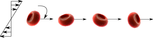
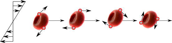
Figure 1: The two types of motion considered in modeling a RBC in a linear shear field, the solid-like, tumbling or flipping coin motion (upper panel), and the vesicular, tank-treading motion (lower panel), where two material points on the RBC membrane move at fixed body orientation.

Consequently, at rotational level, the RBC experiences two distinct components of the torque. The first one arises from the coupling between the body motion and the fluid vorticity, that we represent by the following rotational kernel

$$\boldsymbol{\tau}^{A}({\bf{\bf x}},{\bf\Gamma}_{i})=-\gamma_{R}\tilde{\delta}({\bf x}-{\bf R}_{i},{\bf Q}_{i})\left[{\bf\Omega}_{i}-{\bf\boldsymbol{\omega}}({\bf x})\right]=-\gamma_{R}\tilde{\delta}_{i}\left({\bf\Omega}_{i}-{\bf\boldsymbol{\omega}}\right)$$ (15)

where $\gamma_{R}$ is a rotational coupling coefficient and the superscript $A$ stands for antisymmetric. This term depends on the body shape and orientation via the shape function and, in a linear shear flow, generates angular motion at constant angular velocity.

The elongational component of the flow contributes to the orientational torque for bodies with ellipsoidal symmetry, being zero for spherical solutes rioual_analytical_2004. By defining the stress vector ${\bf t}^{\boldsymbol{\sigma}}=\boldsymbol{\sigma}\cdot\hat{{\bf n}}$, where $\hat{{\bf n}}$ is the outward normal to the surface of a macroscopic RBC, we replace the surface normal with the vector spanning over the entire volume of the diffused particle, $\hat{{\bf n}}=\boldsymbol{\partial}\tilde{\delta}/|\boldsymbol{\partial}\tilde{\delta}|$. The associated torque is represented in analogy with the torque acting on macroscopic bodies leal_advanced_2007, by the kernel

$$\boldsymbol{\tau}^{S}({\bf{\bf x}},{\bf\Gamma}_{i})=\alpha\tilde{\delta}_{i}{\bf t}^{\boldsymbol{\sigma}}\times({\bf x}-{\bf R}_{i})$$ (16)

where $\alpha$ is a parameter to be fixed and the superscript $S$ is mnemonic for the symmetric contribution of the flow. As shown in the following, the elongational component of the torque includes an independent contribution arising from tank treading that will allow us to tune the parameter $\alpha$ based on known data on the tumbling to tank treading transition.

The hydrodynamic force and torque acting on the RBC are obtained via integration over the globule spatial extension. Owing to the discrete nature of the mesh, the integrals are written as discrete sums,

$${\bf F}_{i} = \sum_{{\bf x}}\boldsymbol{\phi}({\bf{\bf x}},{\bf\Gamma}_{i})=-\gamma_{T}({\bf V}_{i}-\tilde{{\bf u}}_{i})$$ (17)

$${\bf T}_{i}^{A} = \sum_{{\bf x}}\boldsymbol{\tau}^{A}({\bf{\bf x}},{\bf\Gamma}_{i})=-\gamma_{R}({\bf\Omega}_{i}-\tilde{\boldsymbol{\omega}}_{i})$$ (18)

$${\bf T}_{i}^{S} = \sum_{{\bf x}}\boldsymbol{\tau}^{S}({\bf{\bf x}},{\bf\Gamma}_{i})$$ (19)

where

$$\tilde{{\bf u}}_{i} \equiv \tilde{\delta}_{i}\star{\bf u}=\sum_{{\bf x}}\tilde{\delta}_{i}{\bf u}$$ (20)

$$\tilde{\boldsymbol{\omega}}_{i} \equiv \tilde{\delta}_{i}\star\boldsymbol{\omega}=\sum_{{\bf x}}\tilde{\delta}_{i}\boldsymbol{\omega}$$ (21)

are smeared hydrodynamic fields and the symbol $\star$ denotes convolution over the mesh.

The action of the forces ${\bf F}_{i}$ and torques ${\bf T}_{i}={\bf T}_{i}^{S}+{\bf T}_{i}^{A}$ are counterbalanced by opposite reactions on the fluid side. Conservation of linear and angular momentum in the composite fluid-RBC system preserves the basic symmetries of the microdynamics and produces the consistent hydrodynamic response duenweg_lattice_2008. The action of forces and torques on the fluid populations are expressed according to the following body force

$${\bf G}=-\sum_{i}\left\{{\bf F}_{i}\tilde{\delta}_{i}+\frac{1}{2}{\bf T}_{i}\times\boldsymbol{\partial}\tilde{\delta}_{i}\right\}$$

The two exchange terms arising from the translational and rotational back-reactions produce distinct modifications of the fluid velocity and vorticity. Some algebra shows that every suspended body preserves mass and linear momentum in the composite fluid-RBC system since $\sum_{{\bf x}}\Delta{\bf u}=\sum_{{\bf x}}\sum_{p}\Delta f_{p}{\bf c}_{p}=-{\bf F}_{i}$. Similarly, every suspended body preserves the total angular momentum, since

$$\sum_{{\bf x}}\Delta\boldsymbol{\omega}=\sum_{{\bf x}}\sum_{{\bf p}}\Delta f_{p}{\bf c}_{p}\times({\bf x}-{\bf R}_{i})=\frac{1}{2}\sum_{{\bf x}}\left({\bf T}_{i}\times\boldsymbol{\partial}\tilde{\delta}_{i}\right)\times({\bf x}-{\bf R}_{i})=-{\bf T}_{i}$$ (22)

where we have used the Lagrange rule, ${\bf a}\times({\bf b}\times{\bf c})=({\bf a}\cdot{\bf c}){\bf b}-({\bf a}\cdot{\bf b}){\bf c}$ and the property of the shape function, eq. (13).

II.3 Tank Treading

Tank Treading (TT) is the motion featured by vesicles and RBC and arises from the sliding of the surrounding membrane when subjected to a shearing flow. It can be visualized by considering a material point anchored to the RBC membrane and moving in elliptical orbits while maintaining fixed the orientation of the RBC with respect to the shearing direction (see Fig. 1). The physical parameters controlling tank treading are the ratio of viscosity between plasma and the inner fluid entrained within the RBC, the shape of the RBC and the shear rate $\dot{\gamma}$ keller_motion_1982.

In modeling blood, it is essential to include TT as it acts to orient RBC with a privileged angle with respect to the flow direction. In proximity of the vessel walls, the fixed orientation induces a net lift force proportional to $\dot{\gamma}$ that pushes the globule away from the walls olla_simplified_1999. Lift forces, arising from either single-body or many-body effects, are thought to induce the Farhaeus-Lindqvist phenomenon, the drop of blood viscosity in vessels of sub-millimeter diameters, an effect with far-reaching consequences in physiology lightfoot_transport_1974.

In the general case, TT motion takes place in an apparently decoupled fashion from tumbling, as vorticity and elongational contributions have different origins. However, the motion of the rigid-body RBC is partially compensated by the movement of the surrounding membrane and thus effectively couples tumbling and TT motion via the instantaneous orientation of the globule. At small values of the viscosity ratio, orientational torques prevail over the rotational ones and pure TT motion with a fixed RBC orientation is observed. The phase diagram as a function of the viscosity ratio provides a direct view on the RBC response to shear kessler_swinging_2008.

An analytical treatment accounting for tank treading is due to Skalak and Keller (SK) keller_motion_1982 a model that has enjoyed a large popularity in determining the single-body forces and torques acting on RBCs messlinger_dynamical_2009 . Recently the SK model has been re-derived by Rioual et al. rioual_analytical_2004 via a heuristic argument that we recall here. In 2D, when the RBC is subjected to a velocity field ${\bf u}=(0,\dot{\gamma}y)$, the elongational component tends to align the RBC along the shearing principal eigenvector. For an elliptical body, the alignment has an angle $\psi=\frac{\pi}{4}$, where $\psi$ is the angle formed by the RBC largest principal axis with respect to the flow direction.

In general, the torque acting on a RBC can be decomposed into three separate components. The first component is due to the angular motion of RBC in a quiescent fluid and produces a frictional torque given by $-\gamma_{R}\boldsymbol{\Omega}$, where $\gamma_{R}$ is a phenomenological coefficient that can be identified with the one introduced in eq.(15). The second component is due to the torque from the shearing fluid on the quiescent RBC and for a quiescent membrane, being related to the vorticity component of the flow. The analytical solution for the 2D elliptical RBC without TT motion provides a total torque proportional to $\dot{\gamma}\left(\frac{L_{1}^{2}+L_{2}^{2}}{2}+\frac{L_{1}^{2}-L_{2}^{2}}{2}\cos 2\psi\right)$, where $L_{1,2}$ are two shape-dependent coefficients and where the first term of the expression is associated to vorticity while the second term to the elongational component of the flow. The latter provides two equilibrium positions for $\psi=\pm\frac{\pi}{4}$ and maximal torque for $\psi=0,\frac{\pi}{2}$.

Finally, the effect of tank treading is determined by considering the local frame moving together with the material point at velocity ${\bf V}_{TT}$ and with the infinitesimal membrane element experiencing a force $d{\bf F}_{TT}\propto{\bf V}_{TT}$ and torque $\boldsymbol{\tau}_{TT}=\oint d{\bf F}_{TT}\times({\bf x}-{\bf R})$. Consequently, TT couples to both the rotational and elongational flow components and results in a net torque $\boldsymbol{\tau}_{TT}\propto\cos(2\psi)$, that is, a torque enjoying the same angular symmetry of the mechanism associated to the rigid body response. Given the three-dimensional, diffused nature of the numerical model, the actual presence of the cellular membrane is not explicitly considered. Instead, the effect of TT is controlled by tuning the intensity of the elongational torque via the adimensional factor $\alpha$ of eq. (16).

II.4 Viscosity contrast

RBC are carriers of an internal fluid composed of several hundred millions of hemoglobin proteins and being much more viscous than plasma. The inner fluid contributes significantly to the dissipation of energy as mediated by the shearing modes activated by the RBC membrane. The consequence is the steep raise in the apparent viscosity with the hematocrit level. We incorporate the effect of the viscosity contrast by considering a local enhancement of the LB fluid viscosity within the RBC shape according to the following BGK relaxation time

$${\cal T}(x)={\cal T}_{0}+\Delta h\sum_{i}\tilde{\theta}_{i}$$ (23)

where ${\cal T}_{0}$ corresponds to the viscosity of pure plasma, $\Delta$ is viscosity enhancement factor, and $\tilde{\theta}_{i}$ is a smooth version of the ellipsoidal characteristic function. The latter is represented as $\tilde{\theta}_{i}=1-(1-\tilde{\delta_{i}})^{\kappa}$ where the parameter $\kappa$ governs the smooth transition between the inner and outer fluids, chosen as $\kappa=20$. By choosing $\nu_{0}=1/6$ and $\Delta=2$, the ratio between inner ($\tilde{\theta}_{i}\sim 1$) and outer ($\tilde{\theta}_{i}\sim 0$) viscosities is equal to $5$.

II.5 Excluded Volume Interactions

In order to account for the RBC-RBC repulsive forces, soft-core mechanical forces and torques are given by the Gay-Berne (GB) potential gay_modification_1981, as widely used in the liquid crystals community. The GB potential inhibits interpenetration of pairs of RBCs by introducing an orientation-dependent repulsive interaction derived from the Lennard-Jones potential ($\phi_{LJ}(R_{ij})=\epsilon[(\sigma/R_{ij})^{12}-(\sigma/R_{ij})^{6}]$, where $\epsilon$ is the energy scale and $\sigma$ the “contact” length scale). The GB potential extends the spherically symmetric Lennard-Jones potential to ellipsoidal symmetry, where the potential depends if two RBCs have mutual orientation as face-to-face (maximal repulsion), side-to-side (minimal repulsion) or an arbitrary orientation between the two bodies (intermediate case).

In the following, we shall employ the form of the GB potential that handles the interaction between particles of different eccentricity, such as a mixture of ellipsoidal and spherical particles. This flexibility allows to handle biofluids composed of particles with different shapes by employing the same analytical form of the potential.

Given the principal axes $(a_{i,1},a_{i,2},a_{i,3})$ of the $i$-th globule, the ellipsoidal shape associated to the excluded volume interactions is constructed according to the shape matrix $S_{i}=\mbox{{diag}}(a_{i,1},a_{i,2},a_{i,3})$ and the transformed matrix ${\bf A}_{i}={\bf Q}_{i}{\bf S}_{i}^{2}{\bf Q}_{i}^{T}$ in the laboratory frame. The pair of particles $i,j$ at distance ${\bf R}_{ij}$ experiences a characteristic exclusion distance $\sigma_{ij}$ that depends on the globule-globule distance, shape and mutual orientation, written as

$$\sigma_{ij} = \frac{1}{\sqrt{\phi_{ij}}}$$ (24)

$$\phi_{ij} = \frac{1}{2}\hat{{\bf R}}_{ij}\cdot{\bf H}_{ij}^{-1}\cdot\hat{{\bf R}}_{ij}$$ (25)

where the matrix ${\bf H}_{ij}={\bf A}_{i}+{\bf A}_{j}$ has been introduced.

A purely repulsive exclusion potential is given by the pairwise form gay_modification_1981; allen_expressions_2006

$$u_{ij}=\left\{\begin{array}[]{lc}4\epsilon_{0}(\rho_{ij}^{-12}-\rho_{ij}^{-6})+\epsilon_{0}&\qquad\rho_{ij}^{6}\leq 2\\ 0&\qquad\rho_{ij}^{6}>2\end{array}\right.$$ (26)

with

$$\rho_{ij}=\frac{R_{ij}-\sigma_{ij}+\sigma_{ij}^{min}}{\sigma_{ij}^{min}}$$ (27)

where $\epsilon_{0}$ is the energy scale and $\sigma_{ij}^{min}$ is a constant, both parameters being independent on the ellipsoidal mutual orientation and distance. For two identical oblate ellipsoids, $\sigma_{ij}^{min}$ corresponds to a contact distance of the two particles having face-to-face orientation. In general, by considering the minimum particle dimension $a_{i}^{min}=\min(a_{i,1},a_{i,2},a_{i,3})$ then

$$\sigma_{ij}^{min}=\sqrt{2\left[\left(a_{i}^{min}\right)^{2}+\left(a_{j}^{min}\right)^{2}\right]}$$ (28)

The mutual forces and torques exerted between the $i,j$ pair are computed accordingly, as described in the appendix for the sake of completeness.

We note here two aspects. First, the softness of the RBC can be improved by taking small values for the energy scale $\epsilon_{0}$. Clearly, this type of softness does not arise from hydrodynamic forces but from RBC-RBC mechanical forces, and emulates the good packing attitude of RBCs at high hematocrit levels. Secondly, the ellipsoidal exclusion shape can be modified to reproduce more closely the biconcave discoid via the Bates-Lockhurst version of the GB potential care_computer_2005. At present, we take the ellipsoidal shape to be representative of RBC, while further refinements can be trivially included.

When simulating blood flows in a confining environment, we associate to each wall mesh point a spherical particle that acts as a repulsive center for the ellipsoidal RBC and prevents the globule from leaking out of the confining vessel, under the action of the same GB potential. The wall-RBC characteristic distance $\sigma_{w,RBC}^{min}$ is chosen to be half the mesh spacing $\frac{\Delta x}{2}$.

II.6 Summary of the computational model

To recap, the basic assumption of the model is to handle a suspension made of plasma and RBC. The former is a Newtonian fluid that reproduces Navier-Stokes dynamics at virtually arbitrary Reynolds numbers and in arbitrary geometries. The physiological conditions of Reynolds $\lesssim 2000$ and shear rates $\lesssim 500\,s^{-1}$ can be accessed in simulation without posing limitations in terms of numerical robustness and feasibility. The model for RBCs has the following characteristics:

• it is based on the body forces and torques acting on the RBC rather than on surface forces by a proper decomposition of the translational, tumbling and orientational components of the flow. A similar scenario is found in Faxen’s law for zero-Reynolds flows leal_advanced_2007. Our strategy does not track explicitly the RBC membrane or handle in anyway the internal cytoskeleton;

• RBCs are active scalars with hydrodynamic shape that is fixed and ellipsoidal. The eccentricity of the RBC can be tuned, however in the following we choose to work with $\xi_{x}=1$ and $\xi_{y}=\xi_{z}=2$, corresponding to volume $V\simeq 134$, surface $S\simeq 139$ and reduced volume $v\equiv\frac{3V}{4\pi(S/4\pi)^{3/2}}\simeq 0.87$, that should be compared with $v=0.65$ for human RBCs;

• The near-field hydrodynamic interactions are well captured by the model, in particular as regarding to translational and orientational mobilities and long-time tails arising from hydrodynamic interactions. Shape fluctuations can be easily introduced, e.g. by means of the Maffettone-Minale extension maffettone_equation_1998, by allowing volume-preserving deformations while still maintaining the ellipsoidal symmetry;

• the viscosity contrast is introduced by allowing for a modification of the relaxation time within the RBC region. In practice, this means solving the same LB algorithm throughout the system, but with a local relaxation time and thus, higher dissipation within the RBC region. In terms of computational feasibility, a wide range of viscosity contrast can be explored, but in the following we will focus on a given viscosity contrast as pertaining to RBCs;

• interpenetration between RBCs is avoided by Gay-Berne forces and torques. The degree of softness of particles can be tuned, as much as some attracting component of the interaction due to adhesive forces or the presence of fibrinogen, can be easily accommodated within the model.

In summary, the main assumption of the model, the neglect of shape fluctuations, is largely compensated by its main strength, the possibility to handle large-scale systems of physiological relevance with state-of-the-art computer hardware. This is a major point of the model that will not be addressed in detail here, but has been discussed in refs.bernaschi_muphy:_2009; bernaschi_flexible_2010; peters_multiscale_2010.

III Numerical Results

The frictional response of a single RBC in plasma is first analyzed by computing the Stokes response of an oblate ellipsoidal particle having two possible orientations with respect to the motion direction. For translational displacement, these are the frontal and side-wise motions. For the rotational motion, these correspond to spinning around two principal directions corresponding to the smallest and largest radii. For this preliminary test, we deactivate the modulation of viscosity by the presence of the RBC, that is, we take the same viscosity for plasma and the entrained fluid without distinction and throughout the simulation domain.

As shown in ref. ahlrichs_simulation_1999 for a model of suspended point-like particles, the effective mobility is given by the sum of two components, the mobility associated to the bare frictional parameters, $\gamma_{T}$ and $\gamma_{R}$, and the effect of the hydrodynamic field induced on the surrounding solvent that sustains the motion by increasing the particle roto-translational mobilities. In addition, the hydrodynamic components to mobility contains a Stokes-like component that is renormalized by the presence of the numerical finite-spacing mesh. We expect to recover the same qualitative behavior for the diffused ellipsoidal particles.

Fig.2 shows the computed particle mobilities as a function of the frictional parameters $\gamma_{R}$ and $\gamma_{T}$ for a RBC of mass $M=10$ and inertia $I_{x,y,z}=1000$ (all data are expressed in lattice units unless otherwise stated). The particle is embedded in a simulation box of size $60\times 60\times 60$ containing a quiescent fluid. At infinite friction, the intercepts correspond to the mesh-induced spurious frictional forces. For translational motion, the intercepts correspond to two mobilities, $\mu\equiv\frac{1}{M\gamma_{T}^{mesh}}=6.6$ and $10.3$, for frontal and side-wise translation motion, respectively. By associating a residual hydrodynamic radius $a_{T}^{mesh}=\frac{M\gamma_{T}^{mesh}}{6\pi\nu\rho}=0.06$ and $0.03$ to frontal and side-wise motion, respectively, it is apparent that the residual radius is directly proportional to the size factor $\xi_{\alpha}$ governing the shape function. From these data it is clear that the residual Stokes radii are much smaller than the mesh spacing (being $\Delta x=1$ in lattice units) and modulating the hydrodynamic response to achieve a bulkier suspended body requires increasing the coupling parameter to $\gamma_{T}>10$. High values of $\gamma_{T}$ spoil the numerical robustness of the method. In fact, a simple estimate shows that numerical stability of the LB method is for body forces $|F|\lesssim 0.1$, that is $\gamma_{T}\lesssim 0.1$. The translational data show that the coupling method alone reproduces the far-field Stokes response but is unable to modulate the viscosity to significant values with the hematocrit level, unless a different mechanism is introduced to improve the internal dissipation, such as the one encoded by eq. (23).

For angular motion, the situation is slightly different since we find the intercepts $\gamma_{R}^{mesh}=\frac{1}{44}\,\Delta t^{-1}$ and $\frac{1}{38}\,\Delta t^{-1}$ for rotations around the smallest and largest principal radii, respectively. The intercepts correspond to the residual rotational radii $a_{R}^{mesh}=\left(\frac{I\gamma_{R}^{mesh}}{8\pi\nu\rho}\right)^{1/3}=1.84\,\Delta x$ and $1.75\,\Delta x$, respectively. In the angular motion, the mesh-induced friction is larger than the translational counterpart (in fact, comparable to the mesh spacing) and exhibits a weak dependence on the direction of spinning direction, so that it can be considered independent on the latter.

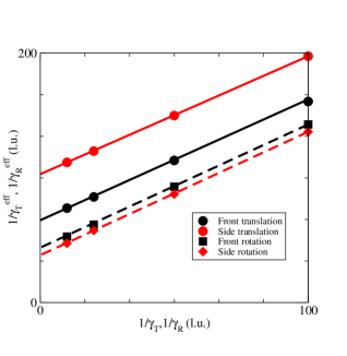
Figure 2: Translational and rotational mobilities as a function of the coupling parameters $\gamma_{T}$ and $\gamma_{R}$. Circles correspond to frontal (filled symbols) and lateral translation (open symbols). Squares are for rotations around the smallest principal radius (filled symbols) and around the largest principal radius (open symbols). The lines are guides for the eye.

The effect of tank treading is analyzed by placing a RBC in a shear field generated according to the method of ref. wagner_lees-edwards_2002. Fig. 3 shows the time dependence of the elongational component of the torque for a single RBC in a shear flow. Different values of the enhancement factor $\alpha$ are reported having chosen $\gamma_{T}=\gamma_{R}=10^{-1}$. It is found that the value $\alpha=0.063$ corresponds to the transition to pure TT motion, where the elongational and vorticity-related torques exactly compensate, generating a constant orientation with angle $\simeq 40^{o}$ as a fixed point of the dynamics. For a bounded fluid in a two-dimensional slab the fixed angle is found to be in the range $20^{o}-35^{o}$, depending on the viscosity contrast and flow curvature, with a lift force being linearly proportional to the local shear rate and to $y^{-2}$, where $y$ is the distance of the RBC from the wall, in agreement with experimental and theoretical results cantat_lift_1999; coupier_noninertial_2008.

Overall, the torques generate a well-behaved rotational motion and in line with the expected trend. In the following we arbitrarily set the tunable parameter $\alpha=0.04$, that is, slightly below the transition to tank treading, and proceed further with tests regarding the rheological response of a dense suspension. The tests in the bounded fluid confirm the tumbling regime for the chosen RBC shape and viscosity ratio. It should be borne in mind that the balance between tumbling and tank treading in a dilute suspension critically affects the lift forces and thus the viscosity of the suspension danker_rheology_2007. In this respect, the fixed-shape approximation of the present model produces hydrodynamic forces that are qualitatively correct. In the future, the model can be tuned more finely by optimizing the shape and viscosity contrast.

Figure 3: Symmetric component of the torque of a single RBC in a shear field and for different values of the tank treading parameter $\alpha$.

The viscosity of the suspension is computed by using a cylindrical channel of radius $50\,\mu m$ and for different hematocrit levels. In Fig. 4 we report the relative viscosity ($\eta_{rel}=\eta_{app}/\eta_{0})$ where $\eta_{app}$ is the apparent viscosity measured in the channel at finite hematocrit and $\eta_{0}$ the viscosity in the same channel at zero hematocrit. Since $\eta\propto Q$, where $Q$ is the volumetric flow rate, $\eta_{rel}$ is computed as the ratio of flow rates at finite and zero hematocrit. Fig. 4 also reports the data on viscosity by setting the enhancement factor of eq. (23) to $\Delta=0$. The latter produce a weak modulation of viscosity with hematocrit, while the data with $\Delta=2$ exhibit an excellent agreement with the experimental results of ref. pries_blood_1992.

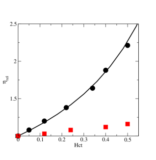
Figure 4: Relative viscosity in a channel of radius $50\,\mu m$ for different hematocrit levels as compared to the experimental data of Pries et al. pries_blood_1992(solid curve). Data are for the enhanced dissipation mechanism of eq. (23) with $\Delta=2$ (circles) and without enhancement ($\Delta=0$) (squares).

A crucial phenomenology of blood circulation is the decrease of viscosity as the vessel radius falls below $100\,\mu m$, namely, the Farhaeus-Lindqvist effect lightfoot_transport_1974. This effect is usually ascribed to the formation of a cell-free layer in proximity of the vessel walls. The origin of such depletion is still uncertain but the lateral forces that push the RBCs away from the vessel walls are retained to have different causes, such as tank treading and cell deformation olla_simplified_1999, adhesive properties of RBC or shear-induced migration. In the current version of our model, we do not probe the effects of cell deformation. However, the simulation reveals a distinct RBC depletion in proximity of the walls, as shown in Fig. 5. We report the variation of the cell-free layer with the hematocrit and vessel diameter as compared to the experimental data of Bugliarello and Sevilla bugliarello_velocity_1970. The numerical results reproduce the experimental data quite well, lending good confidence in the numerical model at vessel diameters below the $100\,\mu m$ radius. The typical cell-free layer observed in simulation for two channels of different radii is illustrated in Fig. 5, inset. The progressive depletion of RBC as compared to the plasma content is the leading cause of fluidization of the suspension at small channel radius.

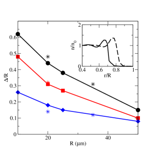
Figure 5: Size dependence of the cell-free layer with the vessel diameter and hematocrit level of $10\,\%$ (diamonds), $20\,\%$ (squares) and $50\,\%$ (circles), as compared to the experimental data of Bugliarello and Sevilla bugliarello_velocity_1970 (star symbols). The lines are guides for the eye. Inset: Radial density profiles of RBC, for $R=10\,\mu m$ (solid line) and $R=20\,\mu m$ (dashed line), illustrating the cell-free layers in proximity of the vessel wall.

The non-Newtonian behavior of the suspension is further exhibited by the velocity profiles of RBC for different hematocrit levels and vessel diameters, as shown in Fig. 6. As the hematocrit level increases, the Poiseuille-like parabola modifies into flatter profiles next to the vessel centerline and in a large extension of the channel, whereas in proximity of the walls, the profiles have large slopes and strong dissipation, in particular for the narrower vessels. We further notice a good match of the plasma and RBC velocities for all vessel radii, a matching that is typically lost as the vessel radius becomes comparable to the RBC size (data not shown).

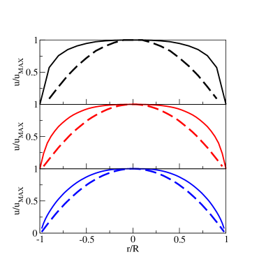
Figure 6: Velocity profiles for vessel radius of $10$ (upper panel), $25$ (mid panel) and $50\,\mu m$ (lower panel). Data correspond to hematocrit levels of $35\%$ (solid lines) and $0\%$ (dashed lines).

In applying the model to physiological conditions, we consider a realistic bifurcating vessel at $50\%$ hematocrit level, as depicted in Fig. 7. The bifurcation is extracted as part of a coronary arterial system melchionna_hydrokinetic_2010, and is made of a parent vessel of radius $\sim 100\,\mu m$ and one daughter branch having approximately the same size of the parent vessel, and a second daughter branch of radius $\sim 80\,\mu m$.

The flow is induced by imposing parabolic flow conditions at the inlet and constant pressure at the outlets, with the method described in peters_multiscale_2010, producing a shear rate of $80\,s^{-1}$ averaged over the entire bifurcation at steady state, and reaching as high as $150\,s^{-1}$ in proximity of the arterial wall, values in line with the typical shear rates observed in human coronary arteries, typically in the $30-450\,s^{-1}$ range ethier_introductory_2007. As the snapshot reveals, RBCs organize in several different ways throughout the bifurcation and also depending on the value of the shear rate (data not shown). The local organization of RBCs in rouleaux is clearly visible, the typical stack often observed in static or flow conditions, and mostly destroyed as the shear rate increases.

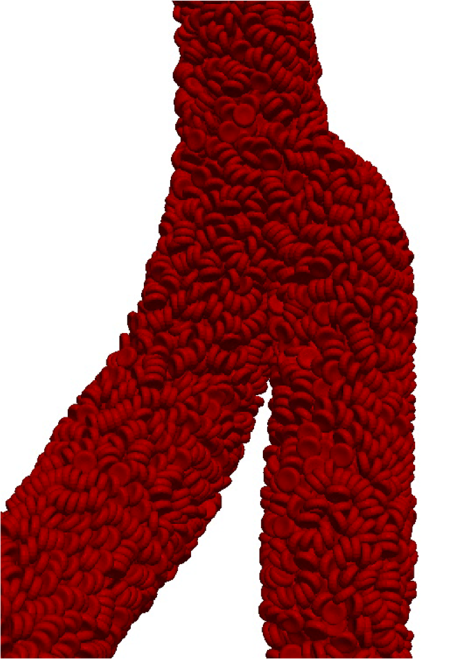
Figure 7: Snapshot of the bifurcating vessel showing the organization of RBCs at hematocrit of $50\,\%$ and average shear rate of $80\,s^{-1}$.

The flow in the bifurcating channel for different values of the shear rate is analyzed and the shear thinning behavior is illustrated in Fig. 8, where viscosity decreases with the shear rate until the Newtonian plateau is reached.

As expected, shear thinning correlates with the formation of rouleaux, as seen by inspecting the statistical distribution of cluster size. The histogram of the rouleaux size is reported in Fig. 8, inset. As shear rate increases, fewer and smaller structures are detected. However, a central observation is that the local structuring of RBCs strongly depends on the morphological details of the vessel. In fact, we notice that in proximity of the bifurcation a shoulder in a daughter vessel creates smaller flow velocity and some stagnation of RBCs. In correspondence of this region, rouleaux show resilient character even for shear rates above $50\,s^{-1}$.

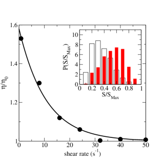
Figure 8: Shear thinning of the suspension in the bifurcating channel for different values of the shear rate. Inset: Distribution of rouleaux as a function the cluster size $S$, for shear rate of $8\,s^{-1}$ (solid bars) and $16\,s^{-1}$ (open bars).

The uneven distribution of RBCs, with the attendant stagnation and persistence of rouleaux in specific regions, can have significant impact on the distribution of shear stress. The latter quantity strongly correlates with the formation of plaques in the endothelium (atherogenesis) and the subsequent development of atherosclerosis rybicki_prediction_2009. In particular, low levels of shear stress, as due to disturbed flow patterns and stagnation regions, trigger the growth of plaques. It is therefore of great relevance to inspect the role of RBCs in modulating the shear stress distribution on the wall of the vessel under study.

For this analysis, we employ the method described in ref. melchionna_hydrokinetic_2010 and compute the endothelial shear stress as time averages over the evolution of the plasma-RBC composite system. Fig. 9 illustrates the distribution of shear stress for different hematocrit levels. The plot reveals the strong effect of the RBCs throughout the system and in particular the great fluctuations in one daughter vessel. While the overall shear stress distribution is somehow preserved at different hematocrit levels, important local modifications are induced by RBCs. In particular, in proximity of the vessel shoulder, the RBC structuring induces smaller values of the shear stress, followed by larger values next to the inner side of the bifurcation. Given these observations, it is expected that the particulate nature of blood has significant effects in the identification and prediction of vulnerable regions of the large-size vascular system by computational methods.

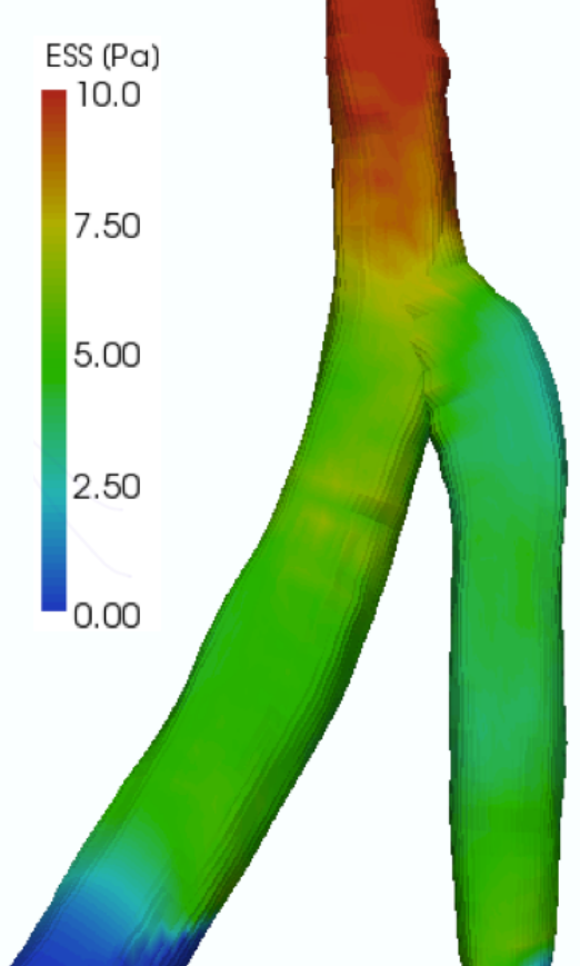
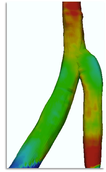
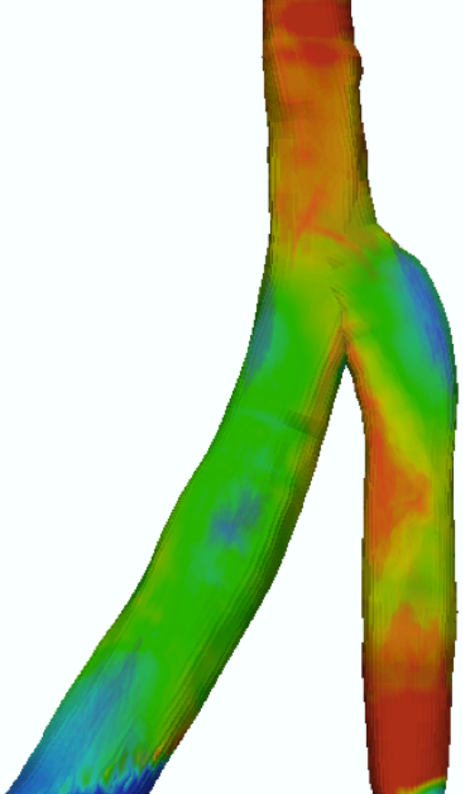
Figure 9: Time-averages of shear stress in the bifurcating channel for pure plasma (left panel), hematocrit level of $35\,\%$ (mid panel) and $50\,\%$ (right panel). The flow corresponds to an average shear rate of $80\,s^{-1}$.

IV Conclusions

In this paper, a new model for suspended red blood cells has been introduced with the goal of studying large-scale hemodynamics in cardiovascular systems. The underlying idea is to represent the different responses of the suspended bodies, emerging from the rigid-body as much as the vesicular nature of the globule, by distinct coupling mechanisms. These mechanisms are entirely handled at kinetic level, that is, the dynamics of plasma and red blood cells is governed by appropriate collisional terms that avoid to compute hydrodynamic forces and torques via the Green’s function method, as employed in Stokesian dynamics brady_stokesian_1988. The fundamental advantage of hydrokinetic modeling is to avoid such expensive route and, at the same, enabling to handle finite Reynolds conditions and complex boundaries or irregular vessels within the simple collisional approach. At macroscopic scale, the non-trivial rheological response emerges spontaneously as a result of the underlying microdynamics.

The second, crucial advantage of the proposed method is to enable the investigation of systems of physiological relevance whose phenomenology typically spans several decades in time and space. To this purpose, massive parallel computers must be deployed by exploiting a numerical method that scales over thousands of processors and above. To a large extent, both the Lattice Boltzmann method and the red blood cell dynamics have been proved to scale over traditional CPU-based computers such as on Blue Gene architectures, as much as over massive assemblies of Graphic Processing Units (see ref. peters_multiscale_2010 and references therein).

The numerical results presented in this paper have shown that the particulate nature of blood cannot be omitted when studying the non-trivial rheology of the biofluid and the shear stress distribution in complex geometries. Regions of low shear stress can appear as the hematocrit reaches physiological levels as a result of the non-trivial organization of red blood cells and the irregular morphology of vessels. These results cannot can have far reaching consequences in real-life cardiovascular applications, where the organization of red blood cells impacts both the local flow patterns and the large-scale flow distribution in complex vascular networks.

Appendix A Rigid Body Dynamics

We report here the numerical solution of the roto-translational dynamics for RBCs. The rotational dynamics is customarily solved in the body frame where the equation relating angular momentum $\boldsymbol{\pi}$ and angular velocity ${\bf\Omega}$ is

$$\boldsymbol{\pi}={\bf I}\boldsymbol{\Omega}$$ (29)

where, for ease of notation, we have omitted the RBC index. The rigid-body dynamics is given by

$$\dot{\boldsymbol{\Omega}}={\bf I}^{-1}\left[({\bf I}\boldsymbol{\Omega})\times\boldsymbol{\Omega}\right]+{\bf I}^{-1}\boldsymbol{\tau}$$ (30)

and the rotational matrix obeys the equation

$$\dot{{\bf Q}}={\bf Q}\,skew(\boldsymbol{\Omega})$$ (31)

where, for a vector with components ${\bf v}=(v_{n},v_{t},v_{g})$, $skew({\bf v})$ denotes

$$skew({\bf v})=\left(\begin{array}[]{ccc}0&v_{g}&-v_{t}\\ -v_{g}&0&v_{n}\\ v_{t}&-v_{n}&0\end{array}\right)$$ (32)

In absence of hydrodynamic forces and torques, the dynamics is Hamiltonian and the updating algorithm is given by the scheme described in ref. [dullweber_symplectic_1997]. For $\gamma_{T}=\gamma_{R}=0$ the algorithm is symplectic and provides excellent conservation of energy. In presence of hydrodynamic forces and torques, the algorithm is generalized as in the following steps:

1. Propagate linear and angular momenta for half-step according to the combination of mechanical and hydrodynamic forces ${\bf F}^{comb}$ and torques $\boldsymbol{\tau}^{comb}$ ,

   $${\bf\Omega}_{h/2} = {\bf\Omega}_{0}+\frac{h}{2}{\bf I}^{-1}\boldsymbol{\tau}_{0}^{comb}$$ (33)

   $${\bf V}_{h/2} = {\bf V}_{0}+\frac{h}{2M}{\bf F}_{0}^{comb}$$ (34)

   where

   $${\bf F}_{0}^{comb} = {\bf F}_{0}^{mech}+\gamma_{T}M\tilde{{\bf u}}_{0}$$ (35)

   $$\boldsymbol{\tau}_{0}^{comb} = \boldsymbol{\tau}_{0}^{mech}+\gamma_{R}{\bf I}\tilde{\boldsymbol{\omega}}_{0}$$ (36)

2. Update linear and angular momenta for half-step according to the frictional forces

   $${\bf\Omega}_{h/2} = e^{-\gamma_{R}h/2}{\bf{\bf\Omega}}_{0}$$ (37)

   $${\bf V}_{h/2} = e^{-\gamma_{T}h/2}{\bf V}_{0}$$ (38)

3. Propagate positions as

   $${\bf R_{h}}={\bf R}_{0}+h{\bf V}_{h/2}$$ (39)

4. Update the angular state by taking the rotation matrix ${\bf{\cal R}}(\alpha,\beta,\gamma)$, associated to rotation around the axes $\hat{{\bf n}}$, $\hat{{\bf t}}$ and ${\bf\hat{g}}$ with angles $\alpha$, $\beta$ and $\gamma$, respectively. Propagate the rotational state according to the sequence of five sub-rotations

   1. ${\bf{\cal R}}\equiv{\cal R}(\frac{h\alpha}{2},0,0)\longrightarrow\begin{cases}\begin{array}[]{c}{\bf\Omega}={\bf I}^{-1}{\bf{\cal R}}{\bf I}{\bf\Omega}\\ {\bf Q}={\bf Q}{\bf{\cal R}}^{\dagger}\end{array}\end{cases}$

   2. ${\bf{\cal R}}\equiv{\cal R}(0,\frac{h\beta}{2},0)\longrightarrow\begin{cases}\begin{array}[]{c}{\bf\Omega}={\bf I}^{-1}{\bf{\cal R}}{\bf I}{\bf\Omega}\\ {\bf Q}={\bf Q}{\bf{\cal R}}^{\dagger}\end{array}\end{cases}$

   3. ${\bf{\cal R}}\equiv{\cal R}(0,0,h\gamma)\longrightarrow\begin{cases}\begin{array}[]{c}{\bf\Omega}={\bf I}^{-1}{\bf{\cal R}}{\bf I}{\bf\Omega}\\ {\bf Q}={\bf Q}{\bf{\cal R}}^{\dagger}\end{array}\end{cases}$

   4. ${\bf{\cal R}}\equiv{\cal R}(0,\frac{h\beta}{2},0)\longrightarrow\begin{cases}\begin{array}[]{c}{\bf\Omega}={\bf I}^{-1}{\bf{\cal R}}{\bf I}{\bf\Omega}\\ {\bf Q}={\bf Q}{\bf{\cal R}}^{\dagger}\end{array}\end{cases}$

   5. ${\bf{\cal R}}\equiv{\cal R}(\frac{h\alpha}{2},0,0)\longrightarrow\begin{cases}\begin{array}[]{c}{\bf\Omega}={\bf I}^{-1}{\bf{\cal R}}{\bf I}{\bf\Omega}\\ {\bf Q}={\bf Q}{\bf{\cal R}}^{\dagger}\end{array}\end{cases}$

5. Compute the mechanical forces and torques from the excluded volume interactions, ${\bf F}_{h}^{mech}$ and $\boldsymbol{\tau}_{h}^{mech}$ and the fluid velocity and vorticity via Eqs.(20-21), and construct the combinations

   $${\bf F}_{h}^{comb} = {\bf F}_{h}^{mech}+\gamma_{T}M\tilde{{\bf u}}_{h}$$ (40)

   $$\boldsymbol{\tau}_{h}^{comb} = \boldsymbol{\tau}_{h}^{mech}+\gamma_{R}{\bf I}\tilde{\boldsymbol{\omega}}_{h}$$ (41)

6. Update linear and angular momenta for half-step according to the frictional forces

   $${\bf\Omega}_{h} = e^{-\gamma_{R}h/2}{\bf{\bf\Omega}}_{h/2}$$ (42)

   $${\bf V}_{h} = e^{-\gamma_{T}h/2}{\bf V}_{h/2}$$ (43)

7. Finalize the linear and angular momenta for half-step according to combined forces and torques

   $${\bf V}_{h} = {\bf V}_{h/2}+\frac{h}{2M}{\bf F}_{h}^{comb}$$ (44)

   $${\bf\Omega}_{h} = {\bf\Omega}_{h/2}+\frac{h}{2}{\bf I}^{-1}\boldsymbol{\tau}_{h}^{comb}$$ (45)

Appendix B Gay-Berne forces and torques

The calculation of mechanical forces and torques according to the Gay-Berne potential, eq. (26), is reported here. For the interacting pair $i,j$ , the pairwise mechanical force is given by

$${\bf{\bf F}}_{ij}^{GB}=-\frac{\partial u_{ij}}{\partial R_{ij}}\hat{{\bf R}}_{ij}-\frac{1}{R_{ij}}\frac{\partial u_{ij}}{\partial\phi_{ij}}\frac{\partial\phi_{ij}}{\partial\hat{{\bf R}}_{ij}}\cdot\left({\bf 1}-\hat{{\bf R}}_{ij}\hat{{\bf R}}_{ij}\right)=-\frac{\partial u_{ij}}{\partial R_{ij}}\hat{{\bf R}}_{ij}-\frac{1}{R_{ij}^{2}}\frac{\partial u_{ij}}{\partial\phi_{ij}}\left[\boldsymbol{\kappa}_{ij}-(\boldsymbol{\kappa}_{ij}\cdot\hat{{\bf R}}_{ij})\hat{{\bf R}}_{ij}\right]$$ (46)

where the following vector has been defined

$$\boldsymbol{\kappa}_{ij}={\bf H}_{ij}^{-1}\cdot{\bf R}_{ij}$$ (47)

The terms appearing in eq. (46) are computed as

$$\frac{\partial u_{ij}}{\partial R_{ij}}=-24\epsilon_{0}\left[\frac{\left(2\rho_{ij}^{-13}-\rho_{ij}^{-7}\right)}{\sigma_{ij}^{min}}\right]$$ (48)

and

$$\frac{\partial u_{ij}}{\partial\phi_{ij}}=-24\epsilon_{0}\left[\frac{\left(2\rho_{ij}^{-13}-\rho_{ij}^{-7}\right)\sigma_{ij}^{3}}{2\sigma_{ij}^{min}}\right]$$ (49)

The torques are calculated according to the prescription in ref. [allen_expressions_2006] and transformed back to the body frame

$$\boldsymbol{\tau}_{i}^{GB}={\bf Q}_{i}^{T}({\bf R}_{ci}\times{\bf f}_{\kappa_{ij}})$$ (50)

and

$$\boldsymbol{\tau}_{j}^{GB}={\bf Q}_{j}^{T}({\bf R}_{cj}\times{\bf f}_{\kappa_{ij}})$$ (51)

where

$${\bf f}_{\kappa_{ij}}=-\frac{1}{R_{ij}}\frac{\partial u_{ij}}{\partial\phi_{ij}}\boldsymbol{\kappa}_{ij}$$ (52)

and

$${\bf R}_{ci} = {\bf R}_{c}-{\bf R}_{i}$$

$${\bf R}_{cj} = {\bf R}_{c}-{\bf R}_{j}$$

$${\bf R}_{c} = {\bf R}_{i}-{\bf A}_{i}\boldsymbol{\kappa}_{ij}$$

It is easy to show that torques obey conservation of angular momentum since $\boldsymbol{\tau}_{i}^{GB}+\boldsymbol{\tau}_{j}^{GB}=-{\bf R}_{ij}\times{\bf F}_{ij}^{GB}$.