Padé–type rational and barycentric interpolation

Abstract

In this paper, we consider the particular case of the general rational Hermite interpolation problem where only the value of the function is interpolated at some points, and where the function and its first derivatives agree at the origin. Thus, the interpolants constructed in this way possess a Padé–type property at 0. Numerical examples show the interest of the procedure. The interpolation procedure can be easily modified to introduce a partial knowledge on the poles and the zeros of the function to approximated. A strategy for removing the spurious poles is explained. A formula for the error is proved in the real case. Applications are given.

Keywords:Rational interpolation Padé–type approximation barycentric formula piecewise rational interpolation.

Mathematics Subject Classification: 65D05, 65D15, 41A20, 41A21.

1 Padé–type approximation and rational interpolation

For representing a function $f$, rational functions are usually more powerful than polynomials. The information on the function $f$ can consist either in the first coefficients of its Taylor series expansion around zero, or in its values at some points of the complex plane.

In the first case, Padé–type, Padé, or partial Padé approximants can be used. They are rational functions whose series expansion around zero (obtained by Euclidean division in ascending powers of the numerator by the denominator) coincides with the series $f$ as far as possible. In Padé–type approximation, the denominator can be arbitrarily chosen and, then, the coefficients of the numerator are obtained by imposing the preceding approximation–through–order conditions. In Padé approximation, both the denominator and the numerator are fully determined by these conditions. For partial Padé approximants, a part of the denominator and/or a part of the numerator can be arbitrarily chosen, and their remaining parts are given by the approximation–through–order conditions. On these topics, see [7, 13, 14, 1].

In the second case, an interpolating rational function can be built using Thiele’s formula, which comes out from continued fractions (see, for example, [12, pp. 102ff.] or [15, Sec. III.3–4]). It achieves the maximum number of interpolation conditions, and, so, no choice is left for its construction [12]. The same is true for Hermite rational interpolants, a subject treated in many publications (see, for example, [26]) which is related to Newton–Padé approximants [15, p. 157]. On the other hand, when the degrees of the denominator and of the numerator are the same, writing the rational interpolant in a barycentric form allows to freely choose the weights appearing in this formula. These weights can be chosen by imposing various additional conditions such as monotonicity or the absence of poles [3, 2, 17, 4].

For an interesting discussion between the coefficients of the interpolating rational function and the weights of its barycentric representation, see [5]. For the important problems of the ill–conditioning of rational interpolation, and of the numerical stability of the algorithms for its solution, consult [5, 18].

In this paper, we will construct for the first time rational functions possessing both properties, that is interpolating $f$ at some points of the complex plane, and whose series expansion around zero coincides with the Taylor series $f$ as far as possible. Of course, this case is a particular instance of the general rational Hermite interpolation problem treated in its full generality in [26], for example. Then, using a different number of conditions than required, we are able to construct rational interpolants in the least squares sense. We will also show how information on the poles and the zeros of $f$ could be included into these interpolants in a style similar to the definition of the partial Padé approximants [8].

2 Problem statement

We consider two different arguments.

• Let $f$ be a function whose Taylor series expansion around zero is known. A Padé–type approximant of $f$ is a rational function with an arbitrarily chosen denominator of degree $k$, and whose numerator, also of degree $k$, is determined such that the power series expansion of the approximant around zero coincides with the development of $f$ as far as possible, that is up to the term of degree $k$ inclusively [6]. By choosing the denominator appropriately, this rational function has a series expansion which agrees with that of $f$ up to the term of degree $2k$ inclusively. It is then called a Padé approximant, and there is no freedom in the choice of the coefficients of the numerator and the denominator of the rational approximant. On this topic, see, for example [1, 7].

• Let $f$ be a function whose values at $k+1$ distinct points in the complex plane are known. It is possible to construct a rational function, with a numerator and a denominator both of degree $k$, which interpolates $f$ at these points. If this rational function is written in barycentric form, it depends on $k$ nonzero weights which can be arbitrarily chosen. But, by Thiele’s interpolation formula, it is also possible to obtain a rational function, with a numerator and a denominator both of degree $k$ which interpolates $f$ at $2k+1$ distinct points in the complex plane. In that case, there is no freedom in the construction of the rational interpolant.

We now consider these two themes together and work in both directions in a different way. Each of these choices leads to a different rational function whose series expansion agrees with that of $f$ as far as possible, and which interpolates $f$ at distinct points in the complex plane.

• We determine the denominator of the Padé–type approximant so that it also interpolates $f$ at as many distinct points in the complex plane as possible, that is $k$ points. Thus we obtain a rational function interpolating $f$ at $k$ points and with an order of approximation $k+1$ at 0. Such a rational function will be called a Padé–type rational interpolant.

• We determine the weights of the barycentric formula for the rational interpolant so that its power series expansion coincides with that of $f$ as far as possible, that is up to the term of degree $k-1$ inclusively. This approach produces a rational function with an order of approximation $k$ at 0, and interpolating $f$ at $k+1$ points. Such a rational function will be called a Padé–type barycentric interpolant.

In each case, different interpolation or approximation conditions can be considered, and the rational function can be computed in the least squares sense. Rational interpolants with arbitrary degrees in the numerator and in the denominator of the interpolant could also be defined similarly. Let us mention that it is also possible to work with the reciprocal function $g$ of $f$, and its reciprocal series which is defined by the algebraic relation $f(t)g(t)=1$.

In the sequel, the formal power series $f$ will be written as

$$f(t)=c_{0}+c_{1}t+c_{2}t^{2}+\cdots$$

3 Padé–type rational interpolants

We will begin by treating the case of a formal power series and, then, we will consider a series in Chebyshev polynomials.

3.1 Power series

Let $R_{k}$ be written as

$$R_{k}(t)=\frac{N_{k}(t)}{D_{k}(t)}=\frac{a_{0}+a_{1}t+\cdots+a_{k}t^{k}}{b_{0}+b_{1}t+\cdots+b_{k}t^{k}}.$$

If the coefficients $b_{i}$ of the denominator are arbitrarily chosen (with $b_{k}\neq 0$), and if the coefficients $a_{i}$ of the numerator are computed by the relations

$$\left.\begin{array}[]{rcl}a_{0}&=&c_{0}b_{0}\\ a_{1}&=&c_{1}b_{0}+c_{0}b_{1}\\ &\vdots&\\ a_{k}&=&c_{k}b_{0}+c_{k-1}b_{1}+\cdots+c_{0}b_{k}\end{array}\right\}$$ (1)

then $R_{k}$ is the Padé–type approximant $(k/k)_{f}$ of $f$ which satisfies the approximation–through–order conditions $f(t)-R_{k}(t)={\cal O}(t^{k+1})$. Let us remind that this condition means that $f$, $R_{k}$, and their derivatives up to the $k$th inclusively take the same values at the point $t=0$. Replacing $a_{0},\ldots,a_{k}$ by their expressions (1) in $N_{k}$, and gathering the terms corresponding to each $b_{i}$, we also have

$$N_{k}(t)=b_{0}S_{k}(t)+b_{1}tS_{k-1}(t)+\cdots+b_{k}t^{k}S_{0}(t),$$ (2)

with

$$S_{n}(t)=c_{0}+c_{1}t+\cdots+c_{n}t^{n},\qquad n=0,1,\ldots$$ (3)

Let us now determine $b_{0},\ldots,b_{k}$ such that $R(\tau_{i})=f(\tau_{i})(=:f_{i})$ for $i=1,\ldots,l$, that is such that

$$N_{k}(\tau_{i})-f_{i}D_{k}(\tau_{i})=0,\qquad i=1,\ldots,l,$$

where $\tau_{1},\ldots,\tau_{l}$ are distinct points in the complex plane (none of them being 0). We obtain the system

$$(S_{k}(\tau_{i})-f_{i})b_{0}+\tau_{i}(S_{k-1}(\tau_{i})-f_{i})b_{1}+\cdots+\tau_{i}^{k}(S_{0}(\tau_{i})-f_{i})b_{k}=0,\quad i=1,\ldots,l.$$ (4)

Since a rational function is defined up to a multiplying factor, we set $b_{0}=1$ (imposing another normalization condition could lead to $b_{0}=0$ and, so, $a_{0}=0$, thus reducing the degree), and we obtain a system of $l$ linear equations in the $k$ unknowns $b_{1},\ldots,b_{k}$. We consider its least squares solution if $l>k$ (overdetermined system), and its minimum norm solution for $l\leq k$ (underdetermined or singular system). The system has always a unique solution which determines a unique rational interpolant. Therefore, the $b_{i}$’s are first determined by the interpolation conditions and, then, the $a_{i}$’s are calculated by formulae (1).

Multiplying each equation in (4) by $\tau_{i}^{-k}$ (the reason will be made clear later) and using (2), we obtain the following Property, assuming that the denominator is different from zero.

Property 1

When $l=k$, it holds

$$R_{k}(t)=\frac{\left|\begin{array}[]{cccc}S_{k}(t)&tS_{k-1}(t)&\cdots&t^{k}S_{0}(t)\\ \tau_{1}^{-k}(S_{k}(\tau_{1})-f_{1})&\tau_{1}^{-k+1}(S_{k-1}(\tau_{1})-f_{1})&\cdots&S_{0}(\tau_{1})-f_{1}\\ \vdots&\vdots&&\vdots\\ \tau_{k}^{-k}(S_{k}(\tau_{k})-f_{k})&\tau_{k}^{-k+1}(S_{k-1}(\tau_{k})-f_{k})&\cdots&S_{0}(\tau_{k})-f_{k}\end{array}\right|}{\left|\begin{array}[]{cccc}1&t&\cdots&t^{k}\\ \tau_{1}^{-k}(S_{k}(\tau_{1})-f_{1})&\tau_{1}^{-k+1}(S_{k-1}(\tau_{1})-f_{1})&\cdots&S_{0}(\tau_{1})-f_{1}\\ \vdots&\vdots&&\vdots\\ \tau_{k}^{-k}(S_{k}(\tau_{k})-f_{k})&\tau_{k}^{-k+1}(S_{k-1}(\tau_{k})-f_{k})&\cdots&S_{0}(\tau_{k})-f_{k}\end{array}\right|}.$$

Proof:  
Let us take $t=\tau_{i}$ in this formula, and multiply the first row of the numerator and of the denominator by $\tau_{i}^{-k}$. Then, subtract the row $i+1$ of the numerator from the first one. This first row becomes $\tau_{i}^{-k}f_{i},\tau_{i}^{-k+1}f_{i},\ldots,f_{i}$, and we obtain $R_{k}(\tau_{i})=f_{i}$, for $i=1,\ldots,k$, since the first row of the denominator is $\tau_{i}^{-k},\tau_{i}^{-k+1},\ldots,1$. Thus the interpolation property of $R_{k}$ has been recovered from its determinantal expression. $\Box$

Let us now define the linear functionals $L_{i}$ acting on the vector space of polynomials by (this is the reason for multiplying each equation in (4) by $\tau_{i}^{-k}$)

$$L_{i}(t^{j})=\tau_{i}^{-j}(S_{j}(\tau_{i})-f_{i}),\quad j=0,1,\ldots,\quad i=1,2,\ldots$$

The polynomial

$$P_{k}(t)=D_{k}\left|\begin{array}[]{cccc}t^{k}&t^{k-1}&\cdots&1\\ \tau_{1}^{-k}(S_{k}(\tau_{1})-f_{1})&\tau_{1}^{-k+1}(S_{k-1}(\tau_{1})-f_{1})&\cdots&S_{0}(\tau_{1})-f_{1}\\ \vdots&\vdots&&\vdots\\ \tau_{k}^{-k}(S_{k}(\tau_{k})-f_{k})&\tau_{k}^{-k+1}(S_{k-1}(\tau_{k})-f_{k})&\cdots&S_{0}(\tau_{k})-f_{k}\end{array}\right|,$$

where $D_{k}$ is any nonzero normalization factor, satisfies the so–called biorthogonality conditions

$$L_{i}(P_{k}(t))=0,\quad i=1,\ldots,k,\quad L_{k+1}(P_{k})\neq 0.$$

Such a polynomial is the $k$th member of the family of formal biorthogonal polynomials with respect to the linear functionals $\{L_{i}\}$ [9, pp. 104ff.], and we see that the denominator of $R_{k}$ is equal to $\widetilde{P}_{k}(t)=t^{k}P_{k}(t^{-1})$. This polynomial may not exist for some values of $k$, or its degree may be less than $k$. There is no general theory about that but, when it exists, $P_{k}$ is unique up to its normalization factor.

Let now $c$ be the linear functional acting on the vector space of polynomials and defined by $c(x^{i})=c_{i}$ for $i=0,1,\ldots$, let $Q_{k}$ be the polynomial of degree $k-1$ in $t$

$$Q_{k}(t)=c\left(x\frac{P_{k}(x)-P_{k}(t)}{x-t}\right),$$

and set $\widetilde{Q}_{k}(t)=t^{k-1}Q_{k}(t^{-1})$. From the definitions of $\widetilde{P}_{k}$, $\widetilde{Q}_{k}$, and the determinantal formula of $R_{k}$ given in Property 1, we have the following Property.

Property 2

$$R_{k}(t)=c_{0}+t\frac{\widetilde{Q}_{k}(t)}{\widetilde{P}_{k}(t)},\mbox{~{}~{}~{}~{}when~{}}l=k.$$

This Property shows that $R_{k}$ is exactly the generalization of the Padé–type approximants defined in [9, pp. 97ff.], and, thus, it holds $R_{k}(t)-f(t)={\cal O}(t^{k+1})$ as required by our approximation–through–order conditions.

It is possible to construct Padé–type rational interpolants $(p/q)_{f}$ with an arbitrary degree $p$ in the numerator and $q$ in the denominator, and then to determine its denominator in order to satisfy $q$ (or even $l\neq q$) interpolation conditions [13, 14]. Let us set $N_{p}(t)=a_{0}+a_{1}t+\cdots+a_{p}t^{p}$, and $D_{q}(t)=b_{0}+b_{1}t+\cdots+b_{q}t^{q}$. The coefficients of the denominator are first computed as the solution of the system (4) with $l=q$ (or even $l\neq q$). Then, the coefficients of the numerator are given by

$$\left.\begin{array}[]{rcl}a_{0}&=&c_{0}b_{0}\\ a_{1}&=&c_{1}b_{0}+c_{0}b_{1}\\ &\vdots&\\ a_{p}&=&c_{p}b_{0}+c_{p-1}b_{1}+\cdots+c_{p-q}b_{q},\end{array}\right\}$$

with the convention that $c_{i}=0$ for $i<0$, and the partial sums (3) computed accordingly. Such an interpolant satisfies $(p/q)_{f}(\tau_{i})=f_{i}$ for $i=1,\ldots,q$ and $(p/q)_{f}(t)-f(t)={\cal O}(t^{p+1})$.

If some poles and some zeros of $f$ are known, this information could be included into the construction of the rational interpolant. Let $p_{1},\ldots,p_{m}$ and $z_{1},\ldots,z_{n}$ be these poles and zeros, respectively.

Setting $P_{m}(t)=(t-p_{1})\cdots(t-p_{m})$ and $Z_{n}(t)=(t-z_{1})\cdots(t-z_{n})$, we are looking for the rational function

$$R_{k}(t)=\frac{N_{k}(t)Z_{n}(t)}{D_{k}(t)P_{m}(t)}$$

such that $R_{k}(\tau_{i})=f(\tau_{i})(=f_{i})$ for $i=1,\ldots,k$, and such that $f(t)-R_{k}(t)={\cal O}(t^{k+1})$. Such a rational function is called a partial Padé–type rational interpolant since it is similar to the partial Padé approximants introduced in [8], but with a lower order of approximation.

We must have

$$N_{k}(\tau_{i})Z_{n}(\tau_{i})-f_{i}D_{k}(\tau_{i})P_{m}(\tau_{i})=0$$

$$N_{k}(\tau_{i})-f_{i}\frac{P_{m}(\tau_{i})}{Z_{n}(\tau_{i})}D_{k}(\tau_{i})=0,\qquad i=1,\ldots,k.$$

Setting $N_{k}$ and $D_{k}$ as above, the coefficients of $D_{k}$ are first determined as the preceding ones with $f_{i}$ replaced by $f_{i}P_{m}(\tau_{i})/Z_{n}(\tau_{i})$ in the system (4), and then the coefficients of $N_{k}$ are obtained by the same relations as before where, now, the coefficients $c_{i}$ have to be replaced by those of the series expansion of $f(t)P_{m}(t)/Z_{n}(t)$ in (3). Thus, we first compute the coefficients of $h(t)=f(t)/Z_{n}(t)$ by identification in the relation $f(t)=h(t)Z_{n}(t)$. Then the coefficients of $f(t)P_{m}(t)/Z_{n}(t)=h(t)P_{m}(t)$ are obtained by a simple product. These coefficients replace the $c_{i}$’s in the definition of the partial sums (3). Let us mention that this division and the following multiplication can be performed monomial by monomial in order to avoid the computation of the coefficients of the polynomials $Z_{n}$ and $P_{m}$. Indeed, we can begin by computing the coefficients of $f(t)/(t-z_{1})$, then, from these coefficients, we compute those of $(f(t)/(t-z_{1}))/(t-z_{2})$, and so on until the division by $(t-z_{n})$. Thus, we obtain the coefficients of $h$. Then, we formally multiply $h(t)$ by $(t-p_{1})$, the result by $(t-p_{2})$, and so on until $(t-p_{m})$ which gives the coefficients of $h(t)P_{m}(t)=f(t)P_{m}(t)/Z_{n}(t)$.

3.2 Fourier and Chebyshev series

Fourier series can be approximated similarly by a procedure introduced in [30] and developed in [11]. It consists in adding to the Fourier series its conjugate series, thus transforming it, by a change of variable, into a power series, then computing the interpolants as described above, and finally keeping only their real part. The approximation of parametric curves is another topic which could be explored.

Let us consider the case of a series in Chebyshev polynomials

$$f(t)=\frac{c_{0}}{2}+\sum_{i=1}^{\infty}c_{i}T_{i}(t),$$

where $T_{i}(t)=\cos(i\arccos t)$. The rational interpolant $R_{k}$ is defined as

$$R_{k}(t)=\frac{h_{0}/2+h_{1}T_{1}(t)+\cdots+h_{k}T_{k}(t)}{e_{0}/2+e_{1}T_{1}(t)+\cdots+e_{k}T_{k}(t)}.$$

Adapting to our case a general approach due to Hornecker [21, 22] and particularized by Paszkowski [24] using the multiplication law $T_{i}(t)T_{j}(t)=(T_{|i-j|}(t)+T_{i+j}(t))/2$ for Chebyshev polynomials, we have $R_{k}(t)-f(t)={\cal O}(T_{k+1}(t))$ for any choice of the coefficients $e_{i}$ of the denominator, if the coefficients $h_{i}$ of the numerator are computed by

$$h_{0} = c_{0}e_{0}/2+\sum_{i=1}^{k}c_{i}e_{i}$$

$$h_{n} = (c_{n}e_{0}+\sum_{j=1}^{k}(c_{|n-j|}+c_{n+j})e_{j})/2,\quad n=1,\ldots,k.$$

Let us now choose $e_{0},\ldots,e_{k}$ such that $R_{k}(\tau_{i})=f_{i}$ for $i=1,\ldots,k$. Similarly to the procedure followed for a power series, these coefficients must satisfy

$$c_{0}e_{0}/2+\sum_{j=1}^{k}c_{j}e_{j}+\sum_{n=1}^{k}\left(c_{n}e_{0}+\sum_{j=1}^{k}(c_{|n-j|}+c_{n+j})e_{j}\right)T_{n}(\tau_{i})-$$

$$\mbox{~{}~{}~{}~{}~{}~{}~{}~{}~{}~{}~{}~{}~{}~{}~{}~{}~{}~{}~{}~{}~{}~{}~{}~{}~{}~{}~{}~{}~{}~{}~{}~{}~{}~{}~{}~{}~{}~{}~{}~{}~{}~{}~{}~{}~{}~{}~{}~{}~{}~{}~{}~{}~{}~{}~{}~{}~{}~{}}f_{i}\left(e_{0}+2\sum_{j=1}^{k}e_{j}T_{j}(\tau_{i})\right)=0,$$

for $i=1,\ldots,k$, thus leading to the system

$$\left(c_{0}/2+\sum_{n=1}^{k}c_{n}T_{n}(\tau_{i})-f_{i}\right)e_{0}+$$

$$\mbox{~{}~{}~{}~{}~{}~{}~{}~{}~{}~{}~{}~{}~{}~{}~{}~{}~{}~{}~{}~{}~{}~{}~{}}\sum_{j=1}^{k}\left(c_{j}+\sum_{n=1}^{k}(c_{|n-j|}+c_{n+j})T_{n}(\tau_{i})-2f_{i}T_{j}(\tau_{i})\right)e_{j}=0,$$

for $i=1,\ldots,k$. Since a rational function is defined apart a multiplying factor, we set $e_{0}=1$ for solving it.

This approach can be extended to a numerator of degree $n+k$, $k\geq 1$ [10, pp. 161ff.], [7, pp. 220ff.]. Moreover, since a Chebyshev series is a cosine series, its conjugate series could be added to it, as indicated above for Fourier series, and then a rational Padé–type interpolant could be constructed, keeping only its real part.

4 Padé–type barycentric interpolants

We consider the following barycentric rational function

$$R_{k}(t)=\frac{\displaystyle\sum_{i=0}^{k}\frac{w_{i}}{t-\tau_{i}}f_{i}}{\displaystyle\sum_{i=0}^{k}\frac{w_{i}}{t-\tau_{i}}},$$

where $f_{i}=f(\tau_{i})$. This rational function interpolates $f$ at the $k+1$ points $\tau_{i}$, $i=0,\ldots,k$, whatever the $w_{i}\neq 0$ are. It is well–known that, by the Lagrangian interpolation formula for the denominator of $R_{k}$, $w_{i}=q_{i}/v^{\prime}(\tau_{i})$ with $v(t)=\prod_{j=0}^{k}(t-\tau_{j})$, and $v^{\prime}(\tau_{i})=\prod_{j=0,j\neq i}^{k}(\tau_{i}-\tau_{j})$, where $q_{i}$ is the value of the denominator of $R_{k}$ at the point $\tau_{i}$. This remark shows that, as in the case of Padé–type rational interpolation, the rational interpolant $R_{k}$ is fully determined by its denominator as mentioned in [5]. Let us remind that, for the choice $w_{i}=v^{\prime}(\tau_{i})$, $R_{k}$ becomes a polynomial and that, for several choices of the points $\tau_{i}$ closed expressions of the weights $w_{i}$ are known.

Let us now determine $w_{0},\ldots,w_{k}$ such that

$$f(t)-R_{k}(t)={\cal O}(t^{k}).$$

In that case, $R_{k}$ is a Padé–type approximant $(k/k)_{f}$ of $f$, but with a lower order $k$ of approximation instead of $k+1$. This condition means that $f$ and $R_{k}$ and their derivatives up to the $(k-1)$th inclusively take the same values at the point $t=0$. Let us mention that it is not possible to improve the order of approximation for obtaining an exact Padé–type approximant.

The preceding approximation–through–order condition reads

$$\sum_{i=0}^{k}\frac{w_{i}}{t-\tau_{i}}f_{i}=(c_{0}+c_{1}t+\cdots)\sum_{i=0}^{k}\frac{w_{i}}{t-\tau_{i}}+{\cal O}(t^{k}).$$

Dividing each fractional term by the corresponding $\tau_{i}$ (obviously all the $\tau_{i}$ have to be different from zero, which is not a restriction since our Padé–type barycentric interpolant will interpolate $f$ at $t=0$), changing the signs, and using the formal identity

$$\frac{1}{1-t/\tau_{i}}=1+\frac{t}{\tau_{i}}+\frac{t^{2}}{\tau_{i}^{2}}+\cdots,$$

we have

$$\sum_{i=0}^{k}\frac{w_{i}}{\tau_{i}}f_{i}\left(1+\frac{t}{\tau_{i}}+\frac{t^{2}}{\tau_{i}^{2}}+\cdots\right)=$$

$$\mbox{~{}~{}~{}~{}~{}~{}~{}~{}~{}~{}~{}~{}~{}~{}~{}~{}~{}~{}~{}~{}~{}~{}~{}~{}}(c_{0}+c_{1}t+\cdots)\sum_{i=0}^{k}\frac{w_{i}}{\tau_{i}}\left(1+\frac{t}{\tau_{i}}+\frac{t^{2}}{\tau_{i}^{2}}+\cdots\right)+{\cal O}(t^{k}).$$

Identifying the coefficients of identical powers of $t$ on both sides leads to

$$\sum_{i=0}^{k}\frac{w_{i}}{\tau_{i}}f_{i}=c_{0}\sum_{i=0}^{k}\frac{w_{i}}{\tau_{i}}$$

$$\sum_{i=0}^{k}\frac{w_{i}}{\tau_{i}}f_{i}\frac{1}{\tau_{i}}=c_{0}\sum_{i=0}^{k}\frac{w_{i}}{\tau_{i}}\frac{1}{\tau_{i}}+c_{1}\sum_{i=0}^{k}\frac{w_{i}}{\tau_{i}}$$

$$\sum_{i=0}^{k}\frac{w_{i}}{\tau_{i}}f_{i}\frac{1}{\tau_{i}^{2}}=c_{0}\sum_{i=0}^{k}\frac{w_{i}}{\tau_{i}}\frac{1}{\tau_{i}^{2}}+c_{1}\sum_{i=0}^{k}\frac{w_{i}}{\tau_{i}}\frac{1}{\tau_{i}}+c_{2}\sum_{i=0}^{k}\frac{w_{i}}{\tau_{i}},$$

and so on up to the term of degree $k-1$ inclusively.

Thus, the $w_{i}$ must be the solution of the linear system

$$\left.\begin{array}[]{lll}&&\displaystyle\sum_{i=0}^{k}(f_{i}-c_{0})\frac{w_{i}}{\tau_{i}}=0\\ &&\displaystyle\sum_{i=0}^{k}\left(\frac{f_{i}}{\tau_{i}}-\frac{c_{0}}{\tau_{i}}-c_{1}\right)\frac{w_{i}}{\tau_{i}}=0\\ &&\cdots\cdots\cdots\cdots\cdots\cdots\cdots\cdots\cdots\cdots\\ &&\displaystyle\sum_{i=0}^{k}\left(\frac{f_{i}}{\tau_{i}^{k-1}}-\frac{c_{0}}{\tau_{i}^{k-1}}-\frac{c_{1}}{\tau_{i}^{k-2}}-\cdots-c_{k-1}\right)\frac{w_{i}}{\tau_{i}}=0.\end{array}\right\}$$ (5)

Since a rational fraction is defined apart a multiplying factor in its numerator and in its denominator, we will set $w_{0}=1$ and, thus, we obtain a system of $k$ equations in the $k$ unknowns $w_{1},\ldots,w_{k}$.

This approach needs the knowledge of the values of $f$ at $k+1$ points, and that of the coefficients $c_{0},\ldots,c_{k-1}$.

Let us write the system (5) as

$$\sum_{i=0}^{k}a_{ji}w_{i}=0,\quad j=1,\ldots,k.$$

Then, we obtain two determinantal expressions for $R_{k}$, the first one in a barycentric form, and the second one in a Lagrangian–type basis.

Property 3

$$R_{k}(t)=\frac{\left|\begin{array}[]{ccc}f_{0}/(t-\tau_{0})&\cdots&f_{k}/(t-\tau_{k})\\ a_{10}&\cdots&a_{1k}\\ \vdots&&\vdots\\ a_{k0}&\cdots&a_{kk}\end{array}\right|}{\left|\begin{array}[]{ccc}1/(t-\tau_{0})&\cdots&1/(t-\tau_{k})\\ a_{10}&\cdots&a_{1k}\\ \vdots&&\vdots\\ a_{k0}&\cdots&a_{kk}\end{array}\right|}=\frac{\left|\begin{array}[]{ccc}f_{0}L_{0}(t)&\cdots&f_{k}L_{k}(t)\\ a_{10}&\cdots&a_{1k}\\ \vdots&&\vdots\\ a_{k0}&\cdots&a_{kk}\end{array}\right|}{\left|\begin{array}[]{ccc}L_{0}(t)&\cdots&L_{k}(t)\\ a_{10}&\cdots&a_{1k}\\ \vdots&&\vdots\\ a_{k0}&\cdots&a_{kk}\end{array}\right|},$$

with, for $i=0,\ldots,k$,

$$a_{1i} = (f_{i}-c_{0})\frac{w_{i}}{\tau_{i}}$$

$$a_{ji} = \frac{a_{j-1,i}-c_{j-1}{w_{i}}}{\tau_{i}},\quad j=2,\ldots,k,$$

and

$$L_{i}(t)=\prod_{\genfrac{}{}{0.0pt}{}{j=0}{j\neq i}}^{k}(t-\tau_{j}).$$

Proof:  
The second formula comes out from $L_{i}(t)=L(t)/(t-\tau_{i})$ with $L(t)=(t-\tau_{0})\cdots(t-\tau_{k})$. Since $L_{i}(\tau_{m})=0$ for $m\neq i$ and $L_{i}(\tau_{i})\neq 0$, we immediately recover, from the second expression, the interpolation property $R_{k}(\tau_{i})=f_{i}$ for $i=0,\ldots,k$. For recovering the approximation–through–order property, the expressions $1/(t-\tau_{i})$ in the numerator and in the denominator of $R_{k}$ have to be replaced by $-1/(\tau_{i}(1-t/\tau_{i}))=-(1+t/\tau_{i}+t^{2}/\tau_{i}^{2}+\cdots)/\tau_{i}$, and the coefficient of each power of $t$ has to be separately identified up to the degree $k-1$ inclusively. $\Box$

Assume now that only $c_{0},\ldots,c_{l-1}$ are known, with $l<k$. We can choose $w_{0},\ldots,w_{k}$ such that $f(t)-R_{k}(t)={\cal O}(t^{l})$ by considering only the first $l$ equations in the preceding system, and replacing the last ones by the equations

$$\sum_{i=0}^{k}\left(\frac{f_{i}}{\tau_{i}^{l+j-1}}-\frac{c_{0}}{\tau_{i}^{l+j-1}}-\frac{c_{1}}{\tau_{i}^{l+j-2}}-\cdots-c_{l-1}\right)\frac{w_{i}}{\tau_{i}}=0,\qquad j=1,\ldots,k-l,$$

which is equivalent to considering that the coefficients $c_{l},\ldots,c_{k-1}$ are zero in the system (5). The rational function $R_{k}$ now interpolates $f$ in $k+1$ points and its expansion coincides with that of $f$ up to the term of degree $l-1$ inclusively.

It is also possible to consider the case where $l>k$ coefficients of the series of $f$ are known. Adding to the preceding system the equations

$$\sum_{i=0}^{k}\left(\frac{f_{i}}{\tau_{i}^{j}}-\frac{c_{0}}{\tau_{i}^{j}}-\frac{c_{1}}{\tau_{i}^{j-1}}-\cdots-c_{j}\right)\frac{w_{i}}{\tau_{i}}=0,\quad j=k,\cdots,l-1,$$

and solving it in the least squares sense leads to an approximation $R_{k}$ whose series expansion agrees with that of $f$ only in the least squares sense, and which interpolates $f$ at $k+1$ points.

Let us again consider the case where some poles and some zeros of $f$ are known. The rational function

$$R_{k}(t)\frac{Z_{n}(t)}{P_{m}(t)}=\frac{\displaystyle\sum_{i=0}^{k}\frac{w_{i}}{t-\tau_{i}}f_{i}P_{m}(\tau_{i})/Z_{n}(\tau_{i})}{\displaystyle\sum_{i=0}^{k}\frac{w_{i}}{t-\tau_{i}}},$$

interpolates $f$ at the $k+1$ points $\tau_{i}$, $i=0,\ldots,k$, whatever the $w_{i}\neq 0$ are, and it has the poles $p_{1},\ldots,p_{m}$ and the zeros $z_{1},\ldots,z_{n}$. Thus it can be constructed as above after replacing everywhere $f_{i}$ by $f_{i}P_{m}(\tau_{i})/Z_{n}(\tau_{i})$, and we obtain $f(t)-R_{k}(t)Z_{n}(t)/P_{m}(t)={\cal O}(t^{k})$.

When the poles of $f$ are known, an explicit expression for the weights of the near–best rational interpolants in a Chebyshev sense can be obtained [29]. As mentioned in this paper, the knowledge of the poles dramatically improves the interpolation process as can be seen from the numerical examples given there, and also in [8, 28].

5 Study of the error

Let us set $R_{k}(t)=N_{k}(t)/D_{k}(t)$ either for the Padé–type rational interpolants or the Padé–type barycentric interpolants. We have

$$f(t)D_{k}(t)-N_{k}(t)={\cal O}(t^{n})$$

with $n=k+1$ in the first case and $n=k$ in the second one.

We assume that all the interpolations points $\tau_{i}$ are real and belong to an interval $[a,b]$ and that, in this interval, $f$ has poles $\alpha_{1},\ldots,\alpha_{\nu}$ of respective multiplicities $r_{1},\ldots,r_{\nu}$ with $r_{1}+\cdots+r_{\nu}=m\leq n-1$, that none of these poles coincides with an interpolation point, and that, outside of the poles, $f$ has a bounded $(n+k)$th derivative. We set

$$\phi(t)=(t-\alpha_{1})^{r_{1}}\cdots(t-\alpha_{j})^{r_{\nu}}.$$

Thus, $f(t)\phi(t)$ is bounded in $[a,b]$. Let $\psi$ be a polynomial such that $Q(t)=\phi(t)\psi(t)$ has degree $n-1$. We write the error under the form

$$f(t)-R_{k}(t)=g(t)\frac{t^{n}(t-\tau_{1})\cdots(t-\tau_{k})}{D_{k}(t)Q(t)},$$

and set

$$w(x)=f(x)D_{k}(x)Q(x)-N_{k}(x)Q(x)-g(t)x^{n}(x-\tau_{1})\cdots(x-\tau_{k}),\quad t\in[a,b].$$

The function $w$ has a simple zero at $x=t$ (by definition of the error), a zero of multiplicity $n$ at $x=0$, and simple zeros at $x=\tau_{1},\ldots,\tau_{k}$. Therefore, by Rolle’s theorem and since the $(n+k)$th derivative of $N_{k}(x)Q(x)$ is identically zero, there exists a point $\xi_{t}\in[a,b]$, which depends on $t$, such that $w^{(n+k)}(\xi_{t})=0$. Thus

$$g(t)=\frac{1}{(n+k)!}\frac{d^{n+k}}{d\xi^{n+k}}[f(\xi)D_{k}(\xi)Q(\xi)]\Big{|}_{\xi=\xi_{t}},$$

and it follows

Property 4

Under the preceding assumptions

$$f(t)-R_{k}(t)=\frac{t^{n}(t-\tau_{1})\cdots(t-\tau_{k})}{(n+k)!D_{k}(t)Q(t)}\frac{d^{n+k}}{d\xi^{n+k}}[f(\xi)D_{k}(\xi)Q(\xi)]\Big{|}_{\xi=\xi_{t}},\quad t,\xi_{t}\in[a,b].$$

If $f$ has no pole in $[a,b]$, one can take $Q(x)=D_{k}(x)$ when $n=k+1$. This result is adapted from [23, pp. 116–7].

6 Numerical examples

We will now show some numerical examples which gather several interesting properties that will allow us to exemplify the effectiveness of our procedures. But, before, let us give the following consistency property

Property 5

If $f$ is a rational function with a numerator and a denominator both of degree smaller or equal to $k$, then, our two procedures produce a rational function $R_{k}$ which is identical to $f$ when $l=k$.

Proof:   
This property comes out from the fact that $R_{k}$ is defined by a set of linear equations which is the same as the set of equations which defines $f$, and the result follows from the uniqueness of $R_{k}$. $\Box$

Our numerical experiments were performed using Matlab^® 7.11. Let us remind that the solution of a rectangular system of equations $Ax=b$ of maximal rank $r=\min(l,k)$ with $A\in{\mathbb{C}}^{l\times k}$ is $x=A^{\dagger}b$, where $A^{\dagger}$ is the Moore–Penrose pseudo–inverse of $A$ defined by $A^{\dagger}=(A^{*}A)^{-1}A^{*}$ if $r=k\leq l$ (overdetermined system) and $A^{\dagger}=A^{*}(AA^{*})^{-1}$ if $r=l\leq k$ (undertermined or singular system). If the rank $r$ is not maximal, then $A^{\dagger}=V\Sigma^{\dagger}U^{*}$ where $A=U\Sigma V^{*}$ is the singular value decomposition of $A$. The Matlab^® instruction pinv(A)*b gives the least squares solution when the system is overdetermined (that is the unique solution minimizing the 2–norm of the residual if the matrix is full rank, and the vector of minimal 2–norm among those minimizing the 2–norm of the residual, if not), and the minimal 2–norm solution when the system is underdetermined or singular. In all cases, the computation is based on the singular value decomposition of $A$.

All curves (except in Figure 8) represent the errors in logarithmic scale.

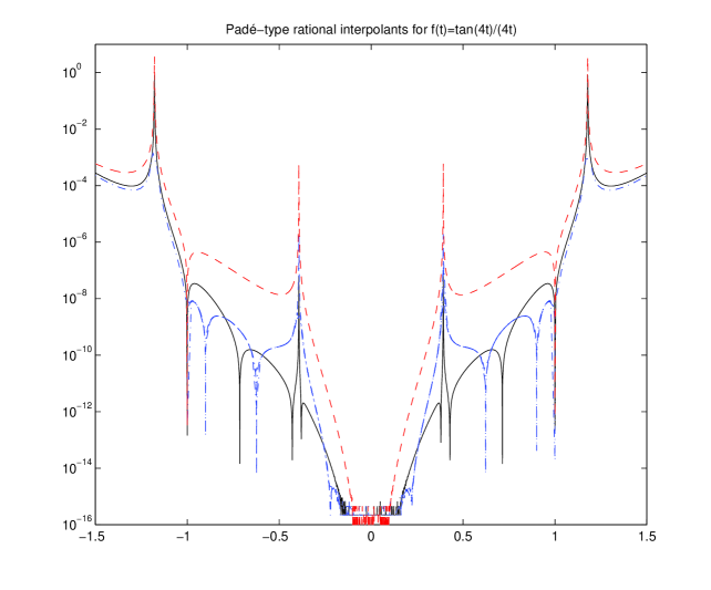
Figure 1: Padé–type rational interpolants with $k=8$ for $\tan(4t)/(4t)$: equidistant points in the interval $[-1,+1]$ (solid), roots of unity (dashed), Chebyshev zeros (dash-dotted).

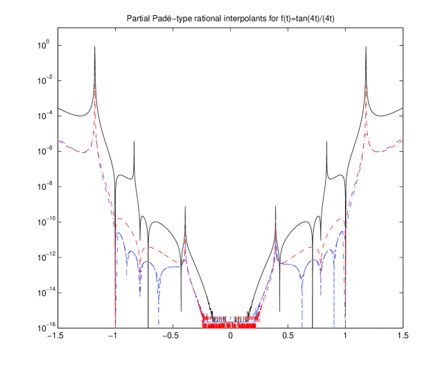
Figure 2: Partial Padé–type rational interpolants with $k=8$ for $\tan(4t)/(4t)$: equidistant points in the interval $[-1,+1]$ (solid), roots of unity (dashed), Chebyshev zeros (dash-dotted).

Example 1: a function with poles

We consider the following function, and its series expansion

$$f(t)=\frac{\tan(\omega t)}{\omega t}=1+\frac{1}{3}\omega^{2}t^{2}+\frac{2}{15}\omega^{4}t^{4}+\frac{17}{315}\omega^{6}t^{6}+\frac{62}{2835}\omega^{8}t^{8}+\cdots$$

This function has poles at odd multiples of $\pi/(2\omega)$, and zeros at odd multiples of $\pi/\omega$, except at 0.

We considered three sets of interpolations points: equidistant points in the interval $[-1,+1]$, the roots of unity, and the zeros of the Chebyshev polynomials of the first kind. The complex choice was discussed in [20]. Let us mention that none of the interpolation points $\tau_{i}$ should be 0, since it is the point where the Padé–type approximants are computed and thus it always appears as an interpolation point.

Padé–type rational interpolants

The errors obtained with the Padé–type rational interpolants are given in Figure 1 for $\omega=4$ and $k=8$. The solid line corresponds to the real interpolation points, while the dashed one refers to the points on the unit circle, and the dash-dotted one to the zeros of the Chebyshev polynomial. The poles of $f$ are, in the interval considered in Figure 1, at the points $\pm 0.39269908\ldots$ and $\pm 1.1780972\ldots$, and the zeros at $\pm 0.78539816\ldots$

Since the poles and the zeros are known, we took $Z_{2}(t)=(t-\pi/4)(t+\pi/4)$ and $P_{2}(t)=(t-\pi/8)(t+\pi/8)$. The errors obtained with the partial Padé–type rational interpolants are displayed in Figure 2. Let us mention that, for some values of $k$, we could observe Froissart’s doublets (nearby poles and zeros) that can be removed by the technique described below (Example 4).

The improvement brought by partially taking into account the knowledge of the poles and of the zeros is clear. Choosing the zeros of the Chebyshev polynomials as the real interpolation points in $[-1,+1]$ does not change much the quality of the results for such small values of $k$.

Padé–type barycentric interpolants

Let us now consider the same example but with the Padé–type barycentric interpolants. The results are given in Figure 3. With the partial Padé–type barycentric interpolants, we obtain the results of Figure 4. In both figures, the solid line corresponds to the real interpolation points, and the dashed one to the interpolation points on the unit circle.

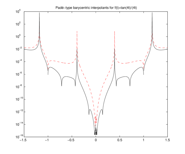
Figure 3: Padé–type barycentric interpolants with $k=8$ for $\tan(4t)/(4t)$: equidistant points in the interval $[-1,+1]$ (solid), roots of unity (dashed).

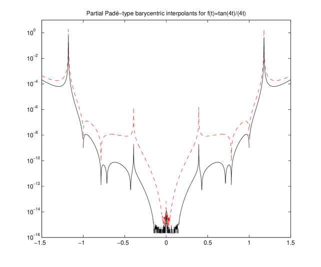
Figure 4: Partial Padé–type barycentric interpolants with $k=8$ for $\tan(4t)/(4t)$: equidistant points in the interval $[-1,+1]$ (solid), roots of unity (dashed).

Let us mention that, with the Shepard’s weights $w_{i}=1/(t-\tau_{i})$ [27], the interpolants have poles around $-0.4$ and $+0.4$.

Example 2: a function with a cut

We consider the series

$$f(t)=\frac{\log(1+t)}{t}=1-\frac{t}{2}+\frac{t^{2}}{3}-\frac{t^{3}}{4}+\cdots$$

which converges in the unit disk and on the unit circle except at the point $-1$ since there is a cut from $-1$ to $-\infty$.

Padé–type rational interpolants

For a Padé–type interpolant of degree 7, we consider equidistant real interpolation points in the interval $[-0.9,+1.2]$. For 7 points (solid line), the system to be solved is square. For 3 points (dashed line) and 14 points (dash–dotted line), the system is solved in the least squares sense as explained above. The results are given in Figure 5. We see that they are quite good even for values of $t$ far outside the convergence interval.

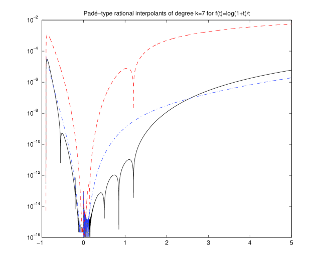
Figure 5: Padé–type rational interpolants with $k=7$ for $\log(1+t)/t$, and 3 (dashed), 7 (solid) and 14 (dash-dotted) interpolation points.

Padé–type barycentric interpolants

The interpolation points $\tau_{i}$ are taken equidistant in $[-0.9,+4]$, and $k=7$. In Figure 6, three types of weights $w_{i}$ are considered: those corresponding to the Padé–type barycentric interpolants are the same as explained above (solid line), the weights $w_{i}=(-1)^{i}$ of Berrut [2] (dashed line), and the weights $w_{i}=1/(t-\tau_{i})$ suggested by Shepard [27] (dash–dotted line), these last two choices ensuring pole–free interpolants on the real line.

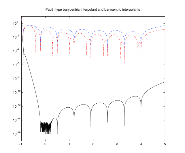
Figure 6: Padé–type barycentric interpolants with $k=7$ for $\log(1+t)/t$ (solid). Barycentric interpolants with Berrut weights (dashed), and Shepard weights (dash-dotted).

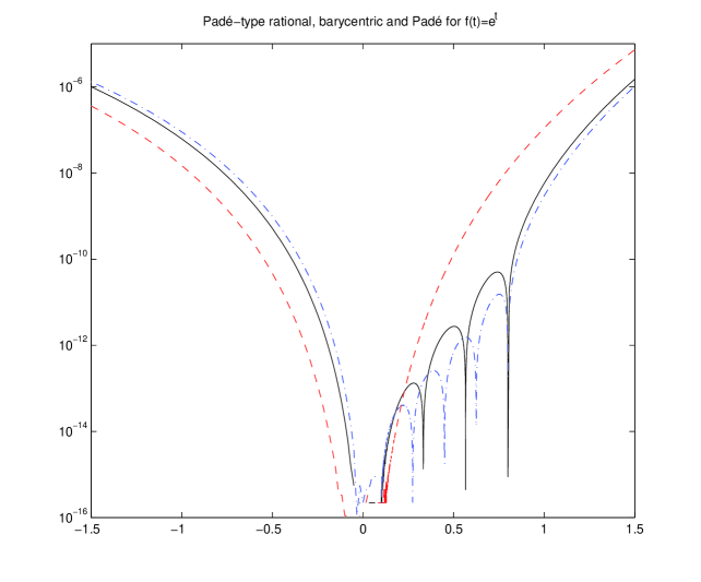
Figure 7: Padé–type rational (solid) and barycentric (dash-dotted) interpolants, and Padé approximant (dashed) for $e^{t}$.

Example 3: a continuous function

We consider the exponential function

$$f(t)=e^{t}=1+\frac{t}{1!}+\frac{t^{2}}{2!}+\cdots$$

Let us now compare, for the degree $k=4$, the Padé–type rational interpolant, the Padé–type barycentric interpolant, and the Padé approximant $[4/4]$ which is given by

$$[4/4]_{f}(t)=(1680+840t+180t^{2}+20t^{3}+t^{4})/(1680-840t+180t^{2}-20t^{3}+t^{4}).$$

Let us remind that $[4/4]_{f}(t)-e^{t}={\cal O}(t^{9})$, and that its construction makes use of the first 8 coefficients of the power series. The results are given in Figure 7, where the solid line represents the error of the Padé–type rational interpolant, the dashed line corresponds to the Padé approximant, and the dash–dotted line to the Padé–type barycentric interpolant.

The interpolation points were chosen equidistant in the interval $[0.1,0.8]$. Notice that, for the interpolants, the error is smaller around the interpolation points, while the errors of the Padé approximant is more symmetric around the origin.

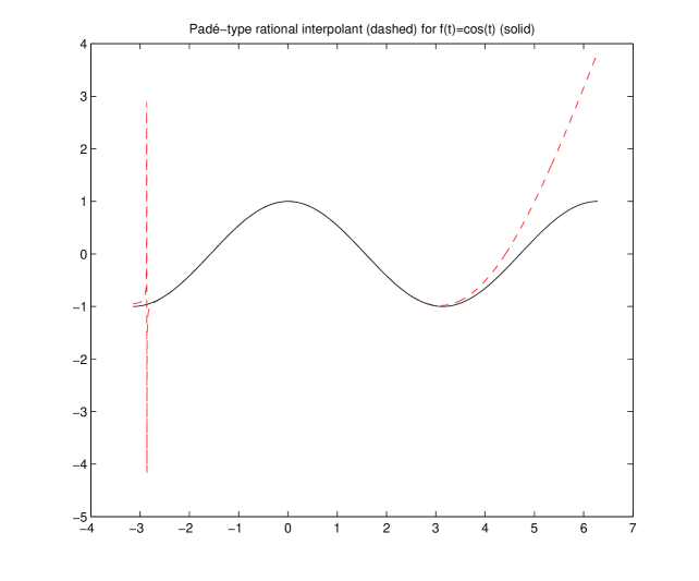
Figure 8: Padé–type rational interpolant (dashed) of the cosine function (solid).

Example 4: spurious pole removal

Let us now give an example showing that the rational interpolant can have poles even if the function is continuous. In fact, it is known [25] that if, after cancelation of common factors between the numerator and the denominator and ordering the interpolation points, two consecutive weights $w_{i}$ and $w_{i+1}$ in the barycentric formula have the same sign, then the reduced interpolant has an odd number of poles in $[\tau_{i},\tau_{i+1})$.

We consider the Padé–type rational interpolant of the cosine function with 5 equidistant interpolation points in the interval $[-\pi/2,+\pi/8]$. As may be seen in Figure 8, the interpolant (dashed line) has one real pole at $t=-2.8636\ldots$ (its other poles are complex). When $t$ goes to infinity, the interpolant tends to $25.269\ldots$

However, the results are quite good (the cosine function is the solid line in Figure 8) from the right of the pole up to almost $\pi$.

It is possible to remove a spurious pole $p$ by forcing the Padé–type interpolant to go through the point $(p,f(p))$. In Figure 9, the first of the equidistant interpolation points is replaced by the pole $p$, a procedure which removes it and leads to a better result (dashed line).

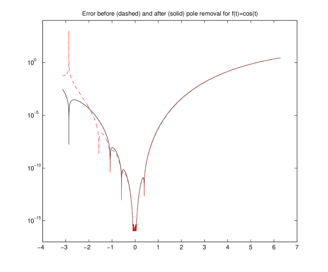
Figure 9: Error before (solid) and after (dashed) the pole removal in the Padé–type rational interpolant for $f(t)=\cos t$.

If the interpolant exhibits several poles, they can be eliminated successively. If a new pole is introduced during the procedure, then it can be removed similarly.

In our case, the location of the pole was directly computed from the coefficients $b_{i}$ of the denominator of the interpolant since they were available. It is also possible to locate approximately a pole when the absolute value of the interpolant becomes larger than a fixed threshold, or when the interpolant has a sudden change of sign, and then to impose it as an interpolation point.

This procedure was tried on the Padé–type barycentric interpolant for $\cos t$ in the same interval as before, but with $k=13$. The interpolant was computed at 500 points in $[-\pi,+2\pi]$. A sudden change of sign was observed in the interval $[5.3010,5.3199]$. We had $R_{13}(5.3010)=15.068$ and $R_{13}(5.3199)=-25.101$. Replacing the first interpolation point $\tau_{0}=-\pi/2$ by $\tau_{0}=5.3050$, the spurious pole was removed, and no other pole appeared.

The advantage of this procedure is that it can also be used for Padé–type barycentric interpolants where the coefficients of the denominator are not explicitly known.

The same techniques can be applied to the case of partial Padé–type rational and barycentric interpolation.

7 Applications

Let us now briefly discuss some possible applications to numerical analysis problems.

7.1 Convergence acceleration

We consider the sequence $(S_{n}=f(\tau_{n}))$ where $(\tau_{n})$ is a sequence of parameters such that $\lim_{n\to\infty}\tau_{n}=\tau_{\infty}\neq 0,\pm\infty$, and where $f$ is a function whose first coefficients of the series expansion around 0 are known. We set $S=\lim_{n\to\infty}S_{n}$.

The convergence of the sequence $(S_{n})$ can be accelerated by computing the Padé–type rational interpolant or the Padé–type barycentric interpolant $R_{k}^{(n)}$ satisfying $R_{k}^{(n)}(\tau_{i})=S_{i}$ for $i=0,\ldots,k-1$ (or $k$ in the second case), and setting $T_{k}^{(n)}=R_{k}^{(n)}(\tau_{\infty})$.This is the essence of an extrapolation method for accelerating the convergence of a sequence [12]. Under certain assumptions, the sequences $(T_{k}^{(n)})$ converge to $S$ faster than $(S_{n})$ either when $k$ is fixed and $n$ goes to infinity, or vice versa.

7.2 Inversion of the Laplace transform

We consider the Laplace transform

$$F(p)=\int_{0}^{\infty}e^{-ps}f(s)\,ds.$$

Assume that $F$ is known at some points $p_{n}$ for $n=0,\ldots,k-1$ (or $k$), and also the first coefficients of its series expansion around 0. $F$ can be approximated by a Padé–type rational interpolant or by a Padé–type barycentric interpolant $R_{k}$, and the interpolant then inverted, thus leading to an approximation of $f$. Let us remark that, since $\lim_{p\to\infty}F(p)=0$, the degree of the numerator of the interpolant must be smaller than the degree of its denominator. The inversion can be performed without decomposing $F$ into its partial fractions by a procedure due to Longman and Sharir [19]. Let $F$ have the form

$$F(p)=A\frac{p^{m}+\alpha_{1}p^{m-1}+\cdots+\alpha_{m}}{p^{n}+\beta_{1}p^{n-1}+\cdots+\beta_{n}},$$

with $m<n$. They showed that

$$f(s)=A\sum_{i=0}^{\infty}\frac{v_{i}}{i!}s^{i}$$

with

$$v_{i}=u_{i+m}+\alpha_{1}u_{i+m-1}+\cdots+\alpha_{m}u_{i},\quad i=0,1,\ldots,$$

where

$$u_{i} = 0,\qquad i=0,\ldots,n-2,$$

$$u_{n-1} = 1,$$

$$u_{i} = -(\beta_{1}u_{i-1}+\cdots+\beta_{n}u_{i-n}),\quad i=n,n+1,\ldots$$

Usually, the series giving $f$ is quickly converging.

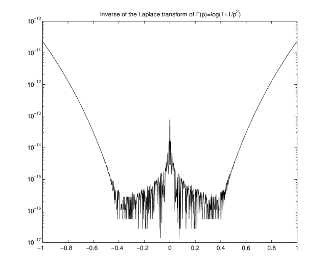
Figure 10: Error for the inversion of the Laplace transform of $F(p)=\log(1+1/p^{2})$.

Let us take the example considered in [12, p. 350]

$$F(p)=\log(1+a^{2}/p^{2}),\qquad f(s)=2(1-\cos as)/s.$$

We make the change of variable $t=a^{2}/p^{2}$, and we set

$$F(p)=G(t)=\log(1+t)=t-\frac{t^{2}}{2}+\frac{t^{3}}{3}-\cdots$$

The Padé–type (rational and barycentric) interpolants will be approximations of $G$. Replacing $t$ by $a^{2}/p^{2}$ in a Padé–type rational interpolant of degree $k$ in $t$ produces an interpolant of degree $2k$ in $p$, and we obtain an approximation of $F$ of the form

$$R_{2k}(p)=\frac{a_{0}p^{2k}+a_{1}a^{2}p^{2k-2}+\cdots+a_{k}a^{2k}}{b_{0}p^{2k}+b_{1}a^{2}p^{2k-2}+\cdots+b_{k}a^{2k}}.$$

Notice that, since $c_{0}=0$ in the series expansion of $G(t)$, the relations (1) lead to $a_{0}=0$, and, thus, $\lim_{p\to\infty}R_{2k}(p)=0$ which is consistent with the asymptotic property of the Laplace transform. Thus, this approximant can be written as

$$R_{2k}(p)=A\frac{p^{2k-2}+\alpha_{2}p^{2k-4}+\cdots+\alpha_{2(k-1)}}{p^{2k}+\beta_{2}p^{2k-2}+\cdots+\beta_{2k}},$$

with $A=a^{2}a_{1}/b_{0}$, $\alpha_{2i}=a^{2i}(a_{i+1}/a_{1})$, for $i=1,\ldots,k-1$, $\beta_{2i}=a^{2i}(b_{i}/b_{0})$, for $i=1,\ldots,k$, the $\alpha$’s and the $\beta$’s with an odd index being zero. We see that the series expansion of $R_{2k}(p)$ only contains even powers of $1/p$ as the series $F(p)$ itself. Inverting $R_{2k}$ by the procedure of Longman and Sharir [19] (after replacing $m$ by $2k-2$ and $n$ by $2k$ in the formulae for the $v_{i}$’s and the $u_{i}$’s), or performing its partial fraction decomposition, gives an approximation of $f$.

For $k=5$, $a=1$, $\tau_{i}=1/p_{i}^{2}$ with $p_{i}=0.1+ih$ for $i=0,\ldots,k-1$, and $h=2/(k-1)$, the Padé–type rational interpolant leads to the results of Figure 10, using 12 terms in the series expansion of $f$. Although $f(0)=0$ and the series expansion by the method of Longman and Sharir is also 0 at $s=0$ (since $v_{0}=0$), there is a loss of accuracy around this point due to the indeterminacy. These results have to be compared with those given in [12, p. 350] which were obtained by constructing a rational interpolant with a numerator of degree 7 and a denominator of degree 8, that is using 16 interpolation points. We see that our Padé–type rational interpolant provides a much better precision. Moreover, the precision can be even improved by taking more terms in the series for $f$ at almost no additional price.

This example could also be treated by making the change of variable $t=a/p$, thus leading to $F(p)=G(t)=\log(1+t^{2})=t^{2}-t^{4}/2+t^{6}/3-\cdots$.

7.3 Piecewise rational interpolation

Our approach can be used for constructing piecewise rational interpolants. Let $a<a^{\prime}\leq 0\leq b^{\prime}<b$. We construct a first Padé–type rational or barycentric interpolant in $[a,a^{\prime}]$, and then a second one in $[b^{\prime},b]$. Due to the Padé–type property of these interpolants and the fact that, for all $i$, $c_{i}=f^{(i)}(0)/i!$, the two interpolants and their first derivatives will have the same values at the point $t=0$. Obviously, by a change of variable, the same construction holds at a point different from the origin, and it can be repeated.

One of the advantages of such a construction is to obtain a good accuracy with a low degree in the interpolants, thus avoiding the usually bad conditioning when using more interpolation points and a rational interpolant with a higher degree.

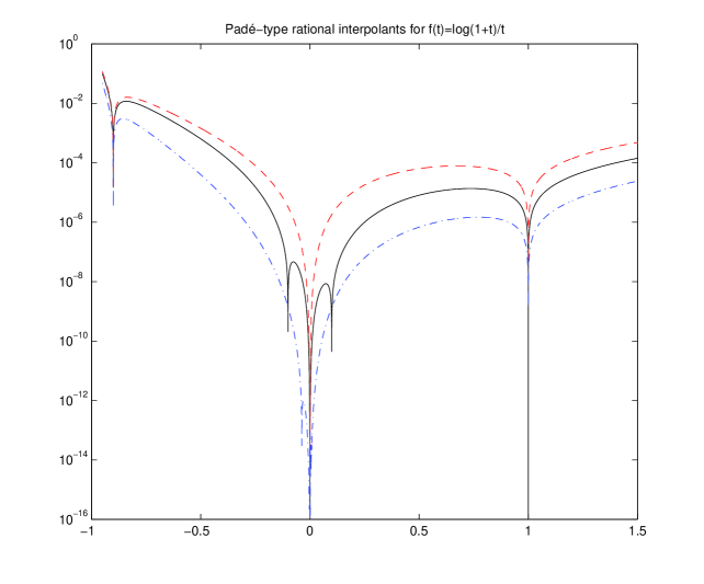
Figure 11: Padé–type rational interpolants for $\log(1+t)/t$: the piecewise case.

We interpolate the function $f(t)=\log(1+t)/t$ on the intervals $[-0.9,-0.1]$ and $[+0.1,+1]$ with $k=2$, which means that the first rational function interpolates $f$ only at the points $-0.9$ and $-0.1$, and the second ones interpolates it at $+0.1$ and $+1$. These two interpolants and their first and second derivatives agree with that of $f$ at $t=0$. The solid line in Figure 11 corresponds to the curve formed by these two Padé–type rational interpolants. The two systems have a condition number of $3.25\times 10^{4}$ and $2.86\times 10^{4}$, respectively. Then, we construct the Padé–type rational interpolant interpolating $f$ at the 4 points $-0.9,-0.1,+0.1$ and $+1$, and with a ${\cal O}(t^{3})$ error at the origin. The system is overdetermined since $l>k$, its condition number is $1.90\times 10^{3}$, and the error is given by the dashed line. Finally, with the same 4 interpolation points, we construct the interpolant of degree $k=3$. The system is also overdetermined, its condition number is $6.37\times 10^{13}$, and we obtain the results given by the dash–dotted line.

8 Conclusions

In this paper, we presented in details the particular case of the general rational Hermite interpolation problem (in rational and barycentric form) where only the values of the function are interpolated at some points, and where the function and its first derivatives agree at the origin. Thus, the interpolants constructed in this way possess a Padé–type property at 0. An expression for the error in the real case is given. The interpolation procedure can be easily modified to introduce a partial knowledge on the poles and the zeros of the function to approximated. We also showed how spurious poles can be eliminated. Numerical examples show the interest of the procedures.

The ideas developed in this paper need additional investigations. An important open problem is to be study the convergence of the interpolants when the degree tends to infinity as done in [16] for Padé–type approximants. In our case, we performed some numerical experiments which show that, in some cases, convergence seems to occur while, in some others, no conclusion could be drawn since, for high degrees, the systems are numerically singular.

Acknowledgment: We would like to thank Jean–Paul Berrut for interesting discussions and comments. This work was partially supported by MIUR, PRIN grant no. 20083KLJEZ-003, and by University of Padova, Project 2010 no. CPDA104492.

References

- [1] G.A. Baker Jr., P.R. Graves–Morris, Padé Approximants, 2nd edition, Cambridge University Press, Cambridge, 1996.
- [2] J.–P. Berrut, Rational functions for guaranteed and experimentally well-conditioned global interpolation, Comput. Math. Appl., 15 (1988) 1–16.
- [3] J.–P. Berrut, R. Baltensperger, H.D. Mittelmann, Recent developments in barycentric rational interpolation, in Trends and Applications in Constructive Approximation, M.G. de Bruin, D.H. Mache, J. Szabados eds., ISNM vol. 151, Birkhäuser Verlag, Basel, 2005, pp. 27–51.
- [4] J.–P. Berrut, H.D. Mittelmann, Lebesgue constant minimizing linear rational interpolation of continuous functions over the interval, Comput. Math. Appl., 33 (1997) 77–86.
- [5] J.–P. Berrut, H.D. Mittelmann, Matrices for the direct determination of the barycentric weights of rational interpolation, J. Comput. Appl. Math., 78 (1997) 355–370.
- [6] C. Brezinski, Rational approximation to formal power series, J. Approx. Theory, 25 (1979) 295–317.
- [7] C. Brezinski, Padé–Type Approximation and General Orthogonal Polynomials, ISNM, vol. 50, Birkhäuser–Verlag, Basel, 1980.
- [8] C. Brezinski, Partial Padé approximation, J. Approx. Theory, 54 (1988) 210–233.
- [9] C. Brezinski, Biorthogonality and its Applications to Numerical Analysis, Marcel Dekker, New York, 1992.
- [10] C. Brezinski, Computational Aspects of Linear Control, Kluwer, Dordrecht, 2002.
- [11] C. Brezinski, Extrapolation algorithms for filtering series of functions, and treating the Gibbs phenomenon, Numer. Algorithms, 36 (2004) 309–329.
- [12] C. Brezinski, M. Redivo–Zaglia, Extrapolation Methods. Theory and Practice, North–Holland, Amsterdam, 1991.
- [13] C. Brezinski, J. Van Iseghem, Padé approximations, in Handbook of Numerical Analysis, vol. III, P.G. Ciarlet and J.L. Lions eds., North–Holland, Amsterdam, 1994, pp. 47–222.
- [14] C. Brezinski, J. Van Iseghem, A taste of Padé approximation, in Acta Numerica 1995, A. Iserles ed., Cambridge University Press, Cambridge, 1995, pp. 53–103.
- [15] A. Cuyt, L. Wuytack, Nonlinear Methods in Numerical Analysis, North–Holland, Amsterdam, 1987.
- [16] M. Eiermann, On the convergence of Padé–type approximants to analytic functions, J. Comput. Appl. Math., 10 (1984) 219–227.
- [17] M.S. Floater, K. Hormann, Barycentric rational interpolation with no poles and high rates of approximation, Numer. Math., 107 (2007) 315–331.
- [18] P.R. Graves–Morris, Efficient reliable rational interpolation, in Padé Approximation and its Applications. Amsterdam 1980, M.G. de Bruin and H. van Rossum eds., LNM vol. 888, Springer–Verlag, Berlin, Heidelberg, New York, 1981, pp. 28–63.
- [19] I. M. Longman, M. Sharir. Laplace transform inversion of rational functions, Geophys. J. R. Astron. Soc., 25 (1971) 299–305.
- [20] P. Gonnet, R. Pachón, L.N. Trefethen, Robust rational interpolation and least–squares, Electron. Trans. Numer. Anal., 38 (2011) 146–167.
- [21] G. Hornecker, Approximations rationnelles voisines de la meilleure approximation au sens de Tchebycheff, C. R. Acad. Sci. Paris, 249 (1959) 939–941.
- [22] G. Hornecker, Détermination des meilleures approximations rationnelles (au sens de Tchebycheff), des fonctions réelles d’une variable sur un segment fini et des bornes d’erreur correspondantes, C. R. Acad. Sci. Paris, 249 (1959) 2265–2267.
- [23] L.M. Milne–Thomson, The Calculus of Finite Differences, The Macmillan Press, London, 1933.
- [24] S. Paszkowski, Approximation uniforme des fonctions continues par les fonctions rationnelles, Zastos. Mat., 6 (1963) 441–458.
- [25] C. Schneider, W. Werner, Some new aspects of rational interpolation, Math. Comput., 47 (1986) 285–299.
- [26] C. Schneider, W. Werner, Hermite interpolation: the barycentric approach, Computing, 46 (1991) 35–51.
- [27] D. Shepard, A two–dimensional interpolation function for irregularly–spaced data, in Proceedings of the 23rd ACM National Conference, ACM Press, New York, 1968, pp. 517- 524.
- [28] J. Van Deun, Eigenvalue problems to compute almost optimal points for rational interpolation with prescribed poles, Numer. Algorithms, 45 (2007) 89–99.
- [29] J. Van Deun, Computing near-best fixed pole rational interpolants, J. Comput. Appl. Math., 235 (2010) 1077 -1084.
- [30] P. Wynn, Transformations to accelerate the convergence of Fourier series, in Gertrude Blanch Anniversary Volume, Wright Patterson Air Force Base, Aerospace Research Laboratories, Office of Aerospace Research, United States Air Force, 1967, pp. 339–379.