Is reduced-density-matrix functional theory a suitable vehicle to import explicit correlations into density-functional calculations?

Abstract

A variational formulation for the calculation of interacting fermion systems based on the density-matrix functional theory is presented. Our formalism provides for a natural integration of explicit many-particle effects into standard density-functional-theory based calculations and it avoids ambiguities of double-counting terms inherent to other approaches. Like the dynamical mean-field theory, we employ a local approximation for explicit correlations. Aiming at the ground state only, trade some of the complexity of Green’s function based many-particle methods against efficiency. Using short Hubbard chains as test systems we demonstrate that the method captures ground state properties, such as left-right-correlation, beyond those accessible by mean-field theories.

I Introduction

One of the most successful theories in solid-state physics is the density-functional theory (DFT) Hohenberg and Kohn (1964); Kohn and Sham (1965). Its present implementations predict properties of materials with an accuracy, which makes it a standard tool for material scientists both in fundamental research and in industry.

One of the major deficiencies of currently available density functionals is the description of materials with strong electron correlations. Strong electron correlations develop when the interaction between the electrons dominates over the kinetic energy. While the kinetic energy favors delocalized electron states and well-defined energy bands in reciprocal space, strong interactions may lead to a complete breakdown of the band picture.

Strongly correlated materials often contain 3d transition-metal elements or rare-earth elements with partially filled f-electron shells. The d- and f-electrons are on the one hand localized core-like states, but, on the other hand, they are located energetically in the region of valence states. Thus, their nature is right at the border between localized and delocalized behavior.

Strong correlations are responsible for a wealth of new properties with potential technological relevance. Among them are heavy-fermion systemsStewart (1984), Mott insulators and the Mott-Hubbard metal-insulator transition (MHMIT)Imada et al. (1998), high-temperature superconductorsDagotto (1994) and the colossal magnetoresistanceSalamon and Jaime (2001). More recently, the vicinity to phase transitions in those systems has opened the field of quantum criticality v. Löhneysen et al. (2007).

It is a fascinating challenge to unravel the underlying mechanisms behind these phenomena and eventually to rationally design applications exploiting them. A theoretical treatment of these systems, however, turns out to be a rather big challenge and has been at the frontier of research in condensed matter physics since nearly half a century.Imada et al. (1998) The use of explicit many-body tools is nearly impossible for complex materials like perovskites. Therefore, the many-body community tries to identify the minimal set of degrees of freedom relevant for the physical properties and sets up a model hamiltonian for these degrees of freedom. The best known of these models is the Hubbard model Hubbard (1963); Kanamori (1963); Gutzwiller (1963), which has been the working horse for correlation effects in transition metal compounds for almost 50 years.

A first attempt to combine DFT with techniques from many-body theory was made with the GW method Aryasetiawan and Gunnarsson (1998), which supplements DFT with certain classes of Feynman diagrams. While the GW scheme was applied to semi-conductors with some success Aryasetiawan and Gunnarsson (1998), it still fails to describe the physics of the MHMIT.

A partial success along this line was achieved by the so-called LDA+U approach, which complements the density functionals by Hartree-Fock type local correlationsAnisimov et al. (1991). Hybrid density functionalsBecke (1993), which replace part of the exchange energy with the exact non-local exchange energy, capture essentially the same physics. These functionals lead to a large improvement of the band gaps, and transition-metal oxides appear correctly as antiferromagnetic charge-transfer insulators, where conventional GGA-type functionals erroneously predict metals or a small d-d band gap.Rollmann et al. (2004) It is, however, important to emphasize that within LDA+U one can only describe materials with ordered ground states satisfactorily, while the MHMIT in the paramagnetic state, as in V₂O₃, cannot be explained with this method.

A quantum leap in the understanding of the MHMIT was achieved by the invention of the dynamical mean-field theory (DMFT) Georges et al. (1996), which provides an efficient and reliable tool to approximately solve the correlation problem for Hubbard type models with local interactions Imada et al. (1998). DMFT keeps the local dynamics intact, which turns out to be essential for the MHMIT. Hence, this theory can actually describe the competition between the Fermi liquid and the interaction driven insulatorGeorges et al. (1996); Pruschke et al. (1995), and also allows for the inclusion of ordered phases beyond standard Hartree theory Obermeier et al. (1997); Zitzler et al. (2002); Pruschke (2005). The price to pay is the neglect of non-local physics and that DMFT fails to capture phenomena like unconventional superconductivity or quantum criticality based on spatial fluctuations v. Löhneysen et al. (2007). Note, however, that these effects can be re-included to a certain extent by extending the original theory Maier et al. (2005)

Rather soon it was realized, that the DMFT can be combined with DFT in a fashion similar to GW.Kotliar and Vollhardt (2004); Kotliar et al. (2006); Held et al. (2006) Indeed, early successes of the method comprise the proper description of spectral properties of $($Sr,Ca$)$VO₃, the MHMIT in V₂O₃, the energetics of the volume collapse in cerium Held et al. (2006), and the lattice properties of plutonium Savrasov et al. (2001), to name a few.

However, as the DMFT is model-hamiltonian based, it requires the definition of a Hubbard model prior to its application. This means, that one needs to extract from DFT (i) the hopping parameters of the Hubbard model and (ii) the local Coulomb parameters. Both are highly ill-defined quantities, because the results strongly depend on the basis set and the sub-manifold of orbitals taken into account. Here, a large effort has been put forward during the past years to define a fairly universal interface between the wave-function based DFT and the Green function based DMFT Anisimov et al. (2005); Lechermann et al. (2006); Jacob et al. (2008); Amadon et al. (2008); Haule et al. (2010).

Besides these technical problems, there are further caveats of the method. Firstly, the DFT does already include certain correlation effects. These have to be “subtracted” from the DFT prior to the calculation of tight-binding and interaction parameters to avoid double-counting in the DMFT calculation. This subtle aspect is one of the most challenging problems in the combination of DFT and DMFT so far, because nobody knows to what extent and in what form in the diagrammatic language correlations effects are included in DFT and how to actually properly remove them Kotliar et al. (2006).

Secondly, within a many-body formulation, the interactions within the subspace of the correlated orbitals will be screened by the other electronic degrees of freedom in the spirit of GW Aryasetiawan et al. (2004). This means, that the actual interactions become retarded. This poses a serious challenge for the computational tools necessary to solve the effective quantum impurity model arising within DMFT.

And last, but not least, the combination of DFT and DMFT cannot be put rigorously on a variational basis. One can, in principle, formulate an extremal principle Anisimov et al. (2005); Kotliar et al. (2006) involving both wave function for DFT and Green functions for DMFT, but the actual connection between these two worlds and a proper subtraction of double counting terms is not obvious.

Therefore, a method, which is fully variational and allows to include both correlations as they are described by conventional density functionals and a reasonable and controlled approximation for strong local correlations, is clearly desirable. The aim of this paper is to propose such an approach. The guiding idea is to reformulate the variational problem in terms of the one-particle density matrix, which is known as reduced-density-matrix functional theory (rDMFT). This problem is of the same complexity as a complete many-particle calculation. Therefore we introduce a local approximation to avoid the dimensional bottleneck.

The origin of rDMFT goes back to Gilbert’s theoremGilbert (1975). Gilbert proved that every ground-state observable can be written as a functional of the one-particle density matrix. Analogously to the development in the field of density-functional theory, research is directed towards the formulation of approximate density-matrix functionals. Most applications use a variation of Müller’s functionalMüller (1984); Goedecker and Umrigar (1998); Csanyi and Arias (2000); Buijse and Baerends (2002); Gritsenko et al. (2005); Sharma et al. (2008). Recent functionals have been able to describe the Mott band gap of transition metal oxides within a non-magnetic descriptionSharma et al. (2008), while density functionals tend to form antiferromagnets instead. This problem is related to the broken-symmetry states of DFT.

In this paper, we explore the main principles of the method. We do not yet approach the question on how to exploit the local nature of the interaction in the Anderson impurity models.

The paper is organized as follows. In the following section II, we present the formulation of the theory in detail. In section III, we sketch the evaluation of the reduced-density-matrix functional using a dynamical optimization similar to the Car-Parrinello methodCar and Parrinello (1985). The workings of our theory will be explored in section IV, where its results for short Hubbard chains are compared with rigorous many-particle calculations.

II Theoretical foundations

II.1 Notation

While our goal is to incorporate many-particle effects into a general electronic structure method such as the projector augmented-wave (PAW) method methodBlöchl (1994), the first step will be to map the electronic structure onto a basisset of local spin orbitals $\chi_{\alpha}(\vec{r},\sigma)=\langle\vec{r},\sigma|\chi_{\alpha}\rangle$. The spin coordinate $\sigma\in\{\uparrow,\downarrow\}$ can assume the values spin-up and spin-down. Each orbital is a two-component spinor, even though we may choose the orbitals such that they only have one non-zero spin component.

In order to decompose an arbitrary one-particle wave function $|\psi\rangle$ into the contribution of the orbitals $|\chi_{\alpha}\rangle$ according to

$$|\psi\rangle=\sum_{\alpha}|\chi_{\alpha}\rangle\langle\pi_{\alpha}|\psi\rangle\,,$$ (1)

we introduce so-called projector states $|\pi_{\alpha}\rangle$. The projector states $\pi_{\alpha}(\vec{r},\sigma)=\langle\vec{r},\sigma|\pi_{\alpha}\rangle$ obey the bi-orthogonality condition

$$\langle\pi_{\alpha}|\chi_{\beta}\rangle=\delta_{\alpha,\beta}\,.$$ (2)

The identity Eq. 1 is valid whenever the wave function can be expanded completely into the orbital set. For a complete orthonormal basisset of local orbitals, the projector states can also be chosen identical to the local orbitals. However, in the most general form, the projector functions differ from the orbitals.

The projector states $|\pi_{\alpha}\rangle$ are conceptually related to the projector functions of the PAW methodBlöchl (1994). They differ from those used for the augmentation, because they provide the amplitudes of the local orbitals instead of partial waves amplitudes provided by the latter. However, in the PAW method the projector states $|\pi_{\alpha}\rangle$ for the local orbitals are naturally constructed as superposition of the projector states for the partial waves.

The creation and annihilation operators in terms of local orbitals can be expressed by the field operators $\hat{\psi}(\vec{r},\sigma)$ and $\hat{\psi}^{\dagger}(\vec{r},\sigma)$ via

$$\hat{c}^{\dagger}_{\alpha} = \sum_{\sigma}\int d^{3}r\;\hat{\psi}^{\dagger}(\vec{r},\sigma)\pi_{\alpha}(\vec{r},\sigma)$$ (3)

$$\hat{c}_{\alpha} = \sum_{\sigma}\int d^{3}r\;\pi^{*}_{\alpha}(\vec{r},\sigma)\hat{\psi}(\vec{r},\sigma)\,.$$ (4)

The back transform is

$$\hat{\psi}^{\dagger}(\vec{r},\sigma) = \sum_{\alpha}\chi^{*}_{\alpha}(\vec{r},\sigma)\hat{c}^{\dagger}_{\alpha}$$ (5)

$$\hat{\psi}(\vec{r},\sigma) = \sum_{\alpha}\hat{c}_{\alpha}\chi_{\alpha}(\vec{r},\sigma)\,.$$ (6)

Creation and annihilation operators obey the anti-commutator relation

$$\left[\hat{c}^{\dagger}_{\alpha},\hat{c}_{\beta}\right]_{+} = \langle\pi_{\alpha}|\pi_{\beta}\rangle$$ (7)

$$\left[\hat{c}^{\dagger}_{\alpha},\hat{c}^{\dagger}_{\beta}\right]_{+} = 0$$ (8)

$$\left[\hat{c}_{\alpha},\hat{c}_{\beta}\right]_{+} = 0\,.$$ (9)

Note, that the anti-commutator between creators and annihilators, i.e. the overlap between projector states, is not necessarily equal to $\delta_{i,j}$. This is due to our generalization to non-orthonormal local orbitals.

The Hamilton operator is given by

$$\hat{H}=\hat{h}+\hat{W}\,,$$ (10)

where $\hat{h}$ is the one-particle part of the Hamilton operator, containing kinetic energy and external potential. $\hat{W}$ is the Coulomb repulsion between the electrons.

The non-interacting Hamiltonian

$$\hat{h}=\sum_{\alpha,\beta}h_{\alpha,\beta}\hat{c}^{\dagger}_{\alpha}\hat{c}_{\beta}$$ (11)

has the matrix elements

$$h_{\alpha,\beta}=\langle\chi_{\alpha}|\frac{\hat{p}^{2}}{2m_{e}}+\hat{V}_{ext}|\chi_{\beta}\rangle\,.$$ (12)

The interaction energy has the form

$$\hat{W}=\frac{1}{2}\sum_{\alpha,\beta,\gamma,\delta}W_{\alpha,\beta,\gamma,\delta}\hat{c}^{\dagger}_{\alpha}\hat{c}^{\dagger}_{\beta}\hat{c}_{\delta}\hat{c}_{\gamma}$$ (13)

with the matrix elements

$$W_{\alpha,\beta,\gamma,\delta} = \sum_{\sigma,\sigma^{\prime}}\int d^{3}r\int d^{3}r^{\prime}\;$$ (14)

$$\times \frac{e^{2}\chi^{*}_{\alpha}(\vec{r},\sigma)\chi^{*}_{\beta}(\vec{r^{\prime}},\sigma^{\prime})\chi_{\gamma}(\vec{r},\sigma)\chi_{\delta}(\vec{r^{\prime}},\sigma^{\prime})}{4\pi\epsilon_{0}|\vec{r}-\vec{r^{\prime}}|}\,.$$

Note the order of the indices of $W_{\alpha,\beta,\gamma,\delta}$ in Eqs. 13 and 14.

II.2 Reduced-density-matrix-functional theory

As shown by GilbertGilbert (1975), every ground-state property of an electron gas can be expressed as functional of a one-particle reduced density matrix. Let us review the basis of the theory:

The ground-state energy for a given external potential can be written as

$$E(\mathbf{h})=\min_{|\Phi\rangle,\mathcal{E}}\Bigl{(} \langle\Phi|\sum_{\alpha,\beta}h_{\alpha,\beta}\hat{c}^{\dagger}_{\alpha}\hat{c}_{\beta}+\hat{W}|\Phi\rangle$$ (15)

$$-\;\mathcal{E}\left(\langle\Phi|\Phi\rangle-1\right)\Bigr{)}\,.$$

The minimization is performed over all fermionic many-particle wave functions $|\Phi\rangle$. $\mathcal{E}$ is the Lagrange multiplier for the normalization constraint of the wave function. The particle number is not restricted and the Fermi level is placed at the energy zero: that is, we implicitly employ a grand-canonical description for the electrons: Electrons are taken from some vacuum level that defines our energy zero and added to the system as long as this addition lowers the total energy.

Let us perform a Legendre transform of the total energy, Eq. 15, with respect to the one-particle Hamiltonian $\mathbf{h}$.

$$F^{\hat{W}}({\bm{\rho}}) = \min_{{\mathbf{h}}}\left[E({\mathbf{h}})-\mathrm{Tr}({\mathbf{h}\bm{\rho}})\right]\,.$$ (16)

The minimum condition of Eq. 16 with respect to $\mathbf{h}$,

$$\rho_{\alpha,\beta}(\mathbf{h}) = \frac{\partial E}{\partial{h}_{\beta,\alpha}}=\langle\Phi|\hat{c}^{\dagger}_{\beta}\hat{c}_{\alpha}|\Phi\rangle\;,$$ (17)

identifies the conjugate variable $\bm{\rho}$ with the one-particle reduced density matrix of the ground state $|\Phi\rangle$ of the Hamiltonian $\hat{h}+\hat{W}$.

The result of the Legendre transform is the reduced-density-matrix functional

$$F^{\hat{W}}({\bm{\rho}})=\min_{|\Phi\rangle,\mathbf{h},\mathcal{E}}\Bigl{[} \langle\Phi|\hat{W}|\Phi\rangle+\sum_{\alpha,\beta}{h}_{\alpha,\beta}\left(\langle\Phi|\hat{c}^{\dagger}_{\alpha}\hat{c}_{\beta}|\Phi\rangle-\rho_{\beta,\alpha}\right)$$ (18)

$$-\;\mathcal{E}\left(\langle\Phi|\Phi\rangle-1\right)\Bigr{]}\,.$$

The reduced-density-matrix functional $F^{\hat{W}}[\bm{\rho}]$ is universal in the sense that it is an intrinsic property of the interacting electron gas and that it is independent of the external potential. We introduced the interaction $\hat{W}$ as superscript in the notation for the reduced-density-matrix functional because we will use different interactions in the course of this paper.

The one-particle Hamiltonian $\mathbf{h}$ required in Eq. 16 to produce a specified density matrix $\bm{\rho}$ is obtained, up to the different sign, as derivative of the density-matrix functional with respect to the density matrix, namely as

$${h}_{\alpha,\beta}(\bm{\rho})=-\frac{\partial F^{\hat{W}}}{\partial\rho_{\beta,\alpha}}\,.$$ (19)

The range of allowed arguments $\bm{\rho}$ for the universal functional is only a subset of all hermitian matrices in the one-particle Hilbert space. The range is limited to the matrices that can be constructed by Eq. 17 with any fermionic many-particle state $|\Phi\rangle$ from the Fock space. Matrices of this form are called N-representable

According to a theorem due to ColemanColeman (1963), the eigenvalues of all N-representable matrices lie between zero and one and all matrices with eigenvalues between zero and one are N-representable.

The eigenstates $|\psi_{n}\rangle$ of the one-particle reduced density matrix are called natural orbitalsLöwdin (1955) and the eigenvalues $f_{n}$ are their occupations. The one-particle density matrix expressed in terms of natural orbitals and occupations is given by

$$\rho_{\alpha,\beta}=\sum_{n}\langle\pi_{\alpha}|\psi_{n}\rangle f_{n}\langle\psi_{n}|\pi_{\beta}\rangle\,.$$ (20)

Hence, the total energy can be expressed by a Legendre back-transform as

$$E(\mathbf{h})=\min_{\{|\psi_{n}\rangle,x_{n},\Lambda_{m,n}\}}\Bigl{[} F^{\hat{W}}\left(\left\{\sum_{n}\langle\pi_{\alpha}|\psi_{n}\rangle f(x_{n})\langle\psi_{n}|\pi_{\beta}\rangle\right\}\right)$$ (21)

$$+\sum_{n,\alpha,\beta}\langle\pi_{\alpha}|\psi_{n}\rangle f(x_{n})\langle\psi_{n}|\pi_{\beta}\rangle{h}_{n,m}$$

$$-\sum_{n,m}\Lambda_{n,m}\left(\langle\psi_{n}|\psi_{m}\rangle-\delta_{m,n}\right)\Bigr{]}\,.$$

In order to respect the limited range of values for the occupations we introduce the transformation $f(x)=\sin^{2}(\frac{\pi}{2}x)$ from an unrestricted real variable $x$ to the interval $[0,1]$. The $\Lambda_{n,m}$ are the Lagrange multipliers for the orthonormality constraint of the natural orbitals.

Starting from the basic formulation of reduced-density-matrix-functional theory, the usual route taken is to find and explore approximate but analytic expressions for the density-matrix functional. We follow a different route, namely to determine the functional on the fly using the explicit constrained-search method of LevyLevy (1979).

II.3 Local approximation

Up to now, the formulation has been exact. However, the evaluation of the density-matrix functional using the constrained search algorithmLevy (1979) requires the solution of a full many-particle problem. Because the many-particle Hilbert space grows exponentially with system size, we introduce approximations that avoid this dimensional bottleneck.

To this end, we introduce clusters $\mathcal{C}_{R}$ of orbitals for which the correlations will be treated explicitly. Such a cluster may include all orbitals from the d- or f-electron shell of an atom; alternatively, it may include all orbitals centered on a single atom, or it may include all or a certain subset of orbitals from several atoms. In analogy to the Anderson impurity model, we will refer to these clusters in the following as ”impurities”.

Besides the full interaction of Eq. 13, we introduce a local interaction $\hat{W}_{\text{loc}}$. Two electrons interact with the local interaction only if both reside on the same impurity, i.e. in the same cluster $\mathcal{C}_{R}$ of correlated orbitals.

$$\hat{W}_{\text{loc}} = \sum\limits_{R}\hat{W}_{R}$$ (22)

$$\hat{W}_{R} := \frac{1}{2}\sum_{\alpha,\beta,\gamma,\delta\in\mathcal{C}_{R}}W_{\alpha,\beta,\gamma,\delta}\;\hat{c}^{\dagger}_{\alpha}\hat{c}^{\dagger}_{\beta}\hat{c}_{\delta}\hat{c}_{\gamma}\,.$$ (23)

Such an interaction is well-known in model-based studies of interaction effects. For example, the Hubbard model uses an interaction of this form.Hubbard (1963); Gutzwiller (1963); Kanamori (1963)

In order to establish the link between DFT and DMFT, let us also introduce an approximate density-matrix-functional $F^{\hat{W}}_{DFT}[\rho]$ calculated from a density functional as

$$F^{\hat{W}}_{DFT}[\bm{\rho}]:=\frac{1}{2}\int d^{3}r\int d^{3}r^{\prime}\;\frac{e^{2}n(\vec{r})n(\vec{r^{\prime}})}{4\pi\epsilon_{0}|\vec{r}-\vec{r^{\prime}}|}+E_{xc}[n(\vec{r})]\,,$$ (24)

where $n(\vec{r}):=\sum_{\alpha,\beta}\rho_{\alpha,\beta}\chi^{*}_{\beta}(\vec{r})\chi_{\alpha}(\vec{r})$ is the electron density.

With the approximate functional from Eq. 24, the density-matrix functional with the full interaction can be written in the form $F^{\hat{W}}=F^{\hat{W}}_{DFT}+(F^{\hat{W}}-F^{\hat{W}}_{DFT})$, i.e. as DFT plus a correction describing many-particle effects explicitly. Irrespective of the choice of the density functional in Eq. 24, this form of the functional is exact, because it simply adds and subtracts the same term to and from the full functional $F^{\hat{W}}$.

The first approximation of our theory is to replace the interaction in the correction term with the sum of local interactions

$$F^{\hat{W}}\approx F_{DFT}^{\hat{W}}+\left(F^{\sum_{R}\hat{W}_{R}}-F_{DFT}^{\sum_{R}\hat{W}_{R}}\right)\,.$$ (25)

On this level, the theory describes interactions on the impurities with the full functional, while the non-local parts of the Coulomb interaction are captured on the DFT level.

The second approximation of our theory is to replace the correction term in Eq. 25 by a sum of local correction terms

$$F^{\hat{W}}\approx F_{DFT}^{\hat{W}}+\sum_{R}\left(F^{\hat{W}_{R}}-F_{DFT}^{\hat{W}_{R}}\right)\,.$$ (26)

In this approximation, the environment of each cluster is replaced by a non-interacting electron gas. Each term $F^{\hat{W}_{R}}$ has precisely the structure of a so-called multi-orbital single-impurity Anderson model.Anderson (1961)

For the sake of completeness, let us quote the error term for the approximation of Eqs. 25 and 26,

$$\Delta F^{\hat{W}} = \left(F^{\hat{W}}-\sum_{R}F^{\hat{W}_{R}}\right)$$ (27)

$$-\left(F_{DFT}^{\hat{W}}-\sum_{R}F_{DFT}^{\hat{W}_{R}}\right)\,.$$

With Eq. 26 we obtain, after including the particle-number constraint, the following expression for the total energy.

$$\bar{E}[\hat{V}_{ext},N] = \min_{\{\psi_{n},x_{n}\}}\Biggl{\{}\sum_{n}f(x_{n})\langle\psi_{n}|\frac{\hat{p}^{2}}{2m_{e}}+\hat{V}_{ext}|\psi_{n}\rangle+\frac{1}{2}\int d^{3}r\,d^{3}r^{\prime}\;\frac{e^{2}n(\vec{r})n(\vec{r^{\prime}})}{4\pi\epsilon_{0}|\vec{r}-\vec{r^{\prime}}|}+E_{xc}[n(\vec{r})]$$ (28)

$$+\sum_{R}\Bigl{\{}F^{\hat{W}_{R}}\biggl{[}\langle\pi_{\alpha}|\psi_{n}\rangle f(x_{n})\langle\psi_{n}|\pi_{\beta}\rangle\biggr{]}-\frac{1}{2}\int d^{3}r\,d^{3}r^{\prime}\;\frac{e^{2}n_{R}^{\chi}(\vec{r})n_{R}^{\chi}(\vec{r^{\prime}})}{4\pi\epsilon_{0}|\vec{r}-\vec{r^{\prime}}|}-E^{\hat{W}_{R}}_{xc}[n^{\chi}(\vec{r})]\Bigr{\}}$$

$$-\sum_{n,m}\Lambda_{n,m}\Bigl{(}\langle\psi_{m}|\psi_{n}\rangle-\delta_{n,m}\Bigr{)}-\mu\Bigl{(}\sum_{n}f(x_{n})-N\Bigr{)}\Biggr{\}}\,,$$

where, with $f_{n}=f(x_{n})$,

$$n(\vec{r}) = \sum_{\sigma}\sum_{n}\langle\vec{r},\sigma|\psi_{n}\rangle f_{n}\langle\psi_{n}|\vec{r},\sigma\rangle\;,$$ (29)

$$n^{\chi}(\vec{r}) = \sum_{\sigma}\sum_{\alpha,\beta}\langle\vec{r},\sigma|\chi_{\alpha}\rangle$$ (30)

$$\times\sum_{n}\langle\pi_{\alpha}|\psi_{n}\rangle f_{n}\langle\psi_{n}|\pi_{\beta}\rangle\langle\chi_{\beta}|\vec{r},\sigma\rangle\;,$$

and

$$n^{\chi}_{R}(\vec{r}) = \sum_{\sigma}\sum_{\alpha,\beta\in\mathcal{C}_{R}}\langle\vec{r},\sigma|\chi_{\alpha}\rangle$$ (31)

$$\times\sum_{n}\langle\pi_{\alpha}|\psi_{n}\rangle f_{n}\langle\psi_{n}|\pi_{\beta}\rangle\langle\chi_{\beta}|\vec{r},\sigma\rangle\,.$$

For the sake of simplicity, we write the expression for density functionals and not for spin-density functionals. The generalization is straightforward.

The second line in Eq. 28 can be considered as a correlation correction to the density functional: In the absence of the correlation correction, the theory recovers the conventional expression of density-functional theory.

II.4 Exchange-correlation with local interaction

Finding an expression of the exchange-correlation functional for the interaction is not straightforward.

The exchange-correlation energy can be expressed by the interaction-strength averaged hole functionHarris and Jones (1974) $h_{\lambda}(\vec{r},\vec{r^{\prime}})$ as

$$E_{xc}[n]=\int d^{3}r\;n(\vec{r})\left[\int_{0}^{1}d\lambda\;\frac{1}{2}\int d^{3}r^{\prime}\;\frac{e^{2}h_{\lambda}(\vec{r},\vec{r^{\prime}})}{4\pi\epsilon_{0}|\vec{r}-\vec{r^{\prime}}|}\right]\;.$$ (32)

The hole function is defined via the two-particle density $n^{(2)}_{\lambda}(\vec{r},\vec{r^{\prime}})$ of the ground state for a given density $n(\vec{r})$ or spin density $n_{\sigma,\sigma^{\prime}}(\vec{r})$ as

$$h_{\lambda}(\vec{r},\vec{r^{\prime}})=\frac{1}{n(\vec{r})}\left[n^{(2)}_{\lambda}(\vec{r},\vec{r^{\prime}})-n(\vec{r})n(\vec{r^{\prime}})\right]\;.$$ (33)

The parameter $\lambda$ scales the interaction $\hat{W}$. The corresponding hole function is obtained from the wave function for this scaled interaction. The $\lambda$-average accounts for the difference of the kinetic energy between the interacting and the non-interacting electron gas.

Because the restricted interaction $\hat{W}_{R}$ is nonlocal in the coordinates of each particle, it needs to be modified before it can be used in a density functional. We propose to use the following model for the local interaction

$$v^{\hat{W}_{R}}(\vec{r},\vec{r^{\prime}})=\frac{n^{\chi}_{R}(\vec{r})}{n^{\chi}(\vec{r})}\frac{e^{2}}{4\pi\epsilon_{0}|\vec{r}-\vec{r^{\prime}}|}\frac{n^{\chi}_{R}(\vec{r^{\prime}})}{n^{\chi}(\vec{r^{\prime}})}\,,$$ (34)

where $n_{R}^{\chi}(\vec{r})$ and $n^{\chi}(\vec{r})$ are defined by Eqs. 30 and 31. This choice for the interaction is consistent with the expression for the Hartree energy. It can systematically be extended to the full exchange correlation energy by including the remaining pair terms.

If we use the model for the restricted interaction from Eq. 34 in Eq. 32, we obtain

$$E^{\hat{W}_{R}}_{xc}=\int d^{3}r\;n^{\chi}_{R}(\vec{r})\left[\frac{1}{2}\int d^{3}r^{\prime}\;\frac{e^{2}h(\vec{r},\vec{r^{\prime}})}{4\pi\epsilon_{0}|\vec{r}-\vec{r^{\prime}}|}\frac{n^{\chi}_{R}(\vec{r^{\prime}})}{n^{\chi}(\vec{r^{\prime}})}\right]\,.$$ (35)

Here, the $\lambda$-averaged hole function is used. Hole functions for some of the commonly used density functionals have been developedBahmann and Ernzerhof (2008); Perdew et al. (1996).

Eq. 35 reflects that only electrons on the same impurity interact with each other. Our approximation assumes that the exchange-correlation hole of the Anderson impurity model is identical to that of the fully interacting system. This is strictly valid for the exchange part, while it is an approximation for the correlation contribution.

If the hole function is not available, the most simple approximation is

$$E_{xc}^{\hat{W}_{R}}=\int d^{3}r\;n^{\chi}_{R}(\vec{r})\epsilon_{xc}[n^{\chi}_{\sigma,\sigma^{\prime}}(\vec{r})]\frac{n^{\chi}_{R}(\vec{r})}{n^{\chi}(\vec{r})}\,,$$ (36)

where $\epsilon_{xc}$ is the exchange correlation energy per electron.

II.5 Coulomb matrix elements

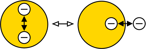
Figure 1: Scheme to demonstrate the case where an electron leaves a correlated region. In the local approximation the interaction with the electron remaining on the correlated cluster is completely removed, explaining the need for renormalizing the Coulomb interaction.(Color online)

One of the important ingredients to our theory is the Coulomb tensor (23) projected onto the impurity orbitals. The first idea is to calculate this tensor using the local orbitals $|\chi_{\alpha}\rangle$ with the bare Coulomb interaction.

However, as in other local approximations, such an approach would result in too large Coulomb parameters for the reason schematically depicted in Fig. 1: If an electron leaves a correlated orbital, it is likely to be located nearby, so that only a portion of the interaction is lost. In the local approximation the Coulomb interaction is completely removed for a particle leaving the correlated impurity. Thus the energy required to add or remove an electron from the impurity is overestimated in the local approximation, respectively charge fluctuations are artificially suppressed. Therefore, our method will require an appropriate renormalization of the local U-tensor to account for those screening channels.

There are several possible approaches to obtain this effect. One can in principle enlarge the impurity and include more extended orbitals in the correlated cluster. This will lead at least partially to the desired renormalization: The screening is taken over by the extended orbitals. Another route, which has proven to be more efficient, is to perform additional calculations using constrained DFT Dederichs et al. (1984), which will also provide an estimate of the renormalization due to screening from other orbitals.

II.6 Extension to ensemble density-matrix functional theory

The formulation of the density-matrix-functional theory used so far is based on pure states, that, however, are not necessarily eigenstates of the particle-number operator. Usually, density-matrix-functional theory is formulated for ensembles of many-particle states. The generalization to ensemble rDMFT is straightforward. A density-matrix-functional for an ensemble of many-particle states has the form

$$F^{\hat{W}}({\bm{\rho}}) = \min_{\{|\Phi_{i}\rangle,P_{i}\}}\Bigl{[}\sum_{i}P_{i}\langle\Phi_{i}|\hat{W}|\Phi_{i}\rangle$$

$$+ \sum_{\alpha,\beta}{h}_{\alpha,\beta}\left(\sum_{i}P_{i}\langle\Phi_{i}|\hat{c}^{\dagger}_{\alpha}\hat{c}_{\beta}|\Phi_{i}\rangle-\rho_{\beta,\alpha}\right)$$

$$- \sum_{i,j}\Lambda_{i,j}\left(\langle\Phi_{i}|\Phi_{j}\rangle-\delta_{i,j}\right)+\lambda\biggl{(}\sum_{i}P_{i}-1)\Bigr{]}\,,$$

where $P_{i}$ are probabilities for the many-particle states $|\Phi_{i}\rangle$. In order to ensure that the probabilities fall between zero and one, we represent them as square $P_{i}=X_{i}^{2}$ of a real number $X_{i}$.

Formally, the theory can be extended to finite temperatures by adding an additional entropy term $-ST=k_{B}T\sum_{i}P_{i}\ln(P_{i})$, that represents a heat bath, to the density matrix functional.

III Evaluation of the density-matrix functional

The reduced-density-matrix functional $F^{\hat{W}_{R}}$ in Eq. 28 is determined directly using the constrained-search formalism of LevyLevy (1979). The details of the methodology will be described elsewhere.

In order to evaluate the density-matrix functional, we translate the fictitious Lagrangian methodology of Car and Parrinello for ab-initio molecular dynamicsCar and Parrinello (1985) to many-particle wave functions $|\Phi\rangle$.

The problem of ab-initio molecular dynamics and of a many-particle problem are related, as far as they are applied to the search for ground states: in both cases one has to determine one or a few of the lowest states of a highly-dimensional Hamiltonian. Furthermore, the fictitious Lagrangian formalism lends itself to the search of a minimum under constraints. In the Car-Parrinello methodCar and Parrinello (1985), the constraints are the orthonormality constraints for the Kohn-Sham wave functions. In our case it is the norm and the requirement that the wave function produces a specified reduced one-particle density matrix.

We start from a fictitious Lagrangian defined as

$$\mathcal{L}(|\Phi\rangle,|\dot{\Phi}\rangle) = \langle\dot{\Phi}|m_{\Phi}|\dot{\Phi}\rangle-\langle\Phi|\hat{W}|\Phi\rangle$$ (38)

$$- \sum_{\alpha,\beta}{h}_{\alpha,\beta}\Bigl{(}\langle\Phi|\hat{c}^{\dagger}_{\alpha}\hat{c}_{\beta}|\Phi\rangle-\rho_{\beta,\alpha}\Bigr{)}$$

$$+ E\Bigl{(}\langle\Phi|\Phi\rangle-1\Bigr{)}\,.$$

In practice, each many-particle wave function is represented by a coefficient array of the Slater determinants.

Including a friction term, the equation of motion has the form

$$m_{\Phi}|\ddot{\Phi}\rangle = -(\sum_{\alpha,\beta}{h}_{\alpha,\beta}\hat{c}^{\dagger}_{\alpha}\hat{c}_{\beta}+\hat{W}-E)|\Phi\rangle-|\dot{\Phi}\rangle\kappa\,.$$ (39)

This equation of motion is discretized using the Verlet algorithmVerlet (1967), and the constraints are taken into account using the method of Ryckaert et al.Ryckaert et al. (1977).

The Car-Parrinello method is not only used to optimize the many-particle wave function for each Anderson impurity model. It is also used more conventionally to optimize dynamically the natural orbitals and occupations in the “outer loop”. This is analogous to the conventional Car-Parrinello method, which optimizes the Kohn-Sham wave functions. Both, natural orbitals and Kohn-Sham wave functions are single-particle wave functions.

IV Model calculations

In order to explore the workings of the formalism described in the previous sections, we performed calculations on model systems that allow comparison to exact results.

The model systems are Hubbard chains with $N_{s}=2$, $N_{s}=4$, and $N_{s}=6$ sites. Their Hamiltonian is

$$\hat{H} = \hat{T}+\sum_{R=1}^{N_{s}}\hat{W}_{R}\,,$$ (40)

where $\hat{T}$ describes the non-interacting part of the Hamiltonian

$$\hat{T}=-t\sum_{R=1}^{N_{s}-1}\sum_{\sigma\in\{\uparrow,\downarrow\}}\biggl{(}\hat{c}_{R,\sigma}^{\dagger}\hat{c}_{R+1,\sigma}+\hat{c}_{R+1,\sigma}^{\dagger}\hat{c}_{R,\sigma}\biggr{)}\,,$$ (41)

and $\hat{W}_{R}$ is the interaction on a the $R$-th site

$$\hat{W}_{R}=U\hat{n}_{R,\uparrow}\hat{n}_{R,\downarrow}\,.$$ (42)

$t$ is the hopping parameter and $U$ is the Coulomb parameter. $\hat{n}_{R,\sigma}=\hat{c}^{\dagger}_{R,\sigma}\hat{c}_{R,\sigma}$ is the particle-number operator for the specified orbital.

We adapted Eq. 28 to the Hubbard chain by ignoring Hartree and exchange energy terms. They cancel exactly on this level of the theory.

$$\bar{E}(N) = \min_{\{|\psi_{n}\rangle,x_{n}\}}\biggl{\{}\sum_{n}f(x_{n})\langle\psi_{n}|\hat{T}|\psi_{n}\rangle+\sum_{R}F^{\hat{W}_{R}}(\{\rho_{\alpha,\beta}\})$$ (43)

$$-\sum_{n,m}\Lambda_{n,m}\biggl{(}\langle\psi_{m}|\psi_{n}\rangle-\delta_{m,n}\biggr{)}-\mu\biggl{(}\sum_{n}f(x_{n})-N\biggr{)}\,,$$

where the $f(x_{n})$ are the occupations defined in Eq. (21), and the one-particle states $|\psi_{n}\rangle$ are the natural orbitals. The density-matrix functional for for each site has the form

$$F^{\hat{W}_{R}}\left(\left\{\rho_{\alpha,\beta}\right\}\right)=\min_{|\Phi\rangle}\biggl{[}\langle\Phi|\hat{W}_{R}|\Phi\rangle+\sum_{\alpha,\beta}h_{\alpha,\beta}\biggl{(}\langle\Phi|\hat{c}^{\dagger}_{\alpha}\hat{c}_{\beta}|\Phi\rangle-\rho_{\beta,\alpha}\biggr{)}-E\biggl{(}\langle\Phi|\Phi\rangle-1\biggr{)}\biggr{]}\,.$$ (44)

Figure 2: Energy as function of the interaction strength of the 2-, 4-, and 6-site Hubbard chains at half filling. Results from our theory (symbols) are compared with the exact result (solid line) and the mean-field approximation (dashed line).

The total energy for half filling is shown in figure 2 as function of the interaction strength $U$. Of interest is if and how the interaction switches off the covalent interaction due to left-right correlationKolos and Roothaan (1960). Left-right correlation describes that two electrons forming a bond avoid being on the same site in order to lower their Coulomb repulsion and plays a major role in chemistry, because it is vital for understanding the dissociation of chemical bonds. Due to this effect, the covalent interaction energy is completely lost as the interaction grows. To make contact to the correlation effects in solids, we note that left-right correlation describes the same physical mechanism that is responsible for the Mott band gap.

For the dimer at half filling, our theory reproduces the exact result, because the many-particle wave function for the two-particle state is completely determined by the density matrix. For the other systems, our theory underestimates the exact result. This finding is explained in the appendix A. The underestimation is strongest for intermediate interactions and vanishes for weak and for strong interactions. However, most importantly, our theory describes the nature of the ground state correctly as a quantum mechanical singlet with proper left-right correlations, which manifest themselves as strong anti-ferromagnetic correlations in the present model. This feature is evident from Fig. 3

Figure 3: Spin-spin correlation function $S_{R,R^{\prime}}=\langle\Phi_{R}|\hat{\vec{S}}_{R}\hat{\vec{S}}_{R^{\prime}}|\Phi_{R}\rangle$ for the 4-site chain with U/t=1 (top) and U/t=8 (bottom) at half filling. The many-particle wave functions $|\Phi_{R}\rangle$ is that of the Anderson model with the impurity at the site of the first site index of $S_{R,R^{\prime}}$. Site one is the left terminal site and site two is the left central site. The results from our theory, shown as black bars are compared with the exact result for the Hubbard chain, shown as white bars. The results show the antiferromagnetic coupling of the approximate ground states. The antiferromagnetic correlation grows with increasing $U$. The correlation length of the is well described by our theory, even though underestimated for large $U$.

where we present the spin-spin correlation function $S_{R,R^{\prime}}=\langle\Phi_{R}|\hat{\vec{S}}_{R}\hat{\vec{S}}_{R^{\prime}}|\Phi_{R}\rangle$ for the 4-site chain with U/t=1 (top) and U/t=8 (bottom) at half filling compared to the exact result. Note that one observes an increase of the nearest-neighbor correlation with increasing $U$, which is in accordance with the general tendency of the Hubbard model towards anti-ferromagnetism at half filling. The correlation length is well reproduced within our theory, albeit somewhat underestimated as compared to the exact result. The latter point is to be expected, because the one-dimensional Hubbard model is a Luttinger liquid with a slow algebraic decay of spin-spin correlations, while for our local approximation we can expect that the corresponding correlation function is rather that of a Fermi liquid with the standard Friedel oscillation exponent.

A correct description of the ground state, in particular reproducing the proper anti-ferromagnetic correlations, is by no means trivial. The reason is that left-right correlation in a singlet cannot be captured by a single Slater determinant. Thus, it cannot be obtained in an independent-electron picture.

In order to compare our results with the independent-electron picture, we performed calculations based on a static mean-field theory. To generate a static mean-field description within our density-matrix functional framework, one simply has to replace $F^{\hat{W}_{R}}[\rho]$ in Eq. 43 by the expression $W_{R}^{MF}[\rho]=U\rho_{R\uparrow,R\uparrow}\rho_{R\downarrow,R\downarrow}$.

The ground state in the mean-field approximation is a single Slater determinant. For small interaction strengths, the wave function is formed from the two bonding orbitals and the electrons remain uncorrelated. As a consequence the total energy raises with constant slope with the interaction strength. At approximately $U=2t$, the mean-field ground-state wave function undergoes a transition to an anti-ferromagnetic state. As in a typical second order transition, the magnetization grows with an approximate square-root behavior away from the transition. In the large-U limit, each site has the magnetic moment of one electron. The anti-ferromagnetic state is a so-called broken-symmetry state, which is not an eigenstate of the total spin. For the dimer, such a broken-symmetry state can be described as a superposition of a singlet and a triplet state. The true ground state, however, is a pure singlet, because only the singlet state can profit from some remaining covalency.

Another interesting quantity for the Hubbard model is the double occupancy, defined as $d_{R}=\langle\Phi|\hat{n}_{R,\uparrow}\hat{n}_{R,\downarrow}|\Phi\rangle$. In the Hubbard model, the interaction energy depends exclusively on the sum of the double occupancies.

In our theory, we extract the double occupancy of a given site from the Anderson impurity model with the interaction at that site. Hence, the double occupancy is calculated for each site from a different Anderson impurity model and thus from a different wave function.

Figure 4: Double occupancy the 6-site Hubbard chain at half-filling as function of the interaction strength from our theory (symbols) in comparison with the exact result (lines). Finite-size effects can be estimated by comparing the central sites (black squares) with the subsurface (open squares) and surface sites (open circles). The exact result does not distinguish appreciably between central and subsurface sites, which indicates that the underestimation by our theory is not a finite size effect.

The double occupancy for the 6-site Hubbard chain is shown in figure 4. The continuous suppression of the double occupancy with increasing interaction strength is well reproduced. Also the difference between surface sites and the center of the chain is in agreement with the exact calculation. However, our theory tends to underestimate the double occupancy resulting in a somewhat steeper slope in the small-U limit. The large-U limit is well reproduced.

The double occupancy provides clear evidence for the strength of the presented theory as compared to the mean-field theory. In the mean-field theory, the double occupancy remains at $d=\frac{1}{4}$ until $U\approx 2t$, from where it starts to decrease as the system builds up anti-ferromagnetic correlations. In the exact result, and in our approximation, the double occupancy starts to decrease as soon as the interaction is switched on. The failure of mean-field theory is due to its inability to produce the correct singlet ground state.

While the Anderson impurity models provide a local perspective and insight on electron correlations as they are present in the many-particle wave function, the density matrix provides the global perspective. The density matrix is fully described by a set of one-particle orbitals, the natural orbitals, and their occupations. While the natural orbitals are distinct from Kohn-Sham orbitals of density-functional theory, they provide similar type of information on the system.

It is striking that the natural orbitals depend very little on the interaction strength as seen in figure 5. Qualitatively there is no difference and the quantitative changes are barely visible in this representation.

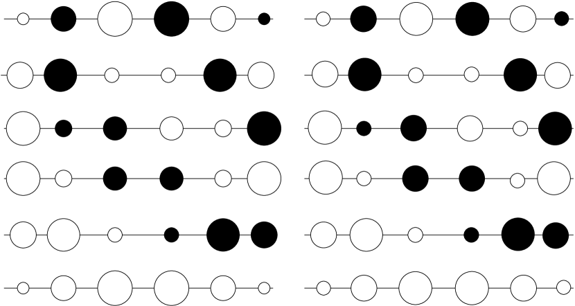
Figure 5: Natural orbitals of the 6-site Hubbard chain for U=0 (left) and U/t=8 (right). The radius of each sphere is proportional to the amplitude of the natural orbital, and the area is proportional to the site occupation. Full and open circles represent the different signs of the orbital coefficients. The orbitals are arranged with decreasing occupation from bottom to top. For each spatial orbital shown, there are two spin orbitals.

However, the interaction strength has a strong effect on the occupations as shown in figure 6. While the occupations in the (non-degenerate) ground state of a non-interacting system are always either zero or one, all occupations become fractional if the interaction is switched on. From a chemical point of view, the depopulation of bonding orbitals and the population of formerly unoccupied antibonding orbitals reflects the depression of the covalent interaction by the interaction. From a solid-state point of view, the behavior seen in Fig. 6 is reminiscent of the momentum distribution functions of a Fermi-liquid or the Luttinger liquid. While for noninteracting particles the momentum distribution has a sharp drop of the occupations from one to zero at the Fermi momentum, for the interacting electron systemm, it exhibits a gradual decrease with either a drop of size $Z^{-1}<1$, the quasi-particle renormalization factor of a Fermi liquid, or, for a Luttinger liquid, a sharp change with an algebraic singularity at the Fermi momentum

Figure 6: Occupations $f_{n}$ of the natural orbitals as function of the interaction strength from our theory (circles) compared to exact result. The occupations become more equally distributed with increasing interaction strength.

The smearing out of the occupations implies that the number of one-particle wave functions to be considered must be larger than that required for density-functional theory. If we venture into an extrapolation of our findings to real systems, we expect that it will be necessary to include one-particle wave functions $|\psi_{n}\rangle$ up to the antibonding orbitals of bonds for which left-right correlation is important. This implies that we need to include orbitals up to several electron volts above the Fermi-level. Working in our favor is that in the strongest bonds, with high-lying antibonding states, the kinetic energy is large and therefore dominating over the Coulomb repulsion. Correlations are dominant in relatively weak bonds, either when they are stretched to the dissociation limit, or when they involve d- and f-electron orbitals or $\pi$ bonds.

One of the major problems plaguing density-functional calculations is the band-gap problem. Here, we do not refer to the optical band gap, which is an excited state property and which, in a strict sense, is neither accessible by ground-state DFT nor by our theory. Instead we investigate here the thermodynamic gap, which we define as

$$\Delta=\lim_{\delta\rightarrow 0}\biggl{(}\left.\frac{dE}{dN}\right|_{N+\delta}-\left.\frac{dE}{dN}\right|_{N-\delta}\biggr{)}\,.$$

Because $E(N)$ is a series of line-segments interpolating between the values for integer particle numbers $N$, this definition is identical to the more common expression $\Delta=E(N+1)-2E(N)+E(N-1)$, which is the difference $\Delta=A-I$ between electron affinity $A$ and ionization potential $I$. Because $E(N)$ is a true ground-state property, it should be properly described both by our theory and by correct density-functional theory. A failure of describing the thermodynamic gap has a fundamental impact on the defect chemistry in semiconductors and insulators.

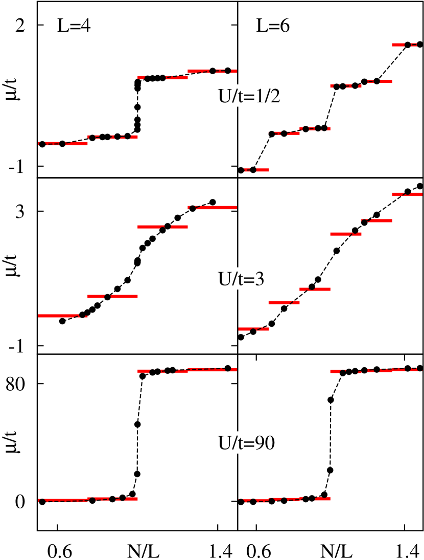
Figure 7: Chemical potentials $\mu$ versus filling $N/L$ from our theory (spheres and dashed lines) and the exact Hubbard chain (solid lines) for the four-site (left) and the six-site (right) Hubbard chains as function of the particle number for $U/t=1/2$, $U/t=3$ and $U/t=90$ from top to bottom. The dashed lines are a guide to the eye and connect the data points. (Color online)

The chemical potential $\mu(N)=\frac{dE}{dN}$ for different interaction strengths calculated with our theory is shown in figure 7 and compared to the exact thermodynamic band gap, included as horizontal lines in the figure. It is obvious that our theory does not yield a discontinuity. Despite of this, the value of the band band gap can nevertheless be obtained using Slater’s transition rule as $\Delta=\mu(N+\frac{1}{2})-\mu(N-\frac{1}{2})$ from the difference of the chemical potentials at half-integer occupations.

Figure 8: Total energy for fractional particle numbers N divided by the number of sites L of the Hubbard chains for $U/t=1/2$ (first panel), $U/t=3$ (second) and $U/t=90$ (third). Symbols denote results from our theory, lines the exact behavior.

The failure to describe the discontinuity of the chemical potential, and thus the band gap, reminds of the behavior of approximate density-matrix functionals.Helbig et al. (2007) These functionals do not make the local approximation, but use approximate numerical representations of the exchange correlation energy. Also here, the discontinuity vanishes, while the band gap calculated with half-occupied orbitals are satisfactory predictions.

Except for the non-interacting case, the total energy appears to be a continuous function of the particle number within our theory, while the exact result has jumps in the slope at integer fillings. We attribute this deficiency of our theory to its tendency to underestimate the total energy. As seen in figure 8 this underestimation is most prominent for fractional particle numbers at intermediate interaction strengths. For small or huge values of $U$ the effect is less visible; but here, too, the variation across integer fillings is smooth, as it is apparent from Fig. 7. As discussed in appendix A this defect is related to the fact that the wave function for each Anderson-impurity model is optimized individually. An approximation based on a common wave function for all sites may direct towards a remedy of this problem.

V Conclusion

We proposed a pathway to include explicit correlations into density-functional based calculations. The guiding ideas have been to develop a strict variational approximation of the interacting electron gas, that avoids the dimensional bottleneck of may-particle quantum theory, and that allows seamless incorporation into electronic structure methodology of density-functional theory.

Let us summarize what we have accomplished so far: Based on a general formulation using a density-matrix-functional description of the solid, the many-particle problem for the lattice with the full interaction has been replaced by a collection of generalized multi-orbital Anderson impurity models, defined through the functionals $F^{W_{R}}$, see Eq. (26). These Anderson impurity models are defined relative to the DFT functional as accurate way to obtain the quasi-particle dispersion including effects of non-local correlations and proper screening. Since the local DFT contributions can be explicitly subtracted from the density-matrix functional, the problem of double counting can be treated without further assumptions in this approach. Restricting the actual correlations to one site only has proven to be a powerful idea in many-particle schemes such as Dynamical Mean-Field theory. We believe that the density-matrix functional approach plus local approximation as proposed in this paper, when properly implemented, will provide a tool to treat correlation effects in a spirit similar to DMFT, however using the information of the density-matrix only.

As test case we applied our method to finite Hubbard chains as simple model systems. The extremalization of the the density-matrix functional is done on the fly using an explicit constrained-search algorithmLevy (1979). This iterative approach has been solved by a dynamical approach inspired by the Car-Parrinello method. The iterative nature of the constrained-search algorithm holds promise to important cost reductions in an outer self-consistency loop.

In contrast to static mean-field theory, our method produces at half filling the correct singlet state with strong anti-ferromagnetic correlations, and thus gives a qualitative description of left-right correlation. The local approximation smears out the band-gap, which has been observed similarly in approximate density-matrix functionals. The energy levels of the many-particle system are, however, well approximated using the chemical potentials half-integer particle numbers.

Presently, each of these Anderson impurity models still represents a nontrivial many-particle problem on the infinite lattice. Thus, apparently nothing has been gained so far regarding a calculation of physical properties in this approximation. The important next step now is to reformulate the effective quantum impurity problem in a way that it can be solved efficiently. In standard DMFT the important aspect is that the actual lattice structure only enters through the density of states. As consequence, the solution of the effective quantum impurity problem can be done without ever resorting to the actual lattice.

It is obviously important to develop a similar approach for the local density-matrix functional. The most straightforward idea here would be to treat the quantum impurity as open quantum system and apply techniques developed in this field to facilitate the creation of an efficient impurity solver for our theory.

Appendix A Local approximation

Here we show that distributing the interaction into many Anderson-impurity models leads to an underestimation of the energy, i.e.

$$F^{\sum_{R}\hat{W}_{R}}[{\bm{\rho}}]\geq\sum_{R}F^{\hat{W}_{R}}[{\bm{\rho}}]\,.$$ (45)

Let $|\Phi_{0}[{\bm{\rho}}]\rangle$ be the ground-state wave function for the interaction $\sum_{R}\hat{W}_{R}$ and a one-particle term $\hat{h}_{0}$ so that

$$\left[\hat{h}_{0}[{\bm{\rho}}]+\sum_{R}\hat{W}_{R}-\mathcal{E}_{0}[{\bm{\rho}}]\right]|\Phi_{0}[{\bm{\rho}}]\rangle=0\,.$$ (46)

The one-particle term $\hat{h}_{0}[{\bm{\rho}}]$ is determined such that $|\Phi_{0}[{\bm{\rho}}]\rangle$ produces the specified reduced density matrix $\bm{\rho}$. Let furthermore $|\Phi_{R}[{\bm{\rho}}]\rangle$ be the ground-state wave function with only a local interaction on site $R$ and with the specified reduced density matrix:

$$\left[\hat{h}_{R}[{\bm{\rho}}]+\hat{W}_{R}-\mathcal{E}_{R}[{\bm{\rho}}]\right]|\Phi_{R}[{\bm{\rho}}]\rangle=0\,.$$ (47)

With these definitions, we obtain the desired inequality Eq. 45:

$$F^{\sum_{R}\hat{W}_{R}}[{\bm{\rho}}]=\sum_{R}\biggl{\langle}\Phi_{0}[{\bm{\rho}}]\biggr{|}\hat{W}_{R}\biggl{|}\Phi_{0}[{\bm{\rho}}]\biggr{\rangle}$$

$$\geq\sum_{R}\biggl{\langle}\Phi_{R}[{\bm{\rho}}]\biggr{|}\hat{W}_{R}\biggl{|}\Phi_{R}[{\bm{\rho}}]\biggr{\rangle}=\sum_{R}F^{\hat{W}_{R}}[{\bm{\rho}}]\,.$$ (48)

The argument rests on the simple fact that the energy decreases, if one optimizes wave functions for each impurity model individually, rather than to select one wave function that needs to suit all local interactions simultaneously.

References

- Hohenberg and Kohn (1964) P. Hohenberg and W. Kohn, Phys. Rev. 136, 864 (1964).
- Kohn and Sham (1965) W. Kohn and L. Sham, Phys. Rev. 140, 1133 (1965).
- Stewart (1984) G. R. Stewart, Rev. Mod. Phys. 56, 755 (1984).
- Imada et al. (1998) M. Imada, A. Fujimori, and Y. Tokura, Rev. Mod. Phys. 70, 1039 (1998).
- Dagotto (1994) E. Dagotto, Rev. Mod. Phys. 66, 763 (1994).
- Salamon and Jaime (2001) M. B. Salamon and M. Jaime, Rev. Mod. Phys. 73, 583 (2001).
- v. Löhneysen et al. (2007) H. v. Löhneysen, A. Rosch, M. Vojta, and P. Wölfle, Rev. Mod. Phys. 79, 1015 (2007).
- Hubbard (1963) J. Hubbard, Proc. Roy. Soc. London A 276, 238 (1963).
- Kanamori (1963) J. Kanamori, Prog. Theor. Phys. 30, 275 (1963).
- Gutzwiller (1963) M. C. Gutzwiller, Phys. Rev. Lett. 10, 159 (1963).
- Aryasetiawan and Gunnarsson (1998) F. Aryasetiawan and O. Gunnarsson, Rep. Prog. Phys. 61, 237 (1998).
- Anisimov et al. (1991) V. Anisimov, J. Zaanen, and O. Andersen, Phys. Rev. B 44, 943 (1991).
- Becke (1993) A. D. Becke, J. Chem. Phys. 98, 1372 (1993).
- Rollmann et al. (2004) G. Rollmann, A. Rohrbach, P.Entel, and J. Hafner, Phys. Rev. B 69, 165107 (2004).
- Georges et al. (1996) A. Georges, G. Kotliar, W. Krauth, and M. J. Rozenberg, Rev. Mod. Phys. 68, 13 (1996).
- Pruschke et al. (1995) T. Pruschke, M. Jarrell, and J. K. Freericks, Adv. in Phys. 44, 187 (1995).
- Obermeier et al. (1997) T. Obermeier, T. Pruschke, and J. Keller, Phys. Rev. B 56, R8479 (1997).
- Zitzler et al. (2002) R. Zitzler, T. Pruschke, and R. Bulla, Eur. Phys. J. B 27, 473 (2002).
- Pruschke (2005) T. Pruschke, Prog. Theo. Phys. Suppl. 160, 274 (2005).
- Maier et al. (2005) T. A. Maier, M. Jarrell, T. Pruschke, and M. Hettler, Rev. Mod. Phys. 77, 1027 (2005).
- Kotliar and Vollhardt (2004) G. Kotliar and D. Vollhardt, Physics Today 57, 53 (2004).
- Kotliar et al. (2006) G. Kotliar, S. Y. Savrasov, K. Haule, V. S. Oudovenko, O. Parcollet, and C. A. Marianetti, Rev. Mod. Phys. 78, 865 (2006).
- Held et al. (2006) K. Held, I. A. Nekrasov, G. Keller, V. Eyert, N. Blümer, A. K. Mcmahan, R. T. Scalettar, T. Pruschke, V. I. Anisimov, and D. Vollhardt, phys. stat. sol. (b) 243, 2599 (2006).
- Savrasov et al. (2001) S. Y. Savrasov, G. Kotliar, and E. Abrahams, Nature 410, 793 (2001).
- Anisimov et al. (2005) V. Anisimov, D. Kondakov, A. Kozhevnikov, I. Nekrasov, Z. Pchelkina, J. Allen, S. Mo, H. Kim, P. Metcalf, S. Suga, et al., Phys Rev B 71, 125119 (2005).
- Lechermann et al. (2006) F. Lechermann, A. Georges, A. Poteryaev, S. Biermann, M. Posternak, A. Yamasaki, and O. K. Andersen, Phys Rev B 74, 125120 (2006).
- Jacob et al. (2008) D. Jacob, K. Haule, and G. Kotliar, Epl-Europhys Lett 84, 57009 (2008).
- Amadon et al. (2008) B. Amadon, F. Lechermann, A. Georges, F. Jollet, T. O. Wehling, and A. I. Lichtenstein, Phys Rev B 77, 205112 (2008).
- Haule et al. (2010) K. Haule, C.-H. Yee, and K. Kim, Phys. Rev. B 81, 195107 (2010).
- Aryasetiawan et al. (2004) F. Aryasetiawan, M. Imada, A. Georges, G. Kotliar, S. Biermann, and A. Lichtenstein, Phys Rev B 70, 195104 (2004).
- Gilbert (1975) T. Gilbert, Phys. Rev. B 12, 2111 (1975).
- Müller (1984) A. Müller, Phys. Lett. 105A, 446 (1984).
- Goedecker and Umrigar (1998) S. Goedecker and C. Umrigar, Phys. Rev. Lett 81, 866 (1998).
- Csanyi and Arias (2000) G. Csanyi and T. Arias, Phys. Rev. B 61, 7348 (2000).
- Buijse and Baerends (2002) M. Buijse and E. Baerends, Mol. Phys. 100, 401 (2002).
- Gritsenko et al. (2005) O. Gritsenko, K. Pernal, and E. Baerends, J. Chem. Phys. 122, 204102 (2005).
- Sharma et al. (2008) S. Sharma, J. Dewhurst, N. Lathiotakis, and E. K. U. Gross, Phys. Rev. B 78, 201103 (2008).
- Car and Parrinello (1985) R. Car and M. Parrinello, Phys. Rev. Lett 55, 2471 (1985).
- Blöchl (1994) P. Blöchl, Phys. Rev. B 50, 17953 (1994).
- Coleman (1963) A. Coleman, Rev. Mod. Phys. 35, 668 (1963).
- Löwdin (1955) P.-O. Löwdin, Phys. Rev. 97, 1474 (1955).
- Levy (1979) M. Levy, Proc. Nat’l Acad. Sci. USA (1979).
- Anderson (1961) P. W. Anderson, Phys. Rev. 124, 41 (1961).
- Harris and Jones (1974) J. Harris and R. Jones, J. Phys. F: Met. Phys. 4, 1170 (1974).
- Bahmann and Ernzerhof (2008) H. Bahmann and M. Ernzerhof, J. Chem. Phys. 128, 234104 (2008).
- Perdew et al. (1996) J. Perdew, K.Burke, and Y. Wang, Phys. Rev. B 54, 16533 (1996).
- Dederichs et al. (1984) P. H. Dederichs, S. Blügel, R. Zeller, and H. Akai, Phys. Rev. Lett 53, 2512 (1984).
- Verlet (1967) L. Verlet, Phys. Rev. 159, 98 (1967).
- Ryckaert et al. (1977) J.-P. Ryckaert, G. Cicotti, and H. J. C. Berendsen, J. Comp. Phys. 23, 327 (1977).
- Kolos and Roothaan (1960) W. Kolos and C. Roothaan, Rev. Mod. Phys. 32, 205 (1960).
- Helbig et al. (2007) N. Helbig, N. Lathiotakis, M. Albrecht, and E. Gross, Europhys. Lett. 77, 67003 (2007).