Zigzag graphene nanoribbon edge reconstruction with Stone-Wales defects

Abstract

In this article, we study zigzag graphene nanoribbons with edges reconstructed with Stone-Wales defects, by means of an empirical (first-neighbor) tight-binding method, with parameters determined by ab-initio calculations of very narrow ribbons. We explore the characteristics of the electronic band structure with a focus on the nature of edge states. Edge reconstruction allows the appearance of a new type of egde states. They are dispersive, with non-zero amplitudes in both sub-lattices; furthermore, the amplitudes have two components that decrease with different decay lengths with the distance from the edge; at the Dirac points one of these lengths diverges, whereas the other remains finite, of the order of the lattice parameter. We trace this curious effect to the doubling of the unit cell along the edge, brought about by the edge reconstruction. In the presence of a magnetic field, the zero-energy Landau level is no longer degenerate with edge states as in the case of pristine zigzag ribbon.

I Introduction

At the present time, the most promising scalable growth methods of graphene films are either based on epitaxial growth on silicon carbide Berger et al. (2004); First et al. (2010) or on chemical vapor deposition (CVD) of graphene on metal surfaces.Li et al. (2009); Reina et al. (2009); Kim et al. (2009); Bae et al. (2010) Yet, the latter methods do not produce graphene films with electronic mobilities as high as those reported for exfoliated graphene. Novoselov et al. (2004, 2005) Electronic transport Castro Neto et al. (2009); Peres (2010) in CVD-grown graphene is hindered by grains, grain boundaries and atomic patchwork quilts,Huang et al. (2011); Nemes-Incze et al. (2011) which can be interpreted as topological defects.Vozmediano et al. (2010); Banhart et al. (2011)

CVD-grown materials are in general polycrystalline in nature, having their physical properties dominated by the grain boundaries’ size. The situation is no different for graphene. For this material, it is theoretically expected that some of its electronic properties will be markedly different from its exfoliated counterpart, as suggested by calculations of formation energies of different types of grain boundariesLiu and Yakobson (2010) and by the transport measurements and theoretical calculationsFerreira et al. (2010) in high-quality CVD-grownBae et al. (2010) graphene.

Due to graphene’s hexagonal structure, originated from the sp² bonds, the grain boundaries are expected to be formed of pentagons-heptagons pairs, known as Stone-Wales (SW) defects.Stone and Wales (1986) Recent atomic resolution TEM studiesMeyer et al. (2008); Lahiri et al. (2010); Huang et al. (2011) have allowed to visualize grain boundaries in CVD-grown graphene. These experimental studies have shown that the grain boundaries are not perfectly straight lines and that the 5-7 defects along the boundaries are not periodic. These type of defects have a profound effect on the threshold for mechanical failure of the graphene membranes, which is reduced by an order of magnitude, relatively to the exfoliated membranes. In what concerns the electronic properties, it has been shown that the measured electronic mobilities depend on the details of the CVD-growth recipes. Li et al. (2009); Reina et al. (2009); Bae et al. (2010); Huang et al. (2011)

Furthermore, as shown by recent TEM studies,Huang et al. (2011) these extended pentagons-heptagons pairs defect lines intercept each other at random angles, forming irregular polygons with edges showing stochastic distribution of length, making it extremely difficult to make theoretical studies of these defects using microscopic tight-binding models. On a different tone, it has been argued that these defect lines can act as one-dimensional conducting charged wires.Lahiri et al. (2010); Bahamon et al. (2011) The charging of these topological wires is achieved by the self-doping mechanism. Peres et al. (2006)

As said, studying Stone-Wales defects in the bulk of graphene, using microscopic tight-binding models, is a difficult task, due to the breaking of translational geometry. On the other hand, the grain boundary formed by the 5-7 defect lines effectively create an edge, giving rise to an enhanced density of statesLahiri et al. (2010); Bahamon et al. (2011) at the Dirac point, all in all equal to what is found at the edges of zigzag nanoribbons. Nakada et al. (1996); Fujita et al. (1996); Wakabayashi et al. (1999, 2010) Evading the difficulty of studying topological defects in the bulk of graphene, we take, in this article, the approach of studying the formation of Stone-Wales defects at the edges of zigzag nanoribbons, supported by the experimental findings that grain boundaries effectively act as edges of the crystalline grain.Lahiri et al. (2010); Bahamon et al. (2011) We will be focusing our study on the electronic properties of graphene nanoribbons close to the Dirac point, for the effect of Stone-Wales defects have their largest impact on the properties of graphene at low energies.

Ab-initio calculations have shown that when SW defects are present in graphene nanoribbons (GNRs), the energy decreases as the defect gets closer to the edge of the ribbon.Huang et al. (2009) Other first principles studies have shown that the formation of SW defects at the edges of both armchair and zigzag GNRs (respectively, AGNRs and ZGNRs), stabilize them both energetically and mechanically.Huang et al. (2009); Koskinen et al. (2008); Bhowmick and Waghmare (2010) The zigzag edge, in particular, is metastable under total reconstruction with SW defects, and a planar reconstruction spontaneously takes place at room temperature.Koskinen et al. (2008); Lee et al. (2010)

Edge-reconstructed ZGNRs by means of SW defects, are claimed to be stable only at very low hydrogen pressure (well below the hydrogen pressure at ambient conditions) and very low temperatures.Wassmann et al. (2008) However, reconstructions of the zigzag (as well as armchair) edges have been recently observed with high-resolution TEM.Koskinen et al. (2009); Ç. Girit et al. (2009); Chuvilin et al. (2009) The recent work of Suenaga et al.,Suenaga and Koshino (2010) on single-atom spectroscopy using low-voltage STEM, may be used as yet another mean of identifying edge reconstructions of graphene ribbons. Moreover, refinements in other techniques, such as Raman spectra of the edges,Malola et al. (2009) STM images of the edges,Koskinen et al. (2008) and coherent electron focusing,Rakyta et al. (2010) may help in the identification of these kinds of edge reconstructions.

In this work, we have studied various reconstructions of zigzag edges with SW defects, namely $zz(57)$, $zz(576)$ and $zz(5766)$ (see Fig. 1). However, in this article, we give special emphasis to the case of total reconstruction of the zigzag edges, $zz(57)$, because it is the most stable configuration in the absence of hydrogen passivation.Wassmann et al. (2008); Koskinen et al. (2008); Huang et al. (2009)

Figure 1: SW-reconstructed zigzag edges: the pristine zigzag edge in $(a)$, also known as $zz$ edge; the $zz(57)$ edge in $(b)$; the $zz(576)$ in $(c)$; the $zz(5766)$ in $(d)$;

This article is organized as follows: In section II, we study the electronic structure of wide zigzag ribbons, with edges reconstructed by Stone-Wales defects, using an empirical tight-binding model. In Subsection II.1, we start by computing the model parameters using the results of ab-initio simulations. Based on the empirical tight-binding model presented in Subsection II.2, we study the electronic structure of ZGNRs whose edges were reconstructed by SW defects, with a focus on the edge states showing up in these systems (Subsection II.3). We find that some modifications (relatively to the pristine ZGNR) are introduced in the electronic structure, as well as, that the edge states of the edge reconstructed ZGNRs are distinct from those of the pristine ZGNRs. Finally, in Subsection II.4, we explore the implications of the presence of a magnetic field directed perpendicularly to the ribbon plane, in the electronic structure and edge states of a zigzag ribbon, pinpointing the modifications originating from the edge reconstruction.

II Tight-binding study of ribbons with reconstructed edges

In this Section, the main issue under discussion is the behavior of the edge states of wide zigzag ribbons, whose edges have been reconstructed due to the formation of edge Stone-Wales defects (see Fig. 1). The huge amount of computational resources needed to study large physical systems employing ab-initio methods, makes it prohibitive to explore the physics of wide ribbons using such techniques. An alternative approach, is to use phenomenological tight-binding models, which being computationally not so demanding also give a microscopic understanding of the electronic properties of these types of systems.

In order to provide an accurate (tight-binding) description of the reconstructed edges, we start by performing ab-initio simulations of narrow ribbons, from which we extract the values of the hopping amplitudes at the edge. These hopping amplitudes are posteriorly used in the construction of the tight-binding Hamiltonian, in which the study of the edge states for large ribbons is based on.

II.1 Parametrization of the hopping amplitudes using ab-initio methods

We used Density Functional Theory (DFT) to parametrize the tight-binding. The calculations were performed using the code aimpro,Rayson and Briddon (2008) under the Local Density Approximation. The Brillouin-zone (BZ) was sampled for integrations according to the scheme proposed by Monkhorst-Pack.Monkhorst and Pack (1976) The core states were accounted for by using the dual-space separable pseudo-potentials by Hartwigsen, Goedecker, and Hutter.Hartwigsen et al. (1998) The valence states were expanded over a set of $s$-, $p$-, and $d$-like Cartesian-Gaussian Bloch atom-centered functions. The k-point sampling was $16\times 2\times 1$ and the atoms were relaxed in order to find the equilibrium positions. A supercell with orthorhombic symmetry was used; the cell parameter in the infinite direction was $4.885\mathring{A}$. A vacuum layer of $12.7\mathring{A}$ in the nanoribbon plane and $10.6\mathring{A}$ in the normal direction were used in order to avoid interactions between nanoribbons in different unit cells.

In what follows, we will focus on the ZGNR with totally reconstructed edges, the most stable of this family of reconstructions in the absence of hydrogen passivation (see Fig. 1).Wassmann et al. (2008); Koskinen et al. (2008); Huang et al. (2009) Note that the dangling bonds that are on the origin of the zigzag edge reactiveness, are eliminated by the reconstruction of the edge, forming triple bonds between the outer carbon atoms at the edges ($h_{2}$ bond in Fig. 4). In the literature, the SW totally reconstructed edge is usually named as $zz(57)$. Note that the unit cell of such a ZGNR has twice the size of the unit cell of the pristine ZGNR (see Fig. 3). The generalization of the following study for SW edge reconstructions, other than $zz(57)$, for example $zz(576)$, $zz(5766)$, etc., is straightforward.

In Fig. 2, we show the relaxed edge geometry of a totally reconstructed edge (in absence of hydrogen passivation), $zz(57)$, as obtained from the ab-initio calculations, together with the inter-carbon distances and the angles between carbon bonds.

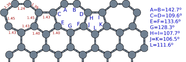
Figure 2: Relaxed edge geometry of the totally reconstructed zigzag edge (in absence of hydrogen passivation), $zz(57)$, obtained from the ab-initio calculations. The numbers refer to the bond lengths in angstroms; the capital letters refer to the angles between two adjacent bonds.

The procedure for determining the hopping amplitudes at the reconstructed edge is the following. From ab-initio calculations one obtains the different carbon-carbon distances at the edges of the ribbons as well as the values of the angles between carbon bonds (see Fig. 2). In the case of the $zz(57)$ edge reconstruction, our first principles calculations show that the ribbons remain planar (we have allowed the system to relax along the three spatial dimensions); therefore the values of the angles in Fig. 2 play no role in the determination of the hopping amplitudes, since these arise from $pp\pi$ hybridization. Using the carbon-carbon distances, we compute the hopping amplitudes using the parametrizationTang et al. (1996)

$$\tau(r_{ij})=\big{(}\frac{r_{ij}}{a_{0}}\big{)}^{-\alpha_{2}}\exp[-\alpha_{3}\times(r_{ij}^{\alpha_{4}}-a_{0}^{\alpha_{4}})],$$ (1)

where $r_{ij}$ stands for the distance between the carbons labeled by $i$ and $j$ (given in unities of Angströms), the adimensional parameters $\alpha_{2}=1.2785$, $\alpha_{3}=0.1383$, $\alpha_{4}=3.4490$, while $a_{0}$ is the carbon-carbon distance in the bulk (in units of Angströms).Tang et al. (1996) The hopping renormalizations, $h_{i}$, $h_{i}^{\prime}$ and $v_{i}$, (see Fig. 4 for their definition) are given by the $\tau(r_{ij})$ for the corresponding carbon-carbon distances at the edge. For the $zz(57)$ edge, in the absence of passivation, the values of these renormalizations are listed in Table 1.

$h_{1}$	$h_{2}$	$h_{3}$	$h_{4}$	$h_{1}^{\prime}$	$h_{2}^{\prime}$	$h_{3}^{\prime}$	$h_{4}^{\prime}$	$v_{1}$	$v_{2}$
1.06	1.42	1.06	0.94	0.98	0.98	1.04	1.04	0.94	0.94

Table 1: Values of the hoppings in unities of $t$ (which we also call hopping renormalizations) for a $zz(57)$ (see Fig. 2 and Fig. 4) calculated from the C-C distances obtained from the DFT numerical calculations using Eq. (1).

II.2 The Tight-Binding Hamiltonian of a ZGNR with $zz(57)$ edges

The simplest model one can construct describing non-interacting electrons in a ZGNR whose edges have been reconstructed by SW defects is the first neighbor tight-binding (TB) model. Generically, a ribbon has $N$ zigzag rows of atoms along the longitudinal direction ($0\leq n\leq N-1$) and, in each unit cell, there are $P$ zigzag columns of atoms ($1\leq p\leq P$). In the case of a $zz(57)$ edge, $P=2$.

The TB Hamiltonian for the edge reconstructed ZGNR, can be written as

$$H = H^{U}+H^{bulk}+H^{L},$$ (2)

where $H^{U}$ stands for the Hamiltonian of the region in the vicinity of the upper edge of the ribbon (at $n=0$ in Fig. 3), $H^{L}$ stands for the region in the vicinity of the lower edge (at $n=N-1$ in Fig. 3) and $H^{bulk}$ stands for the bulk of the ribbon.

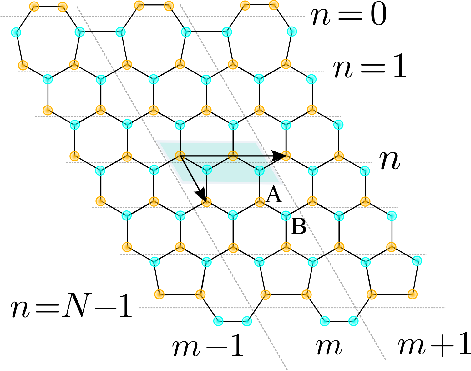
Figure 3: Scheme of a ZGNR with its edges totally reconstructed by SW defects [a $zz$(57) ribbon]. Details of the edge are represented in Fig. 4.

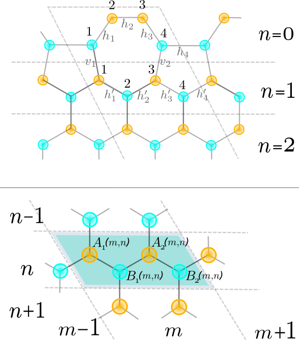
Figure 4: Details of the ZGNR with its edges totally reconstructed by SW defects, $zz(57)$. The $h_{i}$, $h_{i}^{\prime}$ and $v_{i}$ stand for the factors giving the renormalization of the hoppings, $t$, between nearest neighbors in the vicinity of the defect. We omit the lower edge because it is analogous to the upper one.

The ab-initio results (see Fig. 2) show that only in the first two rows are the hopping parameters between two adjacent carbon atoms different from their usual value in the bulk. Thus, we choose to identify term $H^{U}$ ($H^{L}$) in the full Hamiltonian with the two upper (lower) rows of atoms of the ribbon. The annihilation operators of the four numbered atoms in row $n=0$ (see Fig. 4), are denoted by $d_{1}(m)$, $d_{2}(m)$, $d_{3}(m)$, and $d_{4}(m)$, while those referring to the four numbered atoms in row $n=1$, are denoted by $c_{1}(m)$, $c_{2}(m)$, $c_{3}(m)$, and $c_{4}(m)$.

For the sake of clarity, we will separate in $H^{U}$ the terms referring to each row, $n=0$ and $n=1$, and to the coupling between them, $H^{U}=H_{n=0}^{U}+H_{n=1}^{U}+H_{c}^{U}$. For row $n=0$, we have

$$H_{n=0}^{U} = -t\sum_{m}\bigg{\{}\sum_{i=1}^{3}\Big{[}h_{i}d_{i}^{\dagger}(m)d_{i+1}(m)\Big{]}$$ (3)

$$+ h_{4}d_{4}^{\dagger}(m)d_{1}(m+1)+{\rm h.c.}\bigg{\}},$$

while for row $n=1$,

$$H_{n=1}^{U} = -t\sum_{m}\bigg{\{}\sum_{i=1}^{3}\Big{[}h_{i}^{\prime}c_{i}^{\dagger}(m)c_{i+1}(m)\Big{]}$$ (4)

$$+ h_{4}^{\prime}c_{4}^{\dagger}(m)c_{1}(m+1)\Big{]}+{\rm h.c.}\bigg{\}},$$

and for the coupling between row $n=0$ and row $n=1$,

$$H_{c}^{U} = -t\sum_{m}\Big{[}v_{1}c_{1}^{\dagger}(m)d_{1}(m)+v_{2}c_{3}^{\dagger}(m)d_{4}(m)\Big{]}+{\rm h.c.}.$$

Recall from Table 1 that $h_{1}=h_{3}$, $h_{1}^{\prime}=h_{2}^{\prime}$, $h_{3}^{\prime}=h_{4}^{\prime}$, and $v_{1}=v_{2}$.

The term $H^{bulk}$, corresponding to the Hamiltonian of the bulk (between row $n=2$ and $n=N-3$), is given by

$$H^{bulk} = -t\sum_{m}\sum_{n=2}^{N-3}\bigg{(}\Big{[}a_{1}^{\dagger}(m;n)+a_{2}^{\dagger}(m;n)$$

$$+ a_{1}^{\dagger}(m;n+1)\Big{]}b_{1}(m;n)+\Big{[}a_{2}^{\dagger}(m;n)$$

$$+ a_{1}^{\dagger}(m+1;n)+a_{2}^{\dagger}(m;n+1)\Big{]}b_{2}(m;n)+{\rm h.c.}\bigg{)},$$

where $a_{p}(m;n)$ [$b_{p}(m;n)$] is the annihilation operator of an electron state localized at the atom of sub-lattice $A$ ($B$) in column $p$ ($p=1,\,2$ for a $zz(57)$ edge) and row $n$, of the unit cell labeled by $m$. The term $H^{L}$ describing the lower edge is analogous to the upper edge term, $H^{U}$. Recall that the $h_{i}$, $v$ and $h_{i}^{\prime}$ parameters in the equations defining the tight-binding Hamiltonian correspond to the values of the hoppings in units of $t$. In addition, we make the following identifications:

$$d_{1(4)}(m) \to b_{1(2)}(m;0),$$

$$d_{2(3)}(m) \to a_{1(2)}(m;0),$$

$$c_{1(3)}(m) \to a_{1(2)}(m;1),$$

$$c_{2(4)}(m) \to b_{1(2)}(m;1).$$

With no loss of generality, we assume periodic boundary conditions along the ribbon $x$-direction. This simplification allows us to diagonalize the Hamiltonian with respect to $m$ by Fourier transforming $H$ along the $x$-direction,

$$H=\sum_{k}H_{k}=\sum_{k}\big{[}H_{k}^{U}+H_{k}^{bulk}+H_{k}^{L}\big{]}\,.$$ (7)

Having determined the values of the $h_{i}$, $v$ and $h^{\prime}_{i}$ (see Table 1), we compare in Fig. 5 the obtained low-energy spectrum from the ab-initio calculations with that resulting from the numerical diagonalization of the tight-binding Hamiltonian $H_{k}$, Eq. (7).

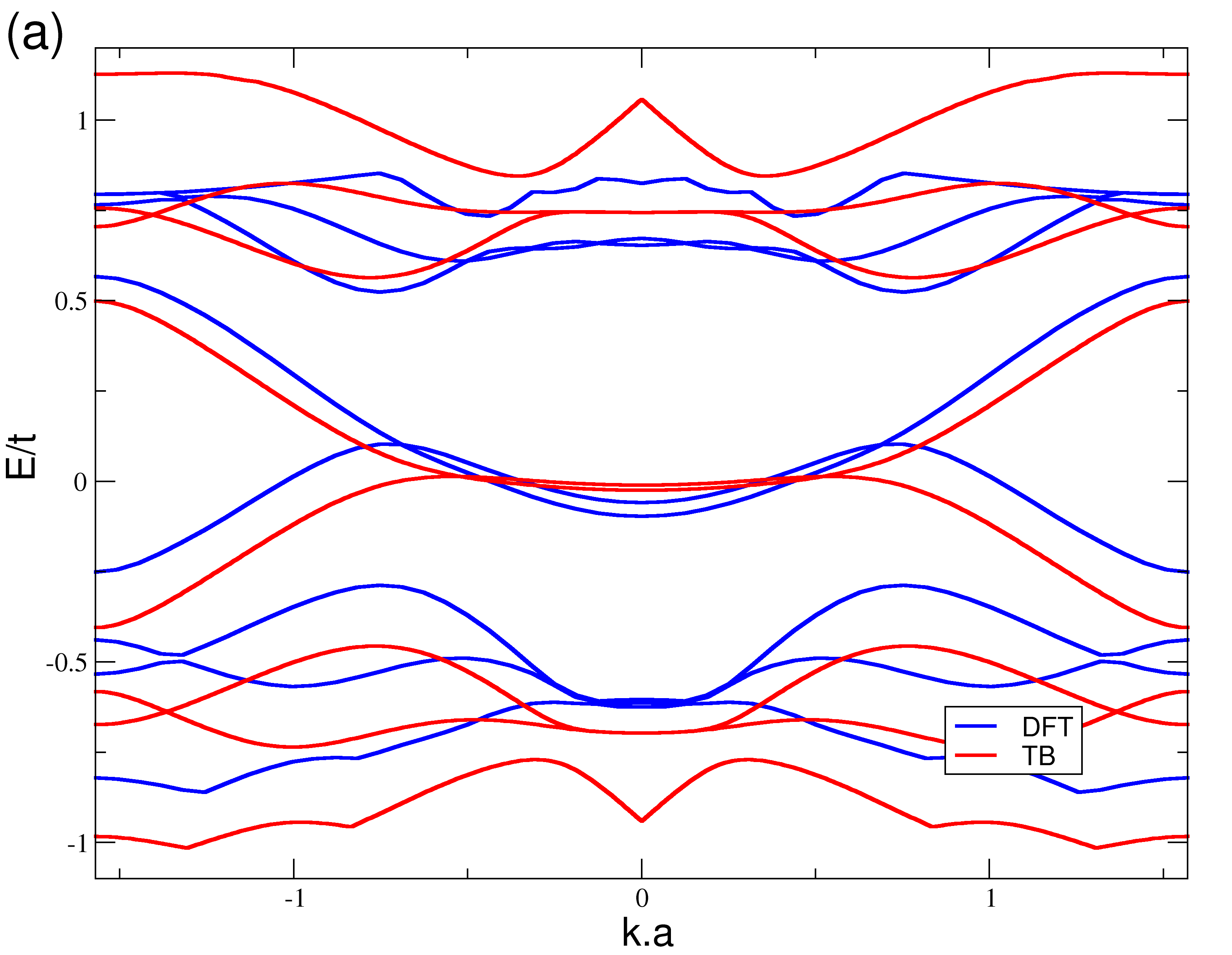
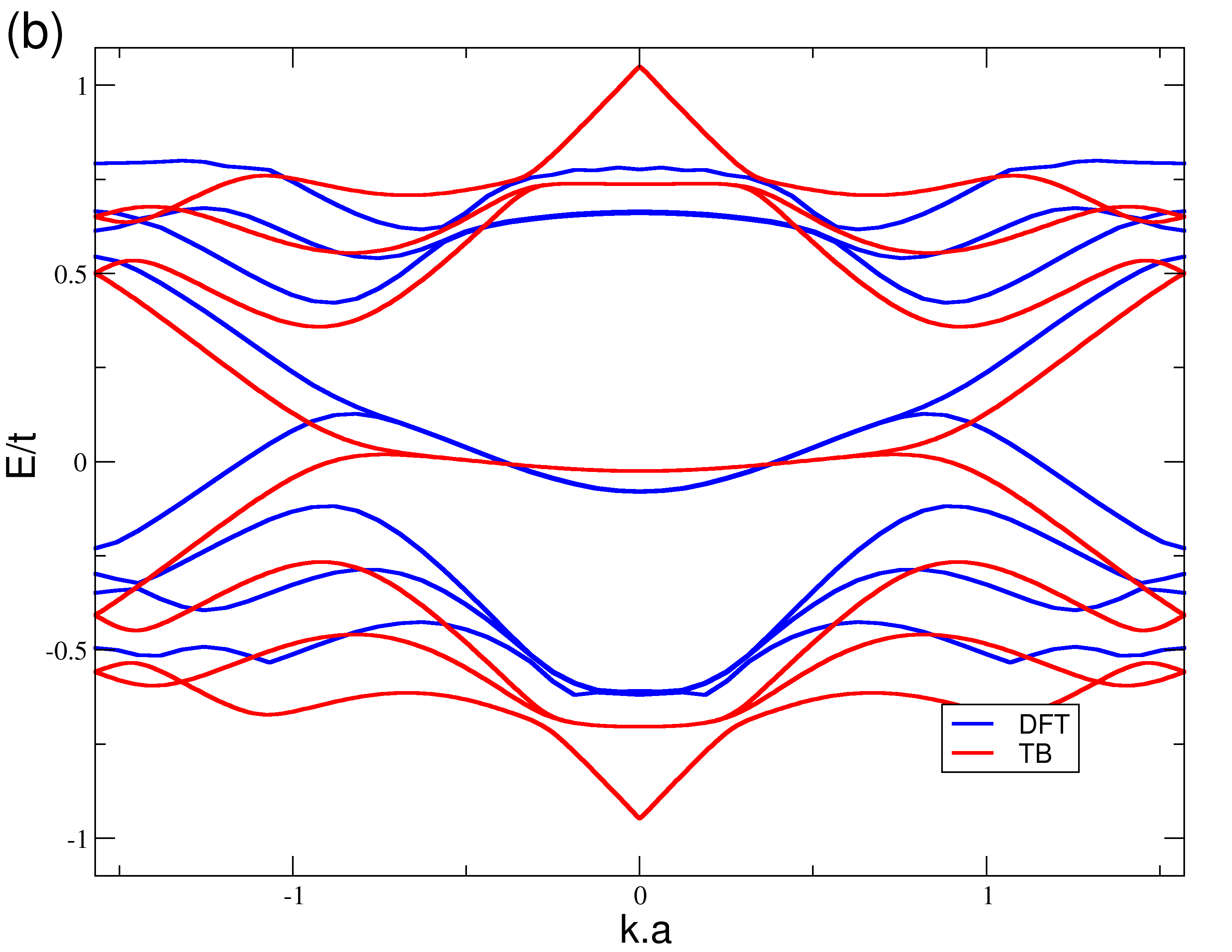
Figure 5: Comparison between the low-energy spectrum of a ZGNR (with both edges reconstructed) obtained with DFT (blue) and TB (red). In $(a)$ the ribbon has a width of $18\mathring{A}$ (or $N=8$ zigzag lines), while in $(b)$ the ribbon has a width of $31\mathring{A}$ (or $N=14$ zigzag lines). The Fermi level is at $E/t=0$.

As we can see in Fig. 5, the DFT and TB numerical calculations for narrow zigzag ribbons with $zz(57)$ edges originate low-energy spectra with similar features. The differences between the DFT and the TB spectra are probably due both to the simplified character of the TB treatment (especially the first-neighbor approximation) and to finite size effects affecting both systems differently. In fact, it is well known that even for an accurate description of ab-initio of bulk graphene bands, one needs a tight-binding model including hoppings up to third-nearest neighbors.Reich et al. (2002) Since our interest is the understanding of the main features of the low-energy spectra, we keep in the tight-binding model only the first neighbor hopping.

In the reduced Brillouin zone, arising from the doubling of the unit cell along the edge ($x$) direction, the Dirac points of bulk graphene appear at $\mathbf{K}=2\pi(1/2,-\sqrt{3}/2)/3$ and $\mathbf{K}^{\prime}=2\pi(-1/2,\sqrt{3}/2)/3$. In a ribbon, they will show up at $ka=\pi/3$ and at $ka=-\pi/3$, where $k$ is the momentum along the edge direction. We now focus on the dispersive energy levels present around the Fermi level, appearing between these two Dirac points.

II.3 Edge states of a $zz(57)$ edge

In a finite graphene sheet, energy levels appearing outside the range of allowed electronic states of bulk graphene correspond to states localized at the edges, called ‘edge states’, as usual in surface physics. Consequently, from Fig. 6$(a)$, we can guess that $zz(57)$ edges allow both high and low-energy edge states (respectively, the levels $h$ and $l$ in Fig. 6); this contrasts with what happens in the pristine zigzag edge (only low-energy edge states).Fujita et al. (1996); Nakada et al. (1996); Wakabayashi et al. (1999) In what follows, we will focus on the physically relevant low-energy ones.

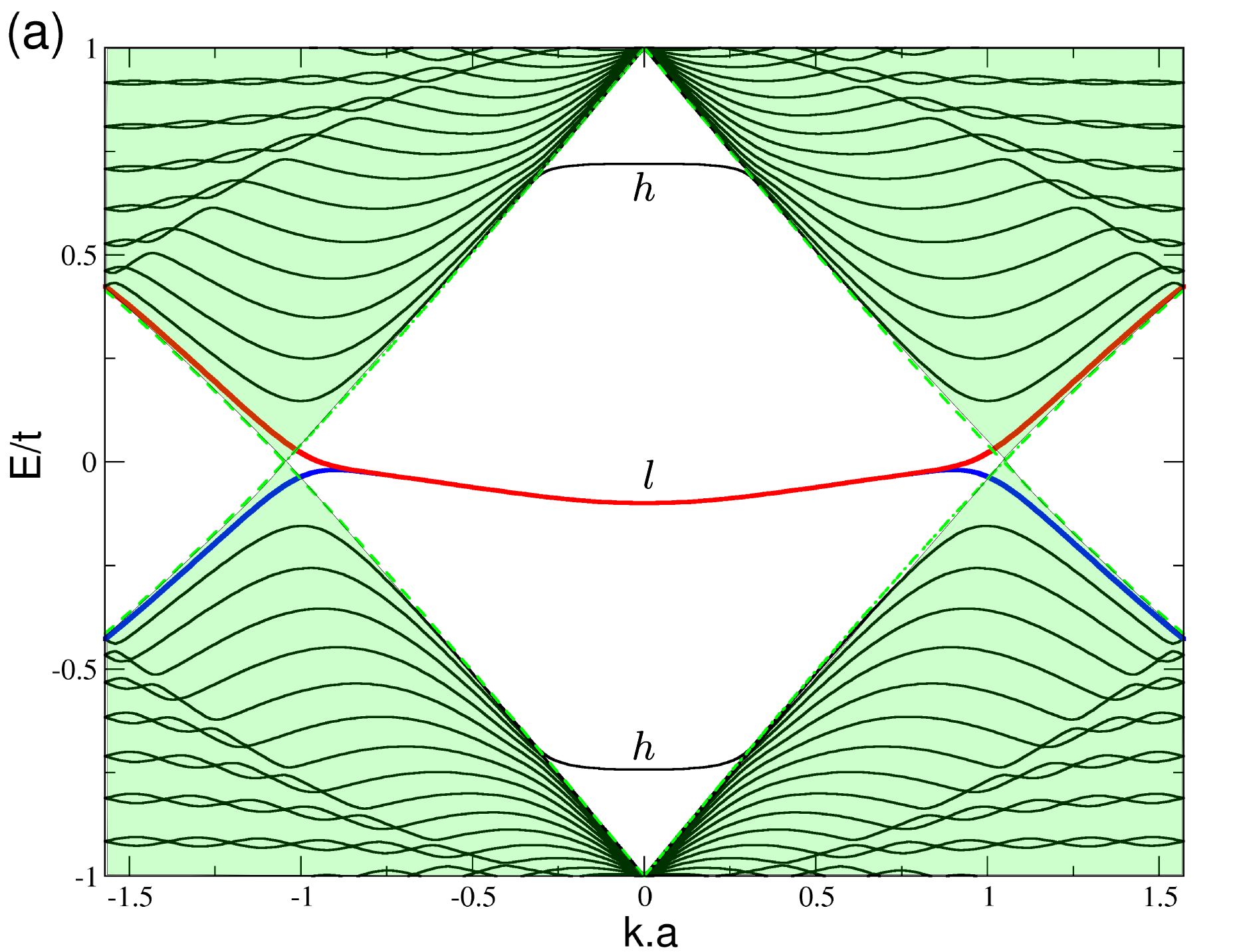
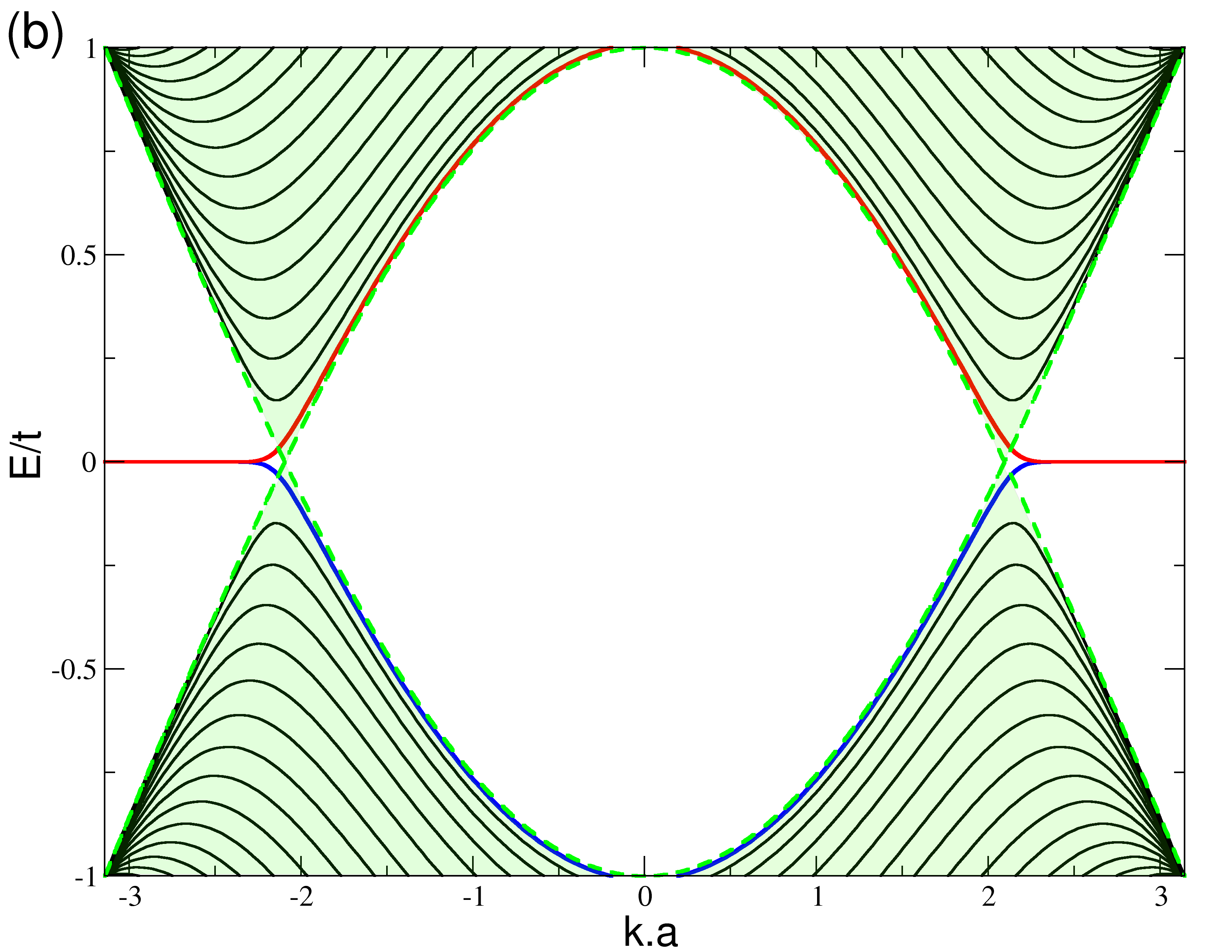
Figure 6: $(a)$: Low-energy spectrum of a ZGNR with $N=30$ and both edges totally reconstructed with SW defects, $zz(57)$. Remember that the energy spectrum of a totally reconstructed edge, results from a doubled unit cell relatively to the pristine ZGNRs, and consequently is double-folded relatively to the latter. The labeled energy levels $(b)$: Low-energy spectrum of a pristine ZGNR with $N=30$ and zigzag edges. Both $(a)$ and $(b)$ were obtained using a tight-binding model. In both cases, the shaded areas indicate which levels are allowed in bulk graphene. Eigenstates corresponding to levels that are outside the shaded region, will necessarily be located at the edges of the ribbon both in $(a)$ $zz(57)$ edges and in $(b)$ perfect zigzag edges. In the $(a)$ panel, the levels labeled by $h$ and $l$, stand, respectively, for high and low-energy.

Since edge states decay exponentially into the bulk, in wide ribbons they can be studied as states of semi-infinite ribbons: states at different edges are uncoupled if the ribbon width is much larger than the decay length. In the case of a semi-infinite ribbon with pristine zigzag edges, the edge states occur at zero-energy.Nakada et al. (1996); Wakabayashi et al. (1999) In such a case, the tight-binding equations simplify to independent recurrence relations for the amplitudes of the $A$ and $B$ sub-lattices, which yield, transparently, the exact wave-functions, the analytical expression of the decay length as function of the momentum along the edge, and the range of momentum values in which such states are possible. In the case of a zigzag ribbon with edges totally reconstructed with SW defects, we face the complication that edge states have dispersion, and are not at zero energy.

To investigate the possibility of low energy edge states of such a system, we must solve the Schrödinger equation,

$$H_{k}|\mu,k\rangle = \epsilon_{\mu,k}|\mu,k\rangle$$ (8)

for $\left|\epsilon_{\mu,k}\right|/t\ll 1$, where $H_{k}$ is the same as that obtained from the transformation in Eq. 7, of the Hamiltonian given by Eqs. (2)-(LABEL:eq:Hbulk) with $n\geq 0$. Note that $H_{k}$ defines effectively a 1D problem in the transverse direction of the ribbon. Consequently, we can express any eigenstate $|\mu,k\rangle$ as a linear combination of the site amplitudes along the transverse direction of the ribbon,

$$|\mu,k\rangle = \sum_{n=0}^{N-1}\sum_{p=1}^{2}\Big{[}A_{p}(k;n)|a;k;p,n\rangle$$ (9)

$$+ B_{p}(k;n)|b;k;p,n\rangle\Big{]},$$

with the one-particle states, $|r;k;p,n\rangle=r_{p}^{\dagger}(k;n)|0\rangle$, where $p=1,2$ and $n=1,\dots,N-1$ define, respectively, the column and the line of the unit cell, and $r=a,b$. To lighten our notation, we have identified the states at the upper edge as

$$|d_{1(4)};k\rangle = |b;k;1(2),1\rangle,$$ (10a)

$$|d_{2(3)};k\rangle = |a;k;1(2),0\rangle,$$ (10b)

$$|c_{1(3)};k\rangle = |a;k;1(2),1\rangle,$$ (10c)

$$|c_{2(4)};k\rangle = |b;k;1(2),2\rangle,$$ (10d)

while at the lower edge

$$|c_{5(7)};k\rangle = |a;k;1(2),N-2\rangle,$$ (11a)

$$|c_{6(8)};k\rangle = |b;k;1(2),N-2\rangle,$$ (11b)

$$|d_{5(8)};k\rangle = |a;k;1(2),N-1\rangle,$$ (11c)

$$|d_{6(7)};k\rangle = |b;k;1(2),N-1\rangle.$$ (11d)

Note that there are four states per zigzag row (identified by $n$), coming from the four sub-lattices $A_{1}$, $B_{1}$, $A_{2}$ and $B_{2}$. Equating coefficients, we obtain a set of $2\times 2\times N$ (tight-binding) equations, where $N$ is the number of zigzag rows of atoms in the unit cell.

To build an analytical description for edge states in a semi-infinite ribbon, with row index $n\geq 0$, we write the TB equations in matrix form, where $\bm{A}(k;n)=\big{[}A_{1}(k;n),A_{2}(k;n)\big{]}^{T}$ and $\bm{B}(k;n)=\big{[}B_{1}(k;n),B_{2}(k;n)\big{]}^{T}$ will stand for column vectors.

For rows with $n>1$, the relations between the amplitudes are the same as those of a pristine ribbon:

$$\mathbf{A}(k;n+1) -W_{A}\mathbf{A}(k;n)=-\left(\frac{\epsilon}{t}\right)\mathbf{B}(k;n+1),$$ (12a)

$$\mathbf{B}(k;n) -W_{B}\mathbf{B}(k;n+1)=-\left(\frac{\epsilon}{t}\right)\mathbf{A}(k;n).$$ (12b)

The matrices $W_{A}$ and $W_{B}$, defined in Eqs. (48), commute and, therefore, share a common eigenbasis, $\{\bm{u^{+}},\bm{u^{-}}\}$ (see Appendix A for details). Let us denote the corresponding eigenvalues by $\xi_{A}^{\pm}$ and $\xi_{B}^{\pm}$, respectively. These quantities depend on the value of the longitudinal momentum, $k$ and are given by:

$$\xi_{A}^{+} = -2\cos(ka/2)e^{i\frac{ka}{2}},$$ (13a)

$$\xi_{A}^{-} = 2i\sin(ka/2)e^{i\frac{ka}{2}},$$ (13b)

$$\xi_{B}^{+} = -2\cos(ka/2)e^{-i\frac{ka}{2}}=\left(\xi_{A}^{+}\right)^{*},$$ (13c)

$$\xi_{B}^{-} = -2i\sin(ka/2)e^{-i\frac{ka}{2}}=\left(\xi_{A}^{-}\right)^{*}.$$ (13d)

Changing to the $\{\bm{u^{+}},\bm{u^{-}}\}$ basis,

$$\bm{A}(k;n) = \alpha_{+}(k;n)\bm{u^{+}}+\alpha_{-}(k;n)\bm{u^{-}},$$ (14a)

$$\bm{B}(k;n) = \beta_{+}(k;n)\bm{u^{+}}+\beta_{-}(k;n)\bm{u^{-}},$$ (14b)

we obtain Eqs. (12) in the form,

$$\alpha_{\sigma}(k;n+1)-\xi_{A}^{\sigma}\alpha_{\sigma}(k;n) =-\left(\frac{\epsilon}{t}\right)\beta_{\sigma}(k;n+1),$$ (15a)

$$\beta_{\sigma}(k;n)-(\xi_{A}^{\sigma})^{*}\beta(k;n+1) =-\left(\frac{\epsilon}{t}\right)\alpha_{\sigma}(k;n),$$ (15b)

where $\sigma=\pm 1$. Note that with the two possible values for $\sigma$, Eqs. (15) give four equations. These equations describe two independent 1D $AB$ chains in the $n$ coordinate, one for each of the modes $\mathbf{u}_{+}$ and $\mathbf{u}_{-}$; the hopping amplitude alternates between $-t$ and $t\xi_{A}^{\sigma}$.

The two modes $\mathbf{u}_{+}$ and $\mathbf{u}_{-}$ are easily interpreted. If we look for propagating solutions ($q_{\sigma}$ real),

$$\alpha_{\sigma}(k;n) =\alpha_{\sigma}(k)e^{iq_{\sigma}n},$$ (16a)

$$\beta_{\sigma}(k;n) =\beta_{\sigma}(k)e^{iq_{\sigma}n},$$ (16b)

we arrive at the equation

$$\left(\frac{\epsilon}{t}\right)^{2}=\left|\left(1-e^{-iq_{\sigma}}\xi_{A}^{\sigma}\right)\right|^{2}.$$ (17)

Low energy states correspond to $(\epsilon/t)^{2}\ll 1$; but it can easily be checked from Eqs. (13), that $\left|\xi_{A}^{+}\right|\geq\sqrt{2}$, for all $ka$ in the F.B.Z., whereas $\left|\xi_{A}^{-}\right|\approx 1$ around $ka=\pm\pi/3$. Hence, propagating states of the $\sigma=+$ modes have an energy of order $t$; the $\sigma=-$ modes are the low energy bulk states when $k$ is near the Dirac value. The existence of these two modes reflects the folding of the Brillouin zone to account for the doubling of the unit cell. At the Bloch momentum of a Dirac point there are two different energy levels, only one of which is of low energy, and corresponds to the $\mathbf{u}_{-}$ mode. In fact, inspecting the relation between the $A_{1}$ and $A_{2}$ amplitudes in the $\mathbf{u}_{-}$mode [see Appendix A, Eqs. (54)] one sees that it corresponds to what is expected from a plane wave at a Dirac point.

Nevertheless, for decaying states $(q_{\sigma}$ with an imaginary part), we cannot exclude the possibility that low energy states can have a $\sigma=+$ component, because in that case, the right hand side of Eq. (17) has a factor $(1-e^{-\Im q_{+}}(\xi_{A}^{+})^{*}e^{i\Re q_{+}})$, which can be close to zero. We will see in a moment that the boundary conditions (BCs) arising from the $zz(57)$ edge bring about precisely this situation.

Let us now discuss what kind of solutions are obtained from Eqs. (15) if the system supports zero energy states. For zero energy, the bulk Eqs. (15) become independent recursion relations

$$\alpha_{\sigma}(k;n+1) = \xi_{A}^{\sigma}\alpha_{\sigma}(k;n),$$ (18a)

$$\beta_{\sigma}(k;n+1) = \frac{1}{\left(\xi_{A}^{\sigma}\right)^{*}}\beta_{\sigma}(k;n).$$ (18b)

From Eqs. (13), $\left|\xi_{A}^{+}\right|>\sqrt{2}$, thus requiring $\alpha_{+}(k,n)=0$, otherwise we would have a non-normalizable state. Also, we must have either $\alpha_{-}(k,n)$ or $\beta_{-}(k,n)=0$, depending on whether $\left|\xi_{A}^{-}\right|$ is greater or smaller than $1.$ Consider, for instance, the latter case: the required conditions for zero energy states would then be $\alpha_{+}(k,n)=\beta_{-}(k,n)=0$.

The previous paragraph did not impose any type of conditions arising from the boundary. It turns out that the existence of zero energy states depends on the specific form of the boundary conditions. We note however, that in this type of edge reconstruction surface states always exist, but not necessarily at zero energy. The boundary conditions can be derived form the tight-binding equations for the rows $n=0,1$. As shown in Appendix A, Eq. (56), they can be approximated by the zero energy BCs, $\bm{\alpha}(k;2)=\mathcal{M}\mathbf{\bm{\beta}}(k;2)$, where $\mathcal{M}$ is a $k$ dependent matrix defined explicitly in Appendix A; in full,

$$\alpha_{+}(k;2) =\mathcal{M}_{++}\beta_{+}(k;2)+\mathcal{M}_{+-}\beta_{-}(k;2),$$ (19a)

$$\alpha_{-}(k;2) =\mathcal{M}_{-+}\beta_{+}(k;2)+\mathcal{M}_{--}\beta_{-}(k;2).$$ (19b)

In the case where zero energy states exist, the boundary conditions defined by Eqs. (19) are exact. For the $k$ values for which $\left|\xi_{A}^{-}\right|<1$, zero energy states require, as we have seen, $\alpha_{+}(k)=\beta_{-}(k)=0$; this is possible only if $\mathcal{M}_{++}=0$. This condition is, in fact, verified in certain limits, the simplest one corresponding to ignoring the hopping renormalizations at the edge, that is, taking $h_{i}=v=h_{i}^{\prime}=1$, in which case the matrix $\mathcal{M}$ reads

$$\mathcal{M}=-4\sin^{2}(ka)\left[\begin{array}[]{cc}0&(\xi_{A}^{-})^{*}\\ (\xi_{A}^{+})^{*}&0\end{array}\right].$$ (20)

Another interesting limit to consider is $h^{\prime}_{i}=1.$ In this case, one obtains

$$\mathcal{M}_{++}\propto h_{1}^{2}-h_{2}h_{4},$$ (21)

and consequently, zero-energy states should be observed if $h_{1}^{2}-h_{2}h_{4}=0.$

We have confirmed these results by numerical diagonalization of the tight-binding Hamiltonian. In both situations, as $\mathcal{M}_{++}=0$, the zero-energy states appear in the range where $\left|\xi_{A}^{-}\right|<1$, i.e., $\left|ka\right|<\pi/3$, and have the form (for $n>1$)

$$\mbox{$\alpha$}_{-}(k;n) = \left(\xi_{A}^{-}\right)^{n-2}\alpha_{-}(k),$$ (22a)

$$\beta_{+}(k;n) = \left(\frac{1}{\left(\xi_{A}^{+}\right)^{*}}\right)^{n-2}\beta_{+}(k),$$ (22b)

with

$$\alpha_{-}(k)=-4\sin^{2}(ka)(\xi_{A}^{+})^{*}\beta_{-}(k).$$ (23)

In Fig. 7 we compare numerical diagonalization results with those of the present analysis, for the simplified situation where hopping renormalizations at the edge are ignored, $h_{i}=v=h_{i}^{\prime}=1$. The squared amplitudes of the edge states, of a narrow ribbon with $N=30$ ($65\mathring{A}$ wide), calculated numerically, are indeed in very good agreement with those of the edge states of a semi-infinite ribbon obtained analytically, from Eqs. (22) and (23).

Unlike the zero energy states occurring in unreconstructed ZGNR, the wave function amplitudes of the edge states are non-zero in both sub-lattices. Those familiar with the Dirac equation description of graphene might find this result surprising, since, at zero energy, the equations for the $A$ and $B$ fields decouple, and only one of them can be non-zero.Brey and Fertig (2006) However, as can be seen in Fig. 7, panels $(a4)$-$(a5)$ – which refer to a value of $k$ close to a Dirac point –, the decay length is much shorter in the $B$ sub-lattice; this is related to the fact that the $B$ amplitudes correspond to the $\sigma=+$ mode, which, in the bulk, is high energy, and has a finite decay length, of the order of a single row width, even at the Dirac point, contrasting with the $\sigma=-$ mode, whose decay length diverges at the Dirac point. So, away from the boundary, the edge state wave function is, in fact, similar to that of a ZGNR, because the amplitude at the $B$ sub-lattice is exponentially smaller than in the $A$ one; but the reconstructed edge requires the presence of the confined $\sigma=+$ mode, in order to satisfy the BC. When we move away from the Dirac point, the distinction between high and low energy modes washes away, and both modes are confined within atomic distances to the edges [Fig. 7, panels $(a2)$-$(a3)$].

Figure 7: $(a)$: ZGNR with two simplified $zz(57)$ edges ($h_{i}=v=h_{i}^{\prime}=1$) and a width of $65\mathring{A}$ (or $N=30$ zigzag lines). The panel $(a1)$ shows the tight-binding low-energy spectrum in the FBZ. The two lowest-energy levels are colored in blue and red. The dashed (orange) horizontal line, signals the position of the Fermi level. Panels $(a2)$ and $(a4)$, show the edge state squared amplitude corresponding to the blue level in $(a1)$, for $ka=0.704$ and $ka=0.842$ respectively (whose position is identified in panel $(a)$ by the vertical dashed green lines). The continuous (dashed) dark blue line stands for the amplitude in the $A_{1}$-sub-lattice ($B_{1}$-sub-lattice) corresponding to the blue level in $(a1)$ obtained from the numerical diagonalization of the TB Hamiltonian (the red level is an identical edge state). Only the amplitudes $A_{1}(k;n)$ and $B_{1}(k;n)$ were plotted, because $A_{2}(k;n)$ and $B_{2}(k;n)$ are identical to the former. The continuous (dashed) light blue line stands for the zero-energy edge state amplitude in the $A_{1}$-sub-lattice ($B_{1}$-sub-lattice) obtained analytically in a semi-infinite ribbon. Note the extreme coincidence between the numerical and the analytical edge states. Panels $(a3)$ and $(a5)$, show the same plots as in $(a2)$ and $(a4)$, but now with logarithmic scale in the $y$-axis, to display the exponential decay of the squared amplitudes. $(b)$: ZGNR with two real $zz(57)$ edges (see Table 1) and a width of $65\mathring{A}$. The panels are organized as those of $(a)$.

At this point we come back to the consideration of real edges, where the hopping parameters have the values in Table 1. One does not find $\mathcal{M}_{++}=0,$ and the BCs of Eqs. (19) are no longer compatible with the conditions for zero energy states, $\alpha_{+}(k)=\beta_{-}(k)=0$, (or $\alpha_{+}(k)=\alpha_{-}(k)=0$, if $\left|\xi_{A}^{-}\right|>1$); edge states, if they exist, have to be dispersive. The dispersiveness of the edge states’ levels can be seen in panel $(b1)$ of Fig. 7.

We analyze this situation in detail in Appendix B. If a semi-infinite 1D $AB$ chain has a zero energy edge state with BC, say $B(0)=0$, it will still have a low but finite energy one, if the BC is replaced by $B(0)=sA(0)$ with $\left|s\right|<1.$ In the present case the situation is more complex, because the problem involves two 1D chains [Eqs. (15)], coupled by the BC [Eq. (19)]. The main conclusion still holds, and we expect low energy, dispersive, edge states near the Dirac points ($ka=\pm\pi/3$).

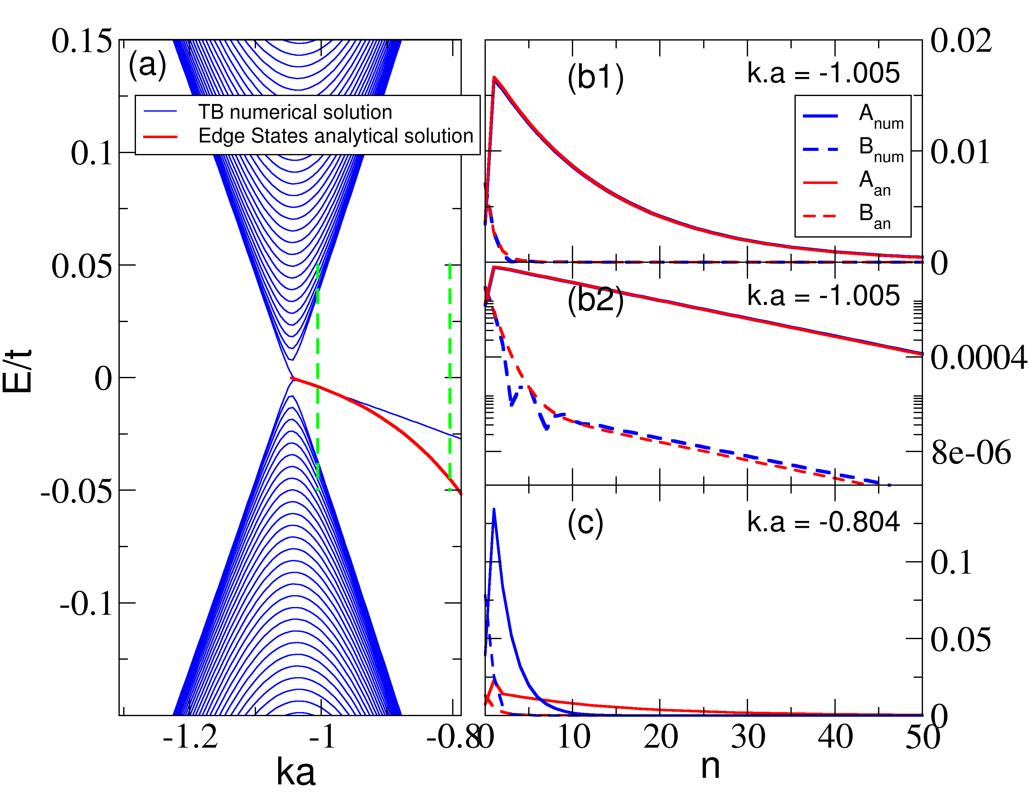
Figure 8: Comparison between the edge state levels obtained from numerical diagonalizing the tight-binding Hamiltonian of a ribbon with $N=600$ ($\approx 900\mathring{A}$ wide) (in blue), and the edge state level resulting from analytically solving the TB equations, by using simplified (zero-energy) BCs (in red). $(a)$ shows the energy as function of $k$; panels $(b1)$ and $(c)$, show the square of the amplitudes as function of distance to the edge, for $ka=-1.005$ and $ka=-0.804$ respectively. These values of $ka$ are identified in panel $(a)$ by vertical green dashed lines; $(b2)$ panel is the same as $(b1)$, but now in logarithmic scale.

In Fig. 8 we compare analytical results for a semi-infinite chain, obtained with the procedure described in Appendix B, with numerical diagonalization of a very wide ribbon ($N=600$). The use of the zero energy BC of Eq. (19) correctly accounts for the wave function and for the energy dispersion as a function of $k$, but only very close to the Dirac point. It quickly deviates strongly from the numerical results as we move away from the Dirac point. This is to be expected, not only as a result of the violation of the low energy condition, but, more importantly, because the description in terms of bulk equations and simplified BCs will not hold when the edge state has such a short decay length that it lives mostly at the edge. Moreover, as stated before, near the Dirac points the localization length of the mode $\sigma=-$ diverges. As a consequence, the analytical analysis developed in Appendix B, will only accurately describe the physics of $zz(57)$ edged ribbons near the Dirac points if the ribbons are large.

We can summarize the results of this subsection, saying that, as a consequence of the duplication of the unit cell, Stone-Wales reconstructed edges present a new type of edge state,

$$\mathbf{A}(k;n) =e^{iq_{+}(n-2)}\alpha_{+}\mathbf{u}_{+}+\alpha_{-}e^{iq_{-}(n-2)}\mathbf{u}_{-},$$ (24)

$$\mathbf{B}(k;n) =e^{iq_{+}(n-2)}\beta_{+}\mathbf{u}_{+}+\beta_{+}e^{iq_{-}(n-2)}\mathbf{u}_{-},$$ (25)

with the following features: (i) the states are dispersive; (ii) the wave-function, even for the semi-infinite ribbon, has non-zero amplitudes on both sub-lattices; (iii) close to $k=\pm\pi/3$, the Dirac points, the wave function amplitudes have two components decaying with very different rates, $\Im q_{-}$ and $\Im q_{+}$, the latter remaining finite even at the Dirac point, and corresponding to a mode with only atomic scale penetration into the bulk.

This last feature is strikingly apparent in Fig. 8, panel $(b2)$, where the faster decaying component in the $B$ lattice dominates the wave function close to the edge, because of a larger initial amplitude, $\left|\beta_{+}\right|\gg\left|\beta_{-}\right|$, but is supplanted by the one with slower decay, around $n\approx 10$.

II.4 Perpendicular magnetic field

When a perpendicular magnetic field is applied to a graphene sheet, electrons acquire a cyclotron motion, with quantized cyclotron radius and macroscopically degenerate energy levels, the so called Landau levels (LL). In a ribbon, LL degeneracy is partially lifted, because the edges interrupt the cyclotron orbits located close to them. In this section we discuss the effect of a perpendicular magnetic field in the low energy spectrum of the tight-binding models we have been discussing (a ribbon with a $zz(57)$ reconstruction).

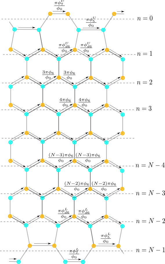
Figure 9: Peierls phases of a zigzag ribbon with totally reconstructed edges ($N=10$).

The introduction of a static magnetic field, applied perpendicularly to the ribbon, $\bm{B}=B\bm{\hat{e}_{z}}$, can be achieved by a Peierls substitution of the hopping integrals,Peierls (1933); Boykin et al. (2001)

$$t_{ij} \to t_{ij}e^{i2\pi\phi_{ij}},$$ (26)

where $t_{ij}$ stands for the hopping integral between the position $\bm{R_{i}}$ and the position $\bm{R_{j}}$ in the absence of a magnetic field, and the phase $\phi_{ij}$ is given by the line integral

$$\phi_{ij} = \frac{1}{\phi_{0}}\int_{\bm{R}_{i}}^{\bm{R}_{j}}\bm{A}\cdot\textrm{d}\bm{r},$$ (27)

where $\bm{A}$ is the potential vector and $\phi_{0}=h/e$ is the flux quantum. Note that the magnetic flux through the area $\Sigma$, in units of the flux quantum $\phi_{0}$, is

$$\frac{1}{\phi_{0}}\int_{\Sigma}\textrm{d}\bm{\sigma}\cdot\bm{B} = \frac{1}{\phi_{0}}\oint\textrm{d}\bm{r}\cdot\bm{A}=\sum_{\mathrm{around}\textrm{ }\Sigma}\phi_{ij}.$$ (28)

The zigzag edge reconstruction modifies, not only the hoppings, but also the areas of the pentagons, heptagons and hexagons near the edge. Therefore, by Eq. (27), the Peierls phases around the edges are distinct from those in the ribbon bulk. We choose a gauge that yields Peierls’ phases as shown in Fig. 9, clearly satisfying Eq. (28), $\phi_{6}$ being the magnetic flux per hexagon in the bulk graphene lattice.

The spectrum shown in Fig. 10$(a)$ is essentially the same as for a pristine ZGNR (apart from the folding of the Brillouin zone), the most prominent feature being a doubly degenerate zero energy level occurring between the two Dirac points. But what is displayed is, in fact, the spectrum of a ribbon with simplified $zz(57)$ edges, where hopping renormalizations were ignored ($h_{i}=1$, $v_{i}=1$), and the pentagons and heptagons considered to have the same area as all the hexagons.

Figure 10: Panel $(a)$ shows the tight-binding energy spectrum of a zigzag graphene nanoribbon with simplified $zz(57)$ edges ($h_{i}=v=h^{\prime}_{i}=1$ and $\phi_{5}^{C}=\phi_{7}^{C}=2\phi_{\textrm{d}6}^{C}=2\phi_{6}$) with a width of $214\mathring{A}$ (or $N=100$ zigzag rows) in the presence of a perpendicular magnetic field, $B=80T$. The green dashed vertical lines in $(a)$, indicate the different values of $ka$ for which the edge states were plotted in $(b)$-$(p)$. Panels $(b)$-$(p)$ show in dark blue, for different values of $ka$, the wave function squared modulus of the two lowest-energy levels highlighted in panel $(a)$ with blue and red fill. The light blue curves in panels $(f)$-$(o)$ stand for the edge states obtained analytically for values of $ka$ for which their energy is zero [see panel $(a)$].

In Fig. 11$(a)$, we display the spectrum of a zigzag ribbon with real $zz(57)$ edges in the presence of a perpendicular magnetic field. In contrast with the previous case, the two zero-energy levels are now split in energy and dispersive, crossing each other at the $\Gamma$-point.

Figure 11: Panel $(a)$ shows the tight-binding energy spectrum of a zigzag graphene nanoribbon with real $zz(57)$ edges with a width of $214\mathring{A}$ (or $N=100$ zigzag rows) in the presence of a perpendicular magnetic field, $B=80T$. Panels $(b)$-$(p)$ show the squared modulus of the lowest-energy levels wave functions for different values of $ka$ [blue and red levels in panel $(a)$]. The green dashed vertical lines in $(a)$, indicate the different values of $ka$ for which the edge states wave functions squared modulus were plotted in $(b)$-$(p)$.

The plots of the wave functions suggest a clear interpretation of this result. In graphene there is a bulk zero energy LL which cannot be affected by BCs, because the corresponding wave functions are localized in the bulk and do not reach the edges. And, in fact, one can see in Fig. 11$(a)$ regions of $k$ with a flat energy level at zero energy; the plots of the corresponding wave functions ($-0.9\lesssim ka\lesssim-0.5$ and $1.2\lesssim ka\lesssim 1.5$) show one localized state inside the ribbon. The remaining states are edge states localized at its boundaries. In a real reconstructed edge, these states are dispersive in zero magnetic field, as we have seen in the previous section, and remain dispersive in a magnetic field: hence the lifting of the degeneracy and the level crossing at the $\Gamma$ point, which involves states localized at opposite edges. On the other hand, in the simplified $zz(57)$ ribbon, the edge states occur at zero energy, as we have also seen. So the doubly degenerate zero energy state is either a zero energy bulk LL and an edge state, or two edge states, located at opposite ends of the ribbon. This is confirmed by the plots of the wave functions.

We now proceed to indicate briefly how these results arise from the Peierls substitution. We begin by considering the appearance of a zero energy bulk Landau level (BLL). The recurrence relations for the amplitudes now involve matrices that depend on the row index,

$$\bm{A}(k;n+1) = \widetilde{W}_{A}(n)\bm{A}(k;n),$$ (29a)

$$\bm{B}(k;n+1) = \widetilde{W}_{B}^{-1}(n+1)\bm{B}(k;n).$$ (29b)

Recall that $\bm{A}(k;n)$ and $\bm{B}(k;n)$ are notations for the column vectors, $\bm{A}(k;n)=\big{[}A_{1}(k;n),A_{2}(k;n)\big{]}^{T}$ and $\bm{B}(k;n)=\big{[}B_{1}(k;n),B_{2}(k;n)\big{]}^{T}$; the matrices $\widetilde{W}_{A}(n)$ and $\widetilde{W}_{B}(n)$ are written in Appendix C. As before, these are commuting matrices, and have the common basis $\{\mathbf{u_{+}},$$\mathbf{u}_{-}\}$; the eigenvalues, however, depend on the row index,

$$\widetilde{\xi_{A}^{+}}(r) = -2e^{ika/2}\cos\left[\frac{ka}{2}-(r+1)\pi\frac{\phi_{6}}{\phi_{0}}\right]=\left(\widetilde{\xi_{B}^{+}}(r)\right)^{*},$$

$$\widetilde{\xi_{A}^{-}}(r) = 2ie^{ika/2}\sin\left[\frac{ka}{2}-(r+1)\pi\frac{\phi_{6}}{\phi_{0}}\right]=\left(\widetilde{\xi_{B}^{-}}(r)\right)^{*}.$$

We can then rewrite Eqs. (29), for $m\geq 2,$ as

$$\bm{A}(k;n) = \Xi_{A}^{+}(n,m)\alpha_{+}(k;m)\bm{u^{+}}$$ (31a)

$$+ \Xi_{A}^{-}(n,m)\alpha_{-}(k;m)\bm{u^{-}},$$

$$\bm{B}(k;n) = \Xi_{B}^{+}(n,m)\beta_{+}(k;m)\bm{u^{+}}$$ (31b)

$$+ \Xi_{B}^{-}(n,m)\beta_{-}(k;m)\bm{u^{-}},$$

where $n\geq m$, $\alpha_{\sigma}$ and $\beta_{\sigma}$ are undetermined coefficients, while the quantities $\Xi_{A}^{\pm}(n,m)$ and $\Xi_{B}^{\pm}(n,m)$ are a shorthand for

$$\Xi_{A}^{\sigma}(n,m) = \prod_{r=m}^{n-1}\widetilde{\xi_{A}^{\sigma}}(r),$$ (32a)

$$\Xi_{B}^{\sigma}(n,m) = \prod_{r=m+1}^{n}\frac{1}{\widetilde{\xi_{B}^{\sigma}}(r)}.$$ (32b)

As a function of the row index $n$, $\Xi_{A(B)}^{\sigma}(n,m)$ goes through a maximum when $\left|\widetilde{\xi_{A}^{\sigma}}(r)\right|\left(\left|\widetilde{\xi_{B}^{\sigma}}(r)\right|^{-1}\right)$ decreases below 1. These maxima are repeated periodically when $n$ changes by $2n_{\phi}$, where $n_{\phi}\equiv\phi_{0}/\phi_{6}$ is the number of hexagons required for a total flux equal to a flux quantum. These multiple maxima are related to commensurability effects between the lattice parameter and the cyclotron radius and are only important for unrealistically high fields. Thouless et al. (1982) For achievable values of the magnetic field, $n_{\phi}$ is much larger than the ribbon width, $N$, (for $B=80\,\mathsf{T}$, $2n_{\phi}\approx 2000$), and at most one maximum of $\Xi_{A(B)}^{\sigma}(n,m)$ is located inside the ribbon, as shown in Fig. 12. Assume, for instance, that that is the case for $\Xi_{B}^{-}$ at

$$\bar{n}_{B-} =\frac{ka}{2\pi}n_{\phi}-\left(\frac{5}{6}+q\right)n_{\phi},\qquad 1\ll\bar{n}_{B-}\ll N-1,$$ (33a)

$$\bar{n}_{A+} =\frac{ka}{2\pi}n_{\phi}-\left(\frac{2}{3}+q\right)n_{\phi}=\bar{n}_{B-}+\frac{n_{\phi}}{6},$$ (33b)

$$\bar{n}_{A-} =\frac{ka}{2\pi}n_{\phi}-\left(\frac{1}{6}+q\right)n_{\phi}=\bar{n}_{B-}+\frac{2n_{\phi}}{3},$$ (33c)

$$\bar{n}_{B+} =\frac{ka}{2\pi}n_{\phi}-\left(\frac{1}{3}+q\right)n_{\phi}=\bar{n}_{B-}+\frac{n_{\phi}}{2},$$ (33d)

where $q$ is an integer. From Eqs. (33), we conclude that for reasonable values of the magnetic field and ribbon widths, at most, only one of the components will have a maximum inside the ribbon (of width $N=100$). See, as an example, Fig. 12.

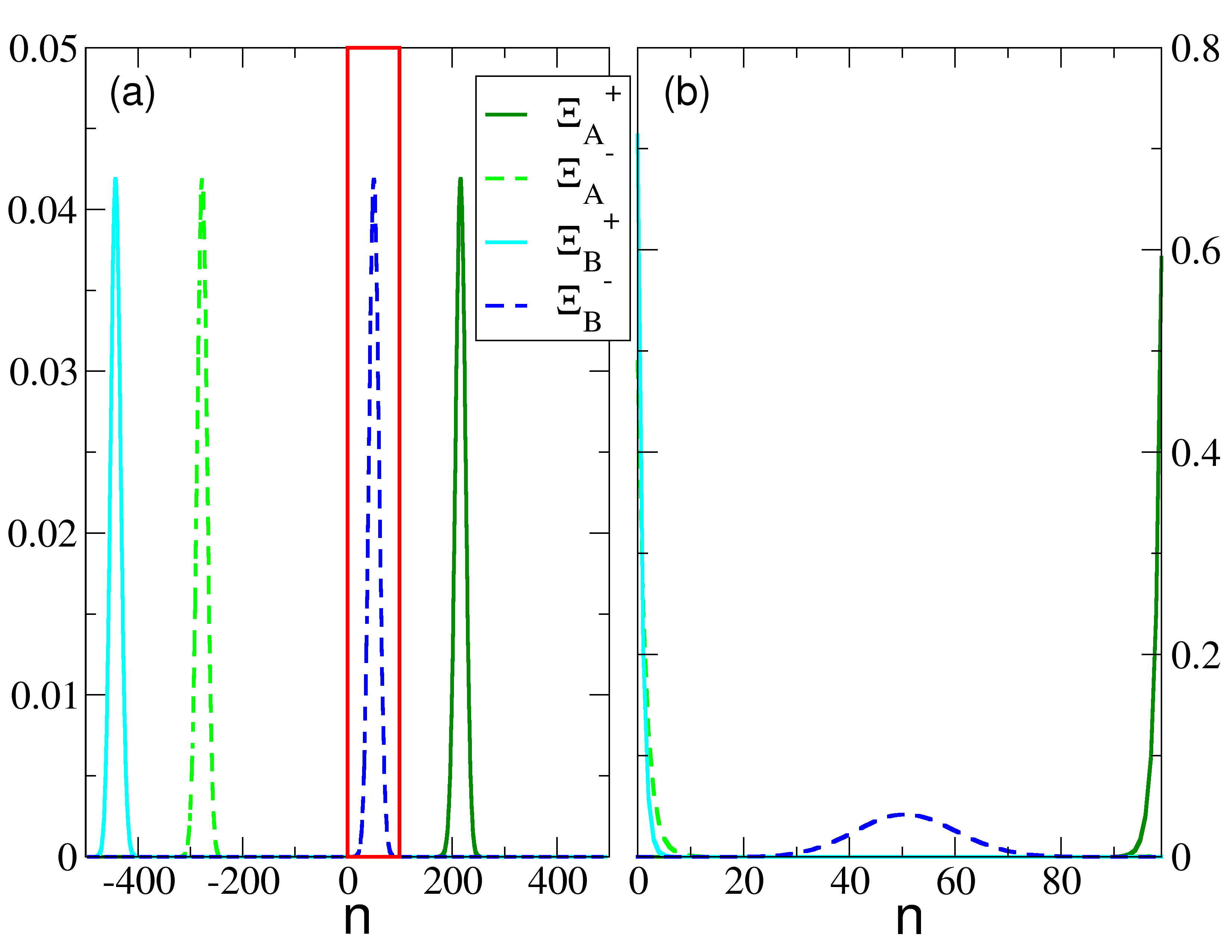
Figure 12: Plot of $|\Xi_{A}^{\pm}(n)|$ and $|\Xi_{B}^{\pm}(n)|$ (that can be interpreted as the amplitudes of the four components of the wave function in the proper basis of the matrices $\widetilde{W}$), given by Eqs. (32). The above quantities were plotted for $B=80T$ and $ka=-0.716$. In the $(a)$ panel, the $|\Xi_{A/B}^{\pm}(n)|$ are normalized over the region $n\in[-500,500]$, while in the $(b)$ panel they are normalized over $n\in[0,100]$. The red box in panel $(a)$ signals the region where $n\in[0,100]$.

Moreover, the amplitude $\beta_{-}(k,n)$ will decay exponentially to very small values at the edges; to exponential accuracy, the BCs, whatever they may be, are trivially satisfied by choosing $\alpha_{+}=\alpha_{-}=\beta_{+}=0$; this then is a BLL, where the wave function exists only in one of the sub-lattices and is localized away from the edges. These BLLs occur irrespective of the type of edge. However, when $k$ changes and the LL center approaches the edge, the BCs come into play, differentiating the various situations.

Let us now consider the appearance of the edge states in these results. The general BC for a reconstructed zigzag edge with SW defects at the $n=0$ end, may be written as $\bm{\alpha}(k;2)=\widetilde{\mathcal{M}}\mathbf{\bm{\beta}}(k;2)$, where $\widetilde{\mathcal{M}}$ is defined in Appendix C, Eq. (70), with an analogous expression for the edge in $n=N-1$, $\mathbf{\bm{\beta}}(k;N-3)=\widetilde{\mathcal{M}}^{\prime}\bm{\alpha}(k;N-3)$.

We will start by assuming that the ribbon is terminated with a simplified $zz(57)$ edge ($h_{i}=v=h_{i}^{\prime}=1$ and $\phi_{7}=\phi_{5}=2\phi_{d6}=2\phi_{6}$). In such a situation, we have $\widetilde{\mathcal{M}}_{++}=\widetilde{\mathcal{M}}_{--}=0$, a result which uncouples the components $\alpha_{+}$ and $\beta_{-}$ from $\alpha_{-}$ and $\beta_{+}$

$$\alpha_{+}(k;2) = \widetilde{\mathcal{M}}_{+-}\beta_{-}(k;2),$$ (34a)

$$\alpha_{-}(k;2) = \widetilde{\mathcal{M}}_{-+}\beta_{+}(k;2).$$ (34b)

As a consequence, every time we have a zero energy BLL (living away from the edges), we will also have one other solution of zero energy, now localized at the edge. Let us take as an example, the case where $ka=-0.716$, for which the $\Xi_{A/B}^{\pm}$ are depicted in Fig. (12). To exponential accuracy, the BCs involving $\beta_{-}$ and $\alpha_{+}$ are trivially satisfied at both edges choosing $\alpha_{+}=0$. Those involving $\beta_{+}$ and $\alpha_{-}$, are satisfied at the upper edge choosing $\alpha_{-}(k;2)=\widetilde{\mathcal{M}}_{-+}\beta_{+}(k;2)$, being satisfied at the lower edge to exponential accuracy. In the real space [see Eqs. (31)], we will have a BLL localized only on the $B$ sub-lattice and an edge state around the edge at $n=0$, living in both sub-lattices with different localization lengths.

When the value of $ka$ is increased, the maxima of $\Xi_{A/B}^{\pm}$ move to higher values of $n$. At a certain point, the maximum of $\Xi_{B}^{-}$ will be such that $\bar{n}_{B-}>N-1$, and then there will be no maxima inside the ribbon. In such a case, the maxima of $\Xi_{B}^{-}$ and $\Xi_{A}^{+}$ closer to the ribbon, will be at $n>N-1$, while the maxima of $\Xi_{B}^{+}$ and $\Xi_{A}^{-}$ closer to the ribbon, will be at $n<0$. In this case, the BCs involving $\beta_{-}$ and $\alpha_{+}$ will be satisfied at the lower edge choosing $\beta_{-}(k;N-3)=\widetilde{\mathcal{M}}^{\prime}_{-+}\alpha_{+}(k;N-3)$. At the upper edge, the BC will be obeyed to exponential accuracy. The converse needs to be done regarding the BCs involving $\beta_{+}$ and $\alpha_{-}$. Consequently, for $-0.5\lesssim ka\lesssim 1.2$, there will be zero-energy solutions localized at both edges, living in both sub-lattices with distinct localization lengths in each sub-lattice.

If, on the contrary, we start decreasing the value of $ka$ from $ka\approx-0.72$, the maxima of $\Xi_{A/B}^{\pm}$ moves to lower values of $n$, and at a certain point, the maximum of $\Xi_{B}^{-}$ will be such that $\bar{n}_{B-}<0$. In such case, the maxima of $\Xi_{B}^{-}$ and $\Xi_{A}^{-}$ closer to the ribbon, will be at $n<0$, while the maxima of $\Xi_{B}^{+}$ and $\Xi_{A}^{+}$ closer to the ribbon, will be at $n>N-1$. In this case, it will not be possible to satisfy the BCs non-trivially and consequently, there will be no zero-energy solutions in this region, as can be seen in Fig. 10$(a)$.

When instead of simplified $zz(57)$ edges, the ribbon is terminated with real $zz(57)$ edges, the matrix $\widetilde{\mathcal{M}}$ is modified, and $\widetilde{\mathcal{M}}_{++}\neq\widetilde{\mathcal{M}}_{--}\neq 0$, resulting in a BC coupling all the components $\alpha_{\pm}$ and $\beta_{\pm}$

$$\alpha_{+}(k;2) = \widetilde{\mathcal{M}}_{++}\beta_{+}(k;2)+\widetilde{\mathcal{M}}_{+-}\beta_{-}(k;2),$$ (35a)

$$\alpha_{-}(k;2) = \widetilde{\mathcal{M}}_{-+}\beta_{+}(k;2)+\widetilde{\mathcal{M}}_{--}\beta_{-}(k;2).$$ (35b)

To grasp the implications of this modification, consider for instance the case where $ka=-0.716$, depicted in Fig. 12, where a BLL is present in the $\beta_{-}$ mode; since $\beta_{-}(2)\approx 0,$ the BC imply all three remaining amplitudes, $\alpha_{+},\,\alpha_{-}$and $\beta_{+}$ to be non zero, if there is to be an edge state in addition to the BLL. But the $\alpha_{+}$ mode grows as $n$ increases, whereas the other two decrease; as a result the BCs will be violated at the opposing edge. In conclusion, BCs can no longer be satisfied with zero energy edge states, which become dispersive, whereas zero energy BLL still occur. This accounts for the lack of zero energy doubly degenerate state in ribbons with real reconstructed $zz(57)$ edges.

III Conclusion

We have discussed in detail the effect of edge reconstruction on the characteristics of low energy edge states in graphene ribbons. In the case of Stone-Wales $zz(57)$ reconstructed zigzag edges, we find a new type of edge state originating from the doubling of the unit cell along the edge, brought about by the edge reconstruction. This new type of edge state has the following features: (i) the states are in general dispersive, although specific values of the tight-binding model parameters allow zero energy states; (ii) the wave-function, even for the semi-infinite ribbon, has non-zero amplitudes on both sub-lattices; (iii) close to the Dirac points, the wave function amplitudes have two components decreasing with the distance from edge with different decay lengths, one of which remains finite, of the order of the lattice parameter, even at the Dirac point, while the other diverges. The dispersion of the edge states should lead to a charge transfer between bulk and edges (self-doping), which, for realistic values of the tight-binding parameters, leaves the edges negatively charged.

In the presence of a magnetic field, one still finds zero energy bulk Landau Levels, as was to be expected, since these are insensitive to the edges; however, in contrast to pristine zigzag ribbons, where the zero energy LL is degenerate with an edge state, this in no longer true in ribbons with reconstructed edges, since the edge states are, in general, dispersive.

Appendix A Tight Binding equations and boundary conditions

In this appendix, we write the tight-binding equations for the amplitudes at the sites near one edge, $n=0$; these will determine the boundary conditions (BCs) that must be satisfied by the bulk solutions. For clarity, we begin by considering zero energy states. We will argue that the BCs adequate for low energy states, $\left|\epsilon/t\right|\ll 1$, are the same as for zero energy states.

The tight-binding equations at the sites of $A_{1}(m,0)$ and $A_{2}(m,0)$ have the form:

$$h_{2}A_{2}(m;0)+h_{1}B_{1}(m;0) = 0,$$ (36a)

$$h_{2}A_{1}(m,0)+h_{1}B_{2}(m;0) = 0.$$ (36b)

It will be useful to express these in matrix form; after Fourier transforming in the $m$ index, ($k$ is the wave vector along the edge),

$$\mathbf{A}(k;0)=-\frac{h_{1}}{h_{2}}\sigma_{x}\mathbf{B}(k;0),$$ (37)

where $\sigma_{x}$ is a Pauli matrix. For the $B_{1}(m;0),\,B_{2}(m;0)$ sites,

$$h_{4}B_{2}(m-1;0)+h_{1}A_{1}(m;0)+vA_{1}(m;1) =0,$$ (38a)

$$h_{4}B_{1}(m+1;0)+h_{1}A_{2}(m;0)+vA_{2}(m;1) =0.$$ (38b)

Using Bloch’s theorem, we can cast this in the form

$$\mathbf{A}(k;1) +\frac{h_{1}}{v}\mathbf{A}(k;0)$$

$$+\frac{h_{4}}{v}\left[\begin{array}[]{cc}e^{-2ika}&0\\ 0&e^{2ika}\end{array}\right]\sigma_{x}\mathbf{B}(k;0)=0.$$ (41)

Using Eq. (37) in this one,

$$\mathbf{A}(k;1)+\mathcal{R}\sigma_{x}\mathbf{B}(k;0)=0,$$ (42)

where

$$\mathcal{R}:=-\left[\begin{array}[]{cc}\frac{h_{1}^{2}-h_{2}h_{4}e^{-2ika}}{h_{2}v}&0\\ 0&\frac{h_{1}^{2}-h_{2}h_{4}e^{2ika}}{h_{2}v}\end{array}\right],$$ (43)

is a matrix that depends on $k$.

With a similar procedure for the sites $A_{1}(m;1)$, $A_{2}(m;1)$, $B_{1}(m;1)$ and $B_{2}(m,1)$, we obtain

$$\mathbf{A}(k;2) = \mathcal{W}_{A}\mathbf{A}(k;1),$$ (44a)

$$\mathbf{B}(k;0) = \mathcal{W}_{B}\mathbf{B}(k;1),$$ (44b)

with

$$\mathcal{W}_{A}= -\left[\begin{array}[]{cc}h^{\prime}_{1}&h^{\prime}_{1}\\ h^{\prime}_{3}e^{2ika}&h^{\prime}_{3}\end{array}\right],$$ (45c)

$$\mathcal{W}_{B}= -\frac{1}{v}\left[\begin{array}[]{cc}h^{\prime}_{1}&h^{\prime}_{3}e^{-2ika}\\ h^{\prime}_{1}&h^{\prime}_{3}\end{array}\right];$$ (45f)

using Eqs. (42), we arrive at

$$\mathbf{A}(k;2)+\mathcal{W}_{A}\mathcal{R}\sigma_{x}\mathcal{W}_{B}\mathbf{B}(k;1)=0.$$ (46)

Beyond the first row ($n>1$), it is simple to get

$$\mathbf{A}(k;n+1) = W_{A}\mathbf{A}(k,n),$$ (47a)

$$\mathbf{B}(k;n+1) = W_{B}^{-1}\mathbf{B}(k,n),$$ (47b)

where

$$W_{A} = -\left[\begin{array}[]{cc}1&1\\ e^{2ika}&1\end{array}\right],$$ (48c)

$$W_{B} = -\left[\begin{array}[]{cc}1&e^{-2ika}\\ 1&1\end{array}\right],$$ (48f)

In summary, after Fourier transforming in the $m$ variable, the tight-binding equations for a semi-infinite ribbon with $zz(57)$ reconstruction are ($n>1$)

$$\mathbf{A}(k;2) = -\mathcal{W}_{A}\mathcal{R}\sigma_{x}\mathcal{W}_{B}W_{B}\mathbf{B}(k;2),$$ (49a)

$$\mathbf{A}(k;n+1) = W_{A}\mathbf{A}(k,n),$$ (49b)

$$\mathbf{B}(k;n+1) = W_{B}^{-1}\mathbf{B}(k,n).$$ (49c)

The last two are the bulk recursion relations, while the first one contains the BC.

We now generalize these equations for states of finite, but low, energy. We argue that only the bulk equations are changed, the BCs remain the same, i.e.,

$$\mathbf{A}(k;2) =-\mathcal{W}_{A}\mathcal{R}\sigma_{x}\mathcal{W}_{B}W_{B}\mathbf{B}(k;2),$$ (50a)

$$\mathbf{A}(k,n+1) -W_{A}\mathbf{A}(k,n)=-\left(\frac{\epsilon}{t}\right)\mathbf{B}(k,n+1),$$ (50b)

$$\mathbf{B}(k,n) -W_{B}\mathbf{B}(k,n+1)=-\left(\frac{\epsilon}{t}\right)\mathbf{A}(k,n).$$ (50c)

Let us put back the energy in the equations for the amplitudes near the edge,

$$h_{2}A_{2}(m;0)+h_{1}B_{1}(m;0) =-\left(\frac{\epsilon}{t}\right)A_{1}(m;0),$$ (51a)

$$h_{2}A_{1}(m,0)+h_{1}B_{2}(m;0) =-\left(\frac{\epsilon}{t}\right)A_{2}(m;0),$$ (51b)

so Eq.(37) becomes,

$$\mathbf{A}(m;0)+\frac{h_{1}}{h_{2}}\sigma_{x}\mathbf{B}(m;0)=\frac{1}{h_{2}}\left(-\frac{\epsilon}{t}\right)\sigma_{x}\mathbf{A}(m;0).$$ (52)

This shows the pattern that we have to repeat in Eqs. (38) through to Eqs. (44). Instead of Eq. (50a), we obtain,

$$\mathbf{A}(k;2)+ \mathcal{W}_{A}\mathcal{R}\sigma_{x}\mathcal{W}_{B}W_{B}\mathbf{B}(k;2)$$

$$=\left(-\frac{\epsilon}{t}\right) \left[\frac{1}{v}\mathcal{W}_{A}\mathbf{B}(k;0)-\frac{h_{1}}{h_{2}v}\mathcal{W}_{A}\sigma_{x}\mathbf{A}(k;0)\right.$$

$$- \left.\frac{1}{v}\mathcal{W}_{A}\mathcal{R}\sigma_{x}\mathbf{A}(k;1)+\mathbf{B}(k,1)\right].$$ (53)

Naturally, this reduces to Eq. (50a) if the right hand side is set to zero. The important point is that, for the values of the parameters listed in Table 1, the matrix $\mathcal{W}_{A}\mathcal{R}\sigma_{x}\mathcal{W}_{B}W_{B}$ has one finite eigenvalue in the entire range of $k$, whose modulus is always larger than about 1.3. This means that, to lowest order in $\left(-\epsilon/t\right)$, we are justified in neglecting the RHS of this equation, and use the same BC as for zero energy states. This is a valid approximation for states with $\left|\epsilon/t\right|\ll 1$.

Now we change basis to rewrite these equations in the eigenbasis of $W_{A}$ and $W_{B}$, [see Eqs. (14)]

$$\mathbf{u}^{+} = \frac{1}{\sqrt{2}}\left[\begin{array}[]{c}e^{-ika}\\ 1\end{array}\right],$$ (54c)

$$\mathbf{u}^{-} = \frac{1}{\sqrt{2}}\left[\begin{array}[]{c}-e^{-ika}\\ 1\end{array}\right].$$ (54f)

The coordinate transformation is defined by the matrix $U$ given by

$$U=\frac{1}{\sqrt{2}}\left[\begin{array}[]{cc}e^{ika}&1\\ -e^{ika}&1\end{array}\right].$$ (55)

The BC in the new basis, becomes

$$\bm{\alpha}(k;2) =-U\mathcal{W}_{A}\mathcal{R}\sigma_{x}\mathcal{W}_{B}W_{B}U^{\dagger}\bm{\beta}(k;2)$$

$$=\mathcal{M}(k)\bm{\beta}(k;2).$$ (56)

and the bulk equations,

$$\alpha_{\sigma}(k;n+1)-\xi_{A}^{\sigma}\alpha_{\sigma}(k;n) =-\left(\frac{\epsilon}{t}\right)\beta_{\sigma}(k;n+1),$$ (57a)

$$\beta_{\sigma}(k;n)-(\xi_{A}^{\sigma})^{*}\beta(k;n+1) =-\left(\frac{\epsilon}{t}\right)\alpha_{\sigma}(k;n).$$ (57b)

The matrix $\mathcal{M}(k)$ can be calculated explicitly, since all the matrices intervening in its definition were given above, but its long expression is not particularly enlightening.

Appendix B The low-energy edge states

We now sketch the calculation of the low energy edge states for the problem set by Eqs.(50) in a semi-infinite ribbon. For solutions that decay away from the edge,

$$\alpha_{\sigma}(k;n) =e^{iq_{\sigma}(n-2)}\alpha_{\sigma}(k;q_{\sigma}),$$ (58a)

$$\beta_{\sigma}(k;n) =e^{iq_{\sigma}(n-2)}\beta_{\sigma}(k;q_{\sigma}),$$ (58b)

the equations for the amplitudes in the bulk become

$$(1-e^{-iq_{\sigma}}\xi_{A}^{\sigma})\alpha_{\sigma}(k;q^{\sigma}) =-\left(\frac{\epsilon}{t}\right)\beta_{\sigma}(k;q_{\sigma}),$$ (59a)

$$(1-e^{iq_{\sigma}}(\xi_{A}^{\sigma})^{*})\beta_{\sigma}(k;q^{\sigma}) =-\left(\frac{\epsilon}{t}\right)\alpha_{\sigma}(k;q_{\sigma}).$$ (59b)

The energy must be given by

$$\left(\frac{\epsilon}{t}\right)^{2} =\left(1-e^{-iq_{\sigma}}\xi_{A}^{\sigma}\right)\left(1-e^{+iq_{\sigma}}(\xi_{A}^{\sigma})^{*}\right).$$ (60)

Expanding the RHS, and given the fact that the energy must be real, we conclude that $\Im\left[e^{-i\Re q_{\sigma}}\xi_{A}^{\sigma}\right]=0$, which is equivalent to $e^{-iq_{\sigma}}\xi_{A}^{\sigma}=\pm\left|\xi_{A}^{\sigma}\right|e^{\Im q^{\sigma}}$. This allows us to rewrite Eq. (60) as

$$\left(\frac{\epsilon}{t}\right)^{2} =1+\left|\xi_{A}^{\sigma}\right|^{2}\mp 2\left|\xi_{A}^{\sigma}\right|\cosh\left(\Im q^{\sigma}\right).$$ (61)

Low energy solutions, with $\left|\epsilon/t\right|\ll 1$, correspond to the choice of the minus sign in this expression. From this, we can write the energy expression as

$$\frac{\epsilon}{t} = -(1-\left|\xi_{A}^{\sigma}\right|e^{\Im q^{\sigma}})\frac{1}{s_{\sigma}}.$$ (62)

On the other hand, the energy can be eliminated from Eqs. (59) to obtain,

$$\frac{1-e^{\Im q_{\sigma}}\left|\xi_{A}^{\sigma}\right|}{1-e^{-\Im q_{\sigma}}\left|\xi_{A}^{\sigma}\right|}=\left(\frac{\beta_{\sigma}(k,q_{\sigma})}{\alpha_{\sigma}(k,q_{\sigma})}\right)^{2}:=s_{\sigma}^{2}$$ (63)

This result shows that the values of $\Im q_{\sigma}$ are determined if we fix the amplitude ratios, $s_{\sigma}$, i.e., if we take as BCs for the two $\sigma=+,-$, chains

$$\beta_{\sigma}(k,q_{\sigma})=s_{\sigma}\alpha_{\sigma}(k,q_{\sigma}).$$

To determine the value of the energy we use the following conditions: (i) the values of $s_{+}$and $s_{-}$ are related by the BCs [Eq. (56)],

$$\frac{1}{s_{+}} = \frac{\mathcal{M}_{++}-\det[\mathcal{M}]s_{-}}{1-\mathcal{M}_{--}s_{-}};$$ (64)

(ii) their values must be such that the RHS of Eq. (63) is independent of $\sigma.$ Hence, we determine $\Im q_{-}$and $\Im q_{+}$, as a function of $s_{-}$ (using the value of $s_{+}$ given by Eq. (64), calculate the energies from Eq. (62) for $\sigma=+,-$, and vary $s_{-}$ until the two energies match; as long as $\left|e^{\Im q^{\sigma}}\right|<1$, this constitutes the solution of our problem.

Note that the sign of the energy, is determined by the hopping amplitudes trough Eq. (64). The BCs we used are only valid for $\left|\epsilon/t\right|\ll 1$. As a consequence, we can expect that this analytical construction of edge states will only be valid near the Dirac points ($ka=\pm\pi/3$), where this condition is fulfilled.

Appendix C Recurrence matrices with magnetic field

When a perpendicular magnetic field is applied perpendicularly to the ribbon, in the bulk, the matrices $\widetilde{W}_{A}(n)$ and $\widetilde{W}_{B}(n)$ read

$$\widetilde{W}_{A}(n) = -\left[\begin{array}[]{cc}e^{i(n+1)\pi\frac{\phi_{6}}{\phi_{0}}}&e^{-i(n+1)\pi\frac{\phi_{6}}{\phi_{0}}}\\ e^{i\left(2ka-(n+1)\pi\frac{\phi_{6}}{\phi_{0}}\right)}&e^{i(n+1)\pi\frac{\phi_{6}}{\phi_{0}}}\end{array}\right],$$ (65c)

$$\widetilde{W}_{B}(n) = -\left[\begin{array}[]{cc}e^{-i(n+1)\pi\frac{\phi_{6}}{\phi_{0}}}&e^{-i\left(2ka-(n+1)\pi\frac{\phi_{6}}{\phi_{0}}\right)}\\ e^{i(n+1)\pi\frac{\phi_{6}}{\phi_{0}}}&e^{-i(n+1)\pi\frac{\phi_{6}}{\phi_{0}}}\end{array}\right],$$ (65g)

where $\phi_{6}$ is the magnetic flux through an undistorted hexagon.

Moreover, the matrices around the upper edge, $\widetilde{\mathcal{W}}_{A}^{U}$, $\widetilde{\mathcal{W}}_{B}^{U}$ and $\widetilde{\mathcal{R}}$, are given by

$$\widetilde{\mathcal{W}}_{A}^{U} = -\left[\begin{array}[]{cc}h^{\prime}_{1}e^{i\pi\frac{\phi_{d6}^{U}}{\phi_{0}}}&h^{\prime}_{1}e^{-i\pi\frac{\phi_{d6}^{U}}{\phi_{0}}}\\ h^{\prime}_{3}e^{i(2ka-\pi\frac{\phi_{d6}^{U}}{\phi_{0}})}&h^{\prime}_{3}e^{i\pi\frac{\phi_{d6}^{U}}{\phi_{0}}}\end{array}\right],$$ (66c)

$$\widetilde{\mathcal{W}}_{B}^{U} = -\frac{1}{v}\left[\begin{array}[]{cc}h^{\prime}_{1}e^{-i\pi\frac{\phi_{d6}^{U}}{\phi_{0}}}&h^{\prime}_{3}e^{-i(2ka-\pi\frac{\phi_{d6}^{U}}{\phi_{0}})}\\ h^{\prime}_{1}e^{i\pi\frac{\phi_{d6}^{U}}{\phi_{0}}}&h^{\prime}_{3}e^{-i\pi\frac{\phi_{d6}^{U}}{\phi_{0}}}\end{array}\right],$$ (66f)

$$\widetilde{\mathcal{R}} = -\left[\begin{array}[]{cc}\frac{h_{1}^{2}-h_{4}h_{2}e^{-i\theta}}{vh_{2}}&0\\ 0&\frac{h_{1}^{2}-h_{4}h_{2}e^{i\theta}}{vh_{2}}\end{array}\right],$$ (66i)

where $\theta=2ka-\pi\frac{\phi_{5}^{U}}{\phi_{0}}-\pi\frac{\phi_{7}^{U}}{\phi_{0}}$ and $\phi_{7}^{U}$, $\phi_{5}^{U}$ and $\phi_{d6}^{U}$ are the fluxes of the magnetic field across the upper heptagons, pentagons and distorted hexagons (see Fig. 9), while $\phi_{0}$ is the flux quantum. The matrix associated with the boundary at the upper edge, $\widetilde{\sigma_{x}}$, reads

$$\widetilde{\sigma}_{x} = \left[\begin{array}[]{cc}0&e^{i\pi\frac{\phi_{7}^{U}}{\phi_{0}}}\\ e^{-i\pi\frac{\phi_{7}^{U}}{\phi_{0}}}&0\end{array}\right].$$ (69)

If we take the energy to be zero, and change to the proper basis, the BC for the edge at $n=0$ becomes

$$\mathbf{\bm{\alpha}}(k;2) = -U\widetilde{\mathcal{W}}_{A}^{U}\widetilde{\mathcal{R}}\widetilde{\sigma_{x}}\widetilde{\mathcal{W}}_{B}^{U}\widetilde{W}_{B}(2)U^{\dagger}\mathbf{\bm{\beta}}(k;2)$$ (70)

$$= \widetilde{\mathcal{M}}(k)\bm{\beta}(k;2).$$

The proper basis of matrices $\widetilde{W}_{A}$ and $\widetilde{W}_{B}$ is $\{\bm{u}^{+},\bm{u}^{-}\}$ defined in Appendix A. In the proper basis, the equations for the bulk amplitudes, read

$$-\alpha_{\sigma}(k;n+1)+\widetilde{\xi_{A}^{\sigma}}(n)\alpha_{\sigma}(k;n) = -\left(\frac{\epsilon}{t}\right)\beta_{\sigma}(k;n),$$

$$-\widetilde{\xi_{B}^{\sigma}}(n)\beta_{\sigma}(k;n)+\beta_{\sigma}(k;n-1) = -\left(\frac{\epsilon}{t}\right)\alpha_{\sigma}(k;n),$$

where the $\widetilde{\xi_{A/B}^{\sigma}}$ are defined in Eqs. (30).

References

- Berger et al. (2004) C. Berger, Z. M. Song, T. B. Li, X. Li, A. Y. Ogbazghi, R. Feng, Z. T. D. A. N. Marchenkov, E. H. Conrad, P. N. First, and W. A. de Heer, J. Phys. Chem. B 108, 19912 (2004).
- First et al. (2010) P. N. First, W. A. de Heer, T. Seyller, C. Berger, J. A. Stroscio, and J.-S. Moon, MRS Bulletin 35, 296 (2010).
- Li et al. (2009) X. Li, W. Cai, J. An, S. Kim, J. Nah, D. Yang, R. Piner, A. Velamakanni, I. Jung, E. Tutuc, et al., Science 324, 1312 (2009).
- Reina et al. (2009) A. Reina, X. Jia, J. Ho, D. Nezich, H. Son, V. Bulovic, M. S. Dresselhaus, and J. Kong, Nano Lett. 9, 30 (2009).
- Kim et al. (2009) K. S. Kim, Y. Zhao, H. Jang, S. Y. Lee, J. M. Kim, K. S. Kim, J.-H. Ahn, P. Kim, J.-Y. Choi, and B. H. Hong, Nature 457, 706 (2009).
- Bae et al. (2010) S. Bae, H. Kim, Y. Lee, X. X. andJae Sung Park, Y. Zheng, J. B. andTian Lei, H. R. Kim, Y. I. Song, Y.-J. Kim, K. S. Kim, et al., Nature Nanotechnology 5, 574 (2010).
- Novoselov et al. (2004) K. S. Novoselov, A. K. Geim, S. V. Morozov, D. Jiang, Y. Zhang, S. V. Dubonos, I. V. Grigorieva, and A. A. Firsov, Science 306, 666 (2004).
- Novoselov et al. (2005) K. S. Novoselov, T. B. D. Jiang, V. V. Khotkevich, S. M. Morozov, and A. K. Geim, Proc. Natl. Acad. Sci. 102, 10451 (2005).
- Castro Neto et al. (2009) A. H. Castro Neto, F. Guinea, N. M. R. Peres, K. S. Novoselov, and A. K. Geim, Rev. Mod. Phys. 81, 109 (2009).
- Peres (2010) N. M. R. Peres, Rev. Mod. Phys. 82, 2673 (2010).
- Huang et al. (2011) P. Y. Huang, C. S. Ruiz-Vargas, A. M. van der Zande, W. S. Whitney, M. P. Levendorf, J. W. Kevek, S. Garg, J. S. Alden, C. J. Hustedt, Y. Zhu, et al., Nature 469, 389 (2011).
- Nemes-Incze et al. (2011) P. Nemes-Incze, K. J. Yoo, L. Tapaszto, G. Dobrik, J. Labar, Z. E. Horvath, C. Hwang, and L. P. Biro, Appl. Phys. Lett. 99, 023104 (2011).
- Vozmediano et al. (2010) M. A. H. Vozmediano, M. I. Katsnelson, and F. Guinea, Physics Reports 496, 109 (2010).
- Banhart et al. (2011) F. Banhart, J. Kotakoski, and A. V. Krasheninnikov, ACS Nano 5, 26 (2011).
- Liu and Yakobson (2010) Y. Liu and B. I. Yakobson, Nano Lett. 10, 2178 (2010).
- Ferreira et al. (2010) A. Ferreira, X. Xu, C.-L. Tan, S. Bae, N. M. R. Peres, B.-H. Hong, B. Ozyilmaz, and A. H. Castro Neto, arXiv:1008.0618 (2010).
- Stone and Wales (1986) A. Stone and D. Wales, Chem. Phys. Lett. 128, 501 (1986).
- Meyer et al. (2008) J. Meyer, C. Kisielowski, R. Emi, M. Rossell, M. Crommie, and A. Zettl, Nano. Lett. 8, 3582 (2008).
- Lahiri et al. (2010) J. Lahiri, Y. Lin, P. Bozkurt, I. I. Oleynik, and M. Batzill, Nature Nanotechnology 5, 326 (2010).
- Bahamon et al. (2011) D. A. Bahamon, A. L. C. Pereira, and P. A. Schulz, Phys. Rev. B 83, 155436 (2011).
- Peres et al. (2006) N. M. R. Peres, F. Guinea, and A. H. Castro Neto, Phys. Rev. B 73, 125411 (2006).
- Nakada et al. (1996) K. Nakada, M. Fujita, G. Dresselhaus, and M. S. Dresselhaus, Phys. Rev. B 54, 17954 (1996).
- Fujita et al. (1996) M. Fujita, K. Wakabayashi, K. Nakada, and K. Kusakabe, J. Phys. Soc. Jpn. 65, 1920 (1996).
- Wakabayashi et al. (1999) K. Wakabayashi, M. Fujita, H. Ajiki, and M. Sigrist, Phys. Rev. B 59, 8271 (1999).
- Wakabayashi et al. (2010) K. Wakabayashi, K. ichi Sasaki, T. Nakanishi, , and T. Enoki, Sci. Technol. Adv. Mater. 11, 054504 (2010).
- Huang et al. (2009) B. Huang, M. Liu, N. Su, J. Wu, W. Duan, B. Gu, , and F. Liu, Phys. Rev. Lett. 102, 166404 (2009).
- Koskinen et al. (2008) P. Koskinen, S. Malola, and H. Häkkinen, Phys. Rev. Lett. 101, 115502 (2008).
- Bhowmick and Waghmare (2010) S. Bhowmick and U. Waghmare, Phys. Rev. B 81, 155416 (2010).
- Lee et al. (2010) G. Lee, C. Wang, E. Yoon, N. Hwang, and K. Ho, Phys. Rev. B 81, 195419 (2010).
- Wassmann et al. (2008) T. Wassmann, A. Seitsonen, A. Saitta, M. Lazzeri, and F. Mauri, Phys. Rev. Lett. 101, 096402 (2008).
- Koskinen et al. (2009) P. Koskinen, S. Malola, and H. Häkkinen, Phys. Rev. B 80, 073401 (2009).
- Ç. Girit et al. (2009) Ç. Girit, J. Meyer, R. Erni, M. Rossell, C. Kisielowski, L. Yang, C. Park, M. Crommie, M. Cohen, S. Louie, et al., Science 323, 1705 (2009).
- Chuvilin et al. (2009) A. Chuvilin, J. Meyer, G. Algara-Siller, and U. Kaiser, New J. Phys. 11, 083019 (2009).
- Suenaga and Koshino (2010) K. Suenaga and M. Koshino, Nature 468, 1088 (2010).
- Malola et al. (2009) S. Malola, H. Häkkinen, and P. Koskinen, Eur. Phys. J. D 52, 71 (2009).
- Rakyta et al. (2010) P. Rakyta, A. Kormányos, J. Cserti, and P. Koskinen, Phys. Rev. B 81, 115411 (2010).
- Rayson and Briddon (2008) M. J. Rayson and P. R. Briddon, Comput. Phys. Commun. 178, 128 (2008).
- Monkhorst and Pack (1976) H. J. Monkhorst and J. D. Pack, Phys. Rev. B 13, 5188 (1976).
- Hartwigsen et al. (1998) C. Hartwigsen, S. Goedecker, and J. Hutter., Phys. Rev. B 58, 3641 (1998).
- Tang et al. (1996) M. S. Tang, C. Z. Wang, C. T. Chan, and K. M. Ho, Phys. Rev. B 53, 979 (1996).
- Reich et al. (2002) S. Reich, J. Maultzsch, C. Thomsen, and P. Ordejon, Phys. Rev. B 66, 035412 (2002).
- Brey and Fertig (2006) L. Brey and H. A. Fertig, Phys. Rev. B 73 (2006), ISSN 1098-0121.
- Peierls (1933) R. Peierls, Z. Phys. 80, 763 (1933).
- Boykin et al. (2001) T. B. Boykin, R. C. Bowen, and G. Klimeck, Phys. Rev. B 63, 245314 (2001).
- Thouless et al. (1982) D. J. Thouless, M. Kohmoto, M. P. Nightingale, and M. den Nijs, Phys. Rev. Lett. 49, 405 (1982).