Phenomenology of the CAH+ measure

Abstract:

The CAH+ measure regulates the infinite spacetime volume of the multiverse by constructing a surface of constant comoving apparent horizon (CAH) and then removing the future lightcones of all points on that surface (the latter prescription is referred to by the “+” in the name of the measure). This measure was motivated by the conjectured duality between the bulk of the multiverse and its future infinity and by the causality condition, requiring that the cutoff surfaces of the measure should be spacelike or null. Here we investigate the phenomenology of the CAH+ measure and find that it does not suffer from any known pathologies. The distribution for the cosmological constant $\Lambda$ derived from this measure is in a good agreement with the observed value, and the distribution for the number of inflationary $e$-foldings satisfies the observational constraint. The CAH+ measure does not exhibit any “runaway” behaviors at zero or negative values of Lambda, which have been recently shown to afflict a number of other measures.

1 Introduction

The most persistent unresolved problem of inflationary cosmology is the measure problem. The crux of the problem is that the numbers of all kinds of events occurring over the course of eternal inflation grow exponentially with time and become infinite in the limit. Whatever cutoff method is used to regulate these infinities, most of the events occur close to the cutoff, so the resulting probability measure depends sensitively on the cutoff prescription.

A number of different measures have been proposed, and many of their properties have been investigated. (For recent discussion, including references, see for example [1, 2, 3, 4, 5].) This work has shown that some of the proposals are not viable, since they lead to paradoxes or to conflict with observations. It seems unlikely, however, that this kind of phenomenological analysis will yield a unique prescription for the measure.

The choice of measure should ultimately be determined by the underlying fundamental theory. In this spirit, it was proposed in [6, 7] that the dynamics of the inflationary multiverse has a dual description in the form of a lower-dimensional Euclidean theory defined on the future boundary of spacetime. The measure of the multiverse can then be related to the short-distance cutoff in that theory. Related ideas have been explored in [8, 9].

Even without knowing the specific form of the boundary theory, one can try to deduce some properties of the resulting measure. In particular, it has been argued in [10] that in spacetime regions with a slowly varying expansion rate $H$, the corresponding cutoff surfaces are the surfaces of constant comoving apparent horizon (CAH). Extension of the cutoff to regions where the variation of $H$ is not slow will require a better understanding of the boundary-bulk correspondence. In the meantime, it was suggested in [10] that we could formulate a simple measure prescription which has no apparent pathologies and agrees with the CAH cutoff in regions of slow $H$ variation. The hope is that such a prescription may be useful as a simple model of the measure until further progress is made.

A guiding principle that can be used to extend the CAH cutoff is the causality condition, which requires that the cutoff surfaces should be spacelike, or in the limiting case null [10]. Otherwise the resulting measure could assign nonzero probabilities to some events in the absence of their causes. (An additional reason for imposing this condition in [10] was that the holographic prescription adopted there identified the cutoff surfaces with the spacelike 3D surfaces on which the wave function of the universe is defined.) We shall see in the next section that constant CAH surfaces generally include timelike segments, so they do not qualify as cutoff surfaces in the entire spacetime. This problem can be fixed by introducing an additional simple rule which enforces causality. It says that, given a constant CAH surface $\Sigma$, we should remove the spacetime region to the future of $\Sigma$. As a result $\Sigma$ is replaced by a new cutoff surface $\Sigma_{+}$, which is the boundary of the future of $\Sigma$. If $\Sigma$ is spacelike, then $\Sigma_{+}$ and $\Sigma$ are the same, but if $\Sigma$ includes timelike segments, it will be modified in such a way that $\Sigma_{+}$ is not timelike anywhere. The surface $\Sigma_{+}$ will generally include null segments, but these can be made spacelike by an infinitesimal deformation of the surface. The corresponding measure was called the CAH+ measure in [10].

This paper studies the phenomenological properties of the CAH+ measure, in particular its predictions for the cosmological constant and for the density parameter. In the next section we review the definition of the apparent horizon and discuss some relevant properties of constant CAH surfaces. The phenomenology of the CAH+ measure is discussed in Section 3. To put this analysis in a wider context, in Section 4 we review the key phenomenological properties of some other measure proposals. Our conclusions are summarized and discussed in Section 5.

2 The CAH+ measure

2.1 Definition

We first need to define what is meant by the apparent horizon (AH) in a general spacetime. For any spacelike 2D surface ${\mathcal{S}}$ we can construct two null hypersurfaces emanating orthogonally from ${\mathcal{S}}$ to the future, one corresponding to outward and the other to inward directed light rays. We shall call ${\mathcal{S}}$ an AH if the outward going null geodesics are expanding, while the inward going null geodesics have zero expansion (that is, they are neither diverging nor converging as they leave ${\mathcal{S}}$). An apparent horizon defined in this way is a marginally anti-trapped surface.

The next step is to define the CAH. We start with a smooth segment of spacelike hypersurface $\Sigma_{0}$, located in an inflating region of some Hubble rate $H_{0}$ and having three-curvature $|R^{(3)}|\ll H_{0}^{2}$. We then construct a future-directed, timelike geodesic congruence orthogonal to $\Sigma_{0}$, labeling the geodesics by their starting points ${\bf x}$ on $\Sigma_{0}$. The scale factor $a({\bf x},\tau)$ can be defined as the cubic root of the volume expansion factor along the geodesic at ${\bf x}$ in a proper time $\tau$, with $\tau=0$ and $a({\bf x},0)=1$ on $\Sigma_{0}$. The expansion rate of the congruence is

$$H({\bf x},\tau)={\dot{a}}({\bf x},\tau)/a({\bf x},\tau),$$ (1)

where dots stand for derivatives with respect to $\tau$.

Let us first assume that the spacetime can be locally approximated as FRW, with our geodesic congruence playing the role of comoving geodesics. This should be a good approximation in inflating regions away from bubble walls and in thermalized regions, as long as effects of structure formation can be neglected (we expect such effects to be small on the scale of the AH). In this case the AH surfaces lying in three-spaces orthogonal to the congruence are spheres of radius, $r_{\rm AH}=H^{-1}({\bf x},\tau)$. The comoving apparent horizon radius is then

$$r_{\rm CAH}({\bf x},\tau)=\big{[}a({\bf x},\tau)H({\bf x},\tau)\big{]}^{-1}={\dot{a}}^{-1}({\bf x},\tau)\,.$$ (2)

It is convenient to define the cutoff foliation in terms of the inverse of this quantity, the “CAH time”

$$\theta\equiv r_{\rm CAH}^{-1}=\dot{a}\,.$$ (3)

In general, the AH surfaces will not be spherical, and this leads to an ambiguity in the definition of the CAH. We could, for example, define a constant CAH hypersurface $\Sigma$ by requiring that all AH surfaces on $\Sigma$ enclose the same volume or have the same maximal extent when projected along the geodesic congruence onto the hypersurface $\Sigma_{0}$. At the level of our present understanding we cannot give preference to any of the alternative definitions, but we do not expect these differences to significantly affect the measure. We shall therefore choose the simplest option and use the prescription of (2) in what follows. The quantity $r_{\rm CAH}$ in (2) can be interpreted as the average CAH radius.

2.2 Practical application and approximations

In the calculations below we adopt a number of simplifying assumptions and approximations, which we now discuss.

We consider our universe to be part of a Coleman–De Luccia (CDL) bubble [12], nucleating in an eternally-inflating parent vacuum characterized by the Hubble rate $H_{\rm p}$. In this context an additional period of (slow-roll) inflation within the bubble is necessary, to redshift the initial spatial curvature of the bubble to observationally acceptable levels. We approximate this as $N$ $e$-folds of exponential expansion with Hubble rate $\approx H_{\rm d}$.

To be precise, CDL bubble nucleation generates a bubble geometry of the form

$$ds^{2}=-d\tau^{2}+\overline{a}^{2}(\tau)\Big{[}d\xi^{2}+\sinh^{2}(\xi)\,d\Omega_{2}^{2}\Big{]}\,,$$ (4)

where $d\Omega_{2}$ is the infinitesimal line element on the unit two-sphere, and we use the symbol $\overline{a}$ for the scale factor in the bubble, to distinguish it from the more global notion referred to above. (We everywhere assume 3+1 spacetime dimensions.) A scale-factor solution corresponding to inflation characterized by asymptotic Hubble rate $H_{\rm d}$ (after an initial period of curvature domination, which is necessary to match to the CDL instanton boundary conditions) is

$$\overline{a}(\tau)=H_{\rm d}^{-1}\,\sinh(H_{\rm d}\tau)\,.$$ (5)

We assume inflation ends (abruptly) at $\tau_{\star}=NH_{\rm d}^{-1}$. This makes precise what is meant by the inflationary Hubble rate $H_{\rm d}$ and the number of $e$-folds $N$. After inflation we assume instantaneous reheating, followed by radiation domination, non-relativistic matter domination, and then either spatial-curvature domination or cosmological constant domination, consistent with the observed big-bang evolution, except allowing for uncertainty as to the size of $\Lambda$ (and thus allowing for curvature domination preceding $\Lambda$-domination).

To determine the location of the CAH cutoff, we need to track the evolution of the CAH time $\theta$ along a congruence of timelike geodesics that begin in the parent vacuum and enter the bubble. The details of the calculation are a bit complicated, and have been relegated to Appendix A. For simplicity we assume that the bubble radius at nucleation is much smaller than the Hubble radius $H_{\rm p}^{-1}$. We also disregard the effect of the bubble wall on the geodesics that pass through it. Otherwise our analysis is general, but the results can be further simplified if we assume the vacuum energy in the parent vacuum to be significantly larger than the inflationary energy density in the bubble, $H_{\rm p}\gg H_{\rm d}$. We shall adopt this simplification below (the results are qualitatively unchanged for $H_{\rm d}\sim H_{\rm p}$).

2.3 CAH and CAH+ cutoff surfaces

The CAH time in the bubble must be defined with respect to some “initial” constant-CAH-time hypersurface $\Sigma_{0}$, which we momentarily place in the parent vacuum. Then, at times $\tau\gg H_{\rm d}^{-1}$ during inflation in the bubble, the CAH time is

$$\theta_{\rm inf}(\tau,\,\xi)=\frac{1}{2}\,\theta_{\rm n}\,e^{\xi+H_{\rm d}\tau}\,,$$ (6)

where the factor $\theta_{\rm n}$ corresponds to the CAH time at the point of bubble nucleation.

To solve for the scale-factor evolution after inflation, we assume instantaneous transitions between radiation domination beginning at $\tau=\tau_{\star}$, non-relativistic matter domination beginning at $\tau=\tau_{\rm eq}$, spatial-curvature domination beginning at $\tau=\tau_{\rm c}$, and/or cosmological-constant domination beginning at $\tau=\tau_{\Lambda}$, matching the scale factor and its first derivative at each transition. (The details are presented in Appendix B.) The CAH time is likewise obtained by matching; thus the CAH time after inflation is given by substitution into

$$\theta(\tau,\,\xi)=\theta_{\rm inf}(\tau_{\star},\,\xi)\,\frac{\dot{\overline{a}}(\tau)}{\dot{\overline{a}}(\tau_{\star})}\,.$$ (7)

For example, during radiation domination we have

$$\theta_{\rm rad}(\tau,\,\xi)=\frac{1}{2}\,\theta_{\rm n}\,e^{\xi+N}\big{(}2H_{\rm d}\tau-2N+1\big{)}^{-1/2}\,.$$ (8)

From the definition of $\theta$ it follows that

$${\dot{\theta}}={\ddot{a}},$$ (9)

so the CAH time grows with proper time along the geodesics in the inflating regions of spacetime, where ${\ddot{a}}>0$. On the other hand, in thermalized regions, which include radiation, matter, and curvature dominated epochs inside the bubbles, ${\ddot{a}}<0$ and $\theta$ decreases along the geodesics. Thus, if a comoving geodesic reaches a thermalized region before reaching the cutoff CAH time $\theta_{\rm cut}$, it will traverse the entire thermalized region without reaching $\theta_{\rm cut}$. For Minkowski bubbles $(\Lambda=0)$ and AdS bubbles ($\Lambda<0$), CAH time decreases all the way up to future infinity / the big crunch singularity (in the former case $\theta$ asymptotically approaches a constant). Only in bubbles with $\Lambda>0$ does $\theta$ again increase with FRW time, when $\Lambda$ comes to dominate the universe.

To illustrate these dynamics, in Figure 1 we project two constant-$\theta$ hypersurfaces onto a conformal diagram of positive-$\Lambda$ CDL bubble nucleation (the spatially-flat de Sitter chart of the parent vacuum covers only the upper-left half of the diagram). In this diagram, $\Sigma_{1}$ represents a CAH time that does not probe beyond the inflationary epoch in the bubble, and is therefore entirely described by (6) in the bubble. As the CAH time $\theta$ is increased, the curve migrates to larger FRW times, and its image on the diagram flattens out. For sufficiently large $\theta$ and sufficiently small $\xi$, the curve probes beyond the inflationary epoch in the bubble. Then, since $\theta(\tau,\,\xi)$ decreases with FRW time $\tau$ along constant- and decreasing-$\xi$ trajectories, the curve runs toward increasing values of $\xi$ as $\tau$ is increased. This persists until cosmological-constant domination, when $\theta$ again increases with $\tau$ along constant-$\xi$ trajectories, and the curve runs to smaller $\xi$ for increasing $\tau$, until it reaches $\xi=0$. The curve $\Sigma_{2}$ represents a cartoon of such dynamics.

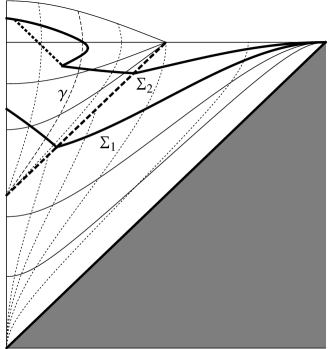
Figure 1: Two constant–CAH time hypersurfaces, $\Sigma_{1}$ and $\Sigma_{2}$ (thick, solid curves), intersecting and extending into a bubble universe. The thin, solid curves correspond to constant-$t$ (constant-$\tau)$ surfaces, while the thin, dotted curves correspond to constant-$r$ (constant-$\xi$) surfaces, in the parent vacuum (bubble). The thick, dashed line approximates the bubble wall, while the thick, dotted line represents the cutoff imposed by the CAH+ measure prescription. A comoving FRW geodesic $\gamma$ is indicated by the dashed line. (See main text.)

Consider for example the FRW geodesic labeled $\gamma$ in Figure 1. This geodesic reaches the cutoff value $\theta_{\rm cut}$ on the surface $\Sigma_{2}$ while it is still in the inflating region. Beyond this point, $\theta$ continues to grow until the end of inflation. Then it decreases until the value $\theta_{\rm cut}$ is reached again. This is where the geodesic crosses $\Sigma_{2}$ for the second time. After this crossing, $\theta$ keeps decreasing until the onset of $\Lambda$ domination, where it starts to grow again, and finally reaches $\theta_{\rm cut}$ for the third time, at the third crossing of $\Sigma_{2}$. If the cosmological constant had been precisely zero, the CAH time $\theta$ would never have resumed increasing with FRW time, and $\Sigma_{2}$ would continue to run to larger values of $\xi$ as $\tau$ is increased, until reaching spacelike infinity. The geodesic $\gamma$ would then cross $\Sigma_{2}$ only twice, while FRW geodesics at sufficiently small values of $\xi$ would never cross $\Sigma_{2}$. The same qualitative picture applies for negative $\Lambda$.

Now, the CAH+ prescription requires that we remove all points in the future light cone of any point on the constant-CAH surface $\Sigma$. This leaves $\Sigma_{1}$ unchanged, but it does modify $\Sigma_{2}$, replacing a part of it with a null hypersurface, as indicated by the thick, dotted line in Figure 1.

So far we have discussed the constant CAH-time foliation in a CDL bubble, which is defined with respect to a spatially flat initial hypersurface $\Sigma_{0}$ in the parent vacuum. One might worry about the generality of this setup. However, during exponential expansion, timelike geodesics rapidly converge to comoving worldlines in the spatially-flat foliation. Furthermore, at late times in a positive vacuum-energy bubble, the CAH-time foliation asymptotes to that of a spatially-flat de Sitter chart (see Appendix A). This means it is not important for the hypersurface $\Sigma_{0}$ to be flat or to have been drawn in the parent vacuum, as opposed to in any previous ancestor vacuum. Any spacelike hypersurface $\Sigma_{0}$ would do, as long as it is placed sufficiently deep in the past of the bubble nucleation event.

2.4 Prior distribution

The bubble nucleation time $\theta_{\rm n}$, although a constant with respect to the evolution of $\theta(\tau,\,\xi)$ in any given bubble, does depend on the history of the subset of the congruence entering the bubble. The statistical properties of $\theta_{\rm n}$ are determined by the coarse-grain rate equation, which tracks the three-volume ${\cal V}_{i}$ occupied by a given vacuum $i$ on surfaces of constant CAH time $\theta$, averaging over (proper) timescales that are large compared to the relevant Hubble times, but small compared to the the relevant inverse decay rates.

It is convenient to start with the rate equation in terms of scale-factor time $t$ [13, 1],

$$\frac{d{\cal V}_{i}(t)}{dt}=3{\cal V}_{i}(t)+\sum_{j}\kappa_{ij}{\cal V}_{j}(t)-\sum_{j}\kappa_{ji}{\cal V}_{i}(t)\,,$$ (10)

where $\kappa_{ij}\equiv(4\pi/3)H_{j}^{-4}\Gamma_{ij}$ is the dimensionless decay rate. This equation is understood to apply only to de Sitter vacua $i$, and the first term on the right-hand-side accounts for the volume expansion during positive vacuum energy domination. The second the second term sums over bubble nucleations of vacuum $i$ in other vacua $j$, and the last term sums over decays of vacuum $i$ to vacua $j$. The last sum is understood to run over de Sitter and Anti–de Sitter (and Minkowski) vacua (the first sum can also be taken to run over all vacua, however only de Sitter vacua contribute since the other transition rates are zero).

To convert to CAH time, first note that the difference between two scale-factor times evaluated at two points “1” and “2” along a given geodesic can be written

$$t_{2}-t_{1}=\ln(a_{2}/a_{1})=\ln(\theta_{2}/\theta_{1})-\ln(H_{2}/H_{1})\,,$$ (11)

where we have used $t=H\tau=\ln(a)=\ln(\theta/H)$ in the spatially-flat slicing of de Sitter space, and the subscripts denote at which point a given quantity is evaluated. It can be shown that this relationship between scale-factor and CAH times holds not only within a single bubble (where $H_{2}=H_{1}$), but also along a geodesic traversing two or more bubbles, so long as the proper time between points “1” and “2” is much larger than the Hubble time.

We have made the scale-factor time dependence of (10) explicit to make clear that converting to CAH time involves not only changing the differential time element,

$$dt\,\to\,d\ln(\theta/\theta_{0})\,,$$ (12)

with $\theta_{0}$ here being an arbitrary scale, but also changing the volume ${\cal V}_{j}(t)$, since surfaces of constant scale-factor time are not surfaces of constant CAH time, in the presence of bubble nucleations. In particular, the volume expansion factor in terms of scale-factor time is $e^{3t}$, and therefore the logarithmic offset of (11) corresponds to a shift in time with concomitant volume expansion factor $(H_{1}/H_{2})^{3}\to(H_{j}/H_{i})^{3}$ multiplying ${\cal V}_{j}$. Thus,

$$\frac{d{\cal V}_{i}(\theta)}{d\ln(\theta/\theta_{0})}=3{\cal V}_{i}(\theta)+\sum_{j}\kappa_{ij}\,(H_{j}/H_{i})^{3}\,{\cal V}_{j}(\theta)-\sum_{j}\kappa_{ji}{\cal V}_{i}(\theta)\,.$$ (13)

Note that this is also the rate equation for the lightcone time measure of [8, 9], since lightcone time and CAH time are equivalent within de Sitter vacua.

It is convenient to define the quantity

$$f_{i}\equiv H_{i}^{3}{\cal V}_{i}\,,$$ (14)

so that the rate equation can be written

$$\frac{df_{i}}{d\ln(\theta/\theta_{0})}=3f_{i}+\sum_{j}\kappa_{ij}f_{j}-\sum_{j}\kappa_{ji}f_{i}\,.$$ (15)

The equation is now a simple change in variables from that studied in [13, 1]. In particular, at late times the solution can be written

$$f_{i}(\theta)=s_{i}\,(\theta/\theta_{0})^{3-q}+\ldots\,,$$ (16)

where $q>0$ is the smallest-magnitude eigenvalue of the transition matrix $\kappa_{ij}-\delta_{ij}\sum_{k}\kappa_{ki}$, $s_{i}$ is the corresponding eigenvector, and the ellipses denote terms that fall off faster than $\theta^{-q}$. Using (14) to solve for ${\cal V}_{i}$, we find

$${\cal V}_{i}(\theta)\propto s_{i}\,(\theta_{0}/H_{i})^{q}\,(\theta/H_{i})^{3-q}\,,$$ (17)

Therefore, the number of bubble nucleations of type $i$ in a CAH time interval $d\theta$ is

$$d{\cal N}_{i}(\theta)=\sum_{j}\Gamma_{ij}\,{\cal V}_{j}(\theta)\,\frac{d\tau}{d\theta}\bigg{|}_{j}d\theta\,\propto\,\sum_{j}\kappa_{ij}s_{j}\,\theta^{2-q}\,d\theta\,.$$ (18)

(The factor $d\tau/d\theta$ in the first expression arises because the rate $\Gamma_{ij}$ is given per unit proper time in the vacuum $j$.) In practice, the exponent $q$ is on the order of the smallest (dimensionless) decay rate among positive-energy vacua in the landscape, and is therefore negligible next to the power of two. The factor

$$P_{i}\propto\sum_{j}\kappa_{ij}s_{j}$$ (19)

gives the relative number of bubbles of type $i$ below the cutoff. It can be regarded as the “prior” probability for this type of bubble.

3 Phenomenology

Section 2.2 describes evolution of CAH time $\theta$ as a function of the coordinates $(\tau,\,\xi)$ in a CDL bubble. To make predictions, we set a cutoff value $\theta_{\rm cut}$, and compute statistics according to the relative numbers of different types of events between the initial hypersurface $\Sigma_{0}$ and the cutoff hypersurface $\Sigma_{\rm cut}$. We focus on the subset of bubbles that are indistinguishable from ours, except for the value of the cosmological constant $\Lambda$ and the number of inflationary $e$-folds $N$. The events of interest to us here are the observations of $\Lambda$ and $N$, so they can be labeled by the same index $i$ as the bubbles. The number of such events in bubbles of type $i$ between $\Sigma_{0}$ and $\Sigma_{\rm cut}$ can be written as

$${\cal N}_{i}\propto P_{i}\int_{\theta_{0}}^{\theta_{\rm cut}}d\theta_{\rm n}\,\theta_{\rm n}^{2-q}\int_{0}^{\tau_{\rm cut}}d\tau\,\overline{a}^{3}(\tau)\,\rho_{i}(\tau)\int_{0}^{\xi_{\rm cut}}d\xi\,\sinh^{2}(\xi)\,.$$ (20)

Here $P_{i}$ is the prior probability (19) for bubbles of type $i$, $\rho_{i}(\tau)$ is the number of relevant observations per unit physical four-volume in such bubbles, $\xi_{\rm cut}(\tau,\,\theta_{\rm n},\,\theta_{\rm cut})$ is the value of $\xi$ at which the constant-$\tau$ hypersurface intersects the cutoff hypersurface, and $\tau_{\rm cut}(\theta_{\rm n},\,\theta_{\rm cut})$ is the maximum FRW proper time in the bubble probed by the cutoff hypersurface. Moving from right to left, the first two integrations count the number of observations under the cutoff in a bubble of type $i$ nucleating at CAH time $\theta_{\rm n}$, while the last integral sums over bubble nucleation times, according to Eq.(18). Since $q$ is exponentially small, we henceforth drop it.

Since the CAH+ measure prescription involves augmenting the cutoff hypersurface with lightcones, it is convenient to work in terms of the bubble conformal time $\eta=\int d\tau/\overline{a}(\tau)$, as opposed to the proper time $\tau$. During the early-time inflationary epoch in the bubble, i.e. for $|\eta_{\star}|\ll|\eta|\ll 1$, where $\eta_{\star}=-2e^{-N}$ is the reheating time, CAH time is given by

$$\theta(\eta,\,\xi)=-\frac{\theta_{\rm n}}{\eta}\,e^{\xi}\,.$$ (21)

After inflation, (21) no longer holds. (We assume instantaneous reheating.) As described in Section 2.2, during radiation, non-relativistic matter, and spatial-curvature domination, $\theta$ decreases along comoving geodesics. The would-be cutoff hypersurface $\theta=\theta_{\rm cut}$ therefore runs toward increasing $\xi$ with increasing $\eta$, and in the CAH+ prescription it is augmented by the future lightcone of where it intersects the reheating hypersurface, $\theta=(1/2)\,\theta_{\rm n}\,e^{\xi+N}$. When $\eta>\eta_{\star}$, this lightcone provides the cutoff

$$\xi_{\rm cut}=-\eta+\eta_{\star}+\ln(2\theta_{\rm cut}/\theta_{\rm n})-N\,.$$ (22)

The events that concern us (observers like us measuring cosmological parameters) occur only after non-relativistic matter domination, when $\eta\gg\eta_{\star}$, so henceforth we drop $\eta_{\star}$ next to $\eta$.

In bubbles with zero or negative cosmological constant, the cutoff (22) applies to all times after reheating. In bubbles with positive cosmological constant, however, $\theta$ begins to increase again at cosmological-constant domination, and the $\theta=\theta_{\rm cut}$ hypersurface can supercede (22). The evolution of $\theta$ after cosmological-constant domination is determined by (7), substituting conformal time $\eta$ for proper time $\tau$ (see Appendix B). The result depends on whether or not there is a period of spatial-curvature domination after non-relativistic matter domination, in particular:

$$\theta=\left\{\,\,\begin{array}[]{ll}\displaystyle\frac{\theta_{\rm n}\,e^{\xi}}{3-\ln(\textstyle\frac{3}{2}H_{\Lambda}\tau_{\rm c})-\eta}\quad\!\!&\phantom{\Bigg{[}\Bigg{]}}\mbox{if there is curvature domination}\\ \displaystyle\frac{\theta_{\rm n}\,e^{\xi}}{(\textstyle\frac{1}{18}H_{\Lambda}\tau_{\rm c})^{-1/3}-\eta}\quad\!\!&\phantom{\Bigg{[}\Bigg{]}}\mbox{if not}\,,\end{array}\right.$$ (25)

where $H_{\Lambda}\equiv\sqrt{|\Lambda|/3}$, and $\tau_{\rm c}$ is the time at which spatial curvature would begin to dominate, if $H_{\Lambda}$ were zero. In each case the expression is valid after the onset of cosmological-constant domination at $\eta_{\Lambda}$, corresponding to when the denominator is equal to unity.

When (positive) cosmological-constant domination follows a period of spatial-curvature domination, the hypersurface $\theta=\theta_{\rm cut}$ is obtained by inverting the upper of (25), and gives

$$\xi_{\rm cut}=\ln\!\left[3-\ln\!\left(\textstyle\frac{3}{2}H_{\Lambda}\tau_{\rm c}\right)-\eta\right]+\ln(\theta_{\rm cut}/\theta_{\rm n})\,.$$ (26)

This is the actual CAH+ cutoff when it provides a stronger constraint than the future lightcone cutoff (22), so the cutoff is given by the smaller of (22) and (26). Since both of these expressions are monotonically decreasing, (22) provides the cutoff up to some time $\eta_{1}$, after which (26) provides the cutoff, with $\eta_{1}$ corresponding to the solution of

$$2e^{-\eta_{1}-N}=3-\ln\!\left(\textstyle\frac{3}{2}H_{\Lambda}\tau_{\rm c}\right)-\eta_{1}\,.$$ (27)

A similar story holds when non-relativistic matter domination gives way directly to (positive) cosmological-constant domination. In this case the $\theta=\theta_{\rm cut}$ hypersurface gives

$$\xi_{\rm cut}=\ln\!\left[\left(\textstyle\frac{1}{18}H_{\Lambda}\tau_{\rm c}\right)^{-1/3}-\eta\right]+\ln(\theta_{\rm cut}/\theta_{\rm n})\,.$$ (28)

As before, the actual CAH+ cutoff is given simply by the smaller of (22) and (28). Likewise, (22) provides the cutoff up to some time $\eta_{2}$, after which (28) provides the cutoff, with $\eta_{2}$ corresponding to the solution of

$$2e^{-\eta_{2}-N}=\left(\textstyle\frac{1}{18}H_{\Lambda}\tau_{\rm c}\right)^{-1/3}-\eta_{2}\,.$$ (29)

Henceforth we refer to the above transition times as $\eta_{1,2}$, with it being understood that $\eta_{1}$ applies to when non-relativistic matter domination gives way directly to cosmological constant domination (which corresponds to $\tau_{\rm c}\geq(2/3)H_{\Lambda}^{-1}$), and $\eta_{2}$ applies when there is a period of late-time spatial-curvature domination (corresponding to $\tau_{\rm c}<(2/3)H_{\Lambda}^{-1}$).

Putting the above results together, it is convenient to write

$$\xi_{\rm cut}(\eta,\theta_{\rm n})=-f(\eta)+\ln(\theta_{\rm cut}/\theta_{\rm n})\,,$$ (30)

with $f(\eta)$ given by

$$f(\eta)=\left\{\,\,\begin{array}[]{ll}\displaystyle\eta+N-\ln(2)\phantom{\bigg{[}\bigg{]}}&\parbox{205.0pt}{ if $\Lambda\leq 0$, or \\ if $\Lambda>0$ and $\eta<\eta_{1,2}$}\\ \displaystyle\ln\!\big{[}H_{\Lambda}\overline{a}(\eta)\big{]}\phantom{\bigg{[}\bigg{]}}&\parbox{200.0pt}{ if $\Lambda>0$ and $\eta\geq\eta_{1,2}$\,,}\\ \end{array}\right.$$ (33)

where we have used the results of Appendix B to recognize the dependence on $\overline{a}$. We are now prepared to return to (20). Performing the integration over $\xi$, we obtain

$${\cal N}_{i}\propto P_{i}\int_{\theta_{0}}^{\theta_{\rm cut}}d\theta_{\rm n}\,\theta_{\rm n}^{2}\int_{\eta_{\star}}^{f^{-1}[\ln(\theta_{\rm cut}/\theta_{\rm n})]}\!d\eta\,\,\overline{a}^{4}(\eta)\,\rho_{i}(\eta)\,\Big{\{}\sinh\!\big{[}2\xi_{\rm cut}(\eta,\theta_{\rm n})\big{]}-2\xi_{\rm cut}(\eta,\theta_{\rm n})\Big{\}}\,.\,\,$$ (34)

It is possible to exchange the order of $\theta_{\rm n}$ and $\eta$ integration. It is also worthwhile to change the integration variable $\theta_{\rm n}$ to $y\equiv\ln(\theta_{\rm cut}/\theta_{\rm n})-f(\eta)$. These operations allow us to write

$${\cal N}_{i}\propto P_{i}\int_{\eta_{\star}}^{\eta_{\rm max}}\!d\eta\,\,\overline{a}^{4}(\eta)\,\rho_{i}(\eta)\,e^{-3f(\eta)}\,{\cal I}(\eta)\,,$$ (35)

where $\eta_{\rm max}\equiv\min\{\,\ln(\theta_{\rm cut}/\theta_{0}),\mbox{the maximum value of $\eta$ reached in the bubble}\}$, and

$${\cal I}(\eta)\equiv\int_{0}^{\ln(\theta_{\rm cut}/\theta_{0})-f(\eta)}dy\,e^{-3y}\Big{[}\sinh(2y)-2y\Big{]}\,.$$ (36)

In the limit $\theta_{\rm cut}\to\infty$, assuming that $\rho_{i}(\eta)$ is localized within some finite range of $\eta$, we can take the upper limit of integration of ${\cal I}(\eta)$ to infinity, so that ${\cal I}(\eta)$ becomes a constant.

3.1 Geometric effects

Before focusing on the implications of (35) for observers like us, it is worthwhile to investigate some of the more general features of this result. Toward this end we here adopt a more crude “anthropic” model, which places all observers at some fixed FRW proper time $\tau_{\rm obs}$ in the bubble, and takes the density of their observations to be proportional to the density of non-relativistic matter. (Our analysis follows the spirit of [2].) Intuitively, it would be preferable to place the observers at some fixed proper time after reheating, but we assume $\tau_{\rm obs}\gg NH_{\rm d}^{-1}$ so that the difference is negligible. To be precise, we write

$$\rho_{\rm obs}(\eta)\propto\frac{\overline{a}^{3}(\eta_{\star})}{\overline{a}^{4}(\eta)}\,\delta\big{[}\eta-\eta(\tau_{\rm obs})\big{]}\,,$$ (37)

where $\delta$ is the Dirac delta function, and we have included a factor of $|d\tau/d\eta|^{-1}=\overline{a}^{-1}$ to account for the measure of integration, as well as a factor of $\overline{a}^{3}(\eta_{\star})$ because inflationary expansion does not dilute the density of non-relativistic matter after reheating. This gives

$${\cal N}_{\rm obs}\propto P(\Lambda,N)\,e^{3N-3f[\eta(\tau_{\rm obs})]}\,,$$ (38)

where the “prior” $P(\Lambda,N)$ is the probability that a random bubble will be characterized by given values of $N$ and $\Lambda$ and be otherwise identical to ours.

It is convenient to express $\Lambda$ and $\tau_{\rm c}(N)$ in units of $\tau_{\rm obs}$. Accordingly, we write

$$\ell={\rm sign}(\Lambda)\,(H_{\Lambda}\tau_{\rm obs})^{2}\,,\qquad{\rm and}\qquad\tau_{\rm c}=\tau_{\rm obs}\,e^{3(N-N_{\rm obs})}\,,$$ (39)

where $N_{\rm obs}$ depends on the details of the cosmological history. Then $\ell\approx 1$ corresponds to observers arising at about the onset of cosmological-constant domination, and $N=N_{\rm obs}$ corresponds to observers arising at the onset of spatial-curvature domination (in bubbles where this happens). If we consider $\ell$ and $\tau_{\rm c}$ to be fixed and study ${\cal N}_{\rm obs}$ as a distribution over $\tau_{\rm obs}$, then we find the distribution features two qualitatively distinct regimes. For positive $\ell$ and sufficiently large $\tau_{\rm obs}$, we have $\eta(\tau_{\rm obs})\geq\eta_{1,2}$ and ${\cal N}_{\rm obs}\propto e^{3N}\big{[}H_{\Lambda}\overline{a}(\tau_{\rm obs})\big{]}^{-3}$. Thus ${\cal N}_{\rm obs}$ is proportional to the density of non-relativistic matter. For smaller $\tau_{\rm obs}$, as well as for $\ell\leq 0$, ${\cal N}_{\rm obs}\propto e^{-3\eta(\tau_{\rm obs})}$. This corresponds to a weaker (decreasing) function of $\tau_{\rm obs}$ than the density of non-relativistic matter. Thus we conclude that ${\cal N}_{\rm obs}$ prefers smaller values of $\tau_{\rm obs}$, but the effect is not stronger than the youngness bias of the scale-factor cutoff or fat geodesic measures [15, 16]. In particular, if we were to condition on structure formation, ${\cal N}_{\rm obs}$ would become strongly suppressed for sufficiently small $\tau_{\rm obs}$, resulting in a localized distribution. To simplify the discussion, for the rest of this subsection we assume $\tau_{\rm obs}$ is fixed, and corresponds to some time during or after non-relativistic matter domination.

Since the CAH+ measure does not exponentially favor large amounts of inflation in the bubble, it does not suffer from the $Q$ and $G$ catastrophes [17, 18, 19]. Note that the CAH+ measure can also avoid Boltzmann-brain domination [20, 21, 22]. In particular, we found above that for sufficiently late times, $\eta(\tau_{\rm obs})\geq\eta_{1,2}$, the measure samples in proportion to $a(\tau_{\rm obs})^{-3}$. Modulo proportionality constants, this is the same late-time behavior as the causal patch, scale-factor cutoff, and fat geodesic measures, each of which has been shown to be able to avoid Boltzmann-brain domination [23, 1, 16]. As is discussed in those papers, the early-time behavior is unimportant compared to the huge timescales on which Boltzmann brains typically form. Similarly the differing proportionality constants are inconsequential next to Boltzmann-brain nucleation rates and vacuum decay rates that dominate the calculations.

Consider now ${\cal N}_{\rm obs}$ as a distribution over $N$, keeping $\ell$ (and $\tau_{\rm obs}$) fixed. For $N<N_{\rm obs}$ and $|\ell|<2/3$, the time $\tau_{\rm obs}$ corresponds to during spatial-curvature domination. In this regime, $\eta(\tau_{\rm obs})<\eta_{1,2}$, so we have ${\cal N}_{\rm obs}\propto e^{-3\eta(\tau_{\rm obs})}$. Using (81), we find ${\cal N}_{\rm obs}\propto\big{(}\frac{2}{3}e^{3(N_{\rm obs}-N)}+\frac{1}{3}\big{)}^{-3}$, i.e. the distribution is exponentially suppressed for $N$ significantly less than $N_{\rm obs}$. Surveying increasing values of $N$, $\tau_{\rm obs}$ corresponds to during non-relativistic matter domination and ${\cal N}_{\rm obs}/P$ asymptotes to a constant. The transition from exponentially increasing in $N$ to independent of $N$ occurs rather sharply at $N\sim N_{\rm obs}$; thus, for prior distributions $P$ that are (negative) power laws in $N$, the distribution ${\cal N}_{\rm obs}$ is peaked at $N\sim N_{\rm obs}$, but can have a long tail toward large $N$. The above discussion applies only to $|\ell|<2/3$, yet for larger values of $|\ell|$ the story is mostly the same: for a given value of $N$ the time $\tau_{\rm obs}$ may correspond to during cosmological-constant domination instead of during spatial-curvature or non-relativistic matter domination, but overall the dependence of ${\cal N}_{\rm obs}/P$ on $N$ is qualitatively unchanged from above. The only significant development occurs when $\ell$ becomes so large that $\eta(\tau_{\rm obs})>\eta_{1,2}$, in which case ${\cal N}_{\rm obs}/P$ becomes strictly independent of $N$. As indicated in the next paragraph, ${\cal N}_{\rm obs}/P$ is suppressed in this region of the parameter space.

Finally, we discuss the dependence of ${\cal N}_{\rm obs}$ on $\ell$, keeping $N$ and $\tau_{\rm obs}$ fixed. Starting at sufficiently small values of $|\ell|$, the time $\tau_{\rm obs}$ corresponds to during non-relativistic matter or spatial-curvature domination, and ${\cal N}_{\rm obs}/P$ is independent of $\ell$. Surveying increasing values of $|\ell|$, eventually $\tau_{\rm obs}$ corresponds to during cosmological-constant domination. When $\ell<0$, ${\cal N}_{\rm obs}/P$ is a weakly decreasing function of $|\ell|$, until the minimum-allowed value of $\ell$ is reached when $\tau_{\rm obs}$ coincides with the big-crunch singularity at $\ell\sim-(2\pi/3)^{2}$, the precise value of the bound depending weakly on $N$. When $\ell>0$ the distribution ${\cal N}_{\rm obs}/P$ is a weakly increasing function of $\ell$, until $\eta(\tau_{\rm obs})$ becomes greater than $\eta_{1,2}$, after which the distribution decreases exponentially in $\ell$. It can be shown that this transition occurs roughly at $\ell^{1/2}+\ln(\ell^{1/2})\sim 3N_{\rm obs}-2N$, when $Ne^{3(N-N_{\rm obs})}\lesssim 1$, or at $\ell^{1/2}+(1/3)\ln(\ell^{1/2})\sim N_{\rm obs}$, when $Ne^{3(N-N_{\rm obs})}\gtrsim 1$. If we neglect the logarithms and use $N\sim N_{\rm obs}$ from the previous paragraph, we see that the scale of $\ell$ is set by $N_{\rm obs}^{2}$. In bubbles otherwise like ours, $N_{\rm obs}$ can be as large as $60$ (for GUT-scale inflation), setting the scale at a few thousand times the value of the cosmological constant we observe. As we shall see, however, further consideration of anthropic selection effects for observers like us can suppress such large values of $\ell$.

Figure 2: Contour plot of the distribution ${\cal N}_{\rm obs}/P$ in the $(N,\ell)$ plane (the distribution peaks toward the right and center). We have set $N_{\rm obs}=5$ to condense the scale of the plot.

These results are illustrated in Figure 2. We have chosen $N_{\rm obs}=5$ so as to reduce the range of coordinates. As a function of increasing $N$ (with $\ell\lesssim N_{\rm obs}^{2}$) the distribution rises smoothly from at about $N_{\rm obs}$, and flattens out several $e$-folds beyond that. (If we were to include a prior of the form $P(N)\propto N^{-\alpha}$, $\alpha>1$, the distribution would be peaked at several $e$-folds above $N_{\rm obs}$.) As a function of decreasing $\ell$, the distribution rises sharply at $\ell\sim N_{\rm obs}^{2}$, and then decreases slowly until the minimum-allowed value of $\ell$ is reached. Note that, unlike the causal patch, apparent horizon cutoff, and fat geodesic measures studied in [2], the CAH+ measure is free of divergences in the $(\ell,N)$ plane.

3.2 Anthropic selection

We are interested in the distributions of values of $\Lambda$ and $N$ measured by observers like us. The restriction to observers like us is important because we wish to test these distributions against the value of $\Lambda$ and lower bound on $N$ that we actually observe, and such comparisons are meaningful only insofar as we can assert that the values we observe should be considered as randomly drawn from the predicted distributions. Insofar as our presence to measure these quantities correlates with their physical values, these correlations must be taken into account.

What is meant by the qualification “like us” defines the precise hypothesis that is being tested, and is ultimately constrained by our understanding and acumen. According to the “principle of mediocrity” [24, 25], we should consider ourselves typical in (that is, randomly drawn from) any class of observers to which we belong, unless we have evidence to the contrary. In the latter case, the class should be correspondingly narrowed. As more data is accumulated and our models are improved, we will be able to specify a narrower reference class of observers and make more accurate predictions.

Here we simply assume that the density of observers like us at a given FRW proper time $\tau$ is proportional to the number of galaxies that passed a certain mass threshold $M$ a certain proper time $\Delta\tau$ before $\tau$. (We do not distinguish between non-relativistic baryons and cold dark matter, and by “galaxy” we refer to both the visible structure and the halo.) The basic idea is that a galaxy should have a certain minimum mass, to permit efficient star formation and likewise to have produced and retained heavy elements, and should have existed for a certain time, to permit planetary and biological evolution. With respect to bubbles with negative cosmological constant, we pursue two possibilities:

• in this case we do not include FRW times after $\tau_{\rm turn}$, the time of scale-factor turnaround, presuming that the typically-high merger rate in such circumstances is hazardous to stable stellar systems in which observers like us can arise,

• in this case we include all times, ignoring the above effect.

To be concrete, we take $M=10^{12}$ solar masses and $\Delta\tau=5$ Gyr. (These anthropic assumptions are the same as those adopted and further explained in [15].)

To determine the rate at which galaxies exceed the mass $M$, we work in the Press-Schechter formalism [26]. The main result of this approach is the collapse fraction (of non-relativistic matter) into galaxies of mass greater than or equal to $M$ by proper time $\tau$,

$$F_{\rm c}(M,\,\tau)={\rm erfc}\!\left[\frac{\delta_{\rm c}(\tau)}{\sqrt{2}\,\sigma_{\rm rms}(M,\tau)}\right],$$ (40)

where erfc denotes the complimentary error function, $\sigma_{\rm rms}(M,\tau)$ is the amplitude of a root-mean-square (rms) density perturbation on a comoving scale enclosing a mass $M$ (according to the linearized equation of motion), and $\delta_{\rm c}(\tau)$ corresponds to the amplitude that a density perturbation must have reached, according to the linearized equation of motion, for it to correspond to a collapsed spherical top-hat over-density at time $\tau$ (the spherical top hat being evolved according to a non-linear analysis). The collapse threshold $\delta_{\rm c}$ is in general a function of time, however for our purposes it is sufficient to use the late-time asymptotic values $\delta_{\rm c}=1.72$ for $\Lambda<0$, $\delta_{\rm c}=1.50$ for $\Lambda=0$, and $\delta_{\rm c}=1.63$ for $\Lambda>0$. (At least in the case where there is no period of late-time spatial-curvature domination, this approximation was found to be accurate at the percent level by the authors of [15]).

The rate at which galaxies exceed the mass $M$ is simply the time derivative of $F_{\rm c}$. Incorporating the time delay mentioned above, we have for the density of observers

$$\rho_{\rm obs}(\tau)\propto\frac{\overline{a}^{3}(\tau_{\star})}{\overline{a}^{3}(\tau)}\frac{dF_{\rm c}}{d\tau}\bigg{|}_{M,\,\tau-\Delta\tau}\,,$$ (41)

where it is understood that $\rho_{\rm obs}=0$ for $\tau>\tau_{\rm turn}$ when considering case ($i$) above. Inserting into (35), we obtain

$${\cal N}_{\rm obs}(\Lambda,\,N)\propto P(\Lambda,\,N)\int_{\Delta\tau}^{\tau_{\rm max}}d\tau\,e^{3N-3f[\eta(\tau)]}\,\frac{dF_{\rm c}}{d\tau}\bigg{|}_{M,\,\tau-\Delta\tau}\,,$$ (42)

where for $\Lambda<0$, we use $\tau_{\rm max}=\tau_{\rm turn}$ for case ($i$) and $\tau_{\rm max}=\tau_{\rm crunch}=2\tau_{\rm turn}$ for case ($ii$), while for $\Lambda\geq 0$, we use $\tau_{\rm max}\to\infty$.

Since anthropic selection will strongly suppress all values of $\Lambda$ except those within a very small (compared to the Planck or electroweak scales) window about zero, the prior distribution of $\Lambda$ is expected to be flat [27]. (The conditions of validity of this heuristic argument have been studied in several simple landscape models [28, 29, 30], with the conclusion that it does in fact apply to a wide variety of scenarios.) We shall assume that the argument is valid, so the prior probability is independent of $\Lambda$. The appropriate prior distribution for the number of $e$-folds $N$ is less clear; here we simply lift the distribution obtained by [31], based on randomly scanning the parameters of a linearized scalar-field potential. Together these give the distribution

$$P(\Lambda,\,N)\propto N^{-4}\,.$$ (43)

The distribution ${\cal N}_{\rm obs}$ can be evaluated numerically, given $\overline{a}(\tau)$, $\eta(\tau)$, and $\sigma_{\rm rms}(M,\,\tau)$. Each of these quantities is approximated in Appendix B, and during the relevant times can be expressed entirely in terms of $H_{\Lambda}$, $\tau_{\rm c}$, and the density contrast $\sigma_{\rm ref}(M)$ evaluated at some reference time $\tau_{\rm ref}$. It is convenient to write

$$\lambda={\rm sign}(\Lambda)\,(H_{\Lambda}/\tilde{H}_{\Lambda})^{2}\,,\qquad{\rm and}\qquad\tau_{\rm c}=\tilde{H}_{\Lambda}^{-1}e^{3(N-N_{\Lambda})}\,,$$ (44)

where $\tilde{H}_{\Lambda}$ is the value of $H_{\Lambda}$ measured in our universe, $\tilde{H}_{\Lambda}^{-1}=16.3$ Gyr, and

$$N_{\Lambda}=\frac{1}{3}\ln\!\left(3\cdot 2^{5/2}H_{\rm d}^{3/2}\tau_{\rm eq}^{1/2}\tilde{H}_{\Lambda}^{-1}\right).$$ (45)

Since $N_{\Lambda}$ depends on $H_{\rm d}$, its precise value in our universe is not known (in our simple model of inflation and reheating $H_{\rm d}\approx 10^{3}\mbox{--}10^{15}$ GeV would correspond to $N_{\Lambda}\approx 50\mbox{--}64$). Nevertheless, after the onset of non-relativistic matter domination the evolution of the universe depends only on the difference $N-N_{\Lambda}$, and so dependence on $N_{\Lambda}$ by itself enters only via the relative effect of the prior distribution $P(\Lambda,\,N)$, and this effect is approximately independent of $N_{\Lambda}$ when $N_{\Lambda}\gg 1$. For concreteness we choose $N_{\Lambda}=60$. Finally, we note that the data of footnote 4 correspond to setting $\sigma_{\rm ref}(M)$ so that deep into the epoch of non-relativistic matter domination, we have $\sigma_{\rm rms}(M=10^{12}M_{\odot})=2.50\,(\tilde{H}_{\Lambda}\tau)^{2/3}$.

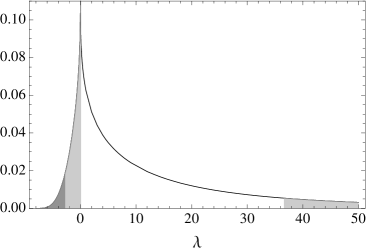
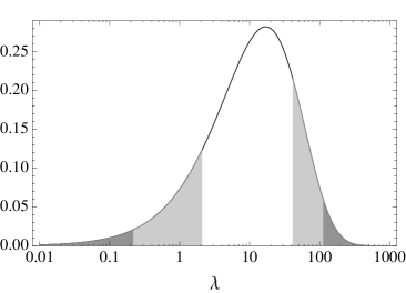
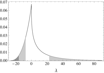
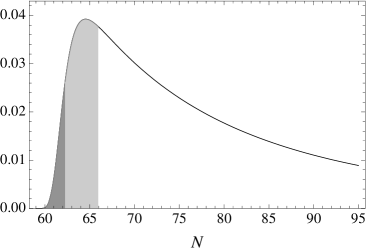
Figure 3: Slices of the (normalized) distribution ${\cal N}_{\rm obs}(\lambda,\,N)$. The left panels display the distribution over all $\lambda$, for anthropic case ($i$) (top) and case ($ii$) (bottom), for $N=70$. The right panels display the distribution over positive $\lambda$ (top), again using $N=70$, and the distribution over $N$ (bottom), for $\lambda=1$. In each case we use $N_{\Lambda}=60$. Observation gives $\lambda=1$ and $N\geq 62.1$. Regions more than one and two standard deviations away from the median indicated by shading.

In Figure 3 we plot slices of the distribution ${\cal N}_{\rm obs}(\lambda,N)$. Recall that the parameter $\lambda$ has been defined so that our universe corresponds to $\lambda=1$. Meanwhile, the observational constraint on the curvature parameter $\Omega_{k}=(\overline{a}H)^{-2}$ implies a constraint on $\Delta N$; in particular $\Delta N\geq 2.1$ (95% confidence level lower bound), which for $N_{\Lambda}=60$ corresponds to $N\geq 62.2$. (Here we have combined the data of footnote 4 with the scale-factor approximations of Appendix B, with the present FRW time corresponding to just after the onset of cosmological-constant domination). We see that the distributions provide a good fit to the observed value of $\lambda$, whether we allow for negative $\lambda$ or not (indeed, regardless of whether we impose anthropic condition ($i$) or not), at least when there is much more than sufficient inflation, as in our universe. Note that the sharp peak at $\lambda=0$ is not a divergence. The results are consistent with what is found in Section 3.1, with the distribution being more sharply peaked about $\Lambda=0$ than in that analysis because we have conditioned on the formation of galaxies like ours, which becomes inhibited for large positive values of $\lambda$.

Regarding the distribution of $N$, we see the probability is highly suppressed for $N<N_{\Lambda}$, in accordance with what was found in Section 3.1. As in that analysis, the distribution would rise and asymptote to a constant value as $N$ is increased over the next several $e$-folds; however we have included the prior (43), which selects for smaller values of $N$, hence the peaked distribution of Figure 3. Given the location of the peak and its long, large-$N$ tail, it is evident that the distribution is consistent with the present observational limit, $N\geq 62.2$ for $N_{\Lambda}=60$ (corresponding to $\Omega_{k}\leq 8.3\times 10^{-3}$, see footnote 4). Our ability to detect spatial curvature (for instance, via its effects on the CMB) is cosmic-variance limited [34, 35], and it is worthwhile to ask the following question. Given this model, and given the present observational limit, what is the likelihood that $N$ lies in the range amenable to future detection? To quickly estimate the answer, following [31] we crop the distribution at the present observational bound, and compute the fraction of the remaining distribution for which $\Omega_{k}\leq 10^{-4}$ ($N\geq 64.3$), finding that it is 0.077. Thus, there is reasonable hope for a future detection. These results are similar to those found in [33] for the distribution of $N$ in the scale-factor cutoff measure, and the discussion there concerning other possibilities for the prior distribution $P(N)$ applies here as well.

In Figure 4 we provide a contour plot of ${\cal N}_{\rm obs}(\lambda,N)$, in the $(N,\lambda)$ plane, for case ($i$). Although it might appear as if constant-$N$ slices might represent different distributions of $\lambda$ as one surveys increasing $N$, in fact (for $N$ significantly larger than $N_{\Lambda}$) all that changes is the overall normalization, according to the $N$-dependence of the prior (43).

Figure 4: Contour plot of the distribution ${\cal N}_{\rm obs}(\lambda,N)$, for case ($i$), assuming $N_{\Lambda}=60$.

4 Summary of measure proposals

To provide context for the results of Section 3, we briefly summarize the major qualitative, phenomenological characteristics of several measure proposals. In many cases we simply restate the conclusions of [2] (however we draw different conclusions about the scale-factor cutoff measure), and, as in that analysis, we focus on the predictions for the cosmological constant $\ell$ and the number of $e$-folds $N$ relative to $N_{\rm obs}$ (we use the notation of Section 3.1). We restrict attention to a subset of measures that have been demonstrated to avoid the youngness paradox [36, 37, 38], the Boltzmann brain problem [20, 21, 22] (at least for landscapes with sufficiently rapid decay rates), and the $Q$ and $G$ catastrophes [17, 18, 19].

The geometric cutoff measures that have been discussed so far can be divided into two broad categories: global and local measures. Global measures introduce a cutoff at a fixed value of some global time variable $t$, be it the proper time [39, 40, 41, 42], scale-factor time [41, 42, 15], lightcone time [16], or CAH time, and find the relative numbers of events in the limit $t\to\infty$. An attractive property of these measures is that the resulting distributions do not depend on the choice of the comoving region that is being sampled, reflecting the attractor behavior of eternal inflation. (They do depend on the choice of the time variable $t$.) Local measures sample a spacetime region in the vicinity of a given worldline. The first proposal of this kind is the causal patch measure [43], which counts events that occur within the causal patch of the wordline. (The causal patch could either be the past lightcone of the future endpoint of the worldline, or the causal diamond of the worldline; the two choices give essentially the same phenomenology). This measure was motivated by the idea of “horizon complementarity” [20, 44], suggesting that semi-classical gravity can be trusted only within a causal patch of spacetime accessible to a single observer. Other local measures include the apparent horizon [2] and fat geodesic [16] measures, which sample respectively the region within the apparent horizon and within a fixed geometric distance of the worldline.

All local measures are sensitive to the choice of the initial vacuum where the geodesic begins, so one needs to consider an ensemble of observers with different initial conditions. Without specifying such an ensemble, these measures remain essentially undefined.

The key to specifying the appropriate ensemble may be provided by the recently-discovered duality [45] between local and global measures: the local measure is equivalent to the global measure if the ensemble of initial vacua for the local measure is given by the attractor distribution of the corresponding global measure. (This global-local duality is somewhat limited. As we discuss below, its validity with respect to the fat geodesic measure and scale factor cutoff measure breaks down in AdS vacua.) Thus, one can define the causal patch, apparent horizon, and fat geodesic measures by requiring that the initial distribution should be taken, respectively, from the global lightcone, CAH, and scale factor cutoff measures. Note however that these measures rely on a global picture of spacetime, so that these definitions seem to undermine the initial motivation for the causal patch measure.

Some alternative proposals for specifying the initial distribution can be found in [46]. This distribution could also be determined by the wave function of the universe [43]. Whatever prescription is chosen, one can expect that the arguments we gave concerning the “prior” distribution of $\Lambda$ and $N$ should apply here as well, allowing to predict distributions for these quantities regardless of the precise nature of the ensemble. In the rest of this section we discuss some qualitative features of the resulting distributions, focusing on the divergent, or ”runaway”, behavior exhibited by some of the measures.

We begin with the (local) apparent horizon cutoff measure. According to Figure 4 of [2], when $\ell$ is positive this measure predicts a distribution ${\cal N}_{\rm obs}$ that is peaked toward $\ell=0$ (with $\ln(\lambda)$ peaked at order unity) and at $N\sim N_{\rm obs}$ (if the prior $P(N)$ features power-law preference for smaller $N$). When $\ell$ is negative, ${\cal N}_{\rm obs}$ features a runaway toward decreasing $|\ell|$ and decreasing $N$. Although the results we are quoting ignore anthropic selection effects, it is hard to see how anthropic selection could mitigate the runaway toward small $|\ell|$. Therefore only the discreteness of (anthropic) landscape cuts off the divergence, so that this measure predicts the overwhelming majority of observers to live in some vacuum with a negative cosmological constant very near to zero, in conflict with our observation.

The causal patch measure exhibits the same qualitative behavior for $\ell<0$ [2]. At the same time, this measure features a runaway toward small $\ell$, when $\ell>0$. The runaway is much weaker for positive $\ell$ (where it increases like $\ell^{-1}$) than for negative $\ell$ (where it increases like $|\ell|^{-2}$). This implies once again that the overwhelming majority of observers live in some negative-$\ell$ vacuum.

The authors of [2] turn the runaway for $\ell>0$ into a prediction: assuming the runaway for $\ell<0$ is somehow resolved (and in a way that does not leave behind the milder, but still discouraging preference for negative $\ell$ found in [47]), we should expect to observe the smallest (positive) value of $\ell$ among the subset of vacua that are not extraordinarily rare in the multiverse, and in which observers are not too strongly suppressed. Then $\Lambda$ is expected to be on the order of one over the number of such vacua in the landscape (in Planck units).

This is an interesting attempt to relate the size of the landscape to the observed value of $\Lambda$. The danger here is that the distribution of $\Lambda$ is expected to be very “jagged” on the smallest energy scales, with one value of $\Lambda$ heavily preferred or heavily disfavored next to a nearest neighbor [28, 29, 30]. If the landscape is sufficiently enormous, one might expect this jaggedness to occur only on scales that are very small compared to any scale of interest, leaving an approximately smooth, flat distribution when averaged over an intermediate scale. If however $\Lambda$ is on the order of one over the number of vacua in the landscape, then this jaggedness will be relevant to the prediction of $\ell$, perhaps giving large preferential weight to values that would otherwise seem hostile to observers. Further investigation of this issue is required to draw more definite conclusions.

The properties of the fat geodesic measure can be read off Figure 5 of [2]. When $\ell$ is positive this measure predicts a distribution ${\cal N}_{\rm obs}$ that is peaked toward $\ell=0$ (with $\ln(\ell)$ peaked at order unity) and $N\sim N_{\rm obs}$ (if the prior $P(N)$ features power-law preference for smaller $N$). When $\ell$ is negative, ${\cal N}_{\rm obs}$ features a runaway toward $\tau_{\rm obs}\to\tau_{\rm crunch}$, where $\tau_{\rm crunch}$ is the FRW proper time of the big crunch singularity in these cosmologies. This runaway stems from the fact that a fixed physical volume encloses a diverging quantity of matter as the scale factor tends toward zero. It is not hard to see how anthropic selection alleviates the problem, since the universe will become hotter and denser as the scale factor contracts, and the environment will at some point become hostile to observers. This formally cuts off the divergence in the distribution as $\tau_{\rm obs}\to\tau_{\rm crunch}$, but to what extent the resulting distribution prefers negative $\ell$ depends on the anthropic criteria that are added to the computation.

It should be noted that the apparent horizon and fat geodesic measures violate the causality condition mentioned in the introduction, which requires that the cutoff surfaces should be spacelike. For the causal patch measure the cutoff surface is null and can be made spacelike by an infinitesimal deformation.

We finally discuss the global scale-factor (SF) cutoff measure. It imposes a cutoff at a fixed value of the SF time, which was defined in [15, 1] as (the logarithm of) the volume expansion factor along the geodesic congruence. As it stands, this definition is not satisfactory, since the resulting measure is sensitive to the details of structure formation in thermalized regions of spacetime [16]. Moreover, the cutoff hypersurface obtained with this measure have timelike segments in the vicinity of gravitationally-collapsed structures and in bubbles with negative vacuum energy after scale-factor turnaround. This can be dealt with by augmenting the cutoff hypersurface with the future lightcones of all points on the cutoff, as with the “+” prescription of this paper. (This and other possibilities are discussed in [1].) The resulting measure can be called SF+.

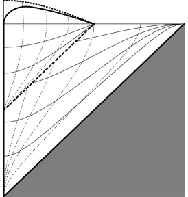
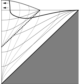
Figure 5: Toy conformal diagrams of a crunching bubble indicating the cutoff implied by the fat geodesic (left panel) and scale-factor cutoff (right panel) measures. The symbolism is the same as in Figure 1, but with the future boundary of the bubble given by a big-crunch singularity (thick, dotted line). The fat geodesic focuses on an arbitrarily small region surrounding a worldline at the left edge of the diagram, which grows to enclose a diverging conformal volume as the scale factor goes to zero. The cutoff implied by the scale-factor cutoff measure could enclose a smaller volume, depending on its definition, as indicated by the arrows.

In bubbles with positive vacuum energy, we expect the predictions of the SF+ measure to be very similar to those of the fat geodesic measure. Indeed, given the approximations of [2] (in particular, disregarding inhomogeneities caused by structure formation), they make the same predictions. Thus Figure 5 of [2] also describes the distribution of $\ell>0$ and $N$ for the SF+ measure, and we see there are no runaways. When $\ell$ is negative, the two measures make the same predictions during the expanding phase of bubble evolution, but differ after scale-factor turnaround. This can be seen by referring to Figure 5. Whereas the fat geodesic expands to enclose a diverging quantity of matter (when represented in the conformal diagram), the SF+ cutoff will enclose a finite quantity of matter, because that is all that remains along the defining congruence after the cutoff has been imposed outside of the crunching bubble. Thus, the SF+ measure is free of runaways in the $(\ell,N)$ plane.

5 Discussion and conclusions

Our goal in this paper was to investigate the phenomenological properties of the CAH+ measure. We found that this measure does not suffer from any known pathologies, such as the youngness paradox, $Q$ or $G$ catastrophes, or the Boltzmann brain problem (assuming that anthropic vacua in the landscape have sufficiently fast decay rates). The distribution for the cosmological constant $\Lambda$ derived from the CAH+ measure is in a good agreement with the observed value, and the distribution for the number of inflationary $e$-foldings $N$ satisfies the observational constraint. We found also that this measure assigns a non-negligible probability to a detectable negative curvature in the present universe. By its construction, the CAH+ measure satisfies the causality condition, requiring that the cutoff hypersurfaces should be spacelike or null.

The properties of the CAH+ measure are similar to those of the SF+ measure (that is, of the scale-factor measure with cutoff surfaces modified as in the ”+” prescription of this paper). In fact, of all the measures that have been discussed so far, these are the only two that agree with the available data and have no pathological features. In contrast, the causal patch, fat geodesic, and (local) apparent horizon cutoff measures give strong preference to negative values of $\Lambda$, and thus are in conflict with observations [2]. Restricting to positive values of $\Lambda$, the causal patch measure gives a non-normalizable distribution, diverging towards $\Lambda=0$. The divergence can be cut off due to the discrete character of the landscape, provided that there are no anthropic vacua with $\Lambda=0$. The maximum of the distribution is then shifted towards values comparable to the scale of discreteness, and the predicted value may be unfavorably affected by the jaggedness of the distribution on that scale. It should also be mentioned that all local measures are sensitive to the initial conditions and remain essentially undefined until the ensemble of initial states is specified.

For completeness, we mention some measures that have not been discussed in the main text. The proper time [39, 40, 42], pocket-based [14], and stationary [3] measures all suffer from $Q$ and $G$ catastrophes. In addition, the proper time measure is subject to the youngness paradox, and the pocket based measure to the Boltzmann brain problem.

Throughout this paper we assumed the spacetime to be $(3+1)$-dimensional. However, in general we expect the string theory landscape to allow parent vacua to nucleate daughter vacua with different effective dimensionality [49, 50, 51, 52]. Predictions of the scale factor cutoff measure in a transdimensional landscape have been studied in [53], with the conclusion that in cases when the highest number of spatial dimensions in inflating vacua is $D_{\rm max}>5$, this measure strongly disfavors large amounts of slow-roll inflation in the bubbles and predicts low values of the density parameter $\Omega$, in conflict with observations. This problem is avoided if instead of the scale factor measure one uses the volume factor (VF) cutoff, where the cutoff surfaces are surfaces of constant volume expansion factor. (These surfaces are the same as the constant scale factor surfaces in 3+1 dimensions, but are generally different in a transdimensional multiverse.) In order to comply with the causality condition, the modified VF+ measure can be defined by adding the “+” prescription.

The situation with the CAH+ measure is similar. It generally predicts low values of $\Omega$ in the transdimensional case. The analog of the VF+ measure in this case is the CNAH+ measure, in which the cutoff surfaces are the surfaces having a constant number of apparent horizons per equal comoving volume (with added “+” prescription). It is not presently clear how this measure can be related to a UV cutoff in the holographic boundary theory. This remains a topic for future research.

Appendix A Evolution of the CAH through CDL bubble nucleation

Here we compute the evolution of the CAH time $\theta$ along a congruence of timelike geodesics that begin in the parent vacuum and enter the bubble. Disregarding bubble collisions, the spacetime in the vicinity of a bubble can be represented by the spatially-flat de Sitter chart,

$$ds^{2}=-dt^{2}+e^{2H_{\rm p}t}\left(dr^{2}+r^{2}\,d\Omega_{2}^{2}\right),$$ (46)

where $H_{\rm p}$ is the parent-vacuum Hubble rate. We consider a congruence $\gamma_{r}$ of geodesics parametrized by $r=$ constant in the parent vacuum. As mentioned in the main text, the bubble geometry is of the form

$$ds^{2}=-d\tau^{2}+\overline{a}^{2}(\tau)\Big{[}d\xi^{2}+\sinh^{2}(\xi)\,d\Omega_{2}^{2}\Big{]}\,,$$ (47)

where here we focus exclusively on the scale-factor solution

$$\overline{a}(\tau)=H_{\rm d}^{-1}\,\sinh(H_{\rm d}\tau)\,.$$ (48)

We take the bubble to nucleate with a negligible initial radius at the parent-vacuum coordinates $(t,\,r)=(0,\,0)$, the future lightcone of which corresponds to the hypersurface $\tau=0$ in the bubble. Furthermore we work in the thin-wall approximation, with the bubble wall at the aforementioned future lightcone, and neglect any effect of bubble-wall tension on the trajectories of geodesics that pass through it.

To propagate the congruence $\gamma_{r}$ into the bubble, it will help to embed the spacetime in a (4+1)-dimensional Minkowski space, for which we write the line element

$$ds^{2}=-dT^{2}+dS^{2}+dR^{2}+R^{2}\,d\Omega_{2}^{2}\,.$$ (49)

The geometry of the parent vacuum is induced on the hyperboloid $-T^{2}+S^{2}+R^{2}=H_{\rm p}^{-2}$, which can be accomplished with the embedding

$$T = H_{\rm p}^{-1}\sinh(H_{\rm p}t)+\frac{1}{2}H_{\rm p}\,r^{2}\,e^{H_{\rm p}t}$$ (50)

$$S = H_{\rm p}^{-1}\cosh(H_{\rm p}t)-\frac{1}{2}H_{\rm p}\,r^{2}\,e^{H_{\rm p}t}$$ (51)

$$R = r\,e^{H_{\rm p}t}\,,\phantom{\frac{1}{2}}$$ (52)

where we have suppressed coordinates on the unit two-sphere, which do not concern us here. A general spacetime of the form (47) can also be embedded in Minkowski space, but for concreteness we focus on the specific, early-time solution (48). This can be embedded via

$$T = H_{\rm d}^{-1}\,\sinh(H_{\rm d}\tau)\cosh(\xi)$$ (53)

$$S = H_{\rm d}^{-1}\,\cosh(H_{\rm d}\tau)+H_{\rm p}^{-1}-H_{\rm d}^{-1}$$ (54)

$$R = H_{\rm d}^{-1}\,\sinh(H_{\rm d}\tau)\sinh(\xi)\,.$$ (55)

The bubble geometry then corresponds to that induced on the hyperboloid

$$-T^{2}+\big{(}S+H_{\rm d}^{-1}-H_{\rm p}^{-1}\big{)}^{2}+R^{2}=H_{\rm d}^{-2}\,,$$ (56)

which has been shifted from the origin so that it intersects the parent-vacuum hyperboloid at $S=H_{\rm p}^{-1}$, where we place the bubble wall. For the purpose of matching the two coordinate systems it is convenient to also introduce a spatially-flat de Sitter chart in the bubble. The line element is of the form (46), but with $H_{\rm p}\to H_{\rm d}$, and likewise the embedding is of the form (50)–(52), but with $H_{\rm p}\to H_{\rm d}$ followed by $S\to S+H_{\rm p}^{-1}-H_{\rm d}^{-1}$.

Our calculation of the propagation of the congruence $\gamma_{r}$ into the bubble follows the analysis of [54] (for more background see [55]). Figure 6 illustrates the dynamics, projected onto a conformal diagram of CDL bubble nucleation (the spatially-flat de Sitter chart of the parent vacuum covers only the upper-left half of the diagram). Initially-comoving geodesics (with respect to the spatially-flat parent-vacuum frame) encounter the bubble wall, are boosted with respect to the bubble coordinates, but nevertheless rapidly asymptote to comoving in the bubble FRW frame, due to redshifting during inflation in the bubble.

Figure 6: Two initially-comoving geodesics, $r_{1}$ and $r_{2}$ (dark, solid curves), propagating from the parent vacuum into the bubble. The bubble wall corresponds to the thick, dashed line; dotted lines correspond to constant-$t$ (constant-$\tau)$ surfaces, while solid lines correspond to constant-$r$ (constant-$\xi$) surfaces, in the parent vacuum (bubble).

In terms of the two spatially-flat charts, the trajectory of the bubble wall, specified by the intersection of the hypersurface $S=H_{\rm p}^{-1}$ with the two hyperboloids, is given by

$$H_{\rm p}r_{\rm w} = 1-e^{-H_{\rm p}t_{\rm w}}\,,\qquad H_{\rm p}t_{\rm w}=\ln(H_{\rm p}\,\lambda+1)\,,$$ (57)

$$H_{\rm d}\overline{r}_{\rm w} = 1-e^{-H_{\rm d}\overline{t}_{\rm w}}\,,\qquad H_{\rm d}\overline{t}_{\rm w}=\ln(H_{\rm d}\,\lambda+1)\,,$$ (58)

where we use overlines to denote coordinates in the spatially-flat chart within the bubble. The choice of parameter $\lambda$ is such that either trajectory maps to the same embedding coordinate $T$ (and, by definition, $S$) for a given value of $\lambda$.

Meanwhile, in terms of the spatially-flat slicing in the bubble, a general timelike geodesic (orthogonal to the unit two-sphere) takes the form

$$H_{\rm d}\overline{r} = H_{\rm d}\overline{r}_{\rm in}+\Big{(}v^{-2}+e^{-2H_{\rm d}\overline{t}_{\rm in}}\Big{)}^{\!1/2}-\,\Big{(}v^{-2}+e^{-2H_{\rm d}\overline{t}}\Big{)}^{\!1/2}$$ (59)

$$H_{\rm d}\overline{t} = \ln\!\left[v\sinh(H_{\rm d}s)\right],$$ (60)

where $(\overline{r}_{\rm in},\,\overline{t}_{\rm in})$ is the point along the bubble wall through which the geodesic passes, with $H_{\rm d}\overline{r}_{\rm in}=1-e^{-H_{\rm d}\overline{t}_{\rm in}}$ in accordance with (58), $v$ is an additional integration constant, and $s$ is the proper time along the geodesic. The coordinate $\overline{r}_{\rm in}$ of a geodesic just inside the bubble can be related to an element $r$ of the comoving congruence in the parent vacuum by matching the corresponding Minkowski embedding coordinates at the bubble wall. This gives

$$\overline{r}_{\rm in}=\frac{r}{1-H_{\rm p}r+H_{\rm d}r}\,.$$ (61)

The integration constant $v$ can be determined by equating the inner products between the geodesic and the normal to the bubble wall worldsheet, on either side of the wall. This gives

$$v=\frac{r\,(H_{\rm p}-H_{\rm d})(2-H_{\rm p}r+H_{\rm d}r)}{2\,(1-H_{\rm p}r)}\,.$$ (62)

We are now prepared to express the propagation of the congruence $\gamma_{r}$ into the bubble, in terms of the open–de Sitter chart (47)–(48) respecting the FRW symmetry of the bubble. The spatially-flat and open de Sitter charts can be related by identifying points on the hyperboloid in the Minkowski embedding space; this gives

$$e^{H_{\rm d}\overline{t}} = \cosh(H_{\rm d}\tau)+\sinh(H_{\rm d}\tau)\cosh(\xi)\phantom{\frac{1}{2}}$$ (63)

$$H_{\rm d}\overline{r} = \frac{\sinh(H_{\rm d}\tau)\sinh(\xi)}{\cosh(H_{\rm d}\tau)+\sinh(H_{\rm d}\tau)\cosh(\xi)}\,.$$ (64)

We see that at sufficiently late FRW times $\tau$, the spatially-flat coordinates become comoving with respect to the open coordinates (that is, $d\overline{r}/d\tau\to 0$), and we have

$$e^{H_{\rm d}\overline{t}}\,\to\,e^{H_{\rm d}\tau}\left[\frac{1}{2}+\frac{1}{2}\cosh(\xi)\right],\qquad H_{\rm d}\overline{r}\,\to\,\frac{\sinh(\xi)}{1+\cosh(\xi)}\,.$$ (65)

Since $\cosh(\xi)\geq 1$, the inequality $H_{\rm d}\tau\gg 1$ implies the inequality $H_{\rm d}\overline{t}\gg 1$. Meanwhile, for times $H_{\rm d}\overline{t}\gg 1$, the geodesic given by (59) and (60) asymptotes to evolution along a fixed value of the coordinate $\overline{r}$. Substituting (61) and (62) into (59), we find

$$H_{\rm d}\overline{r}\,\to\,\frac{H_{\rm p}r+H_{\rm d}r}{2-H_{\rm p}r+H_{\rm d}r}\,.$$ (66)

Expressing this in terms of the bubble coordinate $\xi$, we obtain

$$\xi\,\to\,\ln\!\left(\frac{1+H_{\rm d}r}{1-H_{\rm p}r}\right)\,.$$ (67)

With the dynamics of the geodesic congruence $\gamma_{r}$ in hand, we can now evolve the CAH time from deep within the parent vacuum to deep within the bubble. We first pick an “initial” constant-AH hypersurface $\Sigma_{0}$, which we take to coincide with the hypersurface $t=0$ in the parent vacuum. The scale factor is constant on this hypersurface, so it is also a surface of constant CAH, with $r_{\rm CAH}=r_{\rm AH}=H_{\rm p}^{-1}$. According to (67), a small, radial comoving coordinate separation $\Delta r$ in the spatially-flat de Sitter slicing of the parent vacuum translates into a comoving coordinate separation

$$\Delta\xi=\frac{(H_{\rm p}+H_{\rm d})\,\Delta r}{(1-H_{\rm p}r)(1+H_{\rm d}r)}=\frac{(H_{\rm p}+H_{\rm d}e^{-\xi})^{2}\,e^{\xi}\,\Delta r}{H_{\rm p}+H_{\rm d}}\,,$$ (68)

at times $H_{\rm d}\tau\gg 1$ in the bubble. To obtain the CAH in the bubble, we start with the AH radius $r_{\rm AH}=H_{\rm d}^{-1}$, divide by the bubble scale factor to convert to comoving coordinates, and then divide by $\left[\sinh^{2}(\xi)\,\Delta\xi/r^{2}\Delta r\right]^{1/3}$ to convert comoving bubble coordinates to comoving parent-vacuum coordinates on the “initial” hypersurface $\Sigma_{0}$. (Here we exploit the symmetries of an “annulus” centered at $r=\xi=0$ to compute the comoving volume expansion factor implied by the relation (67).) This gives the CAH time

$$\theta\equiv\frac{1}{r_{\rm CAH}}=\frac{\overline{a}(\tau)}{r_{\rm AH}}\left[\frac{\sinh^{2}(\xi)}{r^{2}(\xi)}\frac{\Delta\xi}{\Delta r}\right]^{1/3}\!=\,\left[\frac{(1+e^{-\xi})^{2}(H_{\rm p}+H_{\rm d}e^{-\xi})^{4}}{32\,(H_{\rm p}+H_{\rm d})}\right]^{1/3}e^{\xi+H_{\rm d}\tau}\,.$$ (69)

Note that the CAH time depends on $\xi$, rapidly increasing for large $\xi$, which is a necessary condition for the CAH cutoff to regulate the spacetime volume of the bubble, which is divergent on constant-$\tau$ hypersurfaces. Although $\theta$ is not constant (with respect to varying $\xi$) on surfaces of constant FRW proper time in the bubble, at late times this variation is small on any fixed distance scale. In particular, the AH scale $H_{\rm d}$ is covered by the comoving distance $\Delta\xi_{\rm AH}(\tau)=H_{\rm d}^{-1}\overline{a}^{-1}(\tau)$, and so

$$\frac{1}{\theta}\frac{d\theta}{d\xi}\Delta\xi_{\rm AH}=\frac{6H_{\rm p}+2(H_{\rm p}-H_{\rm d})e^{-\xi}-6H_{\rm d}e^{-2\xi}}{3\,(1+e^{-\xi})(H_{\rm p}+H_{\rm d}e^{-\xi})}\,e^{-H_{\rm d}\tau}\,,$$ (70)

which is very small when $H_{\rm d}\tau\gg 1$. This means that it was unnecessary to take the $t=0$ hypersurface as the “initial” constant-CAH surface with respect to which we define CAH time, as was done above. Since CDL bubbles in de Sitter vacua never expand beyond the (locally-defined) comoving AH, within the vicinity of any such bubble the spatially-flat de Sitter slicing serves as a constant CAH time foliation.

Equation (69) gives the result we are looking for: the CAH time $\theta\equiv r_{\rm CAH}^{-1}$ (relative to the CAH time on the hypersurface $t=0$ in the parent vacuum) at a given point in the bubble, deep in the inflationary epoch. The evolution of $\theta$ during a standard big bang cosmology after inflation is discussed in the main text. Note that if the vacuum energy in the parent vacuum is significantly larger than the inflationary energy density in the bubble, $H_{\rm p}\gg H_{\rm d}$, we obtain

$$\theta=\frac{1}{2}H_{\rm p}\left(\frac{1}{2}+\frac{1}{2}e^{-\xi}\right)^{\!2/3}e^{\xi+H_{\rm d}\tau}\,,$$ (71)

which is qualitatively accurate even for $H_{\rm p}$ rather near $H_{\rm d}$. The prefactor $H_{\rm p}$ can be understood to represent the CAH time on the initial hypersurface $t=0$ in the parent vacuum; had we chosen this hypersurface to reside at some earlier time $t=-t_{\rm n}$, this prefactor would have been $H_{\rm p}\,e^{H_{\rm p}t_{\rm n}}$. Meanwhile, the factor in parentheses is equal to one when $\xi=0$, and asymptotes to $2^{-2/3}\approx 0.63$ at large $\xi$. We therefore simply ignore this factor, to simplify the algebra without significantly changing the CAH time in the bubble. Accordingly, in the main text we write

$$\theta=\theta_{0}\,e^{H_{\rm p}t_{\rm n}+\xi+H_{\rm d}\tau}\,,$$ (72)

where $2\theta_{0}$ is the CAH time on the initial hypersurface $\Sigma_{0}$, taken to reside a proper time $t_{\rm n}$ before the point of bubble nucleation, along a comoving geodesic in the parent vacuum.

Appendix B Big bang cosmology

We here describe the scale-factor and growth-factor evolution in bubbles of interest. We assume an initial period of curvature domination, in accordance with matching CDL boundary conditions at FRW proper time $\tau=0$ (conformal time $\eta\to-\infty$), followed by inflation (approximated as constant vacuum-energy domination), instantaneous reheating yielding radiation domination, non-relativistic matter domination, spatial-curvature domination (again), and/or cosmological-constant domination. With respect to scale-factor evolution, in (almost) every case we approximate the transition between these periods as instantaneous, solving the Einstein field equation $H^{2}=(8\pi G/3)\,\rho$ and the Friedmann equation $\dot{\rho}=-3H(\rho+p)$ for a perfect fluid with the appropriate equation of state $w=p/\rho$ (for energy density $\rho$ and pressure density $p$), and setting the integration constants so as to make the scale factor $\overline{a}$ and its first time derivative continuous across the transition. Approximating the growth-factor evolution involves a bit more finesse, described below.

B.1 Scale factor evolution

From FRW proper time $\tau=0$ up until the end of inflation, we take the scale factor to be

$$\overline{a}(\tau)=H_{\rm d}^{-1}\sinh(H_{\rm d}\tau)\,\to\,\frac{1}{2H_{\rm d}}e^{H_{\rm d}\tau}\,,$$ (73)

where here and below the arrows indicate the late time limits, which in each case we take to be accurate approximations for matching the scale factor onto the next phase of its evolution. As usual, conformal time is defined $\int d\tau/\overline{a}(\tau)$; so that at late times we have

$$\overline{a}(\eta)\,\to\,-\frac{1}{H_{\rm d}\eta}\,,\qquad\eta\,\to\,-2e^{-H_{\rm d}\tau}\,.$$ (74)

We assume instantaneous reheating, and thus match directly onto the scale-factor evolution during radiation domination ($w=1/3$). This gives

$$\overline{a}(\tau)=e^{N}\left(\frac{\tau}{2H_{\rm d}}-\frac{2N-1}{4H_{\rm d}^{2}}\right)^{\!1/2}\to\,e^{N}\left(\frac{\tau}{2H_{\rm d}}\right)^{\!1/2}\,.$$ (75)

In terms of conformal time, the late-time limit corresponds to

$$\overline{a}(\eta)\,\to\,\frac{1}{4H_{\rm d}}\,e^{2N}\eta\,,\qquad\eta\,\to\,e^{-N}(8H_{\rm d}\tau)^{1/2}\,.$$ (76)

The above period of radiation domination gives way to a period of non-relativistic matter domination ($w=0$), and we denote the time of the transition $\tau_{\rm eq}$. The actual value of $\tau_{\rm eq}$ is given by microphysical parameters and will not by itself be important to our results. Matching the scale-factor evolution as described above, we find

$$\overline{a}(\tau)=\frac{e^{N}(3\tau+\tau_{\rm eq})^{2/3}}{2^{11/6}\,H_{\rm d}^{1/2}\tau_{\rm eq}^{1/6}}\,\to\,\frac{3^{2/3}\,e^{N}\,\tau^{2/3}}{2^{11/6}\,H_{\rm d}^{1/2}\,\tau_{\rm eq}^{1/6}}\,.$$ (77)

In hindsight, we recognize that the above combination of factors is proportional to the time of the transition to spatial-curvature domination (in bubbles where the number of $e$-folds of inflation is such that this precedes cosmological-constant domination), which we here note is

$$\tau_{\rm c}=\frac{e^{3N}}{3\!\cdot\!2^{5/2}H_{\rm d}^{3/2}\tau_{\rm eq}^{1/2}}\,,\qquad{\rm so\,\,that}\qquad\overline{a}(\tau)\,\to\frac{3}{2}\tau_{\rm c}^{1/3}\tau^{2/3}\,.$$ (78)

In terms of conformal time, the late-time limit corresponds to

$$\overline{a}(\eta)\,\to\,\frac{3}{8}\tau_{\rm c}\eta^{2}\,,\qquad\eta\,\to\,2\tau_{\rm c}^{-1/3}\tau^{1/3}\,.$$ (79)

Non-relativistic matter domination persists until spatial-curvature or cosmological-constant domination, at time $\tau_{\rm c}$ or $\tau_{\rm\Lambda}$. In the first case we treat the spatial curvature as a perfect fluid with energy density $\overline{a}^{-2}$ and equation of state $w=-1/3$. Matching onto the previous scale-factor evolution then gives

$$\overline{a}(\tau)=\tau+\frac{1}{2}\tau_{\rm c}\,\to\,\tau\,.$$ (80)

The time of the transition can be obtained by solving for when the Hubble rate implied by (78) is equal to the Hubble rate implied by (80), which confirms the result introduced with hindsight above. In terms of conformal time, we have

$$\overline{a}(\eta)=\frac{3}{2}\tau_{\rm c}\,e^{\eta-2}\,,\qquad\eta=2+\ln\!\left(\frac{2}{3}\frac{\tau}{\tau_{\rm c}}+\frac{1}{3}\right).$$ (81)

If the cosmological constant is precisely zero, the scale factor evolves according to the above curvature-dominated results all the way to future infinity. Meanwhile, for positive cosmological constant the scale factor is given by

$$\overline{a}(\tau)=H_{\Lambda}^{-1}e^{H_{\Lambda}\tau+\frac{1}{2}H_{\Lambda}\tau_{\rm c}-1}\,,$$ (82)

where $H_{\Lambda}\equiv(|\Lambda|/3)^{1/2}$ (the absolute value being introduced for later convenience). Note that the transition from curvature to cosmological-constant domination occurs at $\tau_{\Lambda}\equiv H_{\Lambda}^{-1}-\tau_{\rm c}/2$. In terms of conformal time, we have

$$\overline{a}(\eta)=H_{\Lambda}^{-1}\!\left[3-\ln\!\left(\textstyle\frac{3}{2}H_{\Lambda}\tau_{\rm c}\right)-\eta\right]^{-1},\quad\eta=3-\ln\!\left(\textstyle\frac{3}{2}H_{\Lambda}\tau_{\rm c}\right)-e^{-H_{\Lambda}\tau-\frac{1}{2}H_{\Lambda}\tau_{\rm c}+1}\,.$$ (83)

When the cosmological constant is negative, it is not possible to proceed as above and model FRW scale factor evolution as if the cosmological constant were the only important contribution to the energy density. Therefore, for this case we include both spatial curvature and cosmological constant in the Einstein field equation. The solution that matches onto the scale-factor evolution at the end of matter domination for generic parameters $\tau_{\rm c}$ and $H_{\Lambda}$ involves a complicated integration constant. Therefore we use the approximation

$$a(\tau)=H_{\Lambda}^{-1}\sin\!\Big{[}H_{\Lambda}(\tau-\tau_{\rm c})+\arcsin\!\left(\textstyle\frac{3}{2}H_{\Lambda}\tau_{\rm c}\right)\Big{]},$$ (84)

for which the scale factor is continuous at $\tau=\tau_{\rm c}$ for generic parameters, and smooth when $\tau_{\rm c}\ll H_{\Lambda}^{-1}$. This approximation for the phase of the sine function becomes poorer as the product $H_{\Lambda}\tau_{\rm c}$ approaches 2/3 (when $H_{\Lambda}\tau_{\rm c}$ is larger than this we use another solution for the scale factor), however the discrepancy becomes unimportant as $\tau$ becomes much larger than $\tau_{\rm c}$. In terms of conformal time, we have

$$\overline{a}(\eta) = H_{\Lambda}^{-1}\sin\!\bigg{[}2\arctan\left\{e^{\eta-2}\tan\!\left[\frac{1}{2}\arcsin\!\left(\textstyle\frac{3}{2}H_{\Lambda}\tau_{\rm c}\right)\right]\right\}\bigg{]}$$ (85)

$$\eta = 2+\ln\!\left\{\tan\!\left[\frac{1}{2}H_{\Lambda}(\tau-\tau_{\rm c})+\frac{1}{2}\arcsin\!\left(\textstyle\frac{3}{2}H_{\Lambda}\tau_{\rm c}\right)\right]\cot\!\left[\frac{1}{2}\arcsin\!\left(\textstyle\frac{3}{2}H_{\Lambda}\tau_{\rm c}\right)\right]\right\}.\,\,\,\,$$ (86)

After the onset of negative cosmological-constant domination, the scale factor eventually stops growing and subsequently decreases with time. The subsequent evolution then corresponds to the time reversal of the evolution described above, reflected about the “turnaround” time

$$\tau_{\rm turn}=\tau_{\rm c}+\frac{\pi}{2H_{\Lambda}}-H_{\Lambda}^{-1}\arcsin\!\left(\textstyle\frac{3}{2}H_{\Lambda}\tau_{\rm c}\right)\,,\quad\eta_{\rm turn}=2+\ln\!\left\{\cot\!\left[\frac{1}{2}\arcsin\!\left(\textstyle\frac{3}{2}H_{\Lambda}\tau_{\rm c}\right)\right]\right\}.$$ (87)

If non-relativistic matter domination gives way directly to positive cosmological-constant domination, then the scale-factor evolution can be written

$$\overline{a}(\tau)=\left(\frac{3\tau_{\rm c}}{2H_{\Lambda}^{2}}\right)^{\!1/3}\,e^{H_{\Lambda}\tau-2/3}\,,$$ (88)

where in this context (i.e. when there is no epoch of late-time spatial-curvature domination) the transition time is given by $\tau_{\Lambda}=(2/3)H_{\Lambda}^{-1}$. Whether or not there is a period of spatial-curvature domination between non-relativistic matter domination and cosmological-constant domination depends on whether or not this $\tau_{\Lambda}$ is greater than $\tau_{\rm c}$; thus there is no epoch of late-time curvature domination when $\tau_{\rm c}>(2/3)H_{\Lambda}^{-1}$. Proceeding, we write the above solution in terms of conformal time,

$$\overline{a}(\eta)=H_{\Lambda}^{-1}\bigg{[}\left(\textstyle\!\frac{1}{18}H_{\Lambda}\tau_{\rm c}\right)^{\!-1/3}\!-\,\eta\bigg{]}^{-1},\qquad\eta=\left(\textstyle\frac{3}{2}H_{\Lambda}\tau_{\rm c}\right)^{\!-1/3}\left(3-e^{-H_{\Lambda}\tau+2/3}\right)\,.$$ (89)

When the cosmological constant is negative, we run into the same problem as before. Therefore, for this case we include both non-relativistic matter and cosmological constant in the Einstein field equation. Since we are ultimately only interested in periods after non-relativistic matter domination in cosmologies with $\tau_{\rm eq}\ll H_{\Lambda}^{-1}$, we can simply take the solution

$$\overline{a}(\tau)=\left(\frac{3\tau_{\rm c}}{2H_{\Lambda}^{2}}\right)^{\!1/3}\sin^{2/3}\!\left(\frac{3}{2}H_{\Lambda}\tau\right),$$ (90)

which matches onto the late-time non-relativistic matter domination solution in the small-time limit. The scale-factor solution in terms of conformal time can be approximated by combining (90) with the inversion of

$$\eta=-\left(\frac{2}{3H_{\Lambda}\tau_{\rm c}}\right)^{\!1/3}\left\{\frac{2\pi^{3/2}}{\Gamma(-\frac{1}{3})\,\Gamma(\frac{5}{6})}+\frac{2}{3}\cos\!\left(\frac{3}{2}H_{\Lambda}\tau\right)F\!\left[\frac{1}{2},\,\frac{5}{6},\,\frac{3}{2},\,\cos^{2}\!\left(\frac{3}{2}H_{\Lambda}\tau\right)\right]\right\},$$ (91)

where $F$ is the hypergeometric function, and we have again used $\tau_{\rm eq}\ll H_{\Lambda}^{-1}$ to drop subleading terms. As in the case where there is a period of spatial-curvature domination, negative cosmological-constant domination gives way to turnaround followed by the time reversal of the previous scale-factor evolution. In this case the turnaround time is given by

$$\tau_{\rm turn}=\frac{\pi}{3H_{\Lambda}}\,,\qquad\eta_{\rm turn}=-\frac{2\pi^{3/2}}{\Gamma(-\frac{1}{3})\,\Gamma(\frac{5}{6})}\left(\frac{2}{3H_{\Lambda}\tau_{\rm c}}\right)^{\!1/3}\,.$$ (92)

B.2 Growth factor evolution

In the linear approximation, a spherical top-hat overdensity in non-relativistic matter obeys the equation of motion (see for example [56])

$$\ddot{\sigma}+2H\dot{\sigma}-\frac{9}{4}\frac{\tau_{\rm c}}{\overline{a}^{3}}\sigma=0\,,$$ (93)

where $\sigma\equiv\delta\rho_{\rm m}/\rho_{\rm m}$ and we have used that the non-relativistic matter density can be written $\rho_{\rm m}=(3/2)\tau_{\rm c}/\overline{a}^{3}$. The primordial density perturbations in bubbles like ours are nearly scale invariant and at least approximately Gaussian; we are interested in the root-mean-square (rms) density contrast averaged over a comoving scale enclosing a mass $M$ of non-relativistic matter. It is customary to separate this quantity into two parts, writing

$$\sigma_{\rm rms}(M,\tau)=\sigma_{\rm ref}(M)\,D(\tau)\,,$$ (94)

where $\sigma_{\rm ref}$ is the rms density contrast evaluated at some reference time $\tau_{\rm ref}$, which we take to be deep into the period of non-relativistic matter domination, and $D$ is the growth factor, describing the evolution of $\sigma$ after that. We fix $\sigma_{\rm ref}$ to match observation [32].

It is customary to use the linearized equations of motion to determine the growth factor $D$ even after perturbations have grown so large as to make the linear approximation inappropriate, and to account for this convention separately (see the main text). When the bubble can be approximated as containing only non-relativistic matter, spatial curvature, and cosmological constant, (93) admits the solution [56]

$$D(\overline{a})=\frac{5}{2}\left(\frac{\tau_{\rm c}}{\tau_{\rm ref}}\right)^{\!2/3}\left(\frac{\gamma^{3}}{H_{\Lambda}^{3}\overline{a}^{3}}+\frac{1}{H_{\Lambda}^{2}\overline{a}^{2}}\pm 1\right)^{\!1/2}\left[C+\int_{0}^{H_{\Lambda}\overline{a}}dx\left(\frac{\gamma^{3}}{x}+1\pm x^{2}\right)^{\!-3/2}\right],$$ (95)

where $\gamma\equiv(\frac{3}{2}H_{\Lambda}\tau_{\rm c})^{1/3}$, $\pm$ corresponds to the sign of the cosmological constant, and $C$ is an integration constant. The constant $C$ is unimportant at times $\tau\gg\tau_{\rm ref}$, and can therefore be set to zero, except after scale-factor turnaround in bubbles with negative cosmological constant. In that case $C$ is determined by demanding that $dD/d\tau$ is continuous at turnaround (the form of (95) guarantees that it is continuous at turnaround). Formally, this gives

$$C = \lim_{\overline{a}\to\overline{a}_{\rm turn}}\Bigg{\{}\!\left(\frac{3}{4}\frac{\gamma^{3}}{H_{\Lambda}\overline{a}}+\frac{1}{2}\right)^{\!-1}\!\left(\frac{\gamma^{3}}{H_{\Lambda}^{3}\overline{a}^{3}}+\frac{1}{H_{\Lambda}^{2}\overline{a}^{2}}-1\right)^{\!-1/2}$$ (96)

$$\qquad\quad\,\,-\,2\int_{0}^{H_{\Lambda}\overline{a}}dx\left(\frac{\gamma^{3}}{x}+1-x^{2}\right)^{\!-3/2}\Bigg{\}},$$

where $\overline{a}_{\rm turn}$ is the value of the scale factor at turnaround. The divergence in the first term is canceled by a divergence in the integral, when the expressions are regulated.

Unfortunately, we cannot obtain a closed-form expression for the integral in (95). Nevertheless, a bit of trial and error allows us to find a set of results that reasonably approximate $D$. To begin, we focus on bubbles with positive cosmological constant, and divide the integration over $x$ into two parts: one for which the sum $\gamma^{3}/x+1$ dominates the integrand (corresponding to the effects of non-relativistic matter and spatial curvature dominating the Hubble rate), the other for which the sum $1+x^{2}$ dominates the integrand (corresponding to the effects of spatial curvature and cosmological constant dominating the Hubble rate). These two parts are matched at $x=\gamma$, which corresponds to when the energy density in non-relativistic matter is equal to the energy density in cosmological constant. Accordingly, for $H_{\Lambda}\overline{a}<(\frac{3}{2}H_{\Lambda}\tau_{\rm c})^{1/3}$, in which case $x<\gamma$ over the entire range of integration, we write

$$D(\overline{a}) = \frac{5}{2}\left(\frac{\tau_{\rm c}}{\tau_{\rm ref}}\right)^{\!2/3}\left(\frac{\gamma^{3}}{H_{\Lambda}^{3}\overline{a}^{3}}+\frac{1}{H_{\Lambda}^{2}\overline{a}^{2}}\right)^{\!1/2}\int_{0}^{H_{\Lambda}\overline{a}}dx\left(\frac{\gamma^{3}}{x}+1\right)^{\!-3/2}$$ (97)

$$= \frac{5}{2}\left(\frac{\tau_{\rm c}}{\tau_{\rm ref}}\right)^{\!2/3}\Bigg{\{}1+\frac{3\gamma^{3}}{H_{\Lambda}\overline{a}}-\frac{3\gamma^{3}}{H_{\Lambda}\overline{a}}\left(1+\frac{\gamma^{3}}{H_{\Lambda}\overline{a}}\right)^{\!1/2}{\rm arcsinh}\!\left[\frac{(H_{\Lambda}\overline{a})^{1/2}}{\gamma^{3/2}}\right]\!\Bigg{\}}\,,$$

where the prefactor $H(\overline{a})/H_{\Lambda}$ has been modified from (95), in accordance with the above approximation, to improve accuracy and provide continuity in the full result. Meanwhile, for $H_{\Lambda}\overline{a}\geq(\frac{3}{2}H_{\Lambda}\tau_{\rm c})^{1/3}$ we write

$$D(\overline{a}) = \frac{5}{2}\left(\frac{\tau_{\rm c}}{\tau_{\rm ref}}\right)^{\!2/3}\left(\frac{1}{H_{\Lambda}^{2}\overline{a}^{2}}+1\right)^{\!1/2}\Bigg{\{}\int_{0}^{\gamma}dx\left(\frac{\gamma^{3}}{x}+1\right)^{\!\!-3/2}\!+\int_{\gamma}^{H_{\Lambda}\overline{a}}dx\left(\gamma^{2}+1+x^{2}\right)^{\!-3/2}\Bigg{\}}$$ (98)

$$= \frac{5}{2}\left(\frac{\tau_{\rm c}}{\tau_{\rm ref}}\right)^{\!2/3}\left(\frac{1}{H_{\Lambda}^{2}\overline{a}^{2}}+1\right)^{\!1/2}\Bigg{\{}\frac{3\gamma^{3}+\gamma}{(\gamma^{2}+1)^{1/2}}-3\gamma^{3}{\rm arcsinh}\!\left(\gamma^{-1}\right)$$

$$+\,\frac{\gamma^{1/2}}{\gamma^{2}+1}\left[\frac{H_{\Lambda}\overline{a}}{\big{(}\gamma^{3}+\gamma+\gamma H_{\Lambda}^{3}\overline{a}^{3}\big{)}^{1/2}}-\frac{\gamma^{1/2}}{\big{(}2\gamma^{2}+1\big{)}^{1/2}}\right]\!\Bigg{\}}\,,$$

where we have added the term $\gamma^{2}$ to the second integrand because it significantly improves the accuracy of the approximation.

The case of negative cosmological constant is treated similarly. Indeed, we do not significantly increase the error if we compute $D(\overline{a})$ as if the cosmic fluid contained only non-relativistic matter and spatial curvature all the way up to scale-factor turnaround (of course we continue to use the scale factor solution that includes the effect of negative cosmological constant). This gives (97), now with the understanding that the result applies only for $\tau\leq\tau_{\rm turn}$. For later times, we incorporate the integration constant $C$ mentioned above. However, due to the present approximation, $D(\overline{a})$ is not continuous at $\overline{a}_{\rm turn}$ for any given value of $C$, so we set $C$ to the particular value for which the solution is continuous. This gives, for $\tau>\tau_{\rm turn}$,

$$D(\overline{a}) = \frac{5}{2}\left(\frac{\tau_{\rm c}}{\tau_{\rm ref}}\right)^{\!2/3}\left(\frac{\gamma^{3}}{H_{\Lambda}^{3}\overline{a}^{3}}+\frac{1}{H_{\Lambda}^{2}\overline{a}^{2}}\right)^{\!1/2}\Bigg{\{}\frac{2+6\gamma^{3}}{\left(1+\gamma^{3}\right)^{1/2}}-\left(\frac{\gamma^{3}}{H_{\Lambda}^{3}\overline{a}^{3}}+\frac{1}{H_{\Lambda}^{2}\overline{a}^{2}}\right)^{\!-1/2}$$ (99)

$$-\,3\gamma^{3}\left(1+\frac{\gamma^{3}}{H_{\Lambda}\overline{a}}\right)^{\!-1/2}\!\!-6\gamma^{3}{\rm arcsinh}\big{(}\gamma^{-3/2}\big{)}+3\gamma^{3}{\rm arcsinh}\!\left[\frac{(H_{\Lambda}\overline{a})^{1/2}}{\gamma^{3/2}}\right]\!\Bigg{\}}.\,\,\,\,$$

The case where non-relativistic matter domination gives way directly to cosmological-constant domination is included in the analysis above, as the limit of large $\gamma$. For sufficiently large $\gamma$, however, it is worthwhile to consider a different approximation, which improves the accuracy, especially with respect to the asymptotic value of $D$. Since for large $\gamma$ spatial curvature never contributes significantly to the post-inflationary energy density, to approximate this case we simply ignore the corresponding terms in (95). This gives

$$D(\overline{a}) = \frac{5}{2}\left(\frac{\tau_{\rm c}}{\tau_{\rm ref}}\right)^{\!2/3}\left(\frac{\gamma^{3}}{H_{\Lambda}^{3}\overline{a}^{3}}\pm 1\right)^{\!1/2}\int_{0}^{H_{\Lambda}\overline{a}}dx\left(\frac{\gamma^{3}}{x}\pm x^{2}\right)^{\!-3/2}$$ (100)

$$= \left(\frac{\tau_{\rm c}}{\tau_{\rm ref}}\right)^{\!2/3}\frac{H_{\Lambda}\overline{a}}{\gamma^{3}}\left(1\pm\frac{H_{\Lambda}^{3}\overline{a}^{3}}{\gamma^{3}}\right)^{\!-1/2}\Bigg{\{}\frac{8}{3}\,F\!\left(-\frac{1}{2},\,\frac{5}{6},\,\frac{11}{6},\,\mp\frac{H_{\Lambda}^{3}\overline{a}^{3}}{\gamma^{3}}\right)\quad$$

$$-\left(\frac{5}{3}\pm\frac{2H_{\Lambda}^{3}\overline{a}^{3}}{3\gamma^{3}}\right)F\!\left(\frac{1}{2},\,\frac{5}{6},\,\frac{11}{6},\,\mp\frac{H_{\Lambda}^{3}\overline{a}^{3}}{\gamma^{3}}\right)\!\Bigg{\}}\,,$$

where again $F$ denotes the hypergeometric function, and the upper (lower) entry of $\pm$ and $\mp$ corresponds to positive (negative) cosmological constant. In the case $\Lambda<0$, the solution above corresponds to $D$ before scale-factor turnaround. The solution after turnaround is obtained by incorporating an integration constant, as described below (95), except in the present approximation we drop the terms associated with spatial curvature. This gives

$$D(\overline{a}) = \frac{5}{2}\left(\frac{\tau_{\rm c}}{\tau_{\rm ref}}\right)^{\!2/3}\frac{H_{\Lambda}\overline{a}}{\gamma^{3}}\left(1-\frac{H_{\Lambda}^{3}\overline{a}^{3}}{\gamma^{3}}\right)^{\!-1/2}\Bigg{\{}\frac{4\sqrt{\pi}\,\Gamma(\frac{5}{6})}{3\,\Gamma(\frac{1}{3})}\frac{\gamma}{H_{\Lambda}\overline{a}}\left(\frac{\gamma^{3}}{H_{\Lambda}^{3}\overline{a}^{3}}+\frac{H_{\Lambda}^{3}\overline{a}^{3}}{\gamma^{3}}-2\right)^{\!1/2}$$ (101)

$$+\,\frac{8}{3}\,F\!\left(-\frac{1}{2},\,\frac{5}{6},\,\frac{11}{6},\,\frac{H_{\Lambda}^{3}\overline{a}^{3}}{\gamma^{3}}\right)-\left(\frac{5}{3}-\frac{2H_{\Lambda}^{3}\overline{a}^{3}}{3\gamma^{3}}\right)F\!\left(\frac{1}{2},\,\frac{5}{6},\,\frac{11}{6},\,\frac{H_{\Lambda}^{3}\overline{a}^{3}}{\gamma^{3}}\right)\!\Bigg{\}}\,.$$

Although the scale-factor solution of the previous section ignores the effect of spatial curvature for what corresponds to $\gamma\geq 1$, in the present setting it increases the accuracy of the approximation to use (100) only for $\gamma\geq 1.9$ when $\Lambda>0$.

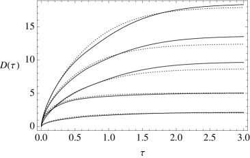
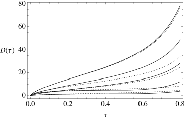
Figure 7: Comparison of two methods to compute the growth factor $D(\tau)$, (1) using the approximations developed in this appendix (solid curves) and (2) numerically integrating the linear evolution equation (dotted curves), for positive (left panel, where time is given in units of $H_{\Lambda}^{-1}$) and negative (right panel, where time is given in units of $\tau_{\rm turn}$) cosmological constant, and several values of $\gamma^{3}$: 0.1 (second from bottom), 0.5 (bottom), 2.0 (middle), 10 (second from top), and 100 (top). Some pairs of curves been r escaled to increase clarity.

It is not difficult to numerically check the accuracy of the above approximations against (95), since aside from a common prefactor, they can all be expressed as functions of $x=H_{\Lambda}\overline{a}$, involving only one additional parameter $\gamma$. The approximations are poorest for $\gamma\sim{\cal O}(1)$; several representative curves from this region of the parameter space are displayed in Figure 7. Since some error is introduced by the approximations used to determine the scale-factor $\overline{a}$, in Figure 7 we compare two methods to determine $D(\tau)$ (as opposed to $D(\overline{a})$). One method combines (95) with the numerically-integrated Einstein field equation,

$$H_{\Lambda}\tau=\int_{0}^{H_{\Lambda}\overline{a}}dx\left(\frac{\gamma}{x}+1+x^{2}\right)^{\!1/2},$$ (102)

inverted to give $\overline{a}(\tau)$. The other is the method outlined above, using the approximations for $\overline{a}(\tau)$ described in the previous subsection. Although the fits are not perfect, they are sufficient given the other uncertainties in our analysis, and they rapidly improve as $\gamma$ becomes very large or very small. (Note that because $\gamma\propto e^{N}$, the approximations are poorest only very near special values of $N$, and the curves of Figure 7 survey near those special values.)

Throughout the main text we use only the closed-form approximations for the growth function $D(\overline{a})$, in conjunction with the closed-form scale-factor solutions $\overline{a}(\tau)$ presented in the previous subsection, as opposed to the more computationally intensive numerical evaluations to which they are compared in Figure 7.

References

- [1] A. De Simone, A. H. Guth, A. D. Linde, M. Noorbala, M. P. Salem, A. Vilenkin, “Boltzmann brains and the scale-factor cutoff measure of the multiverse,” Phys. Rev. D82, 063520 (2010). [arXiv:0808.3778 [hep-th]].
- [2] R. Bousso, B. Freivogel, S. Leichenauer, V. Rosenhaus, “A geometric solution to the coincidence problem, and the size of the landscape as the origin of hierarchy,” Phys. Rev. Lett. 106, 101301 (2011). [arXiv:1011.0714 [hep-th]]; R. Bousso, B. Freivogel, S. Leichenauer, V. Rosenhaus, “Geometric origin of coincidences and hierarchies in the landscape,” [arXiv:1012.2869 [hep-th]].
- [3] A. D. Linde, V. Vanchurin, S. Winitzki, “Stationary Measure in the Multiverse,” JCAP 0901, 031 (2009). [arXiv:0812.0005 [hep-th]].
- [4] Y. Nomura, “Physical Theories, Eternal Inflation, and Quantum Universe,” [arXiv:1104.2324 [hep-th]].
- [5] B. Freivogel, “Making predictions in the multiverse,” [arXiv:1105.0244 [hep-th]].
- [6] J. Garriga and A. Vilenkin, “Holographic Multiverse,” JCAP 0901, 021 (2009) [arXiv:0809.4257 [hep-th]].
- [7] J. Garriga, A. Vilenkin, “Holographic multiverse and conformal invariance,” JCAP 0911, 020 (2009). [arXiv:0905.1509 [hep-th]].
- [8] R. Bousso, “Complementarity in the Multiverse,” Phys. Rev. D 79, 123524 (2009) [arXiv:0901.4806 [hep-th]].
- [9] R. Bousso, B. Freivogel, S. Leichenauer, V. Rosenhaus, “Boundary definition of a multiverse measure,” Phys. Rev. D82, 125032 (2010). [arXiv:1005.2783 [hep-th]].
- [10] A. Vilenkin, “Holographic multiverse and the measure problem,” arXiv:1103.1132 [hep-th].
- [11] R. Bousso, “The Holographic principle,” Rev. Mod. Phys. 74, 825-874 (2002). [hep-th/0203101].
- [12] S. R. Coleman, F. De Luccia, “Gravitational Effects on and of Vacuum Decay,” Phys. Rev. D21, 3305 (1980).
- [13] J. Garriga, A. Vilenkin, “Recycling universe,” Phys. Rev. D57, 2230-2244 (1998). [astro-ph/9707292].
- [14] J. Garriga, D. Schwartz-Perlov, A. Vilenkin, S. Winitzki, “Probabilities in the inflationary multiverse,” JCAP 0601, 017 (2006). [arXiv:hep-th/0509184 [hep-th]].
- [15] A. De Simone, A. H. Guth, M. P. Salem, A. Vilenkin, “Predicting the cosmological constant with the scale-factor cutoff measure,” Phys. Rev. D78, 063520 (2008). [arXiv:0805.2173 [hep-th]].
- [16] R. Bousso, B. Freivogel, I-S. Yang, “Properties of the scale factor measure,” Phys. Rev. D79, 063513 (2009). [arXiv:0808.3770 [hep-th]].
- [17] B. Feldstein, L. J. Hall, T. Watari, “Density perturbations and the cosmological constant from inflationary landscapes,” Phys. Rev. D72, 123506 (2005). [hep-th/0506235].
- [18] J. Garriga, A. Vilenkin, “Anthropic prediction for Lambda and the Q catastrophe,” Prog. Theor. Phys. Suppl. 163, 245-257 (2006). [hep-th/0508005].
- [19] M. L. Graesser, M. P. Salem, “The scale of gravity and the cosmological constant within a landscape,” Phys. Rev. D76, 043506 (2007). [astro-ph/0611694].
- [20] L. Dyson, M. Kleban, L. Susskind, “Disturbing implications of a cosmological constant,” JHEP 0210, 011 (2002). [hep-th/0208013].
- [21] A. Albrecht, L. Sorbo, “Can the universe afford inflation?,” Phys. Rev. D70, 063528 (2004). [hep-th/0405270].
- [22] D. N. Page, “Is our universe likely to decay within 20 billion years?,” Phys. Rev. D78, 063535 (2008). [hep-th/0610079].
- [23] R. Bousso, B. Freivogel, “A Paradox in the global description of the multiverse,” JHEP 0706, 018 (2007). [hep-th/0610132].
- [24] A. Vilenkin, “Predictions from quantum cosmology,” Phys. Rev. Lett. 74, 846-849 (1995). [gr-qc/9406010].
- [25] J. Garriga, A. Vilenkin, “Prediction and explanation in the multiverse,” Phys. Rev. D77, 043526 (2008). [arXiv:0711.2559 [hep-th]].
- [26] W. H. Press and P. Schechter, “Formation of galaxies and clusters of galaxies by selfsimilar gravitational condensation,” Astrophys. J. 187 (1974) 425; J. M. Bardeen, J. R. Bond, N. Kaiser and A. S. Szalay, “The Statistics Of Peaks Of Gaussian Random Fields,” Astrophys. J. 304, 15 (1986).
- [27] S. Weinberg, “Anthropic Bound on the Cosmological Constant,” Phys. Rev. Lett. 59, 2607 (1987).
- [28] D. Schwartz-Perlov, A. Vilenkin, “Probabilities in the Bousso-Polchinski multiverse,” JCAP 0606, 010 (2006). [hep-th/0601162].
- [29] K. D. Olum, D. Schwartz-Perlov, “Anthropic prediction in a large toy landscape,” JCAP 0710, 010 (2007). [arXiv:0705.2562 [hep-th]].
- [30] D. Schwartz-Perlov, “Anthropic prediction for a large multi-jump landscape,” JCAP 0810, 009 (2008). [arXiv:0805.3549 [hep-th]].
- [31] B. Freivogel, M. Kleban, M. Rodriguez Martinez and L. Susskind, “Observational consequences of a landscape,” JHEP 0603, 039 (2006) [arXiv:hep-th/0505232].
- [32] E. Komatsu et al. [WMAP Collaboration], “Seven-Year Wilkinson Microwave Anisotropy Probe (WMAP) Observations: Cosmological Interpretation,” Astrophys. J. Suppl. 192, 18 (2011) [arXiv:1001.4538 [astro-ph.CO]].
- [33] A. De Simone and M. P. Salem, “The distribution of from the scale-factor cutoff measure,” Phys. Rev. D 81, 083527 (2010) [arXiv:0912.3783 [hep-th]].
- [34] T. P. Waterhouse, J. P. Zibin, “The cosmic variance of Omega,” [arXiv:0804.1771 [astro-ph]].
- [35] M. Vardanyan, R. Trotta, J. Silk, “How flat can you get? A model comparison perspective on the curvature of the Universe,” Mon. Not. Roy. Astron. Soc. 397, 431-444 (2009). [arXiv:0901.3354 [astro-ph.CO]].
- [36] M. Tegmark, “What does inflation really predict?,” JCAP 0504, 001 (2005). [astro-ph/0410281].
- [37] A. H. Guth, “Eternal inflation and its implications,” J. Phys. A A40, 6811-6826 (2007). [hep-th/0702178 [HEP-TH]].
- [38] R. Bousso, B. Freivogel, I-S. Yang, “Boltzmann babies in the proper time measure,” Phys. Rev. D77, 103514 (2008). [arXiv:0712.3324 [hep-th]].
- [39] J. Garcia-Bellido, A. D. Linde, D. A. Linde, “Fluctuations of the gravitational constant in the inflationary Brans-Dicke cosmology,” Phys. Rev. D50, 730-750 (1994). [astro-ph/9312039]; J. Garcia-Bellido, A. D. Linde, “Stationarity of inflation and predictions of quantum cosmology,” Phys. Rev. D51, 429-443 (1995). [hep-th/9408023]; J. Garcia-Bellido, A. D. Linde, “Stationary solutions in Brans-Dicke stochastic inflationary cosmology,” Phys. Rev. D52, 6730-6738 (1995). [gr-qc/9504022].
- [40] A. Vilenkin, “Predictions from quantum cosmology,” Phys. Rev. Lett. 74, 846-849 (1995). [gr-qc/9406010].
- [41] A. Vilenkin, “Making predictions in eternally inflating universe,” Phys. Rev. D52, 3365-3374 (1995). [gr-qc/9505031].
- [42] A. D. Linde, “Sinks in the Landscape, Boltzmann Brains, and the Cosmological Constant Problem,” JCAP 0701, 022 (2007). [hep-th/0611043].
- [43] R. Bousso, “Holographic probabilities in eternal inflation,” Phys. Rev. Lett. 97, 191302 (2006). [hep-th/0605263].
- [44] R. Bousso, B. Freivogel, I-S. Yang, “Eternal Inflation: The Inside Story,” Phys. Rev. D74, 103516 (2006). [hep-th/0606114].
- [45] R. Bousso and I. S. Yang, “Global-Local Duality in Eternal Inflation,” Phys. Rev. D 80, 124024 (2009) [arXiv:0904.2386 [hep-th]].
- [46] V. Vanchurin, “Geodesic measures of the landscape,” Phys. Rev. D75, 023524 (2007). [hep-th/0612215].
- [47] M. P. Salem, “Negative vacuum energy densities and the causal diamond measure,” Phys. Rev. D80, 023502 (2009). [arXiv:0902.4485 [hep-th]].
- [48] A.D. Linde and V. Vanchurin, ”Towards a non-anthropic solution to the cosmological constant problem,” arXiv:1011.0119 [astro-ph].
- [49] A. D. Linde, M. I. Zelnikov, “Inflationary Universe With Fluctuating Dimension,” Phys. Lett. B215, 59 (1988).
- [50] J. J. Blanco-Pillado, D. Schwartz-Perlov, A. Vilenkin, “Quantum Tunneling in Flux Compactifications,” JCAP 0912, 006 (2009). [arXiv:0904.3106 [hep-th]]; J. J. Blanco-Pillado, D. Schwartz-Perlov, A. Vilenkin, “Transdimensional Tunneling in the Multiverse,” JCAP 1005, 005 (2010). [arXiv:0912.4082 [hep-th]].
- [51] S. M. Carroll, M. C. Johnson, L. Randall, “Dynamical compactification from de Sitter space,” JHEP 0911, 094 (2009). [arXiv:0904.3115 [hep-th]].
- [52] J. J. Blanco-Pillado, M. P. Salem, “Observable effects of anisotropic bubble nucleation,” JCAP 1007, 007 (2010). [arXiv:1003.0663 [hep-th]].
- [53] D. Schwartz-Perlov, A. Vilenkin, “Measures for a Transdimensional Multiverse,” JCAP 1006, 024 (2010). [arXiv:1004.4567 [hep-th]].
- [54] A. Vilenkin, S. Winitzki, “Probability distribution for omega in open universe inflation,” Phys. Rev. D55, 548-559 (1997) [astro-ph/9605191].
- [55] W. Israel, “Singular hypersurfaces and thin shells in general relativity,” Nuovo Cim. B44S10, 1 (1966); C. J. S. Clarke, T. Dray, “Junction conditions for null hypersurfaces,” Class. Quant. Grav. 4, 265-275 (1987); S. K. Blau, E. I. Guendelman, A. H. Guth, “The Dynamics of False Vacuum Bubbles,” Phys. Rev. D35, 1747 (1987).
- [56] S. Dodelson, “Modern Cosmology,” Academic Press (2003).