Dynamical Tides in Eccentric Binaries and Tidally-Excited Stellar Pulsations in KEPLER KOI-54

Abstract

Recent observation of the tidally-excited stellar oscillations in the main-sequence binary KOI-54 by the KEPLER satellite provides a unique opportunity for studying dynamical tides in eccentric binary systems. We develop a general theory of tidal excitation of oscillation modes of rotating binary stars, and apply our theory to tidally excited gravity modes (g-modes) in KOI-54. The strongest observed oscillations, which occur at 90 and 91 times the orbital frequency, are likely due to prograde $m=2$ modes (relative to the stellar spin axis) locked in resonance with the orbit. The remaining flux oscillations with frequencies that are integer multiples of the orbital frequency are likely due to nearly resonant $m=0$ g-modes; such axisymmetric modes generate larger flux variations compared to the $m=2$ modes, assuming that the spin inclination angle of the star is comparable to the orbital inclination angle. We examine the process of resonance mode locking under the combined effects of dynamical tides on the stellar spin and orbit and the intrinsic stellar spindown. We show that KOI-54 can naturally evolve into a state in which at least one $m=2$ mode is locked in resonance with the orbital frequency. Our analysis provides an explanation for the fact that only oscillations with frequencies less than 90-100 times the orbital frequency are observed. We have also found evidence from the published KEPLER result that three-mode nonlinear coupling occurs in the KOI-54 system. We suggest that such nonlinear mode coupling may explain the observed oscillations that are not harmonics of the orbital frequency.

1 Introduction

Tides play an important role in binary star systems and in star-planet systems. While numerous studies of tidal effects have been based on the so-called equilibrium tide theory, which parametrizes tidal dissipation by an effective tidal lag angle/time or tidal quality factor (e.g., Darwin 1880; Goldreich & Soter 1966; Alexander 1973; Hut 1981), the underlying physics of tides in fluid stars and planets involves dynamical excitations of waves and oscillations by the tidal force (see Ogilvie & Lin 2007 and Zahn 2008 for recent reviews). Tides in highly eccentric systems are particularly rich in their dynamical behavior, since wave modes with a wide range of frequencies can be excited and participate in the tidal interaction. Various aspects of dynamical tides in eccentric binaries have been studied by Lai (1996,1997), Kumar & Quataert (1998), Witte & Savonije (1999,2001), Willems et al. (2003), Ivanov & Papaloizou (2004) and Papaloizou & Ivanov (2010).

Recent observations of the binary star system HD 187091 (KOI-54) by the Kepler satellite provide a unique opportunity for studying dynamical tides in eccentric binaries. KOI-54 consists of two A stars (mass $M_{1,2}=2.32,\,2.38\,M_{\odot}$ and radius $R_{1,2}=2.19,\,2.33\,R_{\odot}$) in an eccentric ($e=0.8342$) orbit with period $P=41.805$ days (Welsh et al. 2011). The binary is nearly face-on with orbital inclination $i_{\rm orb}=5.52^{\circ}$. In addition to periodic brightening events caused by tidal distortion and irradiation of the two stars during their close periastron passages, the power spectrum of the Kepler light curve revealed 30 significant (with a signal-to-noise ratio $\mathrel{\raise 1.29167pt\hbox{$>$}\mkern-14.0mu\lower 2.58334pt\hbox{$\sim$}}7$) stellar pulsation modes. The observed mode periods range from 45 hours to 11 hours, corresponding to the mode frequency $f_{\alpha}$ ranging from $22.42\,f_{\rm orb}$ to $91\,f_{\rm orb}$ (where $f_{\rm orb}=P^{-1}$ is the orbital frequency). Most interestingly, twenty-one of these mode frequencies are integer multiples of $f_{\rm orb}$ (with the ratio $f_{\alpha}/f_{\rm orb}$ differing from an integer by $0.01$ or less). The two dominant modes have frequencies that are exactly 90 and 91 times $f_{\rm orb}$, with the corresponding flux amplitudes of 297.7 $\mu$mag and 229.4 $\mu$mag, respectively.

While dynamical tides in massive-star binaries have been studied before (e.g., Zahn 1977, Goldreich & Nicholson 1989 for circular binaries; Lai 1996,1997, Kumar & Quataert 1998 and Witte & Savonije 1999,2011 for eccentric binaries), KOI-54 represents the first example where tidally excited oscillations are directly observed and therefore serves as an explict demonstration of dynamical tides at work in the system. As discussed in Welsh et al. (2011), the observed oscillation modes are puzzling: over 20 of the observed modes are nearly exact integer multiples of the orbital frequency, yet several others are not. It is not clear why the dominant modes are so prominent, e.g., why modes with frequencies 90, 91, 44, and 40 times $f_{\rm orb}$ are clearly visible, and yet modes with frequencies greater than $91f_{\rm orb}$ and those less than $20f_{\rm orb}$ appear to be absent.

The goal of this paper is to explain some of the observational puzzles related to KOI-54 and to develop the general theoretical framework for studying tidally-excited oscillations in eccentric binary systems.

Our paper is organized as follows. In Section 2, we derive the general equations for calculating the energies of tidally excited oscillation modes in an eccentric binary. Our theory improves upon previous (and less rigorous) works, and provides a clear relationship between the resonant mode energy and non-resonant mode energy. In Section 3 we study the properties of non-radial g-modes relevant to the stars in the KOI-54 system and calculate the non-resonant mode energies – these serve as a benchmark for examining the effect of resonances. In Section 4 we present our calculations of the flux variation due to tidally-forced oscillations. We show that the observed flux variation in KOI-54 can be largely explained when a high-frequency mode is locked into resonance (with the mode frequency equal to $90f_{\rm orb}$). In Section 5 we study the possibility of resonance locking. We show that the combination of the secular tidal orbital/spin evolution and the intrinsic spindown of the star (e.g., due to stellar evolution) may naturally lead to resonance locking of a particular mode. Our analysis demonstrates that (in the KOI-54 system) a mode with frequency around $90f_{\rm orb}$ can be resonantly locked, while modes with higher frequencies cannot. In Section 6 we discuss the origin of the observed modes in KOI-54 with frequencies that are not an integer multiple of $f_{\rm orb}$, including the evidence of nonlinear mode coupling. We conclude in Section 7 with a discussion of future prospects and remaining puzzles.

2 Dynamical Tide in Eccentric Binary Stars: General Theory

We consider the tidally-excited oscillations of the primary star of mass $M$ and radius $R$ by the companion of mass $M^{\prime}$. The gravitational potential produced by $M^{\prime}$ can be written as

$$U({\bf r}_{i},t)=-GM^{\prime}\sum_{lm}{W_{lm}r^{l}\over D^{l+1}}\,\,e^{-im\Phi(t)}Y_{lm}(\theta,\phi_{i}),$$ (1)

where ${\bf r}_{i}=(r,\theta,\phi_{i}=\phi+\Omega_{s}t)$ is the position vector (in spherical coordinates) relative to the center of star $M$ (the azimuthal angle $\phi$ is measured in the rotating frame of the star, with the rotation rate $\Omega_{s}$ and the spin axis aligned with the orbital angular momentum), $D(t)$ is the binary separation and $\Phi$ is the orbital true anomaly. The dominant terms have $l=|m|=2$ and $l=2$, $m=0$, and for these terms $W_{2\pm 2}=(3\pi/10)^{1/2}$ and $W_{20}=(\pi/5)^{1/2}$. The linear response of star $M$ is specified by the Lagrangian displacement ${\mbox{\boldmath$\xi$}}({\bf r},t)$, which satisfies the equation of motion (in the rotating frame of the star)

$$\frac{\partial^{2}{\mbox{\boldmath$\xi$}}}{\partial t^{2}}+2{\bf\Omega}_{s}\times\frac{\partial{\mbox{\boldmath$\xi$}}}{\partial t}+{{\bf C}}\cdot{\mbox{\boldmath$\xi$}}=-\nabla U,$$ (2)

where ${\bf C}$ is a self-adjoint operator (a function of the pressure and gravity perturbations) acting on $\xi$ (see, e.g., Friedman & Schutz 1978). A free mode of frequency $\omega_{\alpha}$ (in the rotating frame) with ${\mbox{\boldmath$\xi$}}_{\alpha}({\bf r},t)={\mbox{\boldmath$\xi$}}_{\alpha}({\bf r})\,e^{-i\omega_{\alpha}t}\propto e^{im\phi-i\omega_{\alpha}t}$ satisfies

$$-\omega_{\alpha}^{2}{\mbox{\boldmath$\xi$}}_{\alpha}-2i\omega_{\alpha}{\bf\Omega}_{s}\times{\mbox{\boldmath$\xi$}}_{\alpha}+{\bf C}\cdot{\mbox{\boldmath$\xi$}}_{\alpha}=0,$$ (3)

where $\{\alpha\}$ denotes the mode index, which includes the radial mode number $n$, the polar mode number $L$ (which reduces to $l$ for spherical stars) and the azimuthal mode number $m$. We carry out phase space mode expansion (Schenk et al. 2002)

$$\left[\begin{array}[]{c}{\mbox{\boldmath$\xi$}}\\ {\partial{\mbox{\boldmath$\xi$}}/\partial t}\end{array}\right]=\sum_{\alpha}c_{\alpha}(t)\left[\begin{array}[]{c}{\mbox{\boldmath$\xi$}}_{\alpha}({\bf r})\\ -i\omega_{\alpha}{\mbox{\boldmath$\xi$}}_{\alpha}({\bf r})\end{array}\right],$$ (4)

where the sum includes not only mode indices, but also both positive and negative $\omega_{\alpha}$. Note that the usual mode decomposition, ${\mbox{\boldmath$\xi$}}=\sum_{\alpha^{\prime}}c_{\alpha}{\mbox{\boldmath$\xi$}}_{\alpha}$ (with the sum including only mode indices), adopted in many previous studies (e.g., Lai 1997, Kumar & Quataert 1998; Witte & Savonije 1999), are rigorously valid only for non-rotating stars. Using the orthogonality relation $\langle{\mbox{\boldmath$\xi$}}_{\alpha},2i{\bf\Omega}_{s}\times{\mbox{\boldmath$\xi$}}_{\alpha^{\prime}}\rangle+(\omega_{\alpha}+\omega_{\alpha^{\prime}})\langle{\mbox{\boldmath$\xi$}}_{\alpha},{\mbox{\boldmath$\xi$}}_{\alpha^{\prime}}\rangle=0$ (for $\alpha\neq\alpha^{\prime}$), where $\langle A,B\rangle\equiv\int\!d^{3}x\,\rho\,(A^{\ast}\cdot B)$, we find (Lai & Wu 2006)

$${\dot{c}}_{\alpha}+(i\omega_{\alpha}+\gamma_{\alpha})c_{\alpha} ={i\over 2\varepsilon_{\alpha}}\langle{\mbox{\boldmath$\xi$}}_{\alpha}({\bf r}),-\nabla U\rangle$$

$$=\frac{iGM^{\prime}W_{lm}Q_{\alpha}}{2\varepsilon_{\alpha}D^{l+1}}e^{im\Omega_{s}t-im\Phi},$$ (5)

where $\gamma_{\alpha}$ is the mode (amplitude) damping rate, and

$$Q_{\alpha}\equiv\bigl{\langle}{\mbox{\boldmath$\xi$}}_{\alpha},\nabla(r^{l}Y_{lm})\bigr{\rangle},$$ (6)

$$\varepsilon_{\alpha}\equiv\omega_{\alpha}+\langle{\mbox{\boldmath$\xi$}}_{\alpha},i{\bf\Omega}_{s}\times{\mbox{\boldmath$\xi$}}_{\alpha}\rangle,$$ (7)

and we have used the normalization $\langle{\mbox{\boldmath$\xi$}}_{\alpha},{\mbox{\boldmath$\xi$}}_{\alpha}\rangle=1$. The quantity $Q_{\alpha}$ (called the “tidal overlap integral” or “tidal coupling coefficient”) directly relates to the tidally excited mode amplitude. We shall focus on $l=2$, $m=0$ and $|m|=2$ modes in the following (although we will continue to use the notations $l$ and $m$ so that it would be easy to generalize to high-order tides).

The general solution equation (5) is

$$c_{\alpha}(t)=e^{-i\omega_{\alpha}t-\gamma_{\alpha}t}\int_{t_{0}}^{t}\frac{iGM^{\prime}W_{lm}Q_{\alpha}}{2\varepsilon_{\alpha}D^{l+1}}e^{i\sigma_{\alpha}t+\gamma_{\alpha}t-im\Phi}\,dt,$$ (8)

assuming $c_{\alpha}(t_{0})=0$, where

$$\sigma_{\alpha}=\omega_{\alpha}+m\Omega_{s}$$ (9)

is the mode frequency in the inertial frame. Let $t_{j}=(2j-1)P/2$ (with $j=0,1,2,\cdots$) be the times at apastron. After the $k$th periastron passage, the mode amplitude becomes

$$c_{\alpha}(t_{k})= (\Delta c_{\alpha})\,e^{im\Omega_{s}t_{k}-(i\sigma_{\alpha}+\gamma_{\alpha})P/2}$$

$$\times\left[{1-e^{-(i\sigma_{\alpha}+\gamma_{\alpha})kP}\over 1-e^{-(i\sigma_{\alpha}+\gamma_{\alpha})P}}\right],$$ (10)

with

$$\Delta c_{\alpha}=\int_{-P/2}^{P/2}\!dt\,\frac{iGM^{\prime}W_{lm}Q_{\alpha}}{2\varepsilon_{\alpha}D^{l+1}}e^{i\sigma_{\alpha}+\gamma_{\alpha}t-im\Phi}.$$ (11)

For $\gamma_{\alpha}kP\gg 1$, the steady-state mode energy in the inertial frame

$$E_{\alpha}=2\sigma_{\alpha}\varepsilon_{\alpha}|c_{\alpha}|^{2}$$ (12)

becomes (Lai 1997)

$$E_{\alpha} ={\Delta E_{\alpha}\over 2(\cosh\gamma_{\alpha}P-\cos\sigma_{\alpha}P)}$$

$$\simeq{\Delta E_{\alpha}\over 4\sin^{2}(\sigma_{\alpha}P/2)+(\gamma_{\alpha}P)^{2}},$$ (13)

where the second equality assumes $\gamma_{\alpha}P\ll 1$. Here $\Delta E_{\alpha}$ is the energy transfer to the mode in the “first” periastron passage:

$$\Delta E_{\alpha}={G{M^{\prime}}^{2}\over R}\!\left({R\over D_{p}}\right)^{2(l+1)}\!{2\pi^{2}\sigma_{\alpha}\over\varepsilon_{\alpha}}\left|Q_{\alpha}K_{lm}(\sigma_{\alpha})\right|^{2},$$ (14)

where $D_{p}=a(1-e)$ is the periastron distance ($a$ is the orbital semi-major axis) and

$$K_{lm}(\sigma_{\alpha})={W_{lm}\over 2\pi}\int_{-P/2}^{P/2}\!dt\,\left({R\over D}\right)^{l+1}\!e^{i\sigma_{\alpha}t-im\Phi}.$$ (15)

Note that in equation (14), both $Q_{\alpha}$ and $K_{lm}$ are dimensionless (in units such that $G=M=R=1$).

Equation (2) shows that when $\sigma_{\alpha}P$ is not close to $2\pi N$ (where $N$ is an integer), the steady-state mode energy is approximately $\Delta E_{\alpha}$. Thus $\Delta E_{\alpha}$ serves as a benchmark for the non-resonant mode energy. Equation (2) provides a simple relationship between the actual mode energy $E_{\alpha}$ and the non-resonant mode energy $\Delta E_{\alpha}$.

3 Stellar Oscillation Modes and Non-Resonant Mode Energies

We construct an $M=2.35\,M_{\odot}$ stellar model using the MESA code (Paxton et al. 2010). We assume solar metallicity and evolve the star until its radius reaches $R=2.34\,R_{\odot}$. These parameters are close to star $M_{2}$ in KOI-54. Figure 1 displays a propagation diagram for our stellar model. The star has a small convective core inside radius $r=0.09R$. We make sure that the stellar model has thermodynamically consistent pressure, density, sound speed and Brunt-Väsälä frequency profiles. We have computed the $l=2$ adiabatic g-modes for this non-rotating stellar model, including $\omega_{\alpha}$, $Q_{\alpha}$, and the mode mass $M_{\alpha}\equiv\langle{\mbox{\boldmath$\xi$}}_{\alpha}\cdot{\mbox{\boldmath$\xi$}}_{\alpha}\rangle/|{\mbox{\boldmath$\xi$}}_{\alpha}(R)|^{2}$. Here, the magnitude of the surface displacement is defined by

$$|{\mbox{\boldmath$\xi$}}_{\alpha}(R)|^{2} =\int d\Omega\,{\mbox{\boldmath$\xi$}}_{\alpha}(R)\cdot{\mbox{\boldmath$\xi$}}_{\alpha}^{*}(R)$$

$$={\xi_{r}}_{\alpha}^{2}(R)+l(l+1){\xi_{\perp}}_{\alpha}^{2}(R),$$ (16)

where the $r$ and $\perp$ subscripts denote the radial and horizontal components of the displacement vector, respectively.

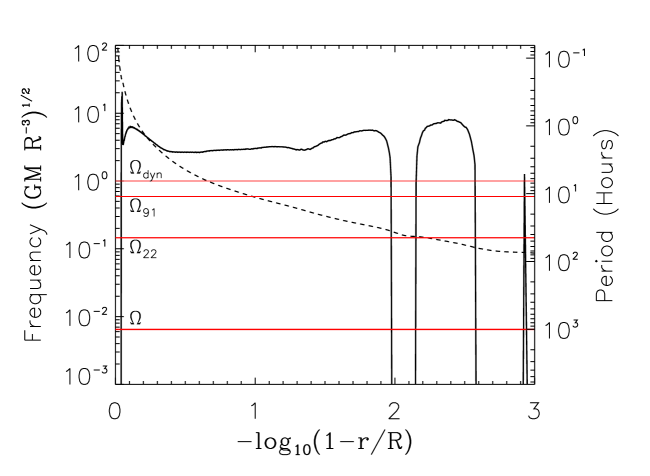
Figure 1: Propagation diagram for our $M=2.35M_{\odot}$, $R=2.34R_{\odot}$ stellar model, showing the value of $N$ (solid black line) and the Lamb frequency, $L_{2}$ (dashed black line), in units of $(GM/R^{3})^{1/2}$. The horizontal red lines denote important angular frequencies for the KOI-54 system, including (from top) the dynamical frequency of the star, $(GM/R^{3})^{1/2}$; the highest frequency mode observed in KOI-54 ($\sigma_{\alpha}=91\Omega$); the lowest frequency mode observed ($\sigma_{\alpha}=22.42\Omega$); and the orbital angular frequency, $\Omega$. The $y-$axis on the right-hand side displays the corresponding periods, in units of hours.

We use equation (14) to compute the non-resonant mode energy $E_{\alpha}\sim\Delta E_{\alpha}$. The corresponding surface displacement $\xi_{\alpha}(R)$ is then obtained from

$$|{\mbox{\boldmath$\xi$}}_{\alpha}(R)|\equiv\left({E_{\alpha}\over M_{\alpha}\sigma_{\alpha}^{2}}\right)^{1/2}.$$ (17)

Figure 2 shows the energy $\Delta E_{\alpha}$ and surface amplitude of the radial component of the displacement, ${\xi_{r}}_{\alpha}(R)$, of tidally excited modes away from resonances for the KOI-54 parameters. The radial displacement is directly related to the flux variation due to the oscillation mode (see Section 4). The most energetic modes have frequencies $80\Omega\mathrel{\raise 1.29167pt\hbox{$<$}\mkern-14.0mu\lower 2.58334pt\hbox{$\sim$}}\sigma_{\alpha}\mathrel{\raise 1.29167pt\hbox{$<$}\mkern-14.0mu\lower 2.58334pt\hbox{$\sim$}}140\Omega$, where $\Omega$ is the orbital angular frequency, depending on the stellar spin rate and the value of $m$. Low-order (high frequency) modes have larger values of $Q_{\alpha}$ but have smaller values of $K_{lm}(\sigma_{\alpha})$, so medium-order ($n\approx 15$) modes have the largest values of $\Delta E_{\alpha}$.

Figure 2: Non-resonant mode energy $\Delta E_{\alpha}$ (top), amplitude of the radial surface displacement ${\xi_{r}}_{\alpha}(R)$ (middle), and mode damping rates $\gamma_{\alpha}P$ (bottom) as a function of mode frequency $\sigma_{\alpha}$ (in units of the orbital frequency $\Omega$). The $l=m=2$ modes are plotted as open circles for $\Omega_{s}=0$ and filled circles for $\Omega_{s}=16.5\Omega$, while $m=0$ modes are plotted as triangles. The middle panel also displays the magnitude of the surface displacement, $|{\mbox{\boldmath$\xi$}}_{\alpha}(R)|$, for the $l=m=2$ modes with $\Omega_{s}=0$ (open circles connected by lines). The highest frequency modes shown are the $g_{9}$ mode for the $m=0$ and non-spinning $m=2$ cases, and the $g_{12}$ mode for the spinning $m=2$ case. The mode energy is in units of $GM^{2}/R$ and the displacement is in units of $R$.

Figure 2 also shows the magnitude of the displacement $|{\mbox{\boldmath$\xi$}}_{\alpha}(R)|$ for $m=2$ modes in the zero spin limit. The total displacement is much larger than the radial displacement for low-frequency modes because these modes are characterized by large horizontal displacements and are concentrated near the surface. Consequently, these modes have lower mode mass and the maximum of $|{\mbox{\boldmath$\xi$}}_{\alpha}(R)|$ shifts to lower frequencies compared to the maximum of $\Delta E_{\alpha}$.

The rotation rates of the KOI-54 stars are unknown. Spectroscopic observations constrain $V_{\rm rot}\sin i_{s}\mathrel{\raise 1.29167pt\hbox{$<$}\mkern-14.0mu\lower 2.58334pt\hbox{$\sim$}}10$ km s^-1, corresponding to $V_{\rm rot}\mathrel{\raise 1.29167pt\hbox{$<$}\mkern-14.0mu\lower 2.58334pt\hbox{$\sim$}}100$ km s^-1 if the spin inclination angle $i_{s}$ equals $i_{s}=5.5^{\circ}$ (Welsh et al. 2011). This implies that the spin period $P_{s}\mathrel{\raise 1.29167pt\hbox{$>$}\mkern-14.0mu\lower 2.58334pt\hbox{$\sim$}}1.2$ days and that $\Omega_{s}\mathrel{\raise 1.29167pt\hbox{$<$}\mkern-14.0mu\lower 2.58334pt\hbox{$\sim$}}30\Omega$. Although the classical equilibrium tide theory (e.g., Hut 1981) is not expected to be valid for our system (Lai 1997), we can adopt the pseudosynchronous rotation frequency $\Omega_{s}=\Omega_{\rm ps}=16.5\Omega$ [corresponding to $f_{ps}=1/(2.53~{}{\rm days})$] as a fiducial value.

To account for the effect of stellar rotation on the tidally excited modes, we adopt the perturbative approximation, valid when $\Omega_{s}$ is less than $\omega_{\alpha}^{(0)}$ (the mode frequency in the zero-rotation limit). The mode wave functions and $Q_{\alpha}$ are unchanged by the stellar rotation, while the mode frequencies are modified according to $\omega_{\alpha}=\omega_{\alpha}^{(0)}-mC_{nl}\Omega_{s}$ and $\sigma_{\alpha}=\omega_{\alpha}^{(0)}+m(1-C_{nl})\Omega_{s}$, where $C_{nl}>0$ is a constant (e.g. Unno et al. 1989) — our calculation gives $C_{nl}\simeq 0.16$ for all relevant modes. Note that in this approximation, $\varepsilon_{\alpha}=\omega_{\alpha}^{(0)}$. More accurate results can be obtained using the method of Lai (1997).

Stellar rotation increases the inertial-frame frequency $\sigma_{\alpha}$ of the $m>0$ modes, causing the dominant modes to have higher observed frequencies. However, rotation also shifts the tidal response to higher order g-modes with smaller values of $Q_{\alpha}$, so we expect rotation to lower the mode energies. Figure 2 confirms that finite (prograde) stellar rotation indeed shifts the dominant mode energy and surface amplitude to higher-order g-modes, giving rise to smaller $\Delta E_{\alpha}$ and ${\xi_{r}}_{\alpha}(R)$.

The somewhat erratic features of $\Delta E_{\alpha}$ and $\xi_{\alpha}$ as seen in Figure 2 for high-order (low frequency) modes are due to mode trapping effects created by the thin sub-surface convection zone in our stellar model. For these high-order modes, the tidal overlap integrals ($Q_{\alpha}$) depend on the precise shape of the mode wave function, and they can be easily affected by the detailed properties of the stellar envelope. Care must be taken in order to obtain reliable tidal overlap integrals for these high-order modes (see Fuller & Lai 2010).

The damping rate of a mode, $\gamma_{\alpha}$, can be estimated in the quasi-adiabatic limit via

$$\gamma_{\alpha}\approx\int^{r_{+}}_{r_{-}}k_{r}^{2}\chi(\xi_{r}^{2}+l(l+1)\xi_{\perp}^{2})\rho r^{2}dr,$$ (18)

where $\chi$ is the thermal diffusivity, $k_{r}^{2}\simeq l(l+1)N^{2}/(r^{2}\omega^{2})$ is the local radial wave number, and $r_{+}$ and $r_{-}$ are the boundaries of the mode’s propagation cavity. Equation (18) can be derived in the WKB limit from the quasi-adiabatic work function of a mode (Unno et al. 1989). The bottom panel of Figure 2 shows the values of $\gamma_{\alpha}$ calculated via equation (18) for the modes of our stellar model. Lower frequency g-modes have larger damping rates due to their larger wavenumbers and because they propagate closer to the surface of the star where the diffusivity is larger. Equation (18) provides an estimate for mode damping rates via radiative diffusion in the quasi-adiabatic limit; however, fully adiabatic oscillation equations must be solved for low-frequency modes for which $\gamma_{\alpha}$ is comparable to the mode frequency. Furthermore, modes may also damp via nonlinear processes (see Section 6).

4 Flux Variation due to Tidally-Forced Oscillations

In section 2, we considered the tidal response to be composed of the sum of the star’s natural oscillation modes, each having its own steady-state energy $E_{\alpha}$. This provides a simple relation between the resonant mode energy and non-resonant energy. The observed magnitude variation of KOI-54 has over 20 components with frequencies that are almost exact multiples of the orbital frequency, i.e., they have $\sigma_{\alpha}=(N+\epsilon)\Omega$ with $|\epsilon|\leq 0.01$. In this section, we examine the tidal response as a sum of oscillations at exact multiples of the orbital frequency. Each component $U_{lm}$ of the tidal potential can be decomposed as

$$U_{lm}=-\frac{GM^{\prime}W_{lm}r^{l}}{a^{l+1}}Y_{lm}(\theta,\phi_{i})\sum_{N=-\infty}^{\infty}F_{Nm}\,e^{-iN\Omega t},$$ (19)

where $F_{Nm}$ is defined by the expansion

$$\left({a\over D}\right)^{l+1}e^{-im\Phi}=\sum_{N=-\infty}^{\infty}F_{Nm}e^{-iN\Omega t}$$ (20)

and is given by

$$F_{Nm}=\frac{1}{\pi}\int^{\pi}_{0}d\Psi\frac{\cos\big{[}N\big{(}\Psi-e\sin\Psi\big{)}-m\Phi(t)\big{]}}{\big{(}1-e\cos\Psi\big{)}^{l}}.$$ (21)

Here, $a$ is the semi-major axis of the orbit, and $\Psi$ is the eccentric anomaly. Note that $F_{Nm}$ is related to $K_{lm}$ [see equation (15)] by $K_{lm}(\sigma_{\alpha}=N\Omega)=W_{lm}(1-e)^{l+1}\Omega^{-1}F_{Nm}$. Inserting equation (19) into equation (5) yields

$$\dot{c}_{\alpha}+(i\omega_{\alpha}+\gamma_{\alpha})c_{\alpha} =\frac{iGM^{\prime}W_{lm}Q_{\alpha}}{2\varepsilon_{\alpha}a^{l+1}}$$

$$\times\sum_{N=-\infty}^{\infty}F_{Nm}e^{i(m\Omega_{s}-N\Omega)t},$$ (22)

whose non-homogeneous solution is

$$c_{\alpha}(t)=\frac{GM^{\prime}W_{lm}Q_{\alpha}}{2\varepsilon_{\alpha}a^{l+1}}\sum_{N=-\infty}^{\infty}\frac{F_{Nm}e^{-i(N\Omega-m\Omega_{s})t}}{(\sigma_{\alpha}-N\Omega)-i\gamma_{\alpha}}.$$ (23)

The total tidal response is ${\mbox{\boldmath$\xi$}}({\bf r},t)=\sum_{\alpha}c_{\alpha}(t){\mbox{\boldmath$\xi$}}_{\alpha}({\bf r})$, where ${\mbox{\boldmath$\xi$}}_{\alpha}({\bf r})\propto e^{im\phi}$. When the displacements are expressed in terms of ${\bf r}_{i}=(r,\theta,\phi_{i})$ (the position vector in the inertial frame, with $\phi_{i}=\phi+m\Omega_{s}t$), we have

$${\mbox{\boldmath$\xi$}}({\bf r}_{i},t) =\sum_{N=-\infty}^{\infty}\sum_{\alpha}\frac{GM^{\prime}W_{lm}Q_{\alpha}}{2\varepsilon_{\alpha}a^{l+1}}\frac{F_{Nm}{\mbox{\boldmath$\xi$}}_{\alpha}({\bf r}_{i})}{(\sigma_{\alpha}-N\Omega)-i\gamma_{\alpha}}e^{-iN\Omega t}$$

$$=\sum_{N=1}^{\infty}\sum_{\alpha^{\prime}}\frac{GM^{\prime}W_{lm}Q_{\alpha}}{2\varepsilon_{\alpha}a^{l+1}}{\mbox{\boldmath$\xi$}}_{\alpha}({\bf r}_{i})$$

$$\!\!\!\!\!\!\!\!\!\!\!\times\bigg{[}\frac{F_{Nm}e^{-iN\Omega t}}{(\sigma_{\alpha}-N\Omega)-i\gamma_{\alpha}}+\frac{F_{-Nm}e^{iN\Omega t}}{(\sigma_{\alpha}+N\Omega)-i\gamma_{\alpha}}\bigg{]}+c.c.$$ (24)

where $c.c.$ denotes the complex conjugate, and $\sum_{\alpha^{\prime}}$ implies that the sum is restricted to modes with $\omega_{\alpha}>0$ (including both $m>0$ and $m<0$ modes) (by contrast, $\sum_{\alpha}$ includes both $\omega_{\alpha}>0$ and $\omega_{\alpha}<0$ terms, as well as both $m>0$ and $m<0$). We have omitted the $N=0$ term for simplicity because it is not part of the dynamical response. Each ${\mbox{\boldmath$\xi$}}_{N}$ (oscillating at frequency $N\Omega$) is then a sum over the star’s oscillation modes, with large contributions coming from nearly-resonant modes with $\sigma_{\alpha}\approx N\Omega$.

We use the result of Buta & Smith (1979) (see also Robinson et al. 1982) to estimate the magnitude variation $(\Delta\rm{mag})$ associated with each component of the tidal response. The magnitude variation of the star has two primary components: a geometrical component, $(\Delta{\rm mag})_{G}$, due to distortions in the shape of the star, and a temperature component, $(\Delta{\rm mag})_{T}$, due to perturbations in the surface temperature of the star’s photosphere.

For an $l=m=2$ mode with surface radial displacement $\xi_{r\alpha}(R)$, the amplitudes of the bolometric magnitude variations are

$$(\Delta{\rm mag})_{\alpha T}^{(m=2)} \simeq-1.7\,\gamma_{l}\sin^{2}i_{s}\,\frac{\Gamma_{2}-1}{\Gamma_{2}}$$

$$\times\bigg{[}\frac{l(l+1)}{\hat{\omega}_{\alpha}^{2}}-4-\hat{\omega}_{\alpha}^{2}\bigg{]}\frac{{\xi_{r}}_{\alpha}(R)}{R}$$ (25)

and

$$(\Delta{\rm mag})_{\alpha G}^{(m=2)}\simeq-0.42\,(\alpha_{l}+\beta_{l})\sin^{2}i_{s}\,\frac{{\xi_{r}}_{\alpha}(R)}{R}.$$ (26)

Here, $\Gamma_{2}\simeq 5/3$ is the adiabatic index of gas at the surface of the star, $\hat{\omega}=\omega_{\alpha}/\sqrt{GM/R^{3}}$ is the dimensionless mode frequency, and $\gamma_{l}\approx 0.3$ and $\alpha_{l}+\beta_{l}\approx-1.2$ are bolometric limb darkening coefficients appropriate for A stars. For KOI-54, the value of the spin inclination angle $i_{s}$ (the angle between the spin axis and the line of sight) is unknown, but we may use the system’s orbital inclination of $i_{\rm orb}=5.5^{\circ}$ as a first guess, although it is possible that the star’s spin axis is inclined relative to the orbital angular momentum axis. Similarly, for $l=2$, $m=0$ modes, the amplitudes of the magnitude variations are

$$(\Delta{\rm mag})_{\alpha T}^{(m=0)} \simeq-1.4\gamma_{l}\,\big{(}3\cos^{2}i_{s}-1\big{)}\,\frac{\Gamma_{2}-1}{\Gamma_{2}}$$

$$\times\bigg{[}\frac{l(l+1)}{\hat{\omega}_{\alpha}^{2}}-4-\hat{\omega}_{\alpha}^{2}\bigg{]}\frac{{\xi_{r}}_{\alpha}(R)}{R}$$ (27)

and

$$(\Delta{\rm mag})_{\alpha G}^{(m=0)}\simeq-0.34\,(\alpha_{l}+\beta_{l})\big{(}3\cos^{2}i_{s}-1\big{)}\frac{{\xi_{r}}_{\alpha}(R)}{R}.$$ (28)

In equations (4) and (4), the factor of $[l(l+1)/\hat{\omega}_{\alpha}^{2}-4-\hat{\omega}_{\alpha}^{2}]$ arises from the outer boundary condition formulated by Baker & Kippenhahn (1965) (see also Dziembowski 1971), in which the radial derivative of the Lagrangian pressure perturbation vanishes at the outer boundary (in our case, the stellar photosphere), such that the mode energy vanishes at infinity in an isothermal atmosphere. It is not clear how well this boundary condition applies for a real star, nor how it should be modified when non-adiabatic effects are taken into account. For the $g$-modes considered here, the factor $l(l+1)/\hat{\omega}_{\alpha}^{2}\gg 1$, causing the temperature effect to overwhelm the geometrical effect for magnitude variations.

The magnitude variation for each frequency $N\Omega$ is a sum of the variations due to individual modes:

$$(\Delta{\rm mag})_{N}=\sum_{\alpha^{\prime}}\frac{GM^{\prime}W_{lm}Q_{\alpha}a_{\alpha}}{2\varepsilon_{\alpha}a^{l+1}}\frac{{\xi_{r}}_{\alpha}(R)}{R}$$

$$\times\bigg{[}\frac{F_{Nm}e^{-iN\Omega t}}{(\sigma_{\alpha}-N\Omega)-i\gamma_{\alpha}}+\frac{F_{-Nm}e^{iN\Omega t}}{(\sigma_{\alpha}+N\Omega)-i\gamma_{\alpha}}\bigg{]}+c.c.,$$ (29)

where $a_{\alpha}$ is the constant in front of ${\xi_{r}}_{\alpha}(R)/R$ in equations (4)-(28), and $N>0$.

Using the values of $\varepsilon_{\alpha}$, $Q_{\alpha}$, ${\mbox{\boldmath$\xi$}}_{\alpha}(r)$, and $\gamma_{\alpha}$ calculated in Section 2, we compute each term $(\Delta{\rm mag})_{N}$ in equation (4). Figure 3 shows a plot of the magnitude variation as a function of $N$, along with the observed magnitude variations in KOI-54 as determined by Welsh et al. (2011). To make this plot, we have subtracted out the contribution from the “equilibrium tide”, because the equilibrium tide is responsible for the periodic brightening of KOI-54 near periastron and was subtracted out by Welsh et al. (2011) in order to obtain the magnitude variations due to tidally-induced stellar oscillations. The equilibrium tide can be computed by taking the limit $\sigma_{\alpha}\gg N\Omega$, i.e., by setting $N\Omega=0$ for each term inside the sum in equation (4). We adopt a spin inclination angle $i_{s}=10^{\circ}$.

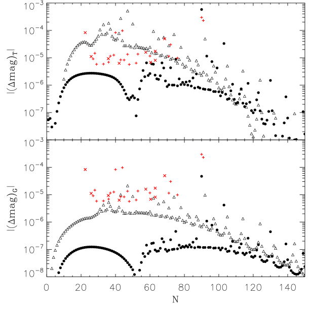
Figure 3: Magnitude variation $\Delta{\rm mag}_{N}$ as a function of $N$ due to the temperature effect (top) and geometrical effect (bottom) for $l=m=2$ modes (filled circles) and $l=2$, $m=0$ modes (triangles). We also plot the observed magnitude variations that are an integer multiple of the orbital frequency (red plus symbols), and those that are not an integer multiple of the orbital frequency (red x symbols). The plot uses $i_{s}=10^{\circ}$ and $\Omega_{s}\simeq 15\Omega$.

Figure 3 includes the magnitude variations due to the temperature effect and those due to geometrical effects. For the adopted spin inclination ($10^{\circ}$), the $m=0$ modes dominate the observed magnitude variations, although a nearly-resonant $m=2$ mode can be visible. However, it is obvious from Figure 3 that our computed variations due to the temperature effect of $m=0$ modes are appreciably larger than those observed. In fact, the magnitude variations due to geometrical effects reproduce the observed variations much more accurately. The over-prediction of the magnitude variations from the temperature effect is mostly likely due to non-adiabatic effects in the stellar atmosphere, which renders equations (4) and (4) inaccurate for low-frequency modes. Indeed, Buta & Smith (1979) also found that for main sequence B stars, the predicted magnitude variations due to the temperature effect for low-frequency modes were much larger than what was observed, and they speculated that the mismatch was due to non-adiabatic effects in the outer layers of the star.

Our results depicted in Figure 3 suggest that most of the observed magnitude variations (with the exception the highest-frequency modes) in KOI-54 are due the geometrical surface distortions produced by $m=0$ modes that happen to be nearly resonant with a harmonic of the orbital frequency. The actual magnitude variations due to the temperature effect (when non-adiabatic effects are properly taken into account near the stellar photosphere) should not be much larger than the geometric effect. Note that in Figure 3 we have plotted the absolute values of the magnitude variations for the temperature and geometrical effects, but that the temperature and geometrical effects have opposite sign and tend to cancel each other out.

To produce the highest-frequency modes ($90f_{\rm orb}$ and $91f_{\rm orb}$) observed in KIO-54, in Figure 3 we have fine-tuned the spin of the star to $\Omega_{s}\simeq 15\Omega$ such that the $N=90$ oscillation is nearly resonant with one of the star’s oscillation modes. In section 5 we argue that the $N=90$ and $N=91$ oscillations are likely due to an $m=2$ mode in each star that is locked in resonance. The fine-tuning produces a magnitude variation due to the temperature effect that is comparable to one of the observed oscillations, although the predicted geometrical magnitude variation is somewhat less than what is observed. If the $N=90$ and $N=91$ oscillations are indeed due to resonant $m=2$ modes, then it is likely that the predicted magnitude variation due to the temperature effect (based on adiabatic approximation) is more accurate for these modes due to their higher frequencies. This is not unreasonable since non-adiabatic effects in the stellar photosphere are expected to be less important for low-order (high frequency) modes, a point also emphasized by Buta & Smith (1979). In any case, a more in-depth analysis of the non-adiabatic oscillation modes (particularly their flux variations) for the stars of the KOI-54 system is needed.

5 Secular Spin-Orbit Evolution and Resonance Locking

In the previous sections we proposed that a resonance with $\sigma_{\alpha}\sim 90\Omega$ creates the largest observed magnitude variations in KOI-54. Here we study the secular evolution of the stellar spin and binary orbit, and how resonances may naturally arise during the evolution. Several aspects of tidal resonance locking in massive-star binaries were previously explored by Witte & Savonije (1999, 2001).

Dynamical tides lead to spin and orbital evolution, with the orbital energy and angular momentum evolving according to

$$\dot{E}_{\rm orb}=-\sum_{\alpha}2\gamma_{\alpha}E_{\alpha},\quad\dot{J}_{\rm orb}=-\sum_{\alpha}2\gamma_{\alpha}E_{\alpha}\frac{m}{\sigma_{\alpha}},$$ (30)

where we have used the fact that the mode angular momentum (in the inertial frame) is related to the mode energy by $J_{\alpha}=(m/\sigma_{\alpha})E_{\alpha}$. The orbital frequency $\Omega$ therefore evolves as

$$\frac{\dot{\Omega}}{\Omega}=\sum_{\alpha}\frac{f_{\alpha}}{t_{d\alpha}},$$ (31)

where

$$f_{\alpha}=\left[4\sin^{2}(\pi\sigma_{\alpha}/\Omega)+(\gamma_{\alpha}P)^{2}\right]^{-1},$$ (32)

and $t_{d\alpha}^{-1}$ specifies the orbital decay rate due to a single non-resonant mode $\alpha$:

$$t_{d\alpha}^{-1} =\frac{3\gamma_{\alpha}\Delta E_{\alpha}}{|E_{\rm orb}|}$$

$$=\frac{12\pi^{2}\gamma_{\alpha}}{(1-e)^{6}}\left(\frac{M^{\prime}}{M}\right)\left(\frac{R}{a}\right)^{5}\left(\frac{\sigma_{\alpha}}{\varepsilon_{\alpha}}\right)|Q_{\alpha}K_{lm}|^{2}.$$ (33)

Using the KOI-54 parameters and assuming $\sigma_{\alpha}\sim\varepsilon_{\alpha}$, we have

$$t_{d\alpha}^{-1}\simeq 8.9\times 10^{-10}\gamma_{\alpha}\left(\frac{Q_{\alpha}K_{lm}}{10^{-4}}\right)^{2}.$$ (34)

Resonance occurs when a mode has frequency $\sigma_{\alpha}=N\Omega$ for an integer value of $N$.

5.1 Need for Resonance Locking

We first consider how likely it is to observe a mode near resonance when $\sigma_{\alpha}$ is held constant (i.e., it does not change during the period of resonance-crossing).

As can be seen from Figure 2, the $m=2$ modes dominate tidal energy transfer in the KOI-54 system, yet (as evidenced from Figure 3), most of the visible modes (except $N=90,91$) are $m=0$ modes. Consider a particular $m=0$ mode near resonance, with $\sigma_{\alpha}=(N+\epsilon)\Omega$ and $|\epsilon|\ll 1$. Since the mode contributes little to the tidal energy transfer, the probability of being close to resonance ($|\epsilon|<\epsilon_{0}$) is simply $P_{\rm res}\simeq 2\epsilon_{0}$. Figure 3 indicates that an $m=0$ mode with $25\mathrel{\raise 1.29167pt\hbox{$<$}\mkern-14.0mu\lower 2.58334pt\hbox{$\sim$}}N\mathrel{\raise 1.29167pt\hbox{$<$}\mkern-14.0mu\lower 2.58334pt\hbox{$\sim$}}80$ requires $|\epsilon_{0}|\mathrel{\raise 1.29167pt\hbox{$<$}\mkern-14.0mu\lower 2.58334pt\hbox{$\sim$}}0.1$ to be visible [mode visibility scales as $|(\Delta{\rm mag})|\propto 1/|\epsilon|$]. In each star there are about forty $m=0$ modes in this frequency range, thus we should expect about 8 of these modes from each star to be visible, in rough agreement with Figure 3 and the observations.

Now let us consider modes that significantly influence the tidal energy transfer (these include $m=2$ modes such as the $N=90,91$ modes, but may also include $m=0$ modes very near resonance – if they occur). For the KOI-54 system, the modes that contribute significantly to the tidal energy transfer have $\sigma_{\alpha}\mathrel{\raise 1.29167pt\hbox{$>$}\mkern-14.0mu\lower 2.58334pt\hbox{$\sim$}}2\Omega_{p}\simeq 40\Omega$, thus $N=\sigma_{\alpha}/\Omega\mathrel{\raise 1.29167pt\hbox{$>$}\mkern-14.0mu\lower 2.58334pt\hbox{$\sim$}}40$. Consider a particular mode near resonance, and suppose that the tidal energy transfer is dominated by the resonant mode ($\alpha$). The orbital decay rate during the resonance is given by $\dot{P}/P=-t_{d\alpha}^{-1}\left[(2\pi\epsilon)^{2}+(\gamma_{\alpha}P)^{2}\right]^{-1}$. Thus the time that the system spends “in resonance” ($|\epsilon|<\epsilon_{0}$) is $(\Delta t)_{\epsilon_{0}}=t_{d\alpha}(2\epsilon_{0}/N)\left[(2\pi\epsilon_{0})^{2}/3+(\gamma_{\alpha}P)^{2}\right]\sim 8\pi^{2}t_{d\alpha}|\epsilon_{0}|^{3}/(3N)$. By contrast, the time it takes the orbit to evolve between resonances (for the same mode) is $(\Delta t)_{\rm nr}\sim t_{d}/N$, where $t_{d}$ is the orbital decay timescale due to all non-resonant modes ($t_{d}$ may be a factor of $\sim 10$ smaller than $t_{d\alpha}$). The probability of seeing a mode very near resonance is thus

$$P_{\rm res}=\frac{(\Delta t)_{\epsilon_{0}}}{(\Delta t)_{\rm nr}}\simeq\frac{8\pi^{2}}{3}\frac{t_{d\alpha}}{t_{d}}|\epsilon_{0}|^{3}.$$ (35)

Figure 3 indicates that (for in inclination of $i_{s}=10^{\circ}$) we require $|\epsilon_{0}|\mathrel{\raise 1.29167pt\hbox{$<$}\mkern-14.0mu\lower 2.58334pt\hbox{$\sim$}}10^{-2}$ for an $m=2$ mode to be visible, for which the probability is $P_{\rm res}\mathrel{\raise 1.29167pt\hbox{$<$}\mkern-14.0mu\lower 2.58334pt\hbox{$\sim$}}3\times 10^{-4}$. Thus, at first glance, the chances of observing even a single tidally-excited $m=2$ mode in the KOI-54 system are slim. The $N=90,91$ modes require $|\epsilon_{0}|\mathrel{\raise 1.29167pt\hbox{$<$}\mkern-14.0mu\lower 2.58334pt\hbox{$\sim$}}10^{-2}$, even if they are produced by $m=0$ modes. It is therefore extremely unlikely to observe the system with such large amplitude modes, unless (by some mechanism) they are locked into resonance. In the sections that follow, we outline such a resonance locking mechanism and how it applies to the KOI-54 system.

5.2 Critical Resonance-Locking Mode

We now consider the possibility of resonance locking for the $m=2$ modes. Tidal angular momentum transfer to the star increases the stellar spin $\Omega_{s}$, thereby changing the mode frequency $\sigma_{\alpha}$. There exists a particular resonance, $\sigma_{\alpha}=N_{c}\Omega$, for which $\sigma_{\alpha}$ and $\Omega$ change at the same rate, i.e.,

$${\dot{\sigma}_{\alpha}\over\sigma_{\alpha}}={\dot{\Omega}\over\Omega},$$ (36)

so that the resonance can be maintained once it is reached. With $\dot{J}_{s}=-\dot{J}_{\rm orb}$ and the mean stellar rotation rate $\bar{\Omega}_{s}=J_{s}/I$ (where $I$ is the moment of inertia), we have $\dot{\sigma}_{\alpha}=mB_{\alpha}\dot{J}_{s}/I$, where $B_{\alpha}\equiv(d\sigma_{\alpha}/d\bar{\Omega}_{s})/m$. Assuming that a single resonant mode dominates the tidal energy and angular momentum transfer, we find $\dot{\sigma}_{\alpha}/\sigma_{\alpha}=-m^{2}B_{\alpha}\dot{E}_{\rm orb}/(IN^{2}\Omega^{2})$. Thus

$$\left({\dot{\sigma}_{\alpha}\over\sigma_{\alpha}}\right)_{\rm tide}=\left(\frac{N_{c}}{N}\right)^{2}\left({\dot{\Omega}\over\Omega}\right)_{\rm tide},$$ (37)

where

$$N_{c}=m\left(\frac{B_{\alpha}\mu a^{2}}{3I}\right)^{1/2}$$ (38)

(with $\mu=MM^{\prime}/M_{t}$ the reduced mass of the binary) corresponds to the critical resonance-locking mode. The subscript “tide” in equation (37) serves as a reminder that the changes of $\sigma_{\alpha}$ and $\Omega$ are due to the tidal interaction.

For the KOI-54 parameters (with $a\simeq 39R$ and $m=2$), we have

$$N_{c}\simeq 131\left({B_{\alpha}\over 0.84}\right)^{1/2}\left({\kappa\over 0.05}\right)^{-1/2},$$ (39)

where $\kappa=I/(MR^{2})$. If we assume that the star maintains rigid-body rotation during tidal spin up, then $B_{\alpha}=1-C_{nl}$. Numerical calculation for our stellar model gives $B_{\alpha}\simeq 0.84$ (with very weak dependence on modes) and $\kappa\simeq 0.040$, giving $N_{c}\simeq 146$; a less evolved star would have $\kappa\simeq 0.047$, giving $N_{c}\simeq 135$. Note that in the above we consider only tides in one star ($M$) – when tides in the other star are considered, $\dot{\Omega}$ would be larger and the effective value of $N_{c}$ would be reduced. If identical resonances occur in the two stars, the effective value of $N_{c}$ would be reduced by a factor of $\sqrt{2}$ to $N_{c}\simeq 92$ (for $\kappa=0.05$). See section 5.3.3 and equations (70)-(71) below.

The above consideration assumes that the spin evolution of the star is entirely driven by tide. In reality, the star can experience intrinsic spindown, either due to a magnetic wind or due to radius expansion associated with stellar evolution. We may write $\dot{\Omega}_{s}=(\dot{\Omega}_{s})_{\rm tide}-|\dot{\Omega}_{s}|_{\rm sd}$, where the second term denotes the contribution due to the intrinsic spindown. The corresponding rate of change for $\sigma_{\alpha}$ is then

$${\dot{\sigma}_{\alpha}\over\sigma_{\alpha}}=\left({\dot{\sigma}_{\alpha}\over\sigma_{\alpha}}\right)_{\rm tide}-\left|{\dot{\sigma}_{\alpha}\over\sigma_{\alpha}}\right|_{\rm sd}.$$ (40)

On the other hand, the orbital evolution remains solely driven by tides:

$${\dot{\Omega}\over\Omega}=\left({\dot{\Omega}\over\Omega}\right)_{\rm tide}=\left(\frac{N}{N_{c}}\right)^{2}\left({\dot{\sigma}_{\alpha}\over\sigma_{\alpha}}\right)_{\rm tide}.$$ (41)

Comparing equations (40) and (41), we see that $N_{c}$ represents the upper boundary for resonance locking: for $N>N_{c}$, resonance locking ($\dot{\sigma}_{\alpha}/\sigma_{\alpha}=\dot{\Omega}/\Omega$) is not possible. For $N<N_{c}$, resonance locking can be achieved: the value of $(\dot{\sigma}_{\alpha}/\sigma_{\alpha})_{\rm tide}$ depends on the closeness to the resonance, which in turn depends on the intrinsic spindown timescale of the star [see equations (54) and (55) below].

The fact that $N_{c}$ naturally falls in the range close to $N=90$ and $N=91$, the most prominent modes observed in KOI-54, is encouraging. In the next subsection, we consider how the system may naturally evolve into a resonance-locking state with $N<N_{c}$.

5.3 Evolution Toward Resonance

As noted above, even in the absence of tides, the star can experience spin-down, either due to magnetic wind or due to radius expansion associated with stellar evolution. Furthermore, the intrinsic mode frequencies will change as the internal structure of the star changes due to stellar evolution. We now show that these effects can naturally lead to evolution of the system toward resonance locking.

The evolution equation for the stellar spin reads $\dot{\Omega}_{s}=-(\dot{J}_{\rm orb}/I)-(\Omega_{s}/t_{\rm sd})$, where $t_{\rm sd}$ is the “intrinsic” stellar spin-down time scale associated with radius expansion and/or magnetic braking. Using equation (30), we have

$${\dot{\Omega}_{s}\over\Omega_{s}}=\sum_{\alpha}\left({m\mu a^{2}\over 3I}\right)\left({\Omega^{2}\over\Omega_{s}\sigma_{\alpha}}\right){f_{\alpha}\over t_{d\alpha}}-{1\over t_{\rm sd}}.$$ (42)

From equation (30), we find that the orbital frequency and eccentricity evolve according to

$${\dot{\Omega}\over\Omega}=\sum_{\alpha}{f_{\alpha}\over t_{d\alpha}},$$ (43)

$${e\,{\dot{e}}\over 1-e^{2}}=-{1\over 3}\sum_{\alpha}{f_{\alpha}\over t_{d\alpha}}\left[1-{m\Omega\over\sigma_{\alpha}(1-e^{2})^{1/2}}\right].$$ (44)

To leading order in $\Omega_{s}$, the mode frequency depends on $\Omega_{s}$ via

$$\sigma_{\alpha}=\omega_{\alpha}^{(0)}+mB_{\alpha}\Omega_{s}.$$ (45)

For simplicity, we assume that the secular change of $\sigma_{\alpha}$ is only caused by the $\Omega_{s}$-evolution (e.g., we neglect the variation of $\omega_{\alpha}^{(0)}$ due to stellar evolution – this effect can be absorbed into the spindown effect on the mode; see Witte & Savonije 1999).

5.3.1 Single Mode Analysis

To gain some insight into the evolutionary behavior of the system, we first consider the case where one of the modes is very close to resonance, i.e.,

$$\sigma_{\alpha}=(N+\epsilon)\Omega,$$ (46)

while all the other modes are non-resonant. We then write the orbital and spin frequency evolution equations as

$${\dot{\Omega}\over\Omega}={f_{\alpha}\over t_{d\alpha}}+{1\over t_{d}},$$ (47)

$${\dot{\Omega}_{s}\over\Omega_{s}}={N_{c}^{2}\over mB_{\alpha}}{\Omega^{2}\over\Omega_{s}\sigma_{\alpha}}{f_{\alpha}\over t_{d\alpha}}-{1\over t_{sd}}+{1\over t_{su}}.$$ (48)

Here $t_{d}^{-1}$ and $t_{su}^{-1}$ are the orbital decay rate and spin up rate due to all the non-resonant modes. They are approximately given by

$$t_{d}^{-1}\simeq\sum_{\alpha}3\gamma_{\alpha}{\Delta E_{\alpha}\over|E_{\rm orb}|}\sim{3\gamma\Delta E\over|E_{\rm orb}|},$$ (49)

$$t_{su}^{-1}\simeq{1\over I\Omega_{s}}\sum_{\alpha}2\gamma_{\alpha}{m\over\sigma_{\alpha}}\Delta E_{\alpha}\sim{2\gamma\Delta J\over I\Omega_{s}},$$ (50)

where $\Delta E=\sum_{\alpha}\Delta E_{\alpha}$ and $\Delta J=\sum_{\alpha}(m/\sigma_{\alpha})\Delta E_{\alpha}$ are the energy and angular momentum transferred from the orbit to the star in the “first” periastron passage (see Section 2), and $\gamma$ is the characteristic mode damping rate of the most important modes in the energy transfer. Since $\Delta J\sim\Delta E/\Omega_{p}$ (where $\Omega_{p}$ is the orbital frequency at periastron), we find

$${t_{su}^{-1}\over t_{d}^{-1}}\sim{\mu a^{2}\over 3I}{\Omega^{2}\over\Omega_{s}\Omega_{p}}.$$ (51)

Note that $t_{d}^{-1}$ can be a factor of a few ($\sim 10$) larger than $t_{d\alpha}^{-1}$, and $t_{su}^{-1}$ is a factor of a few larger than $t_{d}^{-1}$.

Equations (46)-(48) can be combined to yield the evolution equation for $\epsilon=\sigma_{\alpha}/\Omega-N$:

$${\dot{\epsilon}\over N}=\left[\left({N_{c}\over N}\right)^{2}-1\right]{f_{\alpha}\over t_{d\alpha}}-{1\over t_{D}},$$ (52)

where

$${1\over t_{D}}={mB_{\alpha}\Omega_{s}\over N\Omega}\left({1\over t_{sd}}-{1\over t_{su}}\right)+{1\over t_{d}}.$$ (53)

Equation (52) provides the key for understanding the condition of achieving mode locking:

(i) For $N>N_{c}$: The RHS of Equation (52) is always negative, and the system will pass through the resonance ($\epsilon=0$) without locking. Physically, the reason is that for $N>N_{c}$, the orbit decays faster (during resonance) than the mode frequency can catch up, so the system sweeps through the resonance.

(ii) For $N<N_{c}$ and $t_{D}^{-1}\gg t_{d\alpha}^{-1}$: Starting from a non-resonance initial condition ($\epsilon_{\rm in}\sim 0.5$, or $f_{\alpha}\sim 1$), the system will evolve toward a resonance-locking state ($\dot{\epsilon}=0$), at which

$$f_{\alpha}={t_{d\alpha}\over\delta_{N}t_{D}}\gg 1$$ (54)

where $\delta_{N}\equiv(N_{c}/N)^{2}-1$. The “equilibrium” value of $\epsilon$ is given by

$$\epsilon_{\rm eq}\simeq{1\over 2\pi}\left[{t_{D}\delta_{N}\over t_{d\alpha}}-(\gamma_{\alpha}P)^{2}\right]^{1/2}\ll 1.$$ (55)

This resonance-locking state can be achieved when

$$t_{D}\delta_{N}/t_{d\alpha}>(\gamma_{\alpha}P)^{2},$$ (56)

as otherwise resonance “saturation” [$f_{\alpha}\leq(\gamma_{\alpha}P)^{-2}$] occurs, and the system will sweep through the resonance. Note that during the resonance-locking phase, the stellar spin increases as

$${\dot{\Omega}_{s}\over\Omega_{s}}={1\over\delta_{N}}\left(t_{sd}^{-1}-t_{su}^{-1}\right)+{N_{c}^{2}\Omega\over N\delta_{N}mB_{\alpha}\Omega_{s}}t_{d}^{-1},$$ (57)

and the orbital frequency increases as

$$\frac{\dot{\Omega}}{\Omega}=\frac{mB_{\alpha}}{N\delta_{N}}\frac{\Omega_{s}}{\Omega}\Big{(}t_{sd}^{-1}-t_{su}^{-1}\Big{)}+\frac{N_{c}^{2}}{N^{2}\delta_{N}}t_{d}^{-1}.$$ (58)

The above analysis assumes $t_{D}^{-1}>0$. In the absence of the intrinsic stellar spin-down (i.e., $t_{sd}^{-1}=0$), we have

$$t_{D}^{-1}\sim-{N_{c}^{2}\over mN}\left({20\Omega\over\Omega_{p}}\right)t_{d}^{-1}+t_{d}^{-1}.$$ (59)

Thus $t_{D}$ can be negative for $N\mathrel{\raise 1.29167pt\hbox{$<$}\mkern-14.0mu\lower 2.58334pt\hbox{$\sim$}}N_{c}^{2}/40$. In this case, one may expect mode-locking for $N>N_{c}$. Nevertheless, $t_{D}^{-1}$ is only moderately larger (a factor of 10 or so) than $t_{d\alpha}^{-1}$ without intrinsic spin-down, so a close resonance with $f_{\alpha}\gg 1$ (or $|\epsilon|\ll 1$) is unlikely.

5.3.2 Resonance Locking for $m=0$ Modes

Above (and in other sections of this paper), we considered the frequency of a mode in the inertial frame to first order in $\Omega_{s}$: $\sigma_{\alpha}=\varepsilon_{\alpha}+mB_{\alpha}\Omega_{s}$. In this approximation, $m=0$ modes have constant frequency and thus cannot lock into resonance. However, Lai (1997) find that to second order in $\Omega_{s}$, the frequency of $m=0$ modes can be approximated by

$$\frac{\sigma_{\alpha,m=0}}{\varepsilon_{\alpha}}\simeq 1+\frac{6}{7}\bigg{(}\frac{\Omega_{s}}{\varepsilon_{\alpha}}\bigg{)}^{2}.$$ (60)

Recall that $\varepsilon_{\alpha}$ is the mode frequency in the absence of rotation. Thus, to second order, the frequency of $m=0$ modes can change and resonance locking is possible.

Let us examine the scenario in which an $m_{\alpha}=2$ mode with $N_{m=2}\simeq 90$ is locked in resonance, as we suspect is the case for KOI-54. Assuming this mode dominates the tidal interaction, the system evolves such that

$$N_{m=2}\dot{\Omega} =\dot{\sigma}_{\alpha,m=2}$$

$$=m_{\alpha}B_{\alpha}\dot{\Omega}_{s},$$ (61)

Then there will be a value of $N_{m=0}$ for an $m=0$ mode such that

$$N_{m=0}\dot{\Omega}=\dot{\sigma}_{\alpha,m=0}.$$ (62)

Using equation (5.3.2) for the LHS of equation (62), equation (60) for the RHS of equation (62), and the condition $\sigma_{\alpha,m=0}=N_{m=0}\Omega$, we find

$$N_{m=0}=\bigg{[}\frac{12N_{m=2}}{7m_{\alpha}B_{\alpha}\big{[}\Omega/\Omega_{s}-m_{\alpha}B_{\alpha}/(2N_{m=2})\big{]}}\bigg{]}^{1/2}.$$ (63)

Using $N_{m=2}=90$, $m_{\alpha}=2$, $B_{\alpha}=0.84$, and $\Omega_{s}=\Omega_{ps}=16.5\Omega$, we find that $N_{m=0}\simeq 42$. Thus, an $m=0$ mode with $\sigma_{\alpha}\simeq 42\Omega$ may be able to stay close to resonance for an extended period of time. KOI-54 has two very visible modes at $\sigma_{3}=44\Omega$ and $\sigma_{4}=40\Omega$. We speculate that these modes may correspond to an $m=0$ mode in each star that is nearly locked in resonance due to the orbital evolution produced by a locked $m=2$ mode with $N_{m=2}\simeq 90$. However, because the value of $N_{m=0}$ depends on $\Omega_{s}$ (which is currently unknown for KOI-54), we will not consider $m=0$ mode locking in the remainder of this paper.

5.3.3 Resonance Locking in Both Stars

In Section 5.3.1, we considered resonant locking of an $m=2$ mode in the primary star $M$. Since the two stars in the KOI-54 system are quite similar, resonant locking may be achieved in both stars simultaneously. We now consider the situation in which an $m=2$ mode $\sigma_{\alpha}$ in star $M$ and an $m^{\prime}=2$ mode $\sigma_{\alpha^{\prime}}$ in star $M^{\prime}$ are both very close to orbital resonance, i.e.,

$$\sigma_{\alpha}=(N+\epsilon)\Omega,\qquad\sigma_{\alpha^{\prime}}=(N^{\prime}+\epsilon^{\prime})\Omega,$$ (64)

while all other modes (in both stars) are non-resonant. Here, all primed quantities refer to star $M^{\prime}$, and unprimed quantities refer to star $M$. The orbital evolution equation then reads

$${\dot{\Omega}\over\Omega}={f_{\alpha}\over t_{d\alpha}}+{f_{\alpha^{\prime}}\over t_{d\alpha^{\prime}}}+{1\over t_{d}},$$ (65)

while the spin evolution is governed by equation (57) for star $M$ and a similar equation for $M^{\prime}$. We then find

$${\dot{\epsilon}\over N}=\left[\left({N_{c}\over N}\right)^{2}-1-x\right]{f_{\alpha}\over t_{d\alpha}}-{1\over t_{D}},$$ (66)

$${\dot{\epsilon}^{\prime}\over N^{\prime}}=\left[\left({N_{c}^{\prime}\over N^{\prime}}\right)^{2}-1-{1\over x}\right]{f_{\alpha^{\prime}}\over t_{d\alpha^{\prime}}}-{1\over t_{D}^{\prime}},$$ (67)

where

$$x\equiv{f_{\alpha^{\prime}}/t_{d\alpha^{\prime}}\over f_{\alpha}/t_{d\alpha}}={\dot{E}_{\alpha^{\prime}}\over\dot{E}_{\alpha}},$$ (68)

with $\dot{E}_{\alpha}$ and $\dot{E}_{\alpha^{\prime}}$ the energy dissipation rates (including resonances) due to the resonant modes in star $M$ and $M^{\prime}$, respectively. Thus, analogous to Section 5.3.1, for $t_{D}>0$ and $t_{D}^{\prime}>0$, the necessary conditions for resonant mode locking in both stars are

$$N<N_{c,{\rm eff}},\quad{\rm and}\quad N^{\prime}<N_{c,{\rm eff}}^{\prime},$$ (69)

with

$$N_{c,{\rm eff}}={N_{c}\over\sqrt{1+x}}=m\left[{B_{\alpha}\mu a^{2}\over 3I(1+x)}\right]^{1/2},$$ (70)

$$N_{c,{\rm eff}}^{\prime}={N_{c}^{\prime}\over\sqrt{1+x^{-1}}}=m^{\prime}\left[{B_{\alpha^{\prime}}\mu a^{2}\over 3I^{\prime}(1+x^{-1})}\right]^{1/2}.$$ (71)

Obviously, if the two stars have identical resonances ($x=1$), then $N_{c,{\rm eff}}$ would be smaller than $N_{c}$ by a factor of $\sqrt{2}$. If the energy dissipation rates in the two stars differ by at least a factor of a few (e.g., $x\sim 0.2$), then $N_{c,{\rm eff}}$ is only slightly modified from $N_{c}$, while $N_{c,{\rm eff}}^{\prime}$ will be a factor of a few smaller than $N_{c}^{\prime}$.

5.4 Numerical Examples of Evolution Toward Resonance

For a given set of modes, the solution of the system of equations (42)-(44) depends on the dimensionless parameters $t_{d\alpha}/t_{sd}$, $N_{c}$ and $\gamma_{\alpha}P$, as well as the initial conditions. In general, these parameters change as the system evolves.

5.4.1 A Simple Example

Figure 4: Secular evolution of the stellar spin and binary orbit driven by dynamical tides and “intrinsic” stellar spin-down. Two modes are included, both having $m=2$, $t_{d\alpha}/t_{sd}=100$ and $\gamma_{\alpha}P=0.01$. The initial spin frequency is $\Omega_{s}=15\Omega$. The top panel shows the orbital frequency (solid line) and the spin frequency (dashed line), both in units of their initial values. The second panel shows $N_{c}$ as defined by equation (38). The bottom two panels show the mode frequencies in units of $\Omega$. The two light dotted lines on the third panel also show $\sigma_{1}/\Omega$ and $\sigma_{2}/\Omega$. The time (on the horizontal axis) is expressed in units of $t_{sd}$, the intrinsic spindown time of the star. The system first evolves into resonance locking at $\sigma_{1}=100\Omega$ and then a different resonance locking at $\sigma_{2}=90\Omega$. Note that resonance locking cannot occur when $\sigma_{\alpha}/\Omega>N_{c}$.

To illustrate the essential behavior of the secular evolution toward resonance locking, we first consider the simple case where $t_{d\alpha}/t_{d}$ and $\gamma_{\alpha}P$ are assumed to be constant and identical for all modes considered. Figure 4 depicts an example: we include two $m=2$ modes ($\sigma_{1}$ and $\sigma_{2}$), both have $t_{d\alpha}/t_{sd}=10^{2}$, $\gamma_{\alpha}P=10^{-2}$ and $B_{\alpha}=0.8$. The parameter $N_{c}$ has an initial value of $110$, but we allow $N_{c}$ to evolve via $N_{c}\propto\Omega^{-2/3}$. At $t=0$, the spin frequency is $\Omega_{s}=15\Omega$, and the two modes have $\sigma_{1}/\Omega=100.5$ and $\sigma_{2}/\Omega=89.5$ (i.e., both are initially “off-resonance”). We see that the stellar spindown first causes $\sigma_{1}$ to lock into resonance at $\sigma_{1}/\Omega=100$. The star then spins up, driven by the resonant tidal torque. The second mode passes through the $N=90$ resonance, but it produces a negligible effect on the $\sigma_{1}/\Omega=100$ resonance. In the meantime, the orbit decays, reducing $N_{c}$. When $N_{c}$ becomes less than $100$, the resonance locking can no longer be maintained, and $\sigma_{1}$ breaks away from the $N=100$ resonance. The stellar spin then decreases (due to the $1/t_{sd}$ term), which leads to $\sigma_{2}$ to capture into the $N=90$ resonance. Eventually, as $N_{c}$ decreases (due the resonant tidal torque) below $90$, the second mode breaks away from the $N=90$ resonance. This example corroborates our analytical result of section 5.3, and demonstrates that resonance locking can indeed be achieved and maintained for an extended period during the evolution of the binary system.

5.4.2 More Realistic Examples

Having demonstrated how resonance locking can occur in a simplified system consisting of only two oscillation modes, we now investigate how resonance locking is likely to occur in the actual KOI-54 system. We solve the orbital evolution equations (42)-(45) using the actual values of $\varepsilon_{\alpha}$, $Q_{\alpha}$, and $\gamma_{\alpha}$ found in section 3 to calculate each $t_{d\alpha}$. We include eighteen modes in our equations: they are the $l=2$, $m=0$, $m=\pm 2$ modes for six values of $\varepsilon_{\alpha}$ such that the initial frequencies of the $m=2$ modes range from $40\Omega$ to $170\Omega$. We allow the value of $K_{lm}$ to evolve as the values of $\sigma_{\alpha}$, $\Omega$, and $e$ change with time.

Figures 5 and 6 display the evolution of $\Omega$, $\Omega_{s}$, $N_{c}$, and the values of $\sigma_{\alpha}$ and $E_{\alpha}$ for a selected sample of modes over a time span of tens of millions years. We use initial values of $\Omega_{o}=0.95\Omega_{\rm obs}$ (here $\Omega_{\rm obs}$ is the observed orbital frequency of KOI-54), $e_{o}=0.84$, $\Omega_{s,o}=\Omega_{ps}\simeq 16.5\Omega_{o}$, and a spindown time of $t_{sd}=3\times 10^{8}$ years. In Figure 6, we have doubled the orbital decay rate to account for an equal amount of energy dissipation in the companion star.

Let us start by examining Figure 5. The system quickly enters a resonance locking state with the $\sigma_{3,2}$ mode, where the notation $\sigma_{k,m}$ identifies the mode with the $k$th largest frequency in our simulation with azimuthal number $m$. The resonance locking lasts for over 100 million years, until the $\sigma_{2,2}$ mode reaches resonance. The $\sigma_{2,2}$ mode then locks in resonance for over 100 million years. During resonance locking, the orbital frequency and spin frequency increase rapidly. The energies $E_{\alpha}$ of the resonant locked modes can exceed $700$ their non-resonant values $\Delta E_{\alpha}$, corresponding to an increase in visibility of over 25 times the visibility during a non-resonant state. When no mode is locked in resonance, the orbital evolution is relatively slow, with the dominant effect being the spindown of the star due to the $t_{sd}$ term.

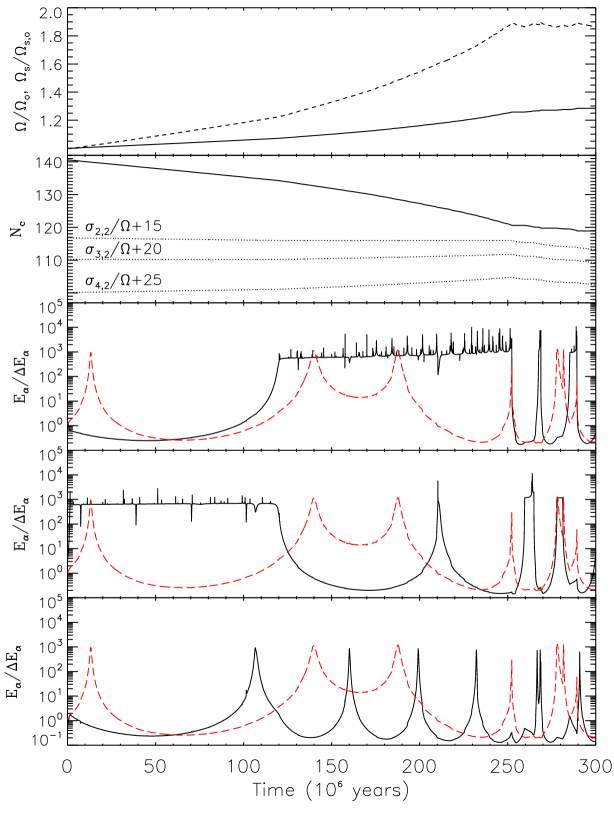
Figure 5: Secular evolution of the KOI-54 system driven by a sample of 18 oscillation modes and intrinsic stellar spindown. Top: orbital frequency $\Omega$ (solid line) and spin frequency $\Omega_{s}$ (dashed line) in units of their initial values. Top middle: the value of $N_{c}$ (solid line) and the mode frequencies $\sigma_{2,2}/\Omega+15$, $\sigma_{3,2}/\Omega+20$, and $\sigma_{4,2}/\Omega+35$ (dotted lines) of the modes depicted in the bottom three panels. Middle: the mode energy $E_{\alpha}$ in units of $\Delta E_{\alpha}$ for the $\sigma_{2,2}$ mode (solid line) and the $\sigma_{4,0}$ mode (red dashed line). Bottom middle: same as middle except the solid line is for the $\sigma_{3,2}$ mode. Bottom: same as bottom middle except the solid line is for the $\sigma_{4,2}$ mode. The initial spin frequency is $\Omega_{s}\simeq 16.5\Omega$, and the spindown time is $t_{sd}=3\times 10^{8}$ years.

For the initial conditions and orbital evolution depicted in Figure 5, only two of our 18 modes pass through resonant locking phases: two $m=2$ modes with initial frequencies of $\sigma_{2,2,o}\simeq 103$ and $\sigma_{3,2,o}\simeq 90$. The highest frequency $m=2$ mode included in our evolution does not lock in resonance because it has $N>N_{c}$ at all times. The lowest frequency modes do not lock in resonance because they do not satisfy equation (56), i.e., they become saturated before they can begin to resonantly lock. This occurs because the value of $Q_{\alpha}$ for these high-order modes is small, resulting in a small orbital decay rate $t_{d\alpha}^{-1}$ for these modes.

Which mode locks into resonance is dependent on the initial conditions. However, as can be seen in Figure 5, the resonance with the $\sigma_{2,2}$ mode ends the resonance with the $\sigma_{3,2}$ mode because the $\sigma_{2,2}$ mode has a larger value of $E_{\alpha}$ and will thus dominate the orbital decay. Therefore, we can expect the system to evolve into a state in which the mode with the largest value of $E_{\alpha}$ (and with $N<N_{c}$) is locked in resonance.

In Figure 5, the resonance locking with the $\sigma_{2,2}$ mode is ended by a resonance with the $\sigma_{4,0}$ mode. The $\sigma_{4,0}$ mode does not lock into resonance because an $m=0$ mode cannot change the stellar spin frequency. However, its resonance causes the value of $\dot{\Omega}/\Omega$ to exceed the value of $\dot{\sigma}_{\alpha}/\sigma_{\alpha}$ for the locked mode, so that the system sweeps through the resonance. In other words, the non-locked resonant mode temporarily decreases the value of $t_{d}$, decreasing the value of $t_{D}$ such that resonant saturation occurs for the locked mode, causing it to pass through resonance. Also note that even though the $\sigma_{4,0}$ mode does not lock into resonance, it maintains a relatively large energy ($E_{\alpha}>10\Delta E_{\alpha}$) for a period of over 50 million years. This is indicative of the pseudo-resonance locking for $m=0$ modes described in Section 5.3.2.

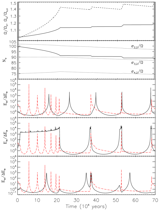
Figure 6: Same as Figure 5, except this evolution doubles the orbital decay rate due to each mode, and the red dashed line corresponds to the $\sigma_{2,0}$ mode.

Let us now examine Figure 6, in which the orbital decay rate has been doubled (i.e., we multiply $\dot{\Omega}$ by 2) to account for an equal tidal response in the companion star. The results are significantly different: due to the increased orbital decay rate, the initial effective value of $N_{c,{\rm eff}}$ has dropped to $\sim 100$ (see section 5.3.3) so that the $\sigma_{2,2}$ mode can no longer lock into resonance. Also, the maximum energy $E_{\alpha}/\Delta E_{\alpha}$ of the modes is larger in this scenario (because the modes must enter deeper into resonance to become locked), so the modes can create larger magnitude variations while being locked in resonance.

However, the resonance locking events are shorter because the modes are nearly saturated during resonance locking, allowing resonances with $m=0$ modes or higher frequency $m=2$ modes to easily disrupt the resonance locking state. In the bottom three panels of Figure 6, we have plotted the energy $E_{\alpha}$ of the $\sigma_{2,0}$ mode. In Figure 6, three of the resonant locking events for the $\sigma_{3,2}$ mode are ended due to a resonance with the $\sigma_{2,0}$ mode. We have examined the results carefully and found that all of the resonance locking events were ended due a resonance with an $m=0$ mode or an $m=2$ mode for which $N>N_{c}$. Although the resonance locking events are brief at the end of the simulation, the locking event with the $\sigma_{3,2}/\Omega=90$ mode lasts for about 20 million years at the beginning of the simulation when the system’s parameters most closely resemble those of KOI-54. We thus conclude it is likely to observe a system such as KOI-54 in a resonance locking state.

We note the secular evolution analysis presented above does not take into account the fluctuation of mode amplitudes due to the changing strength of the tidal potential in an elliptical orbit. Therefore, in addition to the results displayed above, we have also performed calculations of the full dynamic evolution of the stellar oscillations and binary orbit, including the back-reaction of the modes on the orbit. We find that resonance locking can indeed be maintained for extended periods of time, and that non-secular effects have little impact on the results discussed above.

6 Oscillations at Non-Orbital Harmonics

As discussed in section 4, in the linear theory, tidally-forced stellar oscillations give rise to flux variations at integer multiples of the orbital frequency. Many of these oscillations have been observed in the KOI-54 system. However, Welsh et al. (2011) also reported the detection of nine modes that do not have frequencies that are integer multiples of the orbital period, and their observation requires an explanation.

One possibility is that one (or both) of the stars in KOI-54 are $\delta$-Scuti variable stars. The masses, ages, and metallicities of the KOI-54 stars put them directly in the instability strip and so $\delta$-Scuti-type pulsations are not unexpected. However, as pointed out by Welsh et al. (2011), the complete absence of any modes detected with periods less than 11 hours is troublesome for the $\delta$-Scuti interpretation, as most observed $\delta$-Scuti pulsations have periods on the order of a few hours. One would then have to explain why only long period ($P>11$ hours) $\delta$-Scuti-type oscillations are visible in this system.

Another possibility is that some (or all) of the non-harmonic modes are excited via nonlinear couplings with resonant modes. In particular, it is thought that three-mode resonant coupling (parametric resonance) plays an important role in limiting the saturation amplitudes of overstable g-modes in ZZ-Ceti stars (Wu & Goldreich 2001) and $\delta$-Scuti stars (Dziembowski & Krolikowska 1985). In the KOI-54 system, when a resonantly excited mode reaches sufficiently large amplitude, it will couple to two non-resonant, lower-frequency daughter modes (see Kumar & Goodman 1996), thereby explaining the observed non-harmonic oscillations.

Parametric resonance can occur when $\omega_{\gamma}\simeq\omega_{\alpha}+\omega_{\beta}$, where $\omega_{\gamma}$ is the frequency of the parent mode and $\omega_{\alpha}$ and $\omega_{\beta}$ are the frequencies of the two daughter modes. The additional requirement that $m_{\gamma}=m_{\alpha}+m_{\beta}$, where $m$ is the azimuthal number of the mode, implies that $\sigma_{\gamma}\simeq\sigma_{\alpha}+\sigma_{\beta}$. Examination of the KOI-54 data given in Welsh et al. (2011) reveals that $f_{2}=f_{5}+f_{6}$ (25.195 $\mu$Hz = 6.207 $\mu$Hz + 18.988 $\mu$Hz) exactly to the precision of the measurements, where $f_{p}$ is the frequency of the magnitude oscillation with the $p$th largest magnitude variation. This provides strong evidence that the $p=5$ and $p=6$ oscillations are due to modes excited via parametric resonance and not via direct tidal forcing.

However, no other pair of observed non-harmonic magnitude oscillations have frequencies which add up to that of an observed oscillation. Some of these non-resonant oscillations may be due to modes excited via parametric resonance that have undetected sister modes. This possibility is especially appealing if one considers the scenario in which one of the two daughter modes has $m=0$ (and could thus be easily detected for small values of $i_{s}$), while its sibling has $m=2$ (and is thus very difficult to detect for small $i_{s}$). We therefore suggest that all non-harmonic flux oscillations are produced by nonlinear mode coupling. Deeper observations (with better photometry) and analysis may reveal additional evidence for nonlinear mode couplings in the KOI-54 system

7 Discussion

We have shown that many properties of flux oscillations detected in the KOI-54 binary system by KEPLER can be understood using the theory of dynamical tidal excitations of g-modes developed in this paper. In particular, our analysis and calculation of the resonance mode locking process, which is driven by dynamical tides and intrinsic stellar spindown, provides a natural explanation for the fact that only those modes with frequencies ($\sigma_{\alpha}$) less than about 90-100 times the orbital frequency ($\Omega$) are observed. Our result suggests that the KOI-54 system is currently in a resonance-locking state in which one of the stars has a rotation rate such that it possesses a $m=2$ mode with frequency $\sigma_{\alpha}=90\Omega$ and the other star has a similar mode with $\sigma_{\alpha^{\prime}}=91\Omega$ — these modes produce the largest flux variations detected in KOI-54. Our analysis shows that the system can evolve into and stay in such a resonance locking state for relatively long time periods, and it is reasonable to observe the system in such a state. Other less prominent flux variations at lower frequencies can be explained by the $m=0$ tidally forced oscillations, many of which may be enhanced by the resonant effect. We have also found evidence of nonlinear three-mode coupling from the published KEPLER data and suggested that the nonlinear effect may explain the flux variabilities at non-harmonic frequencies.

In our study, we have used approximate quasiadiabatic mode damping rates. Obviously, it would be useful to repeat our analysis using more realistic mode damping rates, calculated with the full non-adiabatic oscillation equations. Our calculations of the flux variations of tidally induced oscillations have also highlighted the importance of accurate treatment of non-adiabatic effects in the stellar photosphere. We have only considered g-modes (modified by stellar rotation) in this paper. Our general theory allows for other rotation-driven modes, such as inertial/Rossby modes. It would be interesting to study tidal excitations of these modes as well as the nonlinear 3-mode coupling effect in the future.

More detailed modelling of the observed oscillations may provide useful constraints on the parameters of the KOI-54 system, particularly the stellar rotation rates and spin inclinations. On a more general level, KOI-54 may serve as a “laboratory” for calibrating theory of dynamical tides, which has wide applications in stellar and planetary astrophysics (see references in Section 1).

While we believe that our current theory provides the basis for understanding many aspects of the KOI-54 observations, some puzzles remain. In our current interpretation, the most prominent oscillations (at $90\Omega$ and $91\Omega$) occur in the two different stars, each having a $m=2$ mode resonantly locked with the orbit. While one can certainly appeal to coincidence, it is intriguing that the strongest observed oscillations are at the two consecutive harmonics ($N=90,\,91$) of the orbital frequency. More importantly, as discussed in Section 5.3.3, when both stars are involved in resonance locking, the effective $N_{c}$ (above which resonance locking cannot happen) is reduced. For example, using our canonical stellar parameters ($\kappa=0.05$), we find $N_{c}\simeq 131$ [see equation (39)], but the effective $N_{c}$ would be reduced to $92$ if the two stars have identical modes in resonance locking. In the case where the resonant energy dissipation rates in the two stars differ by a factor of more than a few, the effective $N_{c}$ of one star would remain close to 131, while the effective $N_{c}$ for the other star would likely be reduced to a value below 90. In this case, it would be unlikely to find the binary system in the resonance-locking state involving both stars with $N,N^{\prime}$ close to 90, because it is most likely for modes with $N$ just less than $N_{c}$ to be locked in resonance (see Section 5.4.2.). Thus, we find it likely that the energy dissipation rates are nearly equal (to within a factor of 2) in each star in the KOI-54 system.

Finally, we may use our results to speculate on the evolutionary history (and future) of the KOI-54 system. The star with $M_{2}=2.38M_{\odot}$ and radius $R_{2}=2.33R_{\odot}$ has an age about $3\times 10^{8}$ years, according to our stellar model generated by the MESA code. During the resonance locking phase, the orbital eccentricity decreases on a relatively short time scale (of order $\sim 10^{8}$ years). The current large eccentricity of KOI-54 then suggests that resonance locking has not operated for a large fraction of the system’s history. When resonance locking is in effect, the orbital evolution time scale is set by primarily by the spindown time scale, $t_{sd}$, and the value of $\delta_{N}$ for the resonant mode [see equation (58)]. In the future, the stars will continue to expand into red giants and the spindown time scale will decrease. This will cause the orbital evolution time scale to correspondingly decrease, leading to rapid orbital decay and circularization of the system.

While our paper was under review, a paper by Burkart et al. (2011) appeared on arXiv. Burkart et al. carried out non-adiabatic mode calculations and also attribute most of the oscillations to $m=0$ modes, although they do not reach a definite conclusion on the source of the $N=90,91$ oscillations. They did not consider resonance locking (instead they consider the qualitatively different phenomenon of “pseudosynchronous locks”), and appeared to attribute all resonances to random chance. They also showed that 3-mode coupling (see Section 6) is possible.

References

- [] Alexander, M.E. 1973, Astrophys. Space Sci., 23, 459
- [] Baker, N. & Kippenhahn, R. 1965, ApJ, 142, 868
- [] Burkart, J., Quataert, E., Arras, P., Weinberg, N. 2011, arXiv:1108.3822v1
- [] Buta, R.J. & Smith, M.A. 1979, ApJ, 232, 213
- [] Dziembowski, W. 1971, Acta Astronomica, 21, 3
- [] Dziembowski, W. & Krolikowska, M. 1984, Acta Astronomica, 35, 5
- [] Friedman, J. L. & Schutz, B. F. 1978, ApJ, 221, 937
- [] Goldreich, P. & Nicholson, P. 1989, ApJ, 342, 1079
- [] Ho, W.C.G. & Lai, D. 1999, MNRAS, 308, 153
- [] Hut, P. 1981, AA, 99, 126
- [] Ivanov, P.B., & Papaloizou, J.C.B. 2004, MNRAS, 347, 437
- [] Kumar, P., & Goodman, J. 1996, ApJ, 466, 949
- [] Kumar, P. & Quataert, E.J. 1998, ApJ 493, 412
- [] Lai, D. 1996, ApJ, 466, L35
- [] Lai, D. 1997, ApJ, 490, 847
- [] Nowak, M. A. & Wagoner, R. V., 1991, ApJ, 378, 656
- [] Ogilvie, G.I., & Lin, D.N.C. 2007, ApJ, 661, 1180
- [] Papaloizou, J.C.B., & Ivanov, P.B. 2010, MNRAS, 407, 1631
- [] Paxton, B., Bildsten, L., Dotter, A., Herwig, F., Lasaffre, P. Timmes, F. 2010, arXiv:1009.1622v1
- [] Robinson, E., Kepler, S., Nather, R. 1982, ApJ, 259, 219
- [] Schenck, A. K., Arras, P., Flanagan, E. E., Teukolsky, S. A., Wasserman, I. 2001, Phys Rev D, 65, 024001
- [] Unno, W., Osaki, Y., Ando, H., Saio, H., Shibahashi, H. 1989, Nonradial Oscillations of Stars (University of Tokyo Press)
- [] Welsh, W. F., et al. 2011, arXiv:1102.1730
- [] Willems, B., van Hoolst, T., & Smeyers, P. 2003, A&A, 397, 974
- [] Witte, M. G. & Savonije, G.J. 1999, ApJ, 350, 129
- [] Witte, M.G., & Savonije, G.J. 2001, A&A, 366, 840
- [] Wu, Y. & Goldreich, P. 2001, ApJ, 546, 469
- [] Zahn, J.P. 1977, AA, 57, 383
- [] Zahn, J.P. 2008, arXiv:0807.4870
- [] Witte, M.G., & Savonije, G.J. 2001, A&A, 366, 840