Low-lying dipole response in the stable ^40,48Ca nuclei with the second random-phase approximation

Abstract

Low-energy dipole excitations are analyzed for the stable isotopes ⁴⁰Ca and ⁴⁸Ca in the framework of the Skyrme-second random-phase approximation. The corresponding random-phase approximation calculations provide a negligible strength distribution for both nuclei in the energy region from 5 to 10 MeV. The inclusion and the coupling of 2 particle-2 hole configurations in the second random-phase approximation lead to an appreciable dipole response at low energies for the neutron-rich nucleus ⁴⁸Ca. The presence of a neutron skin in the nucleus ⁴⁸Ca would suggest the interpretation of the low-lying response in terms of a pygmy excitation. The composition of the excitation modes (content of 1 particle-1 hole and 2 particle-2 hole configurations), their transition densities and their collectivity (number and coherence of the different contributions) are analyzed. This analysis indicates that, in general, these excitations cannot be clearly interpreted in terms of oscillations of the neutron skin against the core with the exception of the peak with the largest $B(E1)$ value, which is located at 9.09 MeV. For this peak the neutron transition density dominates and the neutron and proton transition densities oscillate out of phase in the internal part of the nucleus leading to a strong mixing of isoscalar and isovector components. Therefore, this state shows some features usually associated to pygmy resonances.

I Introduction

The evolution of the low-lying dipole response as a function of the isospin asymmetry has been extensively analyzed both experimentally and theoretically in several stable and unstable nuclei. A recent review about the main theoretical results and experimental measurements can be found in Ref. paar . Measurements on the halo nuclei ⁶He, ⁸He, ¹¹Li, ¹²Be, ¹⁹C and ⁸B (Refs. uno ; paar and references therein) have shown the presence of a significant dipole strength at very low energy (for instance, in the case of ¹¹Li, below 4 MeV). In these light nuclei, the development of a strong dipole response at low energies can be related to the extremely small value of the separation energies (the systems are very weakly bound and the last occupied neutron states are close to the continuum states). These low-energy states are not collective excitations and have mainly a single-particle character cdv96 . The same kind of picture (individual excitations of the weakly bound last occupied neutron states) is currently provided by most of the available theoretical models in the description of the low-lying excitations in neutron-rich Oxygen isotopes. Low-energy dipole excitations have been observed for the isotopes ^16-22O and the corresponding data are reported in Refs. due . From the experimental point of view, the character of these excitations (collective or single-particle) has not yet been clearly elucidated.

For heavier stable and unstable nuclei, the development of a pygmy dipole response in neutron-rich systems is currently related to the formation of a thick neutron skin at the surface of the nucleus: the low-lying dipole modes are interpreted in terms of oscillations of the skin against the core composed by both neutrons and protons. Experimentally, low-lying $E_{1}$ states have been measured in several medium-mass and heavy nuclei such as, for example, ^40,44,48Ca tre ; tre-1 , the tin isotopes ¹¹²Sn sei , ^116,124Sn sette , ¹³⁰Sn and ¹³²Sn dieci , ^{204,206,207,208}Pb otto , and ⁶⁸Ni milano .

From the theoretical point of view, pygmy resonances have been analyzed with several models. Some examples are the relativistic and non-relativistic (Q)RPA approach (see, for instance, Ref. paar and references therein, and Refs. peru -Martini ), the particle-phonon-coupling models (Ref. paar and references therein), a semiclassical coupled-channels approach for Sn isotopes lanza ; vitturi , hydrodynamical models mohan , the phonon-damping model dang , and the so-called Extended Theory of Finite Fermi Systems (ETFFS) tertychny . Discrepancies among the different theoretical predictions are found concerning in particular the collective character and the fragmentation of the low-lying modes.

The widths and the fragmentation of the excited modes in a many-body system cannot be described within the standard random-phase approximation (RPA) which can only account for the so-called Landau damping (related to single-particle degrees of freedom). It is well known that, to describe widths and fragmentation, the single-particle degrees of freedom have to be coupled with more complex configurations (collective coordinates or multiparticle-multihole configurations) within a beyond mean-field model. Among the different beyond mean-field models that allow one to describe, at least partially, the width and the fragmentation of the excitation modes, the second random-phase approximation (SRPA) is a powerful theoretical tool where the coupling with 2 particle- 2 hole ($2p2h$) configurations is included within an RPA-like formalism. In this way, the so-called spreading widths can be described together with the Landau damping. Escape widths are missing if the coupling to the continuum is not included. To include higher multiparticle-multihole configurations different directions may be followed pillet ; loiudice ; grasso .

Due to the heavy numerical effort required, the SRPA equations have been often solved resorting to some approximations, namely the SRPA equations have been reduced to a simpler second Tamm-Dancoff model (i.e. the matrix $B$ is put equal to zero, see for instance ho ; kn ; ni1 ; ni2 ) and/or the equations have been solved with uncorrelated $2p2h$ states in the so-called diagonal approximation ad ; sc1 ; sc2 ; dr1 ; dr2 ; yann2 ; yann3 . Recently, full SRPA calculations have been performed for some O and Ca isotopes roth ; gamba2010-1 . In particular, in Ref. gamba2010-1 calculations with the density-dependent Skyrme interaction have been performed adopting two currently used approximations for treating the rearrangement terms of the residual interaction appearing in beyond-RPA matrix elements. The two approximations consist in either neglecting these rearrangement terms or treating them with the standard RPA procedure. Important differences have been found between the corresponding two sets of results. The same authors have addressed this point in a more recent work gamba2010-2 where a procedure to derive the expressions of all the rearrangement terms within the SRPA framework has been presented and applied to calculations for the nucleus ¹⁶O. In this first application, the importance of the proper treatment of the rearrangement terms in SRPA for the description of the fragmentation of the excited modes has been shown.

In this work, we employ the implemented code where the full rearrangement terms have been included to treat the low-lying excitation spectrum of the stable isotopes ^40,48Ca within the Skyrme-SRPA model. Medium-mass Ca isotopes are chosen as intermediate cases between light nuclei where the low-lying dipole excitations have mainly a single-particle character and heavier nuclei like Sn and Pb isotopes. Ca isotopes are expected to be interesting cases where the low-energy modes could eventually start to be more collective (with respect to light nuclei) and the nature of the low-lying excitations in terms of collectivity and fragmentation may be investigated.

The paper is organized as follows. In Sec. II the main formal aspects of the SRPA model are briefly recalled. In Sec. III the low-lying strength distributions are analyzed for the nuclei ^40,48Ca and the transition densities associated to some states are displayed. In Sec. IV some comments about the spurious state are presented. We draw our conclusions in Sev. V.

II Brief summary of the formal aspects of SRPA

The SRPA equations are known since many years and have been derived by following different procedures, such as the equations-of-motion method yannou , the small-amplitude limit of the time-dependent density matrix method tohyama ; lacroix , and a variational procedure introduced by da Providencia pro . The main properties are also recalled in more recent works roth ; gamba2010-1 .

The excited states in SRPA are superpositions of 1 particle-1 hole ($1p1h$) and $2p2h$ configurations. The SRPA equations can be written in the compact form

$$\left(\begin{array}[]{cc}\mathcal{A}&\mathcal{B}\\ -\mathcal{B}^{*}&-\mathcal{A}^{*}\\ \end{array}\right)\left(\begin{array}[]{c}\mathcal{X}^{\nu}\\ \mathcal{Y}^{\nu}\\ \end{array}\right)=\omega_{\nu}\left(\begin{array}[]{c}\mathcal{X}^{\nu}\\ \mathcal{Y}^{\nu}\\ \end{array}\right),$$ (1)

where:

$$\mathcal{A}=\left(\begin{array}[]{cc}A_{11}&A_{12}\\ A_{21}&A_{22}\\ \end{array}\right),\mathcal{B}=\left(\begin{array}[]{cc}B_{11}&B_{12}\\ B_{21}&B_{22}\\ \end{array}\right),$$

$$\mathcal{X}^{\nu}=\left(\begin{array}[]{cc}X_{1}^{\nu}\\ X_{2}^{\nu}\\ \end{array}\right),~{}~{}~{}~{}\mathcal{Y}^{\nu}=\left(\begin{array}[]{cc}Y_{1}^{\nu}\\ Y_{2}^{\nu}\\ \end{array}\right).$$

In the above equations, ’1’ and ’2’ stand for $1p1h$ and $2p2h$, respectively. Thus, $A_{11}$ and $B_{11}$ represent the usual RPA matrices, whereas the matrices $A_{12}$ and $B_{12}$ couple $1p1h$ with $2p2h$ configurations and the matrices $A_{22}$ and $B_{22}$ couple among themselves $2p2h$ configurations. The detailed expressions of these matrices can be found for example in Ref. gamba2010-1 . If a density-dependent interaction like the Skyrme force is employed, rearrangement terms appear in the residual interaction. The usual RPA rearrangement terms appear in the matrices $A_{11}$ and $B_{11}$. New types of rearrangement terms have been obtained for the other matrix elements in Ref. gamba2010-2 within a variational derivation of the SRPA equations. The expressions of these rearrangement terms are reported in Ref. gamba2010-2 and are used in this work.

Before analyzing the results, we recall here two main properties of SRPA: the quasiboson approximation (QBA) is adopted in standard SRPA and is adopted here; the energy-weighted sum rules (EWSRs) are satisfied in SRPA as demonstrated formally in Ref. yannou and verified numerically in Ref. gamba2010-1 .

III Results for ^40,48Ca

Both Ca isotopes are stable but a neutron skin has been measured experimentally in ⁴⁸Ca by proton and electron scattering experiments caskin . The proton (neutron) radii found within the SGII-Hartree-Fock model are equal to 3.37 (3.32) fm and 3.41 (3.55) fm for the nuclei ⁴⁰Ca and ⁴⁸Ca, respectively. The experimental low-lying dipole response has been recently analyzed in the two isotopes tre and the development of a low-energy strength, between 5 and 10 MeV, has been observed in ⁴⁸Ca.

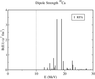
Figure 1: RPA dipole strength distribution for ⁴⁸Ca.

From the theoretical point of view, it has been found that relativistic and non-relativistic (Q)RPA models are not able to well describe the low-lying response in ⁴⁸Ca because they either do not provide the good excitation energies (too high energies) or do not predict the experimental fragmentation of the peaks. For example, in recent calculations performed with the relativistic RPA model no strength has been found in the response below the excitation energy of 10 MeV vret . The same kind of results is obtained in Skyrme SGII-RPA calculations (Fig. 1). On the other hand, a reasonable agreement (energies and fragmentation) with the experimental results has been found within the ETFFS model tre-1 ; tertychny where a quasiparticle-phonon coupling is included.

We perform SRPA calculations in spherical symmetry for the two isotopes ⁴⁰Ca and ⁴⁸Ca with the Skyrme interaction SGII. The technical details of these calculations are reported in Ref. gamba2010-1 . Differently from Ref. gamba2010-1 , the full rearrangement terms gamba2010-2 are used here in the SRPA matrices. Because of the zero-range of the Skyrme interaction, a natural energy cutoff is not provided. Different procedures to treat this problem may be envisaged for future studies (see, for instance, the exploratory work presented in Ref. moghrabi ). In this work, we have introduced an energy cutoff ($ECUT$) on the $2p2h$ configurations. By varying it from 40 to 60 MeV we have verified that a reasonable stability of the results is achieved around a cutoff of 50-55 MeV. The total $B(E1)$ and EWSRs values, integrated up to an energy of 10 MeV, are shown in Table 1 for the isotopes ⁴⁰Ca and ⁴⁸Ca as a function of the energy cutoff $ECUT$ on the $2p2h$ configurations.

The $B(E1)$ distributions for different choices of the energy cutoff are plotted in Fig. 2 up to an excitation energy of 10 MeV for the nucleus ⁴⁸Ca. The employed transition operator is

$$F_{10}=e_{p}\sum_{i=1}^{Z}r_{i}Y_{10}(\Omega_{i})-e_{n}\sum_{i=1}^{N}r_{i}Y_{10}(\Omega_{i})$$ (2)

where $e_{p}$ and $e_{n}$ are the kinematic charges, $e_{p}=Ne/A$ and $e_{n}=Ze/A$, respectively. One can observe that the results do not change strongly starting from a cutoff of 45 MeV. In what follows, we will analyze the results obtained with a cutoff of 60 MeV (bottom panel of Fig. 2).

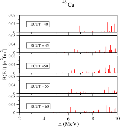
Figure 2: (Color online) SRPA dipole strength distribution for the ⁴⁸Ca isotope for increasing values of the energy cutoff $ECUT$ (MeV) on the $2p2h$ configurations included in the calculations.

	48Ca			40Ca
$ECUT$	$\sum B(E1)$	EWSRs		$\sum B(E1)$	EWSRs
40	0.184	1.623		0.009	0.091
45	0.218	1.895		0.002	0.022
50	0.226	1.944		0.015	0.139
55	0.240	2.049		0.025	0.237
60	0.230	1.964		0.023	0.211

Table 1: Total $B(E1)$ ($e^{2}fm^{2}$) and EWSRs ($e^{2}fm^{2}MeV$) integrated up to 10 MeV as a function of the energy cutoff $ECUT$ ($MeV$) on the $2p2h$ configurations for ⁴⁸Ca and ⁴⁰Ca.

These results are qualitatively of the same type as those found in Ref. tre-1 with the ETFFS approach which is also a beyond-mean-field model where the coupling is done with collective phonons instead of $2p2h$ configurations (as is done in SRPA). We can compare the location of the theoretical peaks with the experimental distribution (see, for instance, Fig. 2 of Ref. tre-1 ). We can distinguish two regions: from 6 to 8 MeV and from 8 to 10 MeV. Experimentally, the highest peak in the first region is found at $\sim$ 7 MeV whereas in our case we have several small peaks between 6 and 8 MeV and the highest peak is located around 6.2 MeV. In the interval between 8 and 10 MeV, our response is more fragmented than the experimental one. Experimentally, peaks are found around 8.5, 9 and 9.5 MeV. Our highest peak is located at $\sim$ 9.1 MeV. Finally, we have evaluated the response in the nucleus ⁴⁰Ca. Experimentally, a negligible strength has been found for this nucleus between 5 and 10 MeV (Fig. 2 of Ref. tre-1 ). Our results for ⁴⁰Ca are displayed in Fig. 3 for cutoff values varying from 40 up to 60 MeV. Some peaks are actually found at low energy but the corresponding strength is much lower than in ⁴⁸Ca (notice the different scales in the two figures).

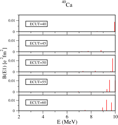
Figure 3: (Color online) As in Fig. 2 but for the ⁴⁰Ca isotope. Please note that a different scale has been used in the ordinate with respect to Fig. 2.

An interesting information that can be analyzed in connection with the strength distribution is the composition of the excitation modes in terms of $1p1h$ and $2p2h$ configurations. By extracting the expression of $N_{1}$ from the SRPA normalization condition,

$$\sum_{ph}(\mid X_{ph}^{\nu}\mid^{2}-\mid Y_{ph}^{\nu}\mid^{2})+\sum_{p<p^{\prime},h<h^{\prime}}(\mid X_{php^{\prime}h^{\prime}}^{\nu}\mid^{2}-\mid Y_{php^{\prime}h^{\prime}}^{\nu}\mid^{2})$$

$$=N_{1}+N_{2}=1,$$ (3)

we plot in Fig. 4 the $B(E1)$ values corresponding to a cutoff of 60 MeV (upper panel, same as in bottom panel of Fig. 2) and the quantity $N_{1}$ (lower panel) for each excitation of the nucleus ⁴⁸Ca. One observes that all the excitations present a mixing of $1p1h$ and $2p2h$ configurations. Those which have the highest $1p1h$ content (around 50%) may be interpreted as excitations that already exist in the RPA spectrum at higher energies (the first excitations in RPA are located around 11 MeV) and that are shifted down to lower energies due to the coupling with $2p2h$ configurations. In the SRPA spectrum we also see several states which present a dominant $2p2h$ nature and show a relatively large $B(E1)$ despite their very low content of $1p1h$ configurations (see for instance the energy region around 9 MeV).

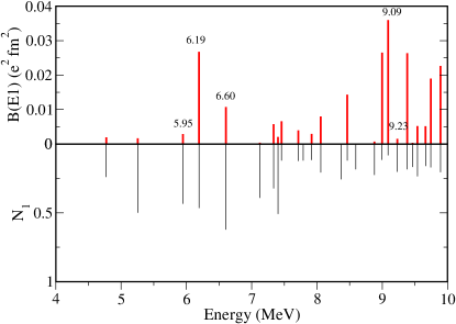
Figure 4: (Color online) For each state the $B(E1)$ value corresponding to a cutoff of 60 MeV (upper panel) and the total $1p1h$ contribution $N_{1}$ to the norm of the state defined in Eq. (3) (lower panel), are shown for ⁴⁸Ca.

As already mentioned in the Sec. I, low-energy excitations in light nuclei are mostly single-particle excitations and cannot be interpreted as a collective motion of a skin against a core. In Ca isotopes, which are intermediate cases between light and heavy nuclei, the nature of these excitations has not yet been clearly elucidated. In order to have a deeper insight into the properties of these low-energy modes we consider in more detail the states located at 5.95, 6.19 and 6.60 MeV as well as those located at 9.09 and 9.23 MeV. We can see that the first three states have a quite large and similar $1p1h$ component but show a very different $B(E1)$ value. In particular, one notices that the state located at 5.95 MeV has almost no strength. By comparing among themselves the states with energies 6.19 and 6.60 MeV, one observes that $N_{1}$ is larger while the $B(E1)$ value is about one half in the second state with respect to the first one. A different description is provided for the states lying at 9.09 and 9.23 MeV which are both almost entirely composed by $2p2h$ configurations. In spite of the fact that the $1p1h$ content is higher in the second state with respect to the first one, we notice that the second state has almost no strength while the first state is the most collective in the low-lying spectrum.

The nature of the low-energy peaks can be better analyzed by looking at the associated transition densities. In Fig. 5 we compare the transition densities corresponding to the peaks of 5.95 (upper panels), 6.19 (middle panels) and 6.60 (lower panels) MeV. For each state, we show separately the neutron $\delta\rho_{n}(r)$ and the proton $\delta\rho_{p}(r)$ (left), the isoscalar $\delta\rho_{n}(r)+\delta\rho_{p}(r)$ and the isovector $\delta\rho_{n}(r)-\delta\rho_{p}(r)$ (right) transitions densities. The same quantities are shown in Fig. 6 for the states located at 9.09 (upper panels) and 9.23 (lower panels) MeV.

In Table 2 we report for each state the isoscalar $B(E1,T=0)$ and isovector $B(E1,T=1)$ transition probabilities obtained by integrating the corresponding sets of Figs 5 and 6 multiplied by $r$. By looking at the transition densities of the first three states (Fig. 5) one does not see any clear signature of an oscillation of the neutron skin against the core at the surface of the nucleus. On the contrary, especially in the external part of the nucleus, the protons and neutrons oscillate in phase. For the state located at 5.95 MeV, the isoscalar and isovector transition densities strongly oscillate giving almost vanishing $B(E1,T=0)$ and $B(E1,T=1)$ values (see Table 2). A similar behavior is found for the state of 6.60 MeV. For the state lying at 6.19 MeV the cancellations are less important. Strong cancellations occur for the state located at 9.23 MeV, (lower panel of Fig. 6), resulting in very small $B(E1,T=0)$ and $B(E1,T=1)$ values (Table 2). A different situation is found for the most collective state located at 9.09 MeV. We see that the neutron transition density dominates over the proton one that is almost vanishing in the external part of the nucleus while in the interior the two densities oscillate out of phase. This leads to a strong mixing of isoscalar and isovector components.

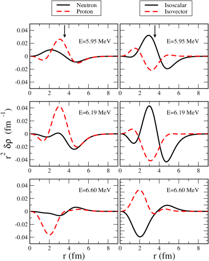
Figure 5: (Color online) Neutron and proton transition densities (left) and the corresponding isoscalar and isovector ones (right) associated to the peaks located at 5.95 (upper panels), 6.19 (middle panels) and 6.60 (lower panels) MeV.

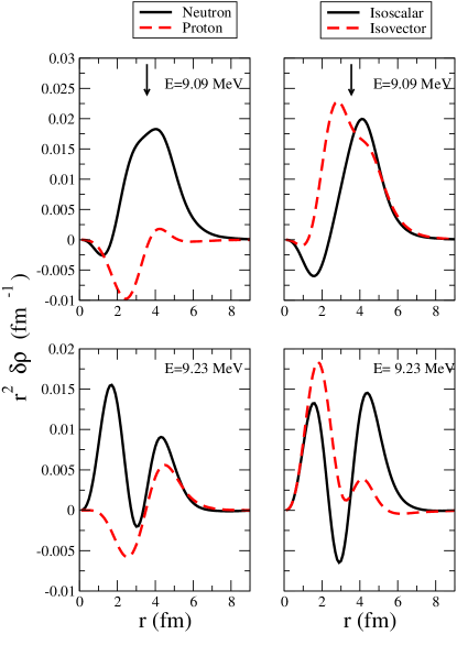
Figure 6: (Color online) As in Fig. 5 but for the states located at 9.09 and 9.23 MeV (upper and lower panels, respectively).

$E$ (MeV)	$B(E1,T=0)$	$B(E1,T=1)$
5.95	0.002	0.013
6.19	0.176	0.157
6.60	0.011	0.036
9.09	0.099	0.186
9.23	0.042	0.012

Table 2: Isoscalar $B(E1,T=0)$ ($e^{2}fm^{2}$) and isovector $B(E1,T=1)$ ($e^{2}fm^{2}$) transition probabilities obtained by integrating the corresponding curves shown in Figs 5 and 6 multiplied by $r$.

		$E=$ 5.95 MeV
$ph$ conf.	$E$ (MeV)	$A_{ph}$	$b_{ph}(E1)$	$F_{ph}^{\lambda}$
$(2p_{3/2},1d_{5/2})^{\pi}$	17.499	0.001	0.021	1.343
$(1f_{7/2},1d_{5/2})^{\pi}$	11.732	0.062	-0.470	3.304
$(2p_{3/2},2s_{1/2})^{\pi}$	12.444	0.022	0.140	1.726
$(2p_{1/2},2s_{1/2})^{\pi}$	14.133	0.004	0.043	-1.233
$(2p_{3/2},1d_{3/2})^{\pi}$	12.120	0.172	0.107	0.451
$(2p_{1/2},1d_{3/2})^{\pi}$	13.809	0.007	-0.050	1.053
$(1f_{5/2},1d_{3/2})^{\pi}$	13.867	0.012	0.188	2.756
$(2p_{3/2},2s_{1/2})^{\nu}$	11.773	0.006	0.060	1.737
$(2p_{1/2},2s_{1/2})^{\nu}$	13.556	0.001	-0.011	-1.248
$(2p_{3/2},1d_{3/2})^{\nu}$	10.329	0.145	-0.071	0.456
$(2p_{1/2},1d_{3/2})^{\nu}$	12.112	0.001	0.014	1.084
Partial Sum		0.433	-0.031
Total Sum		0.435	-0.054

Table 3: Particle-hole configurations which give the major contributions to the dipole low-lying state located at 5.95 MeV. For each $ph$ configuration, the energy, the contribution to the norm of the state $A_{ph}$, the partial contribution to the reduced transition amplitude $b_{ph}$ ($e$ fm) and the matrix element of the transition operator $F_{ph}^{\lambda}$ are reported. The superscripts $\pi$, $\nu$ refer to proton and neutron states, respectively.

		$E=$ 6.19 MeV
$ph$ conf.	$E$ (MeV)	$A_{ph}$	$b_{ph}(E1)$	$F_{ph}^{\lambda}$
$(1f_{7/2},1d_{5/2})^{\pi}$	11.732	0.156	-0.727	3.304
$(2p_{3/2},2s_{1/2})^{\pi}$	12.444	0.148	0.373	1.726
$(2p_{1/2},2s_{1/2})^{\pi}$	14.133	0.003	-0.043	-1.233
$(2p_{3/2},1d_{3/2})^{\pi}$	12.120	0.003	-0.015	0.451
$(2p_{1/2},1d_{3/2})^{\pi}$	13.809	0.073	0.166	1.053
$(1f_{5/2},1d_{3/2})^{\pi}$	13.867	0.018	0.250	2.756
$(2p_{3/2},1d_{5/2})^{\nu}$	15.683	0.000	0.012	1.410
$(2p_{3/2},2s_{1/2})^{\nu}$	11.773	0.015	-0.079	1.737
$(2p_{3/2},1d_{3/2})^{\nu}$	10.329	0.040	0.038	0.456
$(2p_{1/2},1d_{3/2})^{\nu}$	12.112	0.001	-0.016	1.084
$(1g_{9/2},1f_{7/2})^{\nu}$	11.364	0.003	-0.106	4.171
Partial Sum		0.461	-0.147
Total Sum		0.465	-0.163

Table 4: As in Table 3 but for the state located at 6.19 MeV

Another interesting analysis that can be done for these excitation modes is related to their collectivity in terms of number and coherence of the different $1p1h$ configurations which contribute the total transition probability. We present an analysis similar to that done in Ref. lanza . In SRPA as well as in RPA the reduced transition probability for a one-body operator describing the excitation from the ground state to a state $\nu$ can be written as

$$B(E\lambda)=|\sum_{ph}b_{ph}(E\lambda)|^{2}=|\sum_{ph}(X_{ph}^{\nu}-Y_{ph}^{\nu})F_{ph}^{\lambda}|^{2}$$ (4)

where $F_{ph}^{\lambda}$ are the multipole transition amplitudes associated to a $1p1h$ configuration. We remark that also in the case of SRPA only $1p1h$ amplitudes appear in the expression of the transition probability. A different situation would occur if a two-body operator is considered. In Refs. ni1 and roth , for example, the study of the double giant dipole resonance in ⁴⁰Ca and ¹⁶O has been carried out by using a two-body operator. In the spirit of a multiphonon picture, the latter is built as a product of two one-body dipole operators. As shown in Fig. 4, the low-lying dipole states that we obtain in SRPA have a strong $2p2h$ nature. It could thus be interesting to investigate their properties by using a two-body transition operator. In particular, the use of a transition operator containing both one-body and two-body terms is expected to affect the strength distribution and eventually the total strength associated to this energy region. On the other hand, it is not clear which kind of one-body multipole operators should be taken into account here to construct the two-body operator. This investigation is left as a subject for a future work.

In Tables 3-7 we report the particle-hole configurations which provide the major contributions to the dipole modes for the five states analyzed in Figs 5 and 6. For each configuration we report the unperturbed energy, the contribution $A_{ph}$ to the norm of the state,

$$A_{ph}=|X^{\nu}_{ph}|^{2}-|Y^{\nu}_{ph}|^{2},~{}~{}~{}\mbox{with}~{}~{}~{}\sum_{ph}A_{ph}=N_{1},$$ (5)

the partial contribution $b_{ph}$ to the reduced transition amplitude (see Eq. (4)) and the matrix element of the transition operator.

		$E=$ 6.60 MeV
$ph$ conf.	$E$ (MeV)	$A_{ph}$	$b_{ph}(E1)$	$F_{ph}^{\lambda}$
$(2p_{3/2},1d_{5/2})^{\pi}$	17.499	0.001	0.031	1.343
$(1f_{7/2},1d_{5/2})^{\pi}$	11.732	0.012	0.226	3.304
$(1f_{5/2},1d_{5/2})^{\pi}$	19.246	0.001	0.010	-0.734
$(2p_{3/2},2s_{1/2})^{\pi}$	12.444	0.190	0.421	1.726
$(2p_{1/2},2s_{1/2})^{\pi}$	14.133	0.002	-0.049	-1.233
$(2p_{1/2},1d_{3/2})^{\pi}$	13.809	0.335	-0.350	1.053
$(1f_{5/2},1d_{3/2})^{\pi}$	13.867	0.014	-0.193	2.756
$(2p_{3/2},2s_{1/2})^{\nu}$	11.773	0.005	-0.044	1.737
$(2p_{3/2},1d_{3/2})^{\nu}$	10.329	0.035	0.035	0.456
$(2p_{1/2},1d_{3/2})^{\nu}$	12.112	0.018	-0.060	1.084
$(2d_{5/2},1f_{7/2})^{\nu}$	12.698	0.001	0.015	1.212
$(3d_{5/2},1f_{7/2})^{\nu}$	15.625	0.000	0.010	1.055
$(1g_{9/2},1f_{7/2})^{\nu}$	11.364	0.001	0.058	4.171
Partial Sum		0.615	0.110
Total Sum		0.622	0.104

Table 5: As in Table 3 but for the state located at 6.60 MeV

We first briefly discuss the case of the RPA IVGDR whose collective features are well known. In Fig. 7 the partial contributions $b_{ph}$ corresponding to each $1p1h$ configuration for the first peak located at 17.33 MeV (Fig. 1) are shown. The bars correspond to each value of $b_{ph}$ associated to a single configuration while the continuous line is the cumulative sum of the contributions. The dashed line separates the proton from the neutron configurations which are ordered according to their increasing energy. We can clearly see that the contributions of many proton and neutron $1p1h$ configurations sum up coherently to provide the total $B(E1)$. This coherent behavior of protons and neutrons is due to the minus sign in the definition of the isovector transition operator, Eq. (2), and is not in contrast with the isovector character of this excitation where neutrons and protons oscillate out of phase.

In Figs. 8 and 9 the partial contributions $b_{ph}$ corresponding to each $1p1h$ configuration for the excitation modes located at 5.95, 6.19 and 6.60 MeV (Fig. 8) and at 9.09 and 9.23 MeV (Fig. 9) are plotted.

In the upper panel of Fig. 8 we see that, for the state lying at 5.95 MeV, several $1p1h$ configurations present non negligible $b_{ph}$ values. This is true especially for the proton configurations and is also indicated by the behavior of the proton transition density in Fig. 5. However, the total amplitude is very small since strong cancellations occur. The same holds for the state located at 6.19 MeV (middle panel of the same figure), but only for the proton $1p1h$ configurations whose cumulative sum is almost zero. The total transition amplitude is given in this case only by the neutron configurations. A different result is found for the third state shown in the lower panel, where the strong cancellation occurs for the neutron configurations. For the highest state lying at 9.23 MeV (lower panel of Fig. 9) we observe strong cancellations for both neutrons and protons leading to a very small total transition amplitude. A more interesting situation is obtained for the most collective state, located at 9.09 MeV (upper panel of Fig. 9). We observe also in this case a strong cancellation of the proton contributions while a quite coherent behavior is exhibited by the neutron $1p1h$ configurations. In particular, we observe strong contributions coming from the outermost neutrons (see also Table 6). This result, together with the profile of the corresponding transition density indicates that this state shows some features usually associated to pygmy resonances.

		$E=$ 9.09 MeV
$ph$ conf.	$E$ (MeV)	$A_{ph}$	$b_{ph}(E1)$	$F_{ph}^{\lambda}$
$(2p_{3/2},1d_{5/2})^{\pi}$	17.499	0.002	-0.039	1.343
$(1f_{7/2},1d_{5/2})^{\pi}$	11.732	0.001	-0.098	3.304
$(1f_{5/2},1d_{5/2})^{\pi}$	19.246	0.006	-0.032	-0.734
$(2p_{1/2},2s_{1/2})^{\pi}$	14.133	0.005	0.045	-1.233
$(2p_{3/2},1d_{3/2})^{\pi}$	12.120	0.007	-0.023	0.451
$(2p_{1/2},1d_{3/2})^{\pi}$	13.809	0.000	-0.014	1.053
$(1f_{5/2},1d_{3/2})^{\pi}$	13.867	0.017	0.197	2.756
$(2p_{3/2},1d_{5/2})^{\nu}$	15.683	0.006	-0.044	1.410
$(2p_{3/2},2s_{1/2})^{\nu}$	11.773	0.006	-0.055	1.737
$(2p_{1/2},2s_{1/2})^{\nu}$	13.556	0.001	-0.015	-1.248
$(2p_{3/2},1d_{3/2})^{\nu}$	10.329	0.011	-0.020	0.456
$(2p_{1/2},1d_{3/2})^{\nu}$	12.112	0.001	0.018	1.084
$(1f_{5/2},1d_{3/2})^{\nu}$	14.072	0.009	0.105	2.675
$(2d_{5/2},1f_{7/2})^{\nu}$	12.698	0.001	0.014	1.212
$(1g_{9/2},1f_{7/2})^{\nu}$	11.364	0.008	0.149	4.171
Partial Sum		0.082	0.189
Total Sum		0.083	0.190

Table 6: As in Table 3 but for the state of energy 9.09 MeV

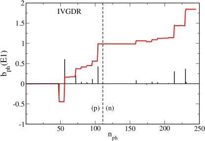
Figure 7: (Color online) Partial contributions $b_{ph}$ of the reduced transition probability versus the ordering number of the $1p1h$ configurations for the first peak of the RPA IVDGR located at 17.33 MeV (Fig. 1). The dashed line separates the proton from the neutron configurations. The configurations are ordered according to their increasing energy. The bars corresponds to the individual $b_{ph}$ contributions while the full red line is the cumulative sum of the contributions.

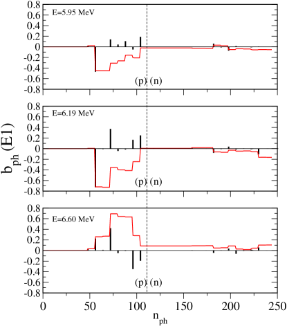
Figure 8: (Color online) As in Fig. 7 but for the state at at 5.95 MeV, 6.19 MeV and 6.60 MeV.

		$E=$ 9.23 MeV
$ph$ conf.	$E$ (MeV)	$A_{ph}$	$b_{ph}(E1)$	$F_{ph}^{\lambda}$
$(2p_{3/2},1d_{5/2})^{\pi}$	17.499	0.002	0.033	1.343
$(1f_{7/2},1d_{5/2})^{\pi}$	11.732	0.001	-0.059	3.304
$(2p_{3/2},2s_{1/2})^{\pi}$	12.444	0.000	-0.012	1.726
$(2p_{1/2},2s_{1/2})^{\pi}$	14.133	0.001	0.027	-1.233
$(2p_{3/2},1d_{3/2})^{\pi}$	12.120	0.023	0.040	0.451
$(2p_{3/2},1d_{5/2})^{\nu}$	15.683	0.008	-0.055	1.410
$(2p_{3/2},2s_{1/2})^{\nu}$	11.773	0.103	-0.226	1.737
$(2p_{1/2},2s_{1/2})^{\nu}$	13.556	0.001	0.019	-1.248
$(2p_{3/2},1d_{3/2})^{\nu}$	10.329	0.004	0.012	0.456
$(2p_{1/2},1d_{3/2})^{\nu}$	12.112	0.056	0.106	1.084
$(2d_{5/2},1f_{7/2})^{\nu}$	12.698	0.001	0.013	1.212
$(1g_{9/2},1f_{7/2})^{\nu}$	11.364	0.001	0.052	4.171
Partial Sum		0.201	-0.050
Total Sum		0.202	-0.037

Table 7: As in Table 3 but for the state lying at 9.23 MeV

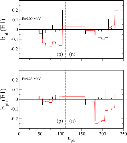
Figure 9: (Color online) As in Fig. 8 but for the state at 9.09 and 9.23 MeV (upper and lower panel, respectively). Please note that a different scale has been used in the ordinate with respect to Fig. 8.

		48Ca	40Ca
$\sum B(E1)$	SRPA	230	23
(10-3 e2 fm2)	Exp	68.7 $\pm$ 7.5	5.1 $\pm$ 0.8
$\sum_{i}E_{i}B_{i}(E1)$	SRPA	1964	211
10-3 e2 fm2 MeV	Exp	570 $\pm$ 62	35 $\pm$ 5
$E_{centroid}$	SRPA	8.54	9.17
MeV	Exp	8.40	6.80

Table 8: Total $B(E1)$ and EWSRs integrated up to 10 MeV and corresponding centroid energies obtained in SRPA compared with the experimental values tre-1 for the ^40,48Ca isotopes.

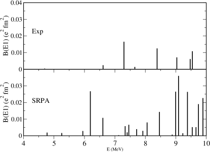
Figure 10: Comparison of the experimental B(E1) strength distribution tre-1 (upper panel) with the SRPA calculations (lower panel) for ⁴⁸Ca.

In Table 8 we compare the total $B(E1)$ and EWSRs integrated up to 10 MeV and the corresponding centroid energies with the experimental values tre-1 for the nuclei ⁴⁰Ca and ⁴⁸Ca. We see that the SRPA total $B(E1)$ is much larger, almost by a factor 4, than the experimental value. This is due to the larger number of states obtained in SRPA with respect to the experimental spectrum and, at the same time, to their higher strength (Fig. 10). The same kind of discrepancies is found for the EWSRs while the SRPA centroid energy is very close to the experimental value. Regarding these large differences some comments are in order. First we recall that, because of the non-local terms of the Skyrme interaction, the double commutator sum rule is enhanced with respect to the classical sum rule by a factor 1.35 for SGII. However, this is not enough to explain the strong deviation with respect to the experimental values. It could be also interesting to analyze whether or not this kind of discrepancy may depend on the choice of the Skyrme interaction. As a check, we have performed SRPA calculations by using the parametrization SLy4 and the same kind of deviations has been found. In a recent work colo it has been suggested that the low-lying dipole strength distribution could be be eventually related to the slope of the symmetry energy. This kind of analysis is however beyond our present scopes and it will be performed in future investigations. Finally, we recall that theoretical $B(E1)$ values much larger than the corresponding experimental results have also been found within the ETFFS model for the nucleus ⁴⁴Ca; it has been shown that this discrepancy is related to the use of some approximations in the treatment of pairing and continuum coupling tertychny . We also mention that in previous experimental measurements a much larger strength had been found in the energy region from 5 to 10 MeV Ottini . Finally, as mentioned above, since the low-lying dipole states obtained in SRPA have a strong $2p2h$ nature, it could more appropriate the use of a transition operator containing both one-body and two-body terms. Of course, the use of such a more general operator would affect the total strength associated to this energy region. This investigation is however left as a subject for a future work.

IV Mixing with the spurious state

Some comments about the spurious state and its possible mixing with the physical dipole modes are in order. The Thouless theorem on the EWSRs thou is very important in the framework of RPA and it holds also in SRPA yannou . It guarantees that spurious excitations corresponding to some symmetries separate out and are orthogonal to the physical states. This separation is obtained only in completely self-consistent calculations, that is, when the same interaction is used at both the HF and the RPA (or SRPA) level. In the case of dipole excitations, the center-of-mass motion should appear at zero energy and the EWSRs should be satisfied. Since the Coulomb and spin-orbit terms are not taken into account in the residual interaction, our calculations are not fully self-consistent and violations of the EWSRs are found (not larger than $2-3\%$). A currently adopted procedure to estimate the mixing with spurious components consists in using the isoscalar one-body operator corrected for the center-of-mass motion. This has been done, for example, in the study of giant resonances in Ref. gamba2010-1 . However, this check which is generally employed in RPA calculations is suitable to analyze excitations which are mainly composed by $1p1h$ states. In our case, as shown in Fig. 4, $1p1h$ and $2p2h$ components are strongly mixed and we thus choose a more appropriate procedure to estimate the mixing with spurious components.

The residual interaction has been multiplied by a renormalizing factor to shift to zero the energy of the spurious mode. In our RPA calculations, the spurious state lies at about 3.5 MeV exhausting more than 95% of the isoscalar EWSRs; by using a renormalizing factor of 1.09 its energy goes down to 0.2 MeV while the rest of the isoscalar and isovector distributions remains practically unaffected. In SRPA, as a consequence of the coupling with the $2p2h$ configurations, the spurious state is pushed down to lower energies with respect to RPA. Depending on the energy cutoff on the $2p2h$ configurations, its energy can be negative or imaginary in some cases. We stress that the use of the Hartree-Fock ground state that minimizes the energy guarantees that the RPA matrix is positive definite. This does not hold in SRPA. For the SRPA calculations with $ECUT=$ 60 MeV we have verified that, by using a renormalizing factor of 0.91, the spurious mode is located at about 0.12 MeV. The total $B(E1)$ (EWSRs) integrated up to 10 MeV does not change much when the renormalizing factor is introduced: from 0.230 $e^{2}$ fm² (1.964 $e^{2}$ fm² MeV) to 0.221 $e^{2}$ fm² (1.905 $e^{2}$ fm² MeV) . In Fig. 11 we show the dipole strength distribution obtained for the ⁴⁸Ca isotope without (full red lines) and with (dashed blue lines) the inclusion of the renormalizing factor in the residual interaction. Both calculations are done with an energy cutoff on the $2p2h$ configurations of 60 MeV. We see that the strength distribution is not strongly affected, the main difference being a shift of few hundreds KeV of some peaks and a change of their corresponding transition probability. This analysis seems to indicate that the presence of possible spurious components does not affect much our results.

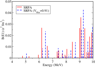
Figure 11: (Color online) Dipole strength distribution for the ⁴⁸Ca isotope obtained in SRPA without (full red lines) and with a renormalizing factor $V_{Rin}=0.91$ in the residual interaction (dashed blue lines). Both calculations are done with an energy cutoff on the $2p2h$ configurations of 60 MeV.

V Conclusions

In this work, we have analyzed the low-energy dipole spectrum (from 5 to 10 MeV) for the stable nuclei ⁴⁰Ca and ⁴⁸Ca in the framework of the Skyrme-SRPA model. The Skyrme interaction SGII is used. Almost no strength is found in this energy region for the nucleus ⁴⁰Ca whereas a non negligible strength is obtained for the neutron-rich nucleus ⁴⁸Ca. The distribution and the fragmentation of the peaks is in reasonable agreement with the corresponding experimental measurements. This kind of results cannot be provided by the standard RPA model: SGII-RPA calculations do not lead to any strength in the energy region from 5 to 10 MeV. However, we have found a $B(E1)$ value integrated up to 10 MeV which is quite larger than the corresponding experimental result.

The inclusion of $2p2h$ configurations and their coupling with the $1p1h$ ones and among themselves within SRPA has a two-fold effect on the low-lying dipole strength: (i) states that already exist in RPA are shifted to lower energies. These states maintain a quite strong $1p1h$ nature; (ii) several other states of almost pure $2p2h$ character appear. They are excited by the one-body dipole operator through their $1p1h$ components. In the nucleus ⁴⁸Ca one of these states shows the largest transition strength and displays some features generally associated with a dipole pygmy resonance.

A detailed analysis of the main excitations that compose the strength distributions is done: the content of $1p1h$ and $2p2h$ configurations is studied for some peaks. The transition densities are shown and the collectivity of the peaks is investigated in terms of the number and the coherence of the single configurations that mainly contribute. As far as the transition densities are concerned, one may conclude that in general they do not display the typical profile well known for pygmy resonances, except for the state located at 9.09 MeV. We have also observed that about 10-12 configurations contribute to each peak. In this sense one can say that there is some collectivity, however, strong cancellations occur in most cases and the single configurations do not sum up in a coherent way.

Our main conclusion is that, even if a low-lying dipole response is found experimentally and predicted theoretically in the isotope ⁴⁸Ca, one cannot really describe these excitations as pygmy resonances except for the most collective peak located at 9.09 MeV. This suggests that this nucleus is still too light to present clear signatures of an oscillation of the neutron skin against the internal core and that individual degrees of freedom are still dominant in the description of the dipole low-energy spectrum as for lighter nuclei.

References

- (1) N. Paar, D. Vretenar, E. Khan, and G. Colò, Rep. Prog. Phys. 70, 691 (2007).
- (2) T. Aumann, et al., Phys. Rev. C 59, 1252 (1999).
- (3) F. Catara, C. H. Dasso, and A. Vitturi, Nucl. Phys. A602, 181 (1996).
- (4) T. Aumann, et al., Nucl. Phys. A 649, 297c (1996); A. Leistenschneider, et al., Phys. Rev. Lett. 86, 5442 (2001); E. Tryggestad, et al., Nucl. Phys. A 687, 231c (2001); E. Tryggestad, et al., Phys. Lett. B 541, 52 (2002); E. Tryggestad, et al., Phys. Rev. C 67, 064309 (2003).
- (5) T. Hartmann, J. Enders, P. Mohr, K. Vogt, S. Volz, and A. Zilges, Phys. Rev. C 65, 034301 (2002).
- (6) T. Hartmann, M. Babilon, S. Kamerdzhiev, E. Litvinova, D. Savran, S. Volz, and A. Zilges, Phys. Rev. Lett. 93, 192501 (2004).
- (7) B. Özel, et al., Proceedings ox Comex2, Nucl. Phys. A 788, 385c (2007).
- (8) K. Govaert, et al., Phys. Rev. C 57, 2229 (1998).
- (9) P. Adrich, et al., Phys. Rev. Lett. 95, 132501 (2005).
- (10) N. Ryezayeva, et al. Phys. Rev. Lett. 89, 272502 (2002); T. Chapuran, et al., Phys. Rev. C 22, 1420 (1980); J. Enders, et al., Phys. Lett. B 486, 279 (2000); J. Enders, et al., Nucl. Phys. A 724, 243 (2003).
- (11) O. Wieland, et al., Phys. Rev. Lett. 102, 092502 (2009).
- (12) S. Péru, H. Goutte, and J.F. Berger, Nucl. Phys. A 788, 44 (2007).
- (13) N. Paar, Y.F. Niu, D. Vretenar, and J. Meng, Phys. Rev. Lett. 103, 032502 (2009).
- (14) G. Co’, V. De Donno, C. Maieron, M. Anguiano, and A. M. Lallena Phys. Rev. C 80, 014308 (2009)
- (15) I. Daoutidis and P. Ring, Phys. Rev. C 83, 044303 (2011)
- (16) M. Martini, S. Péru, and M. Dupuis, Phys. Rev. C 83, 034309 (2011)
- (17) E. Lanza, F. Catara, D. Gambacurta, V. Andrés, and Ph. Chomaz, Phys. Rev. C 79, 054615 (2009).
- (18) A. Vitturi, EG Lanza, MV Andres, F. Catara and D. Gambacurta, Pranama Journal of Physics, Vol. 75, (No.1), July 2010, 73
- (19) R. Mohan, M. Danos, and L.C. Biedenharn, Phys. Rev. C 3, 1740 (1971).
- (20) N. D. Dang, and A. Arima, Phys. Rev. Lett. 80, 4145 (1998).
- (21) G. Tertychny, et al., Nucl. Phys. A 788, 159c (2007).
- (22) N. Pillet, J.-F. Berger, and E. Caurier, Phys. Rev. C 78, 024305 (2008).
- (23) F. Andreozzi, F. Knapp, N. Lo Iudice, A. Porrino, and J. Kvasil, Phys. Rev. C 75, 044312 (2007).
- (24) M. Grasso, F. Catara, and M. Sambataro, Phys. Rev. C 66, 064303 (2002)
- (25) T. Hoshino and A. Arima, Phys. Rev. Lett. 37, 266 (1976)
- (26) W. Knupfer and M.G. Huber, Z. Phys. 276, 99 (1976)
- (27) S. Nishizaki and J. Wambach, Phys. Lett. B 349, 7 (1995)
- (28) S. Nishizaki and J. Wambach, Phys. Rev. C 57, 1515 (1998)
- (29) S. Adachi and S. Yoshida, Nucl. Phys. A 306, 53 (1978)
- (30) B. Schwesinger and J. Wambach, Phys. Lett. B 134, 29 (1984)
- (31) B. Schwesinger and J. Wambach, Nucl. Phys. A 426, 253 (1984)
- (32) S. Drozdz, V. Klemt, J. Speth, and J. Wambach, Nucl. Phys. A 451, 11 (1986)
- (33) S. Drozdz, V. Klemt, J. Speth, and J. Wambach, Phys. Lett. B 166, 18 (1986)
- (34) C. Yannouleas, M. Dworzecka, and J.J. Griffin, Nucl. Phys. A 397, 239 (1983)
- (35) C. Yannouleas and S. Jang, Nucl. Phys. A 455, 40 (1986)
- (36) P. Papakonstantinou, and R. Roth, Phys. Rev. C 81, 024317 (2010); Phys. Lett. B 671, 356 (2009).
- (37) D. Gambacurta, M. Grasso, and F. Catara, Phys. Rev. C 81, 054312 (2010).
- (38) D. Gambacurta, M. Grasso, and F. Catara, J. Phys. G: Nucl. and Part. Phys. 38, 035103 (2011).
- (39) C. Yannouleas, Phys. Rev. C 35, 1159 (1987).
- (40) M. Tohyama and M. Gong, Z. Phys. A 332, 269 (1989).
- (41) D. Lacroix, S. Ayik, and Ph. Chomaz, Prog. Part. Nucl. Phys. 52, 497 (2004).
- (42) J. da Providencia, Nucl. Phys. 61, 87 (1965).
- (43) R.H. McCamis, et al., Phys. Rev. C 33, 1624 (1986); R.F. Frosch, et al., Phys. Rev. 174, 1380 (1968).
- (44) D. Vretenar, N. Paar, P. Ring, and G.A. Lalazissis, Nucl. Phys. A 692, 496 (2001).
- (45) K. Moghrabi, M. Grasso, G. Colò, and N. Van Giai, Phys. Rev. Lett. 105, 262501 (2010).
- (46) A. Carbone, G. Coló, A. Bracco, L.G. Cao, P.F. Bortignon F. Camera and O. Wieland Phys. Rev. C 81, 041301(R) (2010)
- (47) S. Ottini-Hustache, N. Alamanos, F. Auger, B. Castel, Y. Blumenfeld, V. Chiste, N. Frascaria, A. Gillibert, C. Jouanne, V. Lapoux, F. Marie, W. Mittig, J. C. Roynette, and J. A. Scarpaci, Phys. Rev. C 59, 3429 (1999)
- (48) D. J. Thouless, Nucl. Phys. 21, 225 (1960).