Hard and soft walls

Abstract

In a continuing effort to understand divergences which occur when quantum fields are confined by bounding surfaces, we investigate local energy densities (and the local energy-momentum tensor) in the vicinity of a wall. In this paper, attention is largely confined to a scalar field. If the wall is an infinite Dirichlet plane, well known volume and surface divergences are found, which are regulated by a temporal point-splitting parameter. If the wall is represented by a linear potential in one coordinate $z$, the divergences are softened. The case of a general wall, described by a potential of the form $z^{\alpha}$ for $z>0$ is considered. If $\alpha>2$, there are no surface divergences, which in any case vanish if the conformal stress tensor is employed. Divergences within the wall are also considered.

I Introduction

Quantum vacuum energy, or Casimir energy, referring to the quantum energies of fields in the presence of material bodies or boundaries, is a mature subject Bordag:2009zz . In the last decade there have been tremendous advances in both experiment and theory, so that the so-called Lifshitz theory Lifshitz:1956zz has been confirmed at the 1% level, and theoretically there is now the possibility of calculating forces between bodies of practically any shape and constitution. Even the effects of finite temperature have now been confirmed Sushkov:2010cv . Yet, such effects are controversial, and there are many issues that are still unresolved.

One of the issues that has been controversial almost from the beginnings of the subject is that of the Casimir self-energy of an object, as opposed to the energy of interaction between two or more rigid objects. For example, in 1968 Boyer calculated the self-energy of a perfectly conducting spherical shell of zero thickness and found a surprising repulsive result Boyer:1968uf . This result has been confirmed by different techniques by many authors since. Yet within a decade, the meaning of this result was profoundly questioned Deutsch:1978sc ; not only is the meaning of self-energy rather obscure, but divergences occur whose omission has resulted in controversy up to the present time miltonself . Some of these divergences are proportional to the volume, to the surface area, and to the corners, so-called Weyl terms, which can be unambiguously removed. Curvature divergences are rather more subtle, and the reason Boyer obtained a finite result was that the interior and exterior curvature contributions cancel. Situations without curvature, such as triangular prisms Abalo:2010ah and tetrahedra Abalo2011 , have finite calculable self-energies when only the interior contributions are included.

The above calculations refer to the total energies of the systems. Yet, there is much interest in local quantum energy densities, or more generally, the vacuum expectation value of the stress-energy tensor. There are well-known divergences in these as surfaces are approached miltonself . However, most of the work on this subject has studied perfect boundaries, such as ideal conductors or Dirichlet walls. Since there are still issues regarding surface divergences that are not well understood, which are particularly relevant when the coupling to gravity is considered, in this paper we will consider walls that are modeled by potentials that are “softer” than such a perfect wall. (Soft walls were considered earlier, but apparently only for the global energy actor .) In particular, we will consider massless scalar fields in three dimensions in the presence of a potential which depends only on one coordinate, $z$. We follow Bouas et al. fulling and consider semi-infinite potentials, so that the potential vanishes for $z<0$ while it is a monomial in $z$ for $z>0$. For special cases (Dirichlet, linear, and quadratic potentials) the energy density may be found explicitly in terms of known functions, but in general asymptotics yield the information about the nature of the divergences as the region of the potential is approached from the left, as well as the divergences in the region of the potential. Unlike many previous investigations of this subject, including some by Milton miltonbook ; miltonself , we precisely regulate all expressions by inserting a temporal point-splitting. Then precise forms of the divergences in terms of the temporal splitting parameter are obtained, which exhibit the expected Weyl terms, as well as the nature of the singularity at the boundary $z=0$. Unlike Ref. fulling we consider a general stress tensor with arbitrary conformal parameter $\xi$; that reference considers $\xi=1/4$, but we find that for $\xi=1/6$ the divergences that occur as the boundary is approached are removed; in any case, they disappear for a potential higher than quadratic.

II Dirichlet Wall

Consider a massless scalar field in three-dimensional space subject to a Dirichlet wall

$$v(z)=\left\{\begin{array}[]{cc}0,&z<0,\\ \infty,&z>0.\end{array}\right.$$ (1)

The Green’s function, the solution to

$$\left(\frac{\partial^{2}}{\partial t^{2}}-\nabla^{2}+v\right)G(x,x^{\prime})=\delta(x-x^{\prime}),$$ (2)

has the form

$$G(x,x^{\prime})=\int\frac{d\omega}{2\pi}\frac{(d\mathbf{k_{\perp}})}{(2\pi)^{2}}e^{-i\omega(t-t^{\prime})}e^{i\mathbf{k_{\perp}\cdot(r-r^{\prime})_{\perp}}}g(z,z^{\prime};\kappa),$$ (3)

where, for $z,z^{\prime}<0$,

$$g(z,z^{\prime},\kappa)=-\frac{1}{\kappa}e^{\kappa z_{<}}\sinh\kappa z_{>},$$ (4)

where $z_{<}$, $z_{>}$ is the lesser, greater of $z$ and $z^{\prime}$. Here

$$\kappa^{2}=k_{\perp}^{2}-\omega^{2},$$ (5)

where we have anticipated making the Euclidean rotation (not just a Wick rotation)

$$\omega\to i\zeta,\quad(t-t^{\prime})\to i\tau,$$ (6)

so we may regard $\kappa$ as positive.

The energy-momentum tensor for the scalar field is

$$t^{\mu\nu}=\partial^{\mu}\phi\partial^{\nu}\phi-\frac{1}{2}g^{\mu\nu}\left(\partial_{\lambda}\phi\partial^{\lambda}\phi\right)-\xi\left(\partial^{\mu}\partial^{\nu}-g^{\mu\nu}\partial^{2}\right)\phi^{2},$$ (7)

where $\xi$ the conformal parameter, which for the conformal value of $\xi=\frac{1}{6}$ yields a traceless stress tensor, $t^{\lambda}{}_{\lambda}=0$. The connection between the classical causal (Feynman) Green’s function and the (time-ordered) vacuum expectation values of the fields is

$$\langle\phi(x)\phi(x^{\prime})\rangle=\frac{1}{i}G(x,x^{\prime}),$$ (8)

so the one-loop vacuum energy density of the field is

$$u(z)=\langle t^{00}\rangle=\frac{1}{2i}\left(\partial^{0}\partial^{\prime 0}+\bm{\nabla\cdot\nabla^{\prime}}\right)G(x,x^{\prime})\bigg{|}_{x^{\prime}\to x}+i\xi\nabla^{2}G(x,x).$$ (9)

Using the Fourier representation (3) we have for the energy density

$$u(z)=\frac{1}{2}\int\frac{d\zeta}{2\pi}\frac{(d\mathbf{k_{\perp}})}{(2\pi)^{2}}e^{i\zeta\tau}\left[\left(-\zeta^{2}+k_{\perp}^{2}+\frac{\partial}{\partial z}\frac{\partial}{\partial z^{\prime}}\right)g(z,z^{\prime})\bigg{|}_{z^{\prime}\to z}-2\xi\frac{\partial^{2}}{\partial z^{2}}g(z,z)\right].$$ (10)

Here, we have regulated the integral by retaining $\tau$ as a temporal point-splitting regulator, to be set equal to zero at the end of the calculation. We now introduce polar coordinates in the $\zeta$-$\mathbf{k}$ volume, so that

$$\zeta=\kappa\cos\theta,\quad|\mathbf{k_{\perp}}|=\kappa\sin\theta$$ (11)

and then the integral over the regulator term is

$$\int_{-1}^{1}d\cos\theta\,e^{i\tau\kappa\cos\theta}=\frac{2}{\kappa\tau}\sin\kappa\tau.$$ (12)

Inserting the Green’s function (4) into the energy integral (10) yields

$$\frac{1}{8\pi^{2}}\int_{0}^{\infty}d\kappa\,\kappa^{3}\left[e^{2\kappa z}\left(4\xi-1-\frac{1}{\kappa^{2}}\frac{\partial^{2}}{\partial\tau^{2}}\right)+\frac{1}{\kappa^{2}}\frac{\partial^{2}}{\partial\tau^{2}}\right]\frac{2}{\kappa\tau}\sin\kappa\tau.$$ (13)

The two terms in Eq. (13) consist of a $z$-dependent term and a constant. The latter is just the bulk energy density arising from the free part of the Green’s function,

$$g_{0}(z,z^{\prime})=\frac{1}{2\kappa}e^{-\kappa|z-z^{\prime}|}.$$ (14)

This is evaluated as

$$u_{0}=\frac{1}{4\pi^{2}}\frac{\partial^{2}}{\partial\tau^{2}}\frac{1}{\tau}\int_{0}^{\infty}d\kappa\sin\kappa\tau=\frac{3}{2\pi^{2}\tau^{4}},$$ (15)

which uses the integral

$$\int_{0}^{\infty}dx\,\sin x=1.$$ (16)

This result is just the well-known volume Weyl term. If $|z|\gg\tau$, we can take $\tau\to 0$ in the remaining term, and we find for the Dirichlet wall

$$u(z)-u_{0}=-\frac{1-6\xi}{6\pi^{2}}\int_{0}^{\infty}d\kappa\,\kappa^{3}e^{2\kappa z}=-\frac{1-6\xi}{16\pi^{2}z^{4}}.$$ (17)

This is exactly the form found near one of the plates for the two-plate Casimir situation miltonbook ; miltonself . Note that this term vanishes for $\xi=1/6$, which suggests that it has no significance, disregarding gravity. If we keep the regulator, we can integrate over the whole volume to the left of the wall:

$$\int_{-\infty}^{0}dz(u-u_{0})=\frac{1}{8\pi^{2}}\int_{0}^{\infty}d\kappa\,\kappa^{2}\left[4\xi\frac{\sin\kappa\tau}{\kappa\tau}+2\frac{\cos\kappa\tau}{(\kappa\tau)^{2}}-2\frac{\sin\kappa\tau}{(\kappa\tau)^{3}}\right]=-\frac{1}{8\pi\tau^{3}}.$$ (18)

This uses the evaluations

$$\int_{0}^{\infty}d\kappa\cos\kappa\tau=0,\quad\int_{0}^{\infty}d\kappa\,\kappa\sin\kappa\tau=0,\quad\int_{0}^{\infty}\frac{d\kappa}{\kappa}\sin\kappa\tau=\frac{\pi}{2}.$$ (19)

The result (18) is exactly the second Weyl term, expressing the energy per unit area for a Dirichlet wall.

In exactly the same way we can compute all the components of the stress tensor. The result, for $|z|\gg\tau$, is exactly as expected:

$$\langle t^{\mu\nu}\rangle=\frac{1}{2\pi^{2}\tau^{4}}\mbox{diag}(3,1,1,1)+\frac{1-6\xi}{16\pi^{2}z^{4}}\mbox{diag}(-1,1,1,0).$$ (20)

The bulk term has the required traceless, rotationally-invariant form, since it is unaware of the wall. The surface-divergent term vanishes for the conformal case, and exhibits no force on the wall, so is unobservable. This stress tensor trivially satisfies energy-momentum conservation, $\partial_{\mu}\langle t^{\mu\nu}\rangle=0$.

Incidentally, note that if the cutoff were omitted for the bulk term, we would obtain a form that is consistent not with rotational symmetry, but with the symmetry for the $2+1$ dimensional breakup as seen in the finite part of the stress tensor for the interaction between two Dirichlet plates:

$$u_{0}\to-\frac{1}{12\pi^{2}}\int_{0}^{\infty}d\kappa\,\kappa^{3}\mbox{diag}(1,-1,-1,3).$$ (21)

III Linear Wall

We next consider the linear wall,

$$v(z)=\left\{\begin{array}[]{cc}0,&z<0.\\ z,&z>0.\end{array}\right..$$ (22)

The energy density to the left of the wall is given by Eq. (10), whereas to the right of the wall, the potential must be included, or in general

$$u(z) = \frac{1}{2}\langle\left[(\partial^{0}\phi)^{2}+\bm{\nabla}\phi\cdot\bm{\nabla}\phi+v\phi^{2}\right]-2\xi\nabla^{2}\phi^{2}]\rangle.$$ (23)

In Eq. (23) the fields are to be evaluated at coincident points, and again the connection with the Green’s function is given by Eqs. (8) and (3), where now the reduced Green’s function satisfies

$$\left(-\frac{\partial^{2}}{\partial z^{2}}+k^{2}+v(z)-\omega^{2}\right)g(z,z^{\prime})=\delta(z-z^{\prime}).$$ (24)

As we saw before, it is convenient to perform a Euclidean rotation, $\omega\to i\zeta$.

To find the energy density for the region to the left of the wall, $z<0$, we solve Eq. (24) in the two regions, always assuming $z^{\prime}<0$, in terms of the variable $\kappa^{2}=k^{2}+\zeta^{2}$:

$$z<0:\quad g(z,z^{\prime}) = \frac{1}{2\kappa}e^{-\kappa|z-z^{\prime}|}+A(z^{\prime})e^{\kappa z},$$ (25a)

$$z>0:\quad g(z,z^{\prime}) = B(z^{\prime})\mbox{Ai}(\kappa^{2}+z).$$ (25b)

Here we have chosen the boundary conditions that as $z\to\pm\infty$, the Green’s function must vanish. The functions $A$ and $B$ are determined by the requirement that the function and its derivative must be continuous at $z=0$. This leads to two equations

$$B(z^{\prime})\mbox{Ai}(\kappa^{2}) = \frac{1}{2\kappa}e^{\kappa z^{\prime}}+A(z^{\prime}),$$ (26a)

$$\frac{1}{\kappa}B(z^{\prime})\mbox{Ai}^{\prime}(\kappa^{2}) = -\frac{1}{2\kappa}e^{\kappa z^{\prime}}+A(z^{\prime}),$$ (26b)

which may be immediately solved:

$$A(z^{\prime}) = \frac{1}{2\kappa}e^{\kappa z^{\prime}}\frac{1+\mbox{Ai}^{\prime}(\kappa^{2})/\kappa\mbox{Ai}(\kappa^{2})}{1-\mbox{Ai}^{\prime}(\kappa^{2})/\kappa\mbox{Ai}(\kappa^{2})},$$ (27a)

$$B(z^{\prime}) = \frac{e^{\kappa z^{\prime}}}{\kappa\mbox{Ai}(\kappa^{2})-\mbox{Ai}^{\prime}(\kappa^{2})}.$$ (27b)

Thus, in particular, the reduced Green’s function in the potential-free region is

$$z,z^{\prime}<0:\quad g(z,z^{\prime}) = \frac{1}{2\kappa}e^{-\kappa|z-z^{\prime}|}+\frac{1}{2\kappa}e^{\kappa(z+z^{\prime})}\frac{1+\mbox{Ai}^{\prime}(\kappa^{2})/\kappa\mbox{Ai}(\kappa^{2})}{1-\mbox{Ai}^{\prime}(\kappa^{2})/\kappa\mbox{Ai}(\kappa^{2})}.$$ (28)

When we insert this into the expression for the energy density (10) we omit the vacuum term in the Green’s function, since that has no knowledge of the potential, and was completely analyzed in the previous section. We are left with for $z<0$ ($|z|\gg\tau$)

$$u(z)-u_{0}=\frac{1-6\xi}{6\pi^{2}}\int_{0}^{\infty}d\kappa\,\kappa^{3}e^{2\kappa z}\frac{1+\mbox{Ai}^{\prime}(\kappa^{2})/\kappa\mbox{Ai}(\kappa^{2})}{1-\mbox{Ai}^{\prime}(\kappa^{2})/\kappa\mbox{Ai}(\kappa^{2})}.$$ (29)

Unlike the integral over real phase shifts fulling , the integrand is monotonically tending to zero as $\kappa\to\infty$. The integral is therefore finite for all $z<0$, and may be very easily evaluated by Mathematica. The results are shown in Fig. 1. It is seen that the energy density diverges as $z\to 0$, not at $z=1$; in fact, by using the asymptotic expansion of the Airy function,

$$\frac{1+\mbox{Ai}^{\prime}(\kappa^{2})/\kappa\mbox{Ai}(\kappa^{2})}{1-\mbox{Ai}^{\prime}(\kappa^{2})/\kappa\mbox{Ai}(\kappa^{2})}\sim-\frac{1}{8\kappa^{3}},\quad\kappa\to\infty,$$ (30)

it behaves for small negative $z$ like

$$u\sim\frac{1-6\xi}{96\pi^{2}}\frac{1}{z}.$$ (31)

The comparison with the exact numerical integration with this leading asymptotic behavior is also shown in Figs. 1, 2.

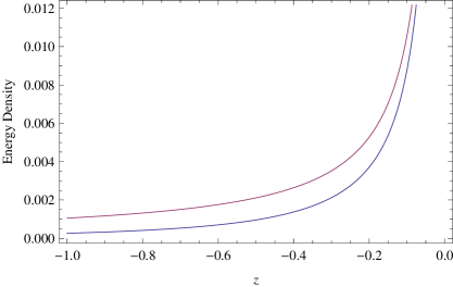
Figure 1: Energy density (divided by $6\xi-1$) to the left of a linear potential. The exact result (lower curve) is compared with the asymptotic behavior for small $z$, Eq. (31).

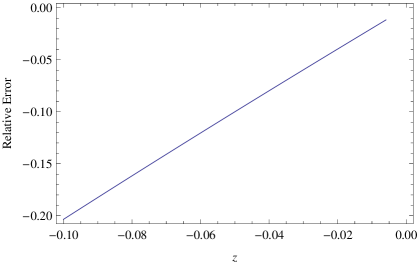
Figure 2: Relative error of the asymptotic approximation (31).

The solution for the Green’s function inside the wall is

$$0<z,z^{\prime}:\quad g(z,z^{\prime})=\pi\mbox{Ai}(\kappa^{2}+z_{>})\mbox{Bi}(\kappa^{2}+z_{<})-\frac{(\kappa\mbox{Bi}-\mbox{Bi}^{\prime})(\kappa^{2})}{(\kappa\mbox{Ai}-\mbox{Ai}^{\prime})(\kappa^{2})}\pi\mbox{Ai}(\kappa^{2}+z)\mbox{Ai}(\kappa^{2}+z^{\prime}).$$

(32)

The energy density within the wall is given by Eq. (23), or

$$u = \frac{1}{8\pi^{2}}\int_{0}^{\infty}d\kappa\,\kappa^{2}\int_{-1}^{1}d\cos\theta\bigg{\{}\left[\kappa^{2}+2\frac{\partial^{2}}{\partial\tau^{2}}+z\right]g(z,z)$$ (33)

$$\quad\mbox{}+\frac{\partial}{\partial z}\frac{\partial}{\partial z^{\prime}}g(z,z^{\prime})\big{|}_{z^{\prime}\to z}-2\xi\frac{\partial^{2}}{\partial z^{2}}g(z,z)\bigg{\}}e^{i\kappa\tau\cos\theta}.$$

Because both terms in $g$ involve Airy functions of argument $\kappa^{2}+z$, we can use the differential equation for the Airy function to write the above as

$$u=\frac{1}{8\pi^{2}}\left[(1-4\xi)\frac{\partial^{2}}{\partial z^{2}}+4\frac{\partial^{2}}{\partial\tau^{2}}\right]\int_{0}^{\infty}d\kappa\,\kappa\,g(z,z)\frac{\sin\kappa\tau}{\tau}.$$ (34)

Let us analyze the divergence structure, by considering the first term in $g$, Eq. (32), which would be the term arising if the linear potential existed over all space, because $\mbox{Ai}(z)\to 0$ as $z\to\infty$, while $\mbox{Bi}(z)\to 0$ as $z\to-\infty$. In any case, this term corresponds to the bulk energy density

$$\tilde{u}_{0}=\frac{1}{8\pi^{2}}\left[(1-4\xi)\frac{\partial^{2}}{\partial z^{2}}+4\frac{\partial^{2}}{\partial\tau^{2}}\right]\int_{0}^{\infty}d\kappa\,\kappa\pi\mbox{Ai}(\kappa^{2}+z)\mbox{Bi}(\kappa^{2}+z)\frac{\sin\kappa\tau}{\tau}.$$ (35)

To see the divergence structure, use the leading asymptotic behavior

$$\pi\mbox{Ai}(\kappa^{2}+z)\mbox{Bi}(\kappa^{2}+z)\sim\frac{1}{2}\frac{1}{\sqrt{\kappa^{2}+z}},$$ (36)

for large $\kappa$. Then we write the resulting $\kappa$ integral as

$$\int_{0}^{\infty}d\kappa\,\kappa\frac{1}{\sqrt{\kappa^{2}+z}}\sin\kappa\tau=\sqrt{z}\int_{0}^{\infty}dy\sin\left(\sqrt{y^{2}-1}\sqrt{z}\tau\right),$$ (37)

which for small $\tau$ is dominated by large $y$, so that the integral can be approximated by

$$\sqrt{z}\int_{1}^{\infty}dy\left\{\left(1-\frac{z\tau^{2}}{8y^{2}}\right)\sin y\sqrt{z}\tau-\frac{\sqrt{z}\tau}{2y}\left(1+\frac{1}{4y^{2}}\right)\cos y\sqrt{z}\tau\right\}.$$ (38)

The required integrals are, for small $\beta$,

$$\int_{1}^{\infty}dy\sin\beta y = \frac{1}{\beta},\quad\int_{1}^{\infty}dy\frac{\sin\beta y}{y^{2}}=-\beta\ln\beta+\mathscr{O}(\beta),$$ (39a)

$$\int_{1}^{\infty}dy\frac{\cos\beta y}{y} = -\ln\beta+\mbox{constant},\quad\int_{1}^{\infty}dy\frac{\cos\beta y}{y^{3}}=\frac{\beta^{2}}{2}\ln\beta+\mathscr{O}(\beta^{2})$$ (39b)

and then we see only the $\tau$ derivative term contributes in Eq. (35), and we obtain the expected result fulling

$$\tilde{u}_{0}\sim\frac{3}{2\pi^{2}}\frac{1}{\tau^{4}}-\frac{z}{8\pi^{2}\tau^{2}}+\frac{z^{2}}{32\pi^{2}}\ln\tau,$$ (40)

as the cutoff $\tau\to 0$. (Our point-splitting procedure would probably not reveal a possible $\delta$-function contribution suggested in Ref. fulling .)

IV General $z^{\alpha}$ potential

In general, for an $\alpha$ wall, described by the potential

$$v(z)=\left\{\begin{array}[]{cc}0,&z<0,\\ z^{\alpha},&z>0,\end{array}\right.$$ (41)

with $\alpha>0$, we construct the reduced Green’s function in terms of the two independent solutions in the region of the potential

$$\left(-\frac{\partial^{2}}{\partial z^{2}}+\kappa^{2}+z^{\alpha}\right)\left\{\begin{array}[]{c}F(z)\\ G(z)\end{array}\right.=0,$$ (42)

where $F(z)$ is chosen to vanish as $z\to+\infty$, and $G(z)$ is an arbitrary independent solution. The Wronskian is

$$w=F(z)G^{\prime}(z)-G(z)F^{\prime}(z),$$ (43)

which is just a constant.

The Green’s function to the left of the wall is

$$z,z^{\prime}<0,\quad g(z,z^{\prime})=\frac{1}{2\kappa}e^{-\kappa|z-z^{\prime}|}+\frac{1}{2\kappa}e^{\kappa(z+z^{\prime})}\frac{F(0)+F^{\prime}(0)/\kappa}{F(0)-F^{\prime}(0)/\kappa},$$ (44)

and to the right of the wall,

$$z,z^{\prime}>0:\quad g(z,z^{\prime})=\frac{1}{w}F(z_{>})G(z_{<})-\frac{1}{w}F(z)F(z^{\prime})\frac{G(0)-G^{\prime}(0)/\kappa}{F(0)-F^{\prime}(0)/\kappa}.$$ (45)

(Adding an arbitrary multiple of $F$ to $G$, of course, leaves this expression unchanged.)

For $\alpha=1$, $F(z)=\mbox{Ai}(\kappa^{2}+z)$, $G(z)=\mbox{Bi}(\kappa^{2}+z)$, and $w=1/\pi$, and we recover the result in the previous section. For $\alpha=2$, $F(z)=U(\kappa^{2}/2,\sqrt{2}z)$, $G(z)=U(\kappa^{2}/2,-\sqrt{2}z)$, in terms of the parabolic cylinder function NIST ; Bender . Alternative notations for this function are

$$U(a,x)=D_{-a-1/2}(x).$$ (46)

The value of the parabolic cylinder function, and its derivative, at the origin is

$$D_{\nu}(0) = \sqrt{\pi}2^{\nu/2}/\Gamma(1/2-\nu/2),$$ (47a)

$$D^{\prime}_{\nu}(0) = -\sqrt{\pi}e^{\nu/2+1/2}/\Gamma(-\nu/2).$$ (47b)

Therefore, the Wronskian is

$$w=\frac{\pi 2^{3/2-\kappa^{2}/2}}{\Gamma(\kappa^{2}/4+1/4)\Gamma(\kappa^{2}/4+3/4)}.$$ (48)

The energy density to the left of the wall, $z<0$, is immediately generalized from Eq. (29):

$$u(z)-u_{0}=\frac{1-6\xi}{6\pi^{2}}\int_{0}^{\infty}d\kappa\,\kappa^{3}\,e^{2\kappa z}\frac{F(0)+F^{\prime}(0)/\kappa}{F(0)-F^{\prime}(0)/\kappa}.$$ (49)

For the quadratic wall

$$\frac{F(0)+F^{\prime}(0)/\kappa}{F(0)-F^{\prime}(0)/\kappa}=\frac{1-\frac{2}{\kappa}\frac{\Gamma(\kappa^{2}/4+3/4)}{\Gamma(\kappa^{2}/4+1/4)}}{1+\frac{2}{\kappa}\frac{\Gamma(\kappa^{2}/4+3/4)}{\Gamma(\kappa^{2}/4+1/4)}}.$$ (50)

Asymptotically,

$$\frac{\Gamma(\kappa^{2}/4+3/4)}{\Gamma(\kappa^{2}/4+1/4)}\sim\frac{\kappa}{2}\left(1+\frac{1}{4\kappa^{4}}\right),\quad\kappa\to\infty,$$ (51)

so we approximate the exact energy density to the left of the wall by

$$u(z)-u_{0}\sim-\frac{1-6\xi}{6\pi^{2}}\int_{1}^{\infty}\frac{d\kappa}{8\kappa}e^{2\kappa z}=-\frac{1-6\xi}{48\pi^{2}}\Gamma(0,-2z),$$ (52)

in terms of the incomplete gamma function. The latter is actually a very accurate approximation as Fig. 3 shows.

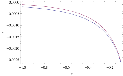
Figure 3: The lower curve shows the exact energy density for the quadratic wall, for $z<0$, using Eq. (49) with Eq. (50). The upper curve is the asymptotic approximation to that energy density, given by Eq. (52). Again the factor $6\xi-1$ is divided out.

In the region of the potential, we can calculate the generalization of the “bulk energy” (35),

$$\tilde{u}_{0}=\frac{1}{8\pi^{2}}\left[(1-4\xi)\frac{\partial^{2}}{\partial z^{2}}+4\frac{\partial^{2}}{\partial\tau^{2}}\right]\int_{0}^{\infty}d\kappa\,\kappa\,\tilde{g}_{0}(z,z)\frac{\sin\kappa\tau}{\tau},$$ (53)

because the argument leading from Eq. (33) to Eq. (34) holds for an arbitrary potential. Here, for the quadratic wall,

$$\tilde{g}_{0}(z,z^{\prime})=\frac{1}{w}U(\kappa^{2}/2,\sqrt{2}z)U(\kappa^{2}/2,-\sqrt{2}z).$$ (54)

The uniform asymptotic approximation for large order for $U(\kappa^{2}/2,\sqrt{2}\kappa t)$ is given in the NIST handbook NIST . The leading approximation is rather immediately found to yield

$$\tilde{g}_{0}(z,z)\sim\frac{1}{2\sqrt{\kappa^{2}+z^{2}}}-\frac{1}{8}\frac{1}{(\kappa^{2}+z^{2})^{5/2}}+\dots,$$ (55)

where the subleading term is explained in the following. The leading term differs from Eq. (36) simply by changing the potential from $z$ to $z^{2}$. This means that we can make the same substitution in the integral (38), and so the bulk energy density (53) is

$$\tilde{u}_{0}=\frac{3}{2\pi^{2}}\frac{1}{\tau^{4}}-\frac{1}{8\pi^{2}}\frac{z^{2}}{\tau^{2}}+\frac{1}{32\pi^{2}}\left[z^{4}+2(1-4\xi)-\frac{2}{3}\right]\ln\tau,$$ (56)

where the $-(2/3)\ln\tau$ term arising from the subleading term in Eq. (55) results in the appearance of the conformal coefficient $(4/3)(1-6\xi)$ for the constant term multiplying $\ln\tau$. This last result may be easily generalized to an arbitrary potential $v(z)$. The bulk Green’s function at coincident points can be written as

$$\tilde{g}_{0}(z,z)=\frac{1}{G^{\prime}(z)/G(z)-F^{\prime}(z)/F(z)}.$$ (57)

The leading asymptotic behavior of the solutions is given by the WKB approximation Bender ,

$$F(z) \sim Q^{-1/4}(z)\exp\left[-\int^{z}dt\left(Q^{1/2}(t)+\frac{v^{\prime\prime}(t)}{8Q^{3/2}(t)}\right)\right],$$ (58a)

$$G(z) \sim Q^{-1/4}(z)\exp\left[\int^{z}dt\,\left(Q^{1/2}(t)+\frac{v^{\prime\prime}(t)}{8Q^{3/2}(t)}\right)\right],$$ (58b)

where $Q(z)=\kappa^{2}+v(z)$. Here it was necessary to keep the first subleading correction, as given in Ref. Bender . Thus, for large $\kappa$,

$$\frac{G^{\prime}(z)}{G(z)}-\frac{F^{\prime}(z)}{F(z)}\sim 2Q^{1/2}(z)\left(1+\frac{v^{\prime\prime}(z)}{8Q^{2}(z)}\right).$$ (59)

This is the immediate generalization of Eqs. (36) and (55). Then, the generalization of the Weyl expansion (40) and (56) is

$$\tilde{u}_{0}\sim\frac{3}{2\pi^{2}}\frac{1}{\tau^{4}}-\frac{1}{8\pi^{2}}\frac{v}{\tau^{2}}+\frac{1}{32\pi^{2}}\left[v^{2}+\frac{2}{3}(1-6\xi)\frac{\partial^{2}}{\partial z^{2}}v\right]\ln\tau,$$ (60)

which uses the evaluation

$$\int_{0}^{\infty}\frac{d\kappa\,\kappa}{(\kappa^{2}+v)^{5/2}}\sin\kappa\tau\sim\frac{1}{6}\tau^{3}\ln\tau,$$ (61)

which follows from Eq. (39a). Note that the derivative term vanishes for the conformal value of $\xi$. This form, of course, follows from the general heat kernel consideration of this problem, and is seen for $\xi=1/4$ in Ref. fulling .

The behavior of the energy density to the left of the wall is also worked out easily, in general. We rescale the equation (42) for $F(z)$, so that $z=x/\kappa$,

$$\left(-\frac{d^{2}}{dx^{2}}+1+\kappa^{-2-\alpha}x^{\alpha}\right)F(z)=0,$$ (62)

and then solve this equation perturbatively in powers of $\kappa^{-1}$. $F$ has the form

$$F(x)\sim e^{-x}\left(1+\frac{1}{\kappa^{\beta}}f(x)+\dots\right),\quad\kappa\to\infty,$$ (63)

where consistency requires $\beta=2+\alpha$, and $f$ satisfies

$$f^{\prime\prime}(x)-2f^{\prime}(x)-x^{\alpha}=0.$$ (64)

This may be immediately solved for $f^{\prime}$,

$$f^{\prime}(x)=e^{2x}\left(\int_{0}^{x}dt\,t^{\alpha}\,e^{-2t}+C\right),$$ (65)

in terms of a constant $C$. This will reverse the required decreasing exponential dependence seen in Eq. (63) unless

$$C=-\int_{0}^{\infty}dt\,t^{\alpha}\,e^{-2t}=-2^{-1-\alpha}\Gamma(1+\alpha).$$ (66)

In particular, this determines

$$f^{\prime}(0)=-\frac{\Gamma(1+\alpha)}{2^{1+\alpha}}.$$ (67)

From this we determine the required ratio occurring in Eq. (49)

$$\frac{F^{\prime}(z=0)}{\kappa F(z=0)}=\frac{F^{\prime}(x=0)}{F(x=0)}\sim-1+\frac{1}{\kappa^{2+\alpha}}f^{\prime}(0)=-1-\frac{\Gamma(1+\alpha)}{2^{1+\alpha}\kappa^{2+\alpha}},$$ (68)

or

$$\frac{1+F^{\prime}(0)/\kappa F(0)}{1-F^{\prime}(0)/\kappa F(0)}\sim-\frac{\Gamma(1+\alpha)}{(2\kappa)^{2+\alpha}},$$ (69)

which generalizes Eqs. (30) and (51). This gives the asymptotic estimate for the energy density near the wall on the left:

$$u(z)-u_{0}\sim-\frac{1-6\xi}{96\pi^{2}}|z|^{\alpha-2}\Gamma(1+\alpha)\Gamma(2-\alpha,2|z|),\quad z\to 0-,$$ (70)

which generalizes Eqs. (31) and (52). The singularity at $z=0$ disappears for $\alpha>2$;

$$u(0)-u_{0}=\frac{1-6\xi}{96\pi^{2}}\frac{\Gamma(1+\alpha)}{2-\alpha}2^{2-\alpha},\quad\alpha>2.$$ (71)

For $\alpha<2$,

$$u(z)-u_{0}=-\frac{1-6\xi}{96\pi^{2}}\Gamma(1+\alpha)\left(|z|^{\alpha-2}\Gamma(2-\alpha)-\frac{2^{2-\alpha}}{2-\alpha}\right),$$ (72)

which as $\alpha\to 2$ from below approaches

$$u(z)-u_{0}=\frac{1-6\xi}{48\pi^{2}}\left(\gamma+\ln 2|z|\right),$$ (73)

an accurate approximation to the general estimate (70).

V Conclusions

We have explored in this paper the nature of the divergences that occur in the energy density in quantum field theory near walls, for the case of scalar fields. We generalize the walls from being perfect Dirichlet boundaries, to potentials of the form $z^{\alpha}$ within the region of the infinite wall. Besides the usual Weyl volume divergence, which arises from the free part of the theory, the energy density exhibits a divergence as the wall is approached if the wall is not too soft, $\alpha\leq 2$. That divergent term, however, vanishes if the conformal stress tensor, characterized by $\xi=1/6$, is used. Correspondingly, there is no observable consequence of this surface-divergent term, absent gravity. We also compute the divergences that occur within the region of the wall, which depend on the form of the potential. To obtain unambiguously observable consequences we would need to consider the interaction between two such walls.

A question arises as to how seriously to take the cutoff. As we noted for the Dirichlet wall, if the form for the energy density is taken literally for $z<\tau$, we obtain a nonvanishing, $\xi$-independent result for the energy of a single wall, agreeing with the expected area term in the Weyl expansion, Eq. (18).

How is this analysis generalized for more realistic theories? A similar divergence in the energy density occurs near a perfectly conducting boundary if one considers only the electric or the magnetic part of the energy, or the TE and TM modes separately milton10 . The results there were for parallel plates separated by a distance $a$, so if we take $a\to\infty$ there we recover the energy density for a single conducting wall. The electric and magnetic energy densities near such a perfect boundary at $z=0$ are (the volume divergence is omitted here)

$$u_{E}(z)=-u_{M}(z)=\int\frac{d\zeta(d\mathbf{k_{\perp}})}{(2\pi)^{3}}\frac{\kappa}{2}e^{-2\kappa z}e^{i\zeta\tau},\quad z>0,$$ (74)

again keeping the point-splitting regulator. Carrying out the integration, we find

$$u_{E}(z)=-u_{M}(z)=\int_{0}^{\infty}\frac{d\kappa\,\kappa^{3}}{8\pi^{2}}e^{-2\kappa z}\frac{2\sin\kappa\tau}{\kappa\tau}=\frac{1}{2\pi^{2}}\frac{\tau^{2}-12z^{2}}{(\tau^{2}+4z^{2})^{3}}.$$ (75)

If the regulator is removed, $\tau\to 0$,

$$u_{E}=-u_{M}\to-\frac{3}{32\pi^{2}z^{4}},$$ (76)

the same type of quartic divergence encountered in the nonconformal scalar case, Eq. (17). This result was first observed by Dewitt dewitt more than 35 years ago. Not only does this energy cancel when the electric and magnetic terms are combined, but if this energy density is integrated over all space to the right of the plate,

$$\int_{0}^{\infty}dz\,u_{E}(z)=\frac{1}{2\pi^{2}}\int_{0}^{\infty}dz\frac{\tau^{2}-12z^{2}}{(\tau^{2}+4z^{2})^{3}}=0,$$ (77)

we get a vanishing energy! [This result also follows from integrating the integral form of Eq. (75) over $z$ and using Eq. (19).] So these surface divergences have but an ephemeral existence. (These cancellations do not occur, however, for dielectric interfaces milton10 .)

If we wish to examine the surface divergences in the complete stress-energy tensor in the electromagnetic case, it is better, of course, to break up the description into TE and TM modes. For such a local description, we need the rotationally invariant form of the electromagnetic Green’s dyadic given in Ref. qfext . Then, it is a straightforward calculation using the methods described in this paper to obtain the stress tensor for the TE and TM modes in the presence of a perfectly conducting wall at $z=0$, for $|z|\gg\tau$:

$$\langle t^{\mu\nu}_{\rm{TE,TM}}\rangle=\frac{1}{2\pi^{2}\tau^{4}}\mbox{diag}(3,1,1,1)\mp\frac{1}{32\pi^{2}z^{4}}\mbox{diag}(2,1,1,0).$$ (78)

Remarkably, both terms have vanishing trace, so the individual modes respect conformal symmetry even in the presence of the wall. The $z$-dependent surface term cancels for the complete electromagnetic contribution. Neither term would seem to have any observable consequence.

References

• (1) M. Bordag, G. L. Klimchitskaya, U. Mohideen, V. M. Mostepanenko, Advances in the Casimir Effect (Oxford University Press, Oxford, 2009) 749 pp.
• (2) E. M. Lifshitz, Sov. Phys. JETP 2, 73–83 (1956).
• (3) A. O. Sushkov, W. J. Kim, D. A. R. Dalvit, and S. K. Lamoreaux, Nature Physics 7, 230–233 (2011).
• (4) T. H. Boyer, Phys. Rev.  174, 1764–1774 (1968).
• (5) D. Deutsch and P. Candelas, Phys. Rev.  D 20, 3063 (1979).
• (6) K. A. Milton, arXiv:1005.0031, invited review paper to appear in a Springer Lecture Notes in Physics Volume on Casimir physics edited by Diego Dalvit, Peter Milonni, David Roberts, and Felipe da Rosa.
• (7) E. K. Abalo, K. A. Milton, L. Kaplan, Phys. Rev.  D 82, 125007 (2010). [arXiv:1008.4778 [hep-th]].
• (8) E. K. Abalo, K. A. Milton, L. Kaplan, in preparation.
• (9) A. A. Actor and I. Bender, Phys. Rev. D 52, 3581 (1995).
• (10) J. D. Bouas, S. A. Fulling, F. D. Mera, K. Thapa, C. S. Trendafilova, and J. Wagner, arXiv:1106.1162, to be published in Proceedings of Symposia in Pure Mathematics.
• (11) K. A. Milton, The Casimir Effect (World Scientific, Singapore, 2001), Chapter 11.
• (12) NIST Digital Library of Mathematical Functions, http://dlmf.nist.gov/
• (13) C. M. Bender and S. A. Orszag, Advanced Mathematical Methods for Scientists and Engineers (Springer, New York, 1999).
• (14) K. A. Milton, J. Wagner, P. Parashar, and I. Brevik, Phys. Rev. D 81, 065007 (2010).
• (15) B. S. DeWitt, Phys. Rep. 19, 295-357 (1975).
• (16) P. Parashar, K. A. Milton, I. Cavero-Peláez, and K.V. Shajesh, arXiv:1001.4105, in the Proceedings of 9th Conference on Quantum Field Theory Under the Influence of External Conditions, QFEXT09, Norman, Oklahoma, 21-25 September, 2009, ed. K. A. Milton and M. Bordag (World Scientific, Singapore, 2010).