Finite mechanical proxies for a class of reducible continuum systems

Abstract.

We present the exact finite reduction of a class of nonlinearly perturbed wave equations, based on the Amann–Conley–Zehnder paradigm. By solving an inverse eigenvalue problem, we establish an equivalence between the spectral finite description derived from A–C–Z and a discrete mechanical model, a well definite finite spring–mass system. By doing so, we decrypt the abstract information encoded in the finite reduction and obtain a physically sound proxy for the continuous problem.
Keywords: nonlinear wave equation – exact finite reductions – inverse eigenvalue problems
MSC: 74B20 70J50 65F18
PACS: 46.40.-f 02.30.Zz
Subject: Mathematical Physics

1. Introduction

Since the dawn of analytical mechanics, the behavior of continuum materials has been modeled by observing a large collections of small particles, in the limit when the number of elements approaches infinity. The archetipal example, the equations for the large vibrations of the one dimensional elastic string in the plane, was first derived by Euler in 1744 by considering a chain of $N$ beads connected by springs of length $\ell=L/(N-1)$ and by letting $N\to\infty$ keeping both total mass and length $L$ constant. Discrete systems converging to continua occur also for other physical problems. The Sine-Gordon equation is obtained as a thermodynamic limit of a finite discrete system, the Frenkel–Kontorova model, as the number of discrete components goes to infinity [2, 3]. Zabusky and Kruskal [4] studied the continuum limit of the Fermi-Pasta-Ulam model and obtained the Korteweg-de Vries equation, previously derived [5] for describing weakly nonlinear shallow water waves.

Also the applications to continuous problems in scientific calculus are based on an analogous limit of a system of finite elements towards an infinite system. The mesh size is chosen according to the desired approximation accuracy, or more often to the available computational resources.

Of course, there are plenty of successful physical and engineering applications, however, one cannot conclude that every solution of a continuum physical problem can be approximated consistently with the solutions of a suitable discretized problem. Indeed, as observed in [1], even though one can deduce the one dimensional wave equation as the limit of a sequence of discrete ODEs, each one consisting in a chain of beads connected with springs, where the total mass and the length are the same, it does not follow that the solutions of the former converge to solutions of the latter in any physically reasonable sense.

Originally, in a view firstly proposed by Von Neumann [6], it seemed that the solutions for the positions of the beads in the ODEs, together with their time derivatives and suitable difference quotients would converge respectively to the position, velocity and strain fields for the PDE. In fact, this convergence is valid where classical smooth solutions for the PDE exist.

On the other hand, where velocity and strain suffer jump discontinuities, acceleration waves or shocks, the solutions of the discrete problem develop high–frequency oscillations that persist in the limit as the number of particles $N$ tend to infinity. Consequently the limiting stress results incorrect.

In this paper we actually do not come across this difficulty, in a sense, it is overcome in an inverse direction: we will consider a class of nonlinear wave equations for which we will define a totally equivalent discrete nonlinear system composed by beads and springs. We will avoid possible problems with discontinuities in the PDE solutions because we will not rely on thermodynamical limits. Actually, because we consider the continuous problem (the PDE) as a starting point, and then we attain an exactly equivalent ODE system, preventing possible approximation errors, as it will be described below in details.

The approach and the results proposed here rely on the Amann–Conley–Zehnder reduction (ACZ in what follows), a global Lyapunov–Schmidt technique [9, 10, 11, 12, 13, 14, 15] which transforms infinite dimensional variational principles into equivalent finite dimensional functionals. This method has been employed in conjunction to topological techniques, e.g., Conley index, Morse theory, Lusternik–Schnirelmann category and degree theory, for proving results of existence and multiplicity of solutions for nonlinear differential equations, in particular for semilinear Dirichlet problems, Hamiltonian systems and nonlinear wave equations [9, 10, 12, 13, 14, 16, 17, 18, 19, 20, 21, 22, 23, 24, 25, 26, 27, 28, 29, 30, 31, 32, 33].

It has been pointed out [34], that the (finite number of) parameters involved in the above exact reduction scheme can be regarded as a sort of collective variables, which represent a rather known and strengthened way to describe, in molecular dynamics and in other allied fields, complex phenomena occurring on distinct space-time scales inside systems with infinite degrees of freedom. The different scales correspond to the various ways we may watch to the system, for example by observing either local variables which depend only on a few degrees of freedom, or else collective variables which describe the global behavior as a whole. This fruitful point of view has been developed since some years and it is utilized in many branches; we recall, e.g., some references in statistical mechanics: [35, 36, 37].

The nonlinear elastic string, when processed with ACZ, produces a nonlinear discrete system composed by (i) a finite set of uncoupled harmonic oscillators, plus (ii) an overall nonlinear coupling term. The finite variables $\mu_{k}$ can be clearly interpreted as collective variables, but are of spectral nature and completely abstract. Nevertheless, there exists a privileged coordinate transformation which restores a strong physical meaning to the reduced system. Making use of well established results about inverse eigenvalue problems, the linear core of the reduced system, i.e., the set of uncoupled linear oscillators, is transformed in an elastic chain of beads and springs, having precisely the same spectral representation.

This theoretical excursion is summarized in Figure 1. By doing so we think to provide a further motivation for the ACZ reduction coming from the microphysics of the matter.

Figure 1. A suitable change of variables gives a physically sound interpretation to the ACZ reduction for a class of nonlinear wave equations.

2. Exact reductions in stationary field theory. An elastostatics model

In this section we recall the ACZ reduction for a semilinear elliptic problem, inspired by elastostatics, already described in [46, 47, 48]. The original construction [10] is reformulated in an Hamiltonian format of [32]. We want to find a deformation $u(x)\in H:=H^{1}_{0}(\Omega)$, where $x\in\Omega\subseteq\mathbb{R}^{n}$ is a Stokes domain (i.e., with a piecewise smooth boundary) satisfying the following nonlinearly perturbed elliptic equation:

(1) $$\begin{cases}-\Delta u=F(u),\qquad{\rm in}\ \Omega\\ u=0\qquad\qquad{\rm on}\ \partial\Omega.\end{cases}$$

As nonlinear source term $F$ we consider a Nemitski operator

(2) $$F:H\longrightarrow H,\qquad u\mapsto F(u),$$

(3) $$F(u)(x):=f\circ u(x),$$

by a Lipschitz function $f:\mathbb{R}\to\mathbb{R}$, for which

$$\left\|F(u_{1})-F(u_{0})\right\|\leqslant C\left\|u_{1}-u_{0}\right\|.$$

By means of the Amann–Conley–Zehnder reduction, a completely equivalent algebraic equation can be defined:

$$\begin{cases}{\mathcal{E}}({\hat{\mu}})=0,\\ \hat{\mu}=(\mu_{1},\dots,\mu_{\ell})\in\mathbb{R}^{\ell}.\end{cases}$$

The ACZ reduction will be now described in detail. First of all, a spectral decomposition of $H^{1}_{0}(\Omega)$ w.r.t. $-\Delta$ is applied, and the solutions of the Dirichlet problem (1) can be represented in the countable dimensional space $\ell^{2}(\Omega)$,

$$H\owns u=u_{1}\hat{u}_{1}+\dots+u_{j}\hat{u}_{j}+u_{j+1}\hat{u}_{j+1}+\dots,$$

where the $\hat{u}_{j}$ are the eigenvectors of the Laplace operator in $\Omega$:

$$-\Delta\hat{u}_{j}=\lambda_{j}\hat{u}_{j},\qquad 0=\lambda_{0}<\lambda_{1}\leqslant\lambda_{2}\leqslant\dots,\qquad\forall j=1,2,\dots.$$

The spectral decomposition allows to write the inverse operator of the Laplacian:

$$g:H\longrightarrow H,\qquad\sum u_{j}\hat{u}_{j}\longmapsto\sum\frac{u_{j}}{\lambda_{j}}\hat{u}_{j},$$

$$-\Delta\circ g(u)=g\circ(-\Delta)(u)=u.$$

The equation (1) can be rewritten setting $u=g(v)$,

$$v=F(g(v)),\qquad v\in H,\qquad v=\sum_{j=1}^{\infty}v_{j}\hat{u}_{j},$$

and a splitting into a finite dimensional core and an infinite dimensional tail can be performed for every cutoff $R\in\mathbb{N}$, applying the projection operators derived from the spectral decomposition:

(4) $$v =v_{1}\hat{u}_{1}+v_{2}\hat{u}_{2}+\dots=$$

(5) $$=\mathbb{P}_{R}v+\mathbb{Q}_{R}v=\mu+\eta=$$

(6) $$:=\underbrace{\mu_{1}\hat{u}_{1}+\dots+\mu_{R}\hat{u}_{R}}_{\textstyle{\mu}}+\underbrace{\eta_{R+1}\hat{u}_{R+1}+\dots}_{\textstyle{\eta}}$$

(7) $$\begin{cases}\mu=\mathbb{P}_{R}F(g(\mu+\eta)),\qquad{\rm finite\ core}\\ \eta=\mathbb{Q}_{R}F(g(\mu+\eta)),\qquad{\rm infinite\ tail}\end{cases}$$

The key point now is to show that for sufficiently large values of $R$ the infinite part of the equation is always uniquely solved for every fixed finite part $\mu$. This is proved if we can show that the operator

$$\eta\mapsto\mathbb{Q}_{R}F(g(\mu+\eta))$$

is contractive for $R$ sufficiently large. Indeed,

(8) $$\left\|\mathbb{Q}_{R}F(g(\mu+\eta_{1}))-\mathbb{Q}_{R}F(g(\mu+\eta_{2}))\right\|\leqslant\left\|F(g(\mu+\eta_{1}))-F(g(\mu+\eta_{2}))\right\|\leqslant$$

(9) $$\leqslant C\left\|g(\mu+\eta_{1})-g(\mu+\eta_{2})\right\|\leqslant\frac{C}{\lambda_{R+1}}\left\|\eta_{1}-\eta_{2}\right\|.$$

We have $\frac{C}{\lambda_{R+1}}<1$ for $R$ suitably large because $\lambda_{N}\to\infty$.

Thus we can denote by $\bar{\eta}(\mu)$ the unique fixed point of the previous contraction, and we can (at least formally) substitute in the finite equation, which definitively does represent the very equation of our problem, the determination of $\mu=(\mu_{1},\dots,\mu_{R})$:

(10) $$\mu=\mathbb{P}_{R}F(g(\mu+\bar{\eta}(\mu))),(\mu_{1},\dots,\mu_{R})\in\mathbb{R}^{R}.$$

2.1. Application of the reduction to the variational principle in the static case

By applying the Volterra–Vainberg Theorem [49, 50, 51] one can associate to the original Dirichlet problem (1) a variational principle, an Euler–Lagrange functional:

(11) $$J[u(\cdot)]:=\int_{t=0}^{t=1}\left<-\Delta(tu)-F(tu),u\right>dt=\int_{\Omega}\Big{[}\frac{1}{2}|\nabla u|^{2}-\int^{u}_{0}f(s)ds\Big{]}dx$$

which critical points $dJ[u]=0$ are the (weak) solutions of (1).

The reduction applies as well to the variational principle, simply substituting $u$ by $g(\mu+\bar{\eta}(\mu))$, obtaining a finite dimensional functional:

(12) $${\widetilde{J}}:\mathbb{R}^{R}\longrightarrow\mathbb{R},\qquad{\widetilde{J}}(\mu):=J[g(\mu+\bar{\eta}(\mu))].$$

Indeed one can show this straightforwardly obtained functional is the energy functional of the finite dimensional equation (10), in the sense that the respective solution sets coincide:

(13) $$d{\widetilde{J}}(\mu)=0\ \ \iff\ \ \mu=\mathbb{P}_{R}F(g(\mu+\bar{\eta}(\mu))).$$

As already observed in the introduction, this construction lends itself naturally to topological methods, which can be exploited very deeply in finite dimensional spaces for obtaining existence and multiplicity of solutions results.

3. From statics to dynamics

In this section we apply the ACZ reduction for a class of nonlinear wave equations on the $n$–dimensional torus. Many results exist in literature for the nonlinear vibrating string ([9, 12, 17, 18, 19, 31, 52] among others), but only few deal with the higher dimensional case [53, 54] using approaches analogous to ACZ.

3.1. A Perturbed Wave Equation

Let us consider the following class of nonlinear wave equations: we want to find a $T$–periodic motion $u(t,x)\in H^{1}_{0}([0,T]\times\mathbb{T}^{n})$ ($\ \mathbb{T}^{n}$ is the $n$–dimensional torus) such that

(14) $$\begin{cases}\square u(t,x)=F(u),\qquad(t,x)\in[0,T]\times\mathbb{T}^{n},\\ u(0,x)=u(T,x)=0,\qquad x\in\mathbb{T}^{n},\end{cases}$$

where $\square:=\frac{\partial^{2}}{\partial{t}^{2}}-\Delta_{x}$ is the (D’Alembertian) wave operator, while $F$ is a Nemitski operator satisfying the Lipschitz condition

$$\left\|F(u_{1})-F(u_{0})\right\|<C\left\|u_{1}-u_{0}\right\|,$$

as in the static case of Section 1.

We will denote by $\mathbb{T}^{n}_{T}:=[0,T]\times\mathbb{T}^{n}$ and by $H$ the Hilbert space

(15) $$H^{1}_{0}(\mathbb{T}^{n}_{T},\mathbb{R})=\left\{u\in\mathbb{T}^{n}_{T}\Big{|}\;u(0,x)=u(T,x)=0,\forall x\in\mathbb{T}^{n}\right\}$$

endowed with the scalar product

(16) $${\left<u,v\right>}_{H} :=\left<u,v\right>_{L^{2}}+\left<\partial_{t}u,\partial_{t}v\right>_{L^{2}}+\left<\nabla_{x}u,\nabla_{x}v\right>_{L^{2}}$$

(17) $$=\frac{1}{(2\pi)^{n}T}\int_{\mathbb{T}^{n}_{T}}\left(uv+\dot{u}\dot{v}+\nabla_{x}u\cdot\nabla_{x}v\right)dtdx^{n},$$

and the norm

(18) $$\left\|u\right\|^{2}_{H}:=\frac{1}{(2\pi)^{n}T}\int_{\mathbb{T}^{n}_{T}}\left|u\right|^{2}+\left|\partial_{t}u\right|^{2}+\left|\nabla u\right|^{2}dtd^{n}x.$$

The environment $H=H^{1}_{0}$ requires a distributional extension of problem (14).

Proposition 1.

The problem

(19) $$\frac{1}{(2\pi)^{n}T}\int_{0}^{T}\int_{\mathbb{T}^{n}}\left[\frac{\partial}{\partial t}u\frac{\partial}{\partial t}h-\nabla_{x}u\cdot\nabla_{x}h-F(u)h\right]d^{n}xdt=0,\qquad\forall h\in H$$

extends to $H$ the wave equation (14).

We will see it is possible to perform on the $x$ spatial coordinates an analogous from–infinite–to–finite dimensional reduction of the wave equation (14).

More precisely, we will prove the following theorem.

Theorem 1 (Reduction of the wave equation).

For every Nemitski operator $F:H\to H$ with Lipschitz constant $C>0$ there exists $\mathbb{N}\owns R=R(C,T,n)>0$ and a family of functions $\varphi_{k}:\mathbb{R}^{\ell}\times[0,T]\to\mathbb{R}$ such that the partial differential equation (14) is equivalent to a nonlinear system of ordinary differential equations:

(20) $$\begin{cases}\ddot{\mu}_{k}(t)+\left|k\right|^{2}\mu_{k}(t)=\varphi_{k}(\mu,t),\\ \mu_{k}(0)=\mu_{k}(T)=0,\\ \text{ for }k\in\mathbb{Z}^{n},\ \left|k\right|\leqslant R.\end{cases}$$

To every (strong) solution $u\in H$ of problem (14), there exists a (strong) solution $(\mu_{1}(\cdot),\dots,\mu_{\ell}(\cdot))$ of (20) and viceversa. The dimension $\ell$ of the equivalent reduced system is given by

$$\ell:=\#\left\{k\in\mathbb{Z}^{n}:\ \left|k\right|\leqslant R\right\}.$$

Proof of Theorem 1.

The proof will be split into the following steps, starting from

(21) $$\frac{\partial^{2}u}{\partial{t}^{2}}-\Delta_{x}u=F(u).$$

1. Let $g:H\to H$ be the inverse of the D’Alembert operator $\Box u=\frac{\partial^{2}u}{\partial{t}^{2}}-\Delta_{x}u$, i.e., $\square\left(g(v)\right)=g\left(\square(v)\right)=v$. Conjugation phenomena are avoided by choosing $T\not\in\mathbb{N}\pi$. Applying $g$ to both sides of (21) we get $\Box u=F(u)\quad\Longrightarrow\quad u=g(F(u))$.

2. By splitting $H:=H^{1}_{0}([0,1]\times\mathbb{T}^{n})$ into a ‘finite’ and an ‘infinite’ dimensional subspaces, $H=\mathbb{P}_{R}H\oplus\mathbb{Q}_{R}H$, we get $\quad\Longrightarrow\quad\mu+\eta=g(F(\mu+\eta))$, with $\mu\in\mathbb{P}_{R}H$ and $\eta\in\mathbb{Q}_{R}H$.

3. Applying the Lipschitz property of the Nonlinear perturbation $F:H\to H$, we get $\quad\Longrightarrow\quad\eta\mapsto\mathbb{Q}_{R}g(F(\mu+\eta))$ is a contraction $\forall\mu\in\mathbb{P}_{R}H$ fixed.

4. By substituting the fixed point $\tilde{\eta}(\mu)$ into the above ‘finite’ part we get the so-called bifurcation equation $\mu=\mathbb{P}_{R}g(F(\mu+\tilde{\eta}(\mu)))$ and then the reduced system.

∎

4. Reduction and variational principles

In this section we will show how the finite dimensional reduction also extends to a variational formulation of (14). Indeed, it is possible to substitute the formula for $\tilde{u}(\mu)$ in the variational principle and exhibit a bijection between the critical points of the finite and the infinite dimensional functionals.

Moreover, an accurate analysis of the finite functional will reveal more explicitly the relation between the nonlinear continuum and the equivalent finite particles system.

4.1. Variational Formulation of the Wave Equation

We will now exhibit the variational principle associated to the wave equation. We denote by $G$ a primitive of $F$, i.e., $G(s):=\int_{0}^{s}F(\tau)d\tau$, the we write the Euler–Lagrange Functional:

(22) $$J:H\longrightarrow\mathbb{R},$$

(23) $$\phantom{J:}u\longmapsto J[u]:=\frac{1}{(2\pi)^{n}T}\int_{[0,T]\times\mathbb{T}^{n}}\left[\frac{1}{2}\left|\frac{\partial}{\partial t}u\right|^{2}-\frac{1}{2}\left|\nabla_{x}u\right|^{2}+G(u)\right]dtd^{n}x.$$

Theorem 2.

Every critical point of $J$ is a (weak) solution of (14) and vice versa.

(24) $$dJ[u]\cdot h=0,\qquad\forall h\in H,\qquad\Longleftrightarrow\qquad\begin{cases}\Box u=F(u),\cr u(0,x)=u(T,x)=0\\ \textrm{ weakly }\par\end{cases}$$

where weakly means in the sense of (19).

4.2. Reduction applied to the variational principle

We will show that substituting $u\to\tilde{u}(\mu):=\mu+\tilde{\eta}(\mu)$ in $J[u]$, we obtain a reduced variational principle, which critical points will correspond one to one to the (weak) solutions of the reduced equation (20).

(25) $$I:H^{1}_{0}([0,1];\mathbb{R}^{m})\longrightarrow\mathbb{R},$$

(26) $$\qquad\mu\longmapsto I[\mu]:=J[\tilde{u}(\mu)]=J[\mu+\tilde{\eta}(\mu)].$$

Theorem 2 states that the critical points of the finite functional correspond one to one to the weak solutions of the wave equation (14).

Proposition 2.

Every critical point of $J[u]$ corresponds to a critical point of $I[\mu]$ and vice versa. i.e.,

(27) $$dI[\mu]=0 \Longrightarrow dJ[u]=0,\qquad u=\mu+\tilde{\eta}(\mu),$$

(28) $$dJ[u]=0 \Longrightarrow dI[\mu]=0,\qquad\mu=\mathbb{P}_{R}u.$$

5. From continua to discrete. Physical interpretation

The aim of this section consists in rewriting the reduced energy functional (25) as the Hamilton variational principle corresponding to a certain discrete Lagrangian system, i.e.,

$$I[\mu]=\frac{1}{T}\int_{0}^{T}\mathcal{L}(\mu(t),\dot{\mu}(t))dt.$$

The Lagrangian system associated with $\mathcal{L}(\mu,\dot{\mu})$ will be discussed and physically interpreted.

Let us start writing more explicitly the reduced functional $I(\mu)$, setting ${\mathbb{T}^{n}_{T}}=[0,T]\times\mathbb{T}^{n}$,

(29) $$I[\mu]:=J[\mu+\tilde{\eta}(\mu)]=\frac{1}{(2\pi)^{n}T}\int_{\mathbb{T}^{n}_{T}}\left[\frac{1}{2}\left|\frac{\partial\mu}{\partial t}\right|^{2}-\frac{1}{2}\left|\nabla_{x}\mu\right|^{2}+G(\mu+\tilde{\eta}(\mu))\right]d^{n}xdt+$$

(30) $$+\frac{1}{(2\pi)^{n}T}\int_{\mathbb{T}^{n}_{T}}\left[\frac{1}{2}\left|\frac{\partial\tilde{\eta}(\mu)}{\partial t}\right|^{2}-\frac{1}{2}\left|\nabla_{x}\tilde{\eta}(\mu)\right|^{2}\right]d^{n}xdt,$$

where the mixed terms in the expansion of the squared terms have vanished after integration, being $\mu$ and $\tilde{\eta}(\mu)$ orthogonal, as well as their derivatives.

Let us now consider a weak formulation of the fixed point:

$$\frac{1}{(2\pi)^{n}T}\int_{\mathbb{T}^{n}_{T}}\left[\frac{\partial}{\partial t}\tilde{\eta}(\mu)\frac{\partial}{\partial t}h-\nabla_{x}\tilde{\eta}(\mu)\cdot\nabla_{x}h+\mathbb{Q}_{R}F(\mu+\tilde{\eta}(\mu))\cdot h\right]d^{n}xdt=0,\quad\forall h\in\mathbb{Q}_{R}H.$$

Note that we can write $F$ in place of $\mathbb{Q}_{R}F$, being $h$ orthogonal to $\mathbb{P}_{R}F$. If we substitute $\tilde{\eta}(\mu)$ for $h$, we get:

(31) $$\int_{\mathbb{T}^{n}_{T}}\left[\left|\frac{\partial}{\partial t}\tilde{\eta}(\mu)\right|^{2}\!\!\!-\left|\nabla_{x}\tilde{\eta}(\mu)\right|^{2}\right]d^{n}xdt=-\int_{\mathbb{T}^{n}_{T}}\!\!\!\!\!F(\mu+\tilde{\eta}(\mu))\cdot\tilde{\eta}(\mu)d^{n}xdt,\quad\forall h\in\mathbb{Q}_{R}H.$$

Substituting into the reduced functional (29), we get

(32) $$I[\mu]=\frac{1}{(2\pi)^{n}T}\int_{\mathbb{T}^{n}_{T}}\Bigl{[}\frac{1}{2}\left|\frac{\partial\mu}{\partial t}\right|^{2}-\frac{1}{2}\left|\nabla_{x}\mu\right|^{2}+G(\mu+\tilde{\eta}(\mu))-\ \frac{1}{2}F(\mu+\tilde{\eta}(\mu))\tilde{\eta}(\mu)\Bigr{]}d^{n}xdt.$$

Writing the Fourier expansion of $\mu$ and integrating out on $\mathbb{T}^{n}$ the first two terms, we obtain

(33) $$I[\mu] =\frac{1}{T}\int_{0}^{T}\sum_{\left|k\right|\leqslant R}\left(\frac{1}{2}\left|\dot{\mu}_{k}(t)\right|^{2}-\frac{\left|k\right|^{2}}{2}\left|\mu_{k}(t)\right|^{2}\right)dt+$$

(34) $$+\frac{1}{T}\int_{0}^{T}\underbrace{\frac{1}{(2\pi)^{n}}\left[\int_{\mathbb{T}^{n}}G(\mu+\tilde{\eta}(\mu))-\frac{1}{2}F(\mu+\tilde{\eta}(\mu))\tilde{\eta}(\mu)d^{n}x\right]}_{=:N[\mu(t)]}dt.$$

As a result, the Lagrangian function corresponding to the variational principle (25) can be written as:

(35) $$\mathcal{L}(\mu,\dot{\mu}):=\sum_{\left|k\right|\leqslant R}\underbrace{\left(\frac{1}{2}\left|\dot{\mu}_{k}\right|^{2}-\frac{\left|k\right|^{2}}{2}\left|\mu_{k}\right|^{2}\right)}_{\begin{subarray}{c}{\rm system\ of}\ \ell\cr{\rm harmonic\ oscillators}\end{subarray}}+\underbrace{\mathcal{N}[\mu].}_{{\rm nonlinear\ coupling}}$$

Thus, the finite dimensional reduced functional can be interpreted as a classical Action with Lagrangian corresponding to a lattice consisting in $\ell$ harmonic oscillators with displacement $\mu_{k}$, unit mass, stiffness $\left|k\right|^{2}$, and a global nonlinear coupling function $\mathcal{N}(\mu)$, explicitly computable from (33).

6. Reconstruction of mass–spring systems from eigenvalue sequences

Let us consider for simplicity the one dimensional case:

(36) $$\begin{cases}\frac{\partial^{2}}{\partial{t}^{2}}u-\frac{\partial^{2}}{\partial{x}^{2}}u=F(u),\\ u(0,x)=u(T,x)=0,\qquad\forall x\in[0,L],\\ u(t,0)=u(t,L)=0,\qquad\forall t.\end{cases}$$

The eigensystem of $-\frac{\partial^{2}}{\partial{x}^{2}}$ is given by

(37) $$0<\lambda_{1}<\lambda_{2}<\dots\quad\lambda_{k}=\left(\frac{\pi k}{L}\right)^{2}\quad\dots$$

(38) $$\widehat{u}_{k}(x)=\sqrt{\frac{L}{2}}\frac{1}{\pi k}\sin\left(\frac{\pi k}{L}x\right).$$

The above ACZ construction leads to the following finite dimensional Lagrangian (renormalized with respect to (35)):

(39) $$\mathcal{L}(\mu,\dot{\mu}):=\sum_{k=0}^{N}\left(\frac{1}{2}\left|\dot{\mu}_{k}\right|^{2}-\frac{1}{2}\left(\frac{\pi k}{L}\right)^{2}\left|\mu_{k}\right|^{2}\right)+\mathcal{N}(\mu).$$

This exact finite spectral formulation does correspond to the description of a large number of –more or less realistic– finite dynamical systems. The direct reconnaissance of (39) shows a system of $N$ unit mass harmonic oscillators, whose positions are described by the spectral variables $\mu_{j}$, with elastic constants $\lambda_{k}=\left(\frac{\pi k}{L}\right)^{2}$; the term $\mathcal{N}(\mu)$ represents the nonlinear correction.

We recall that the one dimensional wave equation, i.e., equation (36) with $F\equiv 0$, originates as the thermodynamic limit of a finite chain of $N$ small beads connected with springs, sending $N$ to infinity while keeping mass density and elastic tension constant [55]. On the other hand, the quadratic part in (39) does not correspond to a chain of springs and beads, but to a set of uncoupled harmonic oscillators.

Question  Is it possible to change the variables in (39), obtaining a genuine linear spring-mass system (plus higher order terms) but maintaining the core of the spectral sequence (37), i.e., $\lambda_{k}=\left(\frac{\pi k}{L}\right)^{2}$, $k=1,\dots,N$?

If so, the ACZ reduction would give back a finite mechanical system with a relevant physical meaning, because of the analogy with the elements of the thermodynamic limit sequence.

To this purpose, we consider the equation of motion of a chain of $N$ masses $m_{1},\dots,m_{N}$ connected with springs $k_{i}$ and with fixed extrema. We consider also a possible nonlinear contribution $\mathsf{F}(u)$, where $u=(u_{1},\dots,u_{N})$ is the vector of the displacements of the masses from their rest position.

(40) $$\qquad M\ddot{u}+Ku=\mathsf{F}(u),$$

(49) $$M=\left[\begin{array}[]{cccc}{m_{1}}&0&\dots&\cr 0&{m_{2}}&0&\cr\vdots&&\ddots&0\cr&&0&{m_{N}}\end{array}\right],\quad K=\left[\begin{array}[]{cccc}k_{1}+k_{2}&-k_{2}&\dots&\cr-k_{2}&k_{2}+k_{3}&-k_{3}&\cr\vdots&&\ddots&-k_{N}\cr&&-k_{N}&k_{N}+k_{N+1}\end{array}\right]$$

We are interested in the quadratic part of the Lagrangian of this system:

(50) $$L(u,\dot{u})=\frac{1}{2}\dot{u}^{\top}M\dot{u}-\frac{1}{2}u^{\top}Ku,$$

and we want to find a linear coordinate transformation $u=\Upsilon v$ such that (50) becomes the quadratic part of (39), maintaining the same proper oscillation modes.

If we were to take a system with equal masses and equal springs, as in the sequence of the thermodynamic limit, we would obtain the following eigenvalues:

(51) $$\tilde{\lambda}_{k,N+1}=\frac{4(N+1)^{2}}{L^{2}}\sin^{2}\left(\frac{\pi}{2(N+1)}k\right),\quad\underset{N\rightarrow\infty}{\longrightarrow}\quad\left(\frac{\pi k}{L}\right)^{2},$$

which, as shown in figure 3, are close to the desired eigenvalues only in the first part of the sequence. Of course the $k$-th eigenvalue of the $N$-th chain, $\tilde{\lambda}_{k,N+1}$ will converge to $\lambda_{k}$ as $N$ tends to infinity, because $\frac{\pi}{2(N+1)}k\ll 1$ and the sinus in (51) can be substituted with its argument. Nevertheless, the largest eigenvalues will maintain a definite distance from the corresponding eigenvalues of the continuum. More precisely,

(52) $$\frac{\tilde{\lambda}_{N,N}}{\lambda_{N}}\cong\frac{4(N+1)^{2}}{L^{2}}\scalebox{2.0}{$/$}\frac{\pi^{2}N^{2}}{L^{2}}\to\frac{4}{\pi^{2}}(\cong 0.4052847).$$

Therefore, for matching exactly the whole sequence of eigenvalues we must consider a system with variable masses and springs. However, the reconstructed system can be symmetric, as it will be specified below.

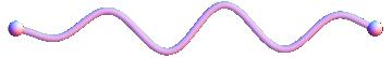
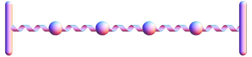
Figure 2. Equivalence among a continuum and a discrete system

Let us consider the diagonal matrix $D^{-1}:=\mathrm{diag}(\frac{1}{\sqrt{m_{1}}},\dots,\frac{1}{\sqrt{m_{N}}})$. Clearly we have that $M=D^{2}$, therefore, by setting

(53) $$u=D^{-1}y,$$

we have that (50) becomes

(54) $$\tilde{L}(y,\dot{y})=L(u,\dot{u})=\frac{1}{2}\sum_{k=1}^{N}\dot{y}_{k}^{2}-\frac{1}{2}y^{\top}D^{-1}KD^{-1}y.$$

If moreover we consider the orthogonal matrix $U$ of the normalized eigenvectors of $D^{-1}KD^{-1}$, by setting

(55) $$y=Uq,$$

the Lagrangian function (50) is represented by

(56) $$\tilde{\tilde{L}}(q,\dot{q})=L(u,\dot{u})=\frac{1}{2}\sum_{k=1}^{N}\dot{q}_{k}^{2}-\frac{1}{2}q^{\top}\tilde{\Lambda}q,$$

where the diagonal matrix $\tilde{\Lambda}:=\mathrm{diag}(\tilde{\lambda}_{1},\dots,\tilde{\lambda}_{N})$ contains the eigenvalues of $D^{-1}KD^{-1}$.

Therefore, the answer to our question is positive if it is possible to choose masses $m_{1},\dots,m_{N}$ and springs $k_{1},\dots,k_{N+1}$ such that the proper frequencies $\tilde{\lambda}_{1},\dots,\tilde{\lambda}_{N}$ coincide with the sequence $\lambda_{1},\dots,\lambda_{N}$ in (37).

This problem is an inverse eigenvalue problem, and has a unique solution in the form of a persymmetric system, i.e., a chain of masses and springs symmetric with respect to the mid point .

Theorem 3.

For any sequence of non negative distinct numbers $0\leqslant\lambda_{1}<\lambda_{2}<\dots<\lambda_{N}$, there exists a unique persymmetric mass–spring system (49-50), $m_{1},\dots,m_{N}$, $k_{1},\dots,k_{N+1}$, with specified total mass $m=\sum_{k=1}^{N}m_{k}$, having the sequence $\lambda_{1},\dots,\lambda_{N}$ as the set of proper oscillation modes.

Proof.

The lines of the proof follows [41, Chapters 3 and 4]. A Jacobi matrix is a positive semi-definite symmetric tridiagonal matrix with (strictly) negative codiagonal entries. If the elastic constants $k_{1},\dots,k_{N+1}$ are all positive, the stiffness matrix $K$ in (50) is a Jacobi matrix. Moreover, if also the masses $m_{1},\dots,m_{N}$ are all positive, the matrix $D^{-1}KD^{-1}$ is still a Jacobi matrix. The proof is completed by invoking

[41, Theorem 4.3.2]: There is a unique, up to multiplicative constants, persymmetric Jacobi matrix $J$ for any assigned spectrum $\sigma(J)=(\lambda_{j})_{j=1}^{N}$, satisfying $0\leqslant\lambda_{1}<\lambda_{2}<\dots<\lambda_{N}$.

As described in details in [41, Section 4.4-4.6] it is possible to reconstruct uniquely a spring-mass system with specified total mass from such a persymmetric Jacobi matrix $J$. ∎

For instance, if we consider the first five eigenvalues of an elastic string and reconstruct an equivalent persymmetric elastic chain with five beads and total mass 1, we obtain the mechanical system:

(57) masses: $$\left\{\frac{5}{21},\frac{5}{28},\frac{1}{6},\frac{5}{28},\frac{5}{21}\right\},$$

(58) springs: $$\frac{\pi^{2}}{L^{2}}\left\{\frac{25}{42},\frac{15}{14},\frac{5}{4},\frac{5}{4},\frac{15}{14},\frac{25}{42}\right\}.$$

The corresponding normalized eigenvectors of the discrete simulacrum are shown in figure 4(b), along with the first five eigenvectors of the continuous system for comparison (c). The eigenvalues of a chain with equal masses and springs are compared with the eigenvalues of the string in figure 3, for a system with 5 masses and 25 masses. Being the largest eigenvalue of the finite chain less than half the corresponding eigenvalue of the string (52), the reconstructed system will not tend to a homogeneous system but a definite difference among masses and springs is maintained as the system size grows.

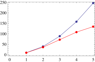
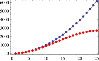
Figure 3. Right panel: first five eigenvalues of the elastic string (blue) and eigenvalues of the elastic chain with five equal masses and springs (red). Left panel: first 25 eigenvalues of the elastic string (blue) and eigenvalues of the elastic chain with 25 equal masses and springs (red).

(a)

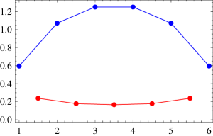
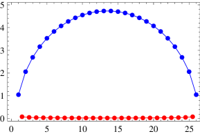
(b)

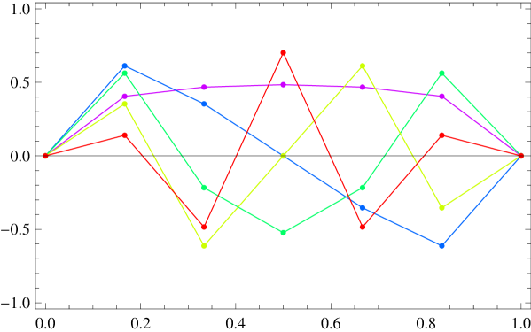
(c)

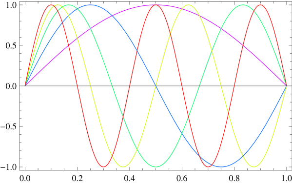
Figure 4. Five-beads elastic chain with the eigenvalues equal to the first five eigenvalues of the elastic string. Panel (a): springs (blue) and masses (red) of the reconstructed system (57-58) with five elements (left) and 25 elements (right). Panel (b): normalized eigenvectors for the chain with 5 elements. Panel (c): first five eigenvectors for the elastic string.

7. Conclusions

The above exploration around the meaning of the exact finite reduction of the PDE setting of a static or dynamic continuous system, here sketched by the problems (1) and (14) respectively, has led us to the following interpretation: such exact reduced system is precisely a discrete ‘simulacrum’ of the original system, reminiscent of all its main features, and it can be perfectly interpreted as a genuine physical system, strictly analogous to the systems of the hierarchy employed in the thermodynamic limit, unless that the masses and springs are not all equal, but persymmetric, i.e., symmetric with respect to the middle point of the system.

References

- [1] Stuart S. Antman. The equations for large vibrations of strings. Amer. Math. Monthly, 87(5):359–370, 1980.
- [2] O. M. Braun and Y. S. Kivshar. The Frenkel-Kontorova model. Texts and Monographs in Physics. Springer-Verlag, Berlin, 2004. Concepts, methods, and applications.
- [3] J. Frenkel and T. Kontorova. On the theory of plastic deformation and twinning. Acad. Sci. U.S.S.R. J. Phys., 1:137–149, 1939.
- [4] N. J. Zabusky and M. D. Kruskal. Interaction of “solitons” in a collisionless plasma and the recurrence of initial states. Phys. Rev. Lett., 15:240–243, Aug 1965.
- [5] D. J. Korteweg and G. de Vries. Xli. on the change of form of long waves advancing in a rectangular canal, and on a new type of long stationary waves. Philosophical Magazine Series 5, 39(240):422–443, 1895.
- [6] John von Neumann. Proposal and Analysis of a New Numerical Method for the Treatment of Hydrodynamical Shock Problems. AMP Report, pages 1–25, March 1944.
- [7] J M Greenberg. Continuum limits of discrete gases. Archive for Rational Mechanics and Analysis, 105(4):367–376, 1989.
- [8] J M Greenberg and Arje Nachman. Continuum limits for discrete gases with long- and short-range interactions. Communications on Pure and Applied Mathematics, 47(9):1239–1281, 1994.
- [9] H. Amann and E. Zehnder. Multiple periodic solutions for a class of nonlinear autonomous wave equations. Houston J. Math., 7(2):147–174, 1981.
- [10] H. Amann and E. Zehnder. Nontrivial solutions for a class of nonresonance problems and applications to nonlinear differential equations. Ann. Scuola Norm. Sup. Pisa Cl. Sci. (4), 7(4):539–603, 1980.
- [11] Herbert Amann. Multiple positive fixed points of asymptotically linear maps. J. Functional Analysis, 17:174–213, 1974.
- [12] Herbert Amann and Eduard Zehnder. Periodic solutions of asymptotically linear Hamiltonian systems. Manuscripta Math., 32(1-2):149–189, 1980.
- [13] Herbert Amann. Saddle points and multiple solutions of differential equations. Math. Z., 169(2):127–166, 1979.
- [14] C. C. Conley and E. Zehnder. The Birkhoff-Lewis fixed point theorem and a conjecture of V. I. Arnol′d. Invent. Math., 73(1):33–49, 1983.
- [15] Charles Conley. Isolated Invariant Sets and The Morse Index. Number 38 in Regional conferences series in mathematics. Conference Board for the Mathematical Sciences, 1976.
- [16] D. Bambusi and S. Paleari. Families of periodic solutions of resonant PDEs. J. Nonlinear Sci., 11(1):69–87, 2001.
- [17] Juha Berkovits, Herbert Leinfelder, and Vesa Mustonen. Existence and multiplicity results for wave equations with time-independent nonlinearity. Topol. Methods Nonlinear Anal., 22(2):273–295, 2003.
- [18] Massimiliano Berti and Philippe Bolle. Multiplicity of periodic solutions of nonlinear wave equations. Nonlinear Anal., 56(7):1011–1046, 2004.
- [19] Massimiliano Berti and Philippe Bolle. Periodic solutions of nonlinear wave equations with general nonlinearities. Comm. Math. Phys., 243(2):315–328, 2003.
- [20] Franco Cardin and Claudio Tebaldi. Finite reductions for dissipative systems and viscous fluid-dynamic models on . J. Math. Anal. Appl., 345(1):213–222, 2008.
- [21] M. Cappiello. Pseudodifferential parametrices of infinite order for SG-hyperbolic problems. Rend. Sem. Mat. Univ. Politec. Torino, 61(4):411–441 (2004), 2003.
- [22] Jean-Michel Coron. Résolution de l’équation où est linéaire autoadjoint et est un opérateur potentiel non linéaire. C. R. Acad. Sci. Paris Sér. A-B, 288(17):A805–A808, 1979.
- [23] Jean-Michel Coron. Résolution de l’équation où est linéaire et dérivé d’un potentiel convexe. Ann. Fac. Sci. Toulouse Math. (5), 1(3):215–234, 1979.
- [24] Marco Degiovanni. On Morse theory for continuous functionals. Conf. Semin. Mat. Univ. Bari, (290):1–22, 2003.
- [25] Rafael de la Llave. Variational methods for quasi-periodic solutions of partial differential equations. In Hamiltonian systems and celestial mechanics (Pátzcuaro, 1998), volume 6 of World Sci. Monogr. Ser. Math., pages 214–228. World Sci. Publ., River Edge, NJ, 2000.
- [26] Alberto Lovison. Generating functions and finite parameter reductions in fields theory. Bollettino Della Unione Matematica Italiana, 8A(3):569–572, DEC 2005.
- [27] Marcello Lucia, Paola Magrone, and Huan-Song Zhou. A Dirichlet problem with asymptotically linear and changing sign nonlinearity. Rev. Mat. Complut., 16(2):465–481, 2003.
- [28] Giovanni Mancini. Periodic solutions of some semilinear autonomous wave equations. Boll. Un. Mat. Ital. B (5), 15(2):649–672, 1978.
- [29] L. Nirenberg. Variational and topological methods in nonlinear problems. Bull. Amer. Math. Soc. (N.S.), 4(3):267–302, 1981.
- [30] Paul H. Rabinowitz. Free vibrations for a semilinear wave equation. Comm. Pure Appl. Math., 31(1):31–68, 1978.
- [31] Sławomir Rybicki. Periodic solutions of vibrating strings. Degree theory approach. Ann. Mat. Pura Appl. (4), 179:197–214, 2001.
- [32] Claude Viterbo. Recent progress in periodic orbits of autonomous Hamiltonian systems and applications to symplectic geometry. In Nonlinear functional analysis (Newark, NJ, 1987), volume 121 of Lecture Notes in Pure and Appl. Math., pages 227–250. Dekker, New York, 1990.
- [33] Claude Viterbo. Symplectic topology as the geometry of generating functions. Mathematische Annalen, 292:685–710, 1992. 10.1007/BF01444643.
- [34] Antonio Di Carlo. private communication.
- [35] C. Boldrighini, A. De Masi, A. Pellegrinotti, and E. Presutti. Collective phenomena in interacting particle systems. Stochastic Process. Appl., 25(1):137–152, 1987.
- [36] Luca Maragliano, Alexander Fischer, Eric Vanden-Eijnden, and Giovanni Ciccotti. String method in collective variables: Minimum free energy paths and isocommittor surfaces. Journal of Chemical Physics, 125(2), JUL 14 2006.
- [37] I. R. Yukhnovskiĭ. Phase transitions of the second order. World Scientific Publishing Co., Singapore, 1987. Collective variables method, Translated from the Russian by A. Y. Saban and S. N. Voitiuk.
- [38] Alessandro Arsie and Christian Ebenbauer. Locating omega-limit sets using height functions. Journal of Differential Equations, 248(10):2458–2469, 2010.
- [39] D Boley and G H Golub. A survey of matrix inverse eigenvalue problems. Inverse Problems, 3(4):595, 1987.
- [40] Christian Ebenbauer and Alessandro Arsie. On an eigenflow equation and its Lie algebraic generalization. Communications in Information and Systems, 8(2):147–170, 2008.
- [41] Graham M. L. Gladwell. Inverse problems in vibration, volume 119 of Solid Mechanics and its Applications. Kluwer Academic Publishers, Dordrecht, second edition, 2004.
- [42] G M L Gladwell. Minimal mass solutions to inverse eigenvalue problems. Inverse Problems, 22(2):539, 2006.
- [43] Xingzhi Ji. On matrix inverse eigenvalue problems. Inverse Problems, 14(2):275, 1998.
- [44] Peter Nylen and Frank Uhlig. Inverse eigenvalue problem: existence of special spring - mass systems. Inverse Problems, 13(4):1071, 1997.
- [45] Ying-Hong Xu and Er-Xiong Jiang. An inverse eigenvalue problem for periodic jacobi matrices. Inverse Problems, 23(1):165, 2007.
- [46] Franco Cardin. Global finite generating functions for field theory. In Classical and quantum integrability (Warsaw, 2001), volume 59 of Banach Center Publ., pages 133–142. Polish Acad. Sci., Warsaw, 2003.
- [47] Franco Cardin, Alberto Lovison, and Mario Putti. Implementation of an exact finite reduction scheme for steady-state reaction-diffusion equations. Internat. J. Numer. Methods Engrg., 69(9):1804–1818, 2007.
- [48] Franco Cardin and Alberto Lovison. Microscopic structures from reduction of continuum nonlinear problems. AAPP — Physical, Mathematical, and Natural Sciences, 91(S1), 2013.
- [49] Antonio Ambrosetti. Critical points and nonlinear variational problems. Mém. Soc. Math. France (N.S.), (49):139, 1992.
- [50] M. M. Vainberg. Variational methods for the study of nonlinear operators. Holden-Day Inc., San Francisco, Calif., 1964. With a chapter on Newton’s method by L. V. Kantorovich and G. P. Akilov. Translated and supplemented by Amiel Feinstein.
- [51] V. Volterra. Leçons sur les Fonctions de Ligne. Gauthier-Villars, Paris, 1913.
- [52] Zhi Qiang Wang. Multiple periodic solutions for a class of nonlinear nonautonomous wave equations. Acta Math. Sinica (N.S.), 5(3):197–213, 1989. A Chinese summary appears in Acta Math. Scinica 33 (1990), no. 4, 575.
- [53] Massimiliano Berti and Philippe Bolle. Sobolev periodic solutions of nonlinear wave equations in higher spatial dimensions. Arch. Ration. Mech. Anal., 195(2):609–642, 2010.
- [54] J. Bourgain. Construction of periodic solutions of nonlinear wave equations in higher dimension. Geom. Funct. Anal., 5(4):629–639, 1995.
- [55] Alberto Lovison, Franco Cardin, and Alessia Bobbo. Discrete structures equivalent to nonlinear dirichlet and wave equations. Continuum Mech Therm, 21(1):27–40, Jan 2009.