Tidal interactions in multi-planet systems

Abstract

We study systems of close orbiting planets evolving under the influence of tidal circularization. It is supposed that a commensurability forms through the action of disk induced migration and orbital circularization. After the system enters an inner cavity or the disk disperses the evolution continues under the influence of tides due to the central star which induce orbital circularization. We derive approximate analytic models that describe the evolution away from a general first order resonance that results from tidal circularization in a two planet system and which can be shown to be a direct consequence of the conservation of energy and angular momentum. We consider the situation when the system is initially very close to resonance and also when the system is between resonances. We also perform numerical simulations which confirm these models and then apply them to two and four planet systems chosen to have parameters related to the GJ581 and HD10180 systems. We also estimate the tidal dissipation rates through effective quality factors that could result in evolution to observed period ratios within the lifetimes of the systems. Thus the survival of, or degree of departure from, close commensurabilities in observed systems may be indicative of the effectiveness of tidal disipation, a feature which in turn may be related to the internal structure of the planets involved.

1 Introduction

Planetary systems containing hot Neptunes and hot super–Earths have been observed recently. A system of this kind consists of the four planets around the M–dwarf GJ 581 (Bonfils et al. 2005, Udry et al. 2007, Mayor et al. 2009a). The projected masses of the planets are 1.9, 15.6, 5.4 and 7.1 M_⊕ and the periods are 3.15, 5.37, 12.93 and 66.8 days, respectively. Other such multiple systems are that around HD 40307 (Mayor et al. 2009b) which consists of three planets with projected masses of 4.2, 6.9 and 9.1 M_⊕ and periods of 4.31, 9.62 and 20.46 days, respectively and that around HD 10180 (Lovis et al. 2010) which consists of seven planets with projected masses 1.35, 13.10, 11.75, 25.1, 23.9, 21.4 and 64.4 M_⊕ and periods of 1.18, 5.76, 16.36, 49.74, 122.76, 601.2, and 2222 days respectively. The innermost member of the latter system has yet to be confirmed.

Migration due to tidal interaction with the disk is a possible mechanism through which planets end up on short period orbits, as in situ formation implies very massive discs (e.g., Raymond et al. 2008). Terquem & Papaloizou 2007 (see also Brunini & Cionco 2005) proposed a scenario for forming hot super–Earths in which a population of cores that formed at some distance from the central star migrated inwards due to interaction with the disk. These collided and merged as they went . This process could produce systems of planets with masses in the earth mass range, located inside an assumed disk inner edge, on short period orbits with mean motions of neighbouring planets that frequently exhibited near commensurabilities. However, tidal circularization of the orbits induced by tidal interaction with the central star, together with later close scatterings and mergers tended to cause the system to move away from earlier established commensurabilities to an extent determined by the effectiveness of these processes.

Papaloizou & Terquem (2010) considered the system around HD 40307 for which the pairs consisting of the innermost and middle planets and the middle and outermost planets are near but not very close to a pair of 2:1 resonances. In spite of this it was found that secular effects produced by the action of the resonant angles coupled with the action of tides from the central star could cause the system to increasingly separate from commensurability. Resonant effects can arise even when departures from strict commensurability are apparently large because tidal circularization produces small eccentricities which, for first order resonances, can be consistent with resonant angle libration (see Murray & Dermott 1999).

In this paper we undertake a further study of systems of close orbiting planets evolving under the influence of tidal circularization. We present simple analytic models describing the evolution away from a general first order resonance for a two planet system under the influence of tidal circularization, describing the situation both when the commensurabilty is very close and also when the system is between resonances. We also perform numerical simulations of two and four planet systems chosen to have parameters related to the GJ581 and HD10180 systems . We consider the situation when various commensurabilities result through the action of assumed disk induced migration and orbital circularization rates, estimating the magnitudes of tidal quality factors that could produce evolution to observed period ratios within the lifetimes of the systems.

The plan of this paper is as follows. In section2.1 we consider a coplanar system of planets in near circular orbits in which orbital energy is dissipated while its total angular momentum is conserved. The system is expected to spread in a similar manner to a viscous accretion disk (see Lynden-Bell & Pringle 1974). For a two planet system, this radial spreading will always lead to evolution away from an initially close commensurability.

In sections 2.2, 2.3 and 3, we carry out an anlaytic study of two planets near to a first order commensurability under the influence of tidal circularization. For planets in the mass range we consider, it is readily estimated that tides raised on the planet are very much more important than tides raised on the star (eg. Goldreich & Soter 1966, Barnes et al. 2009). In addition the orbital decay timescale due to tides raised on the star may be estimated to be much longer than any timescale of interest (eg. Barnes et al. 2009). Thus tides raised on the star have been neglected.

We consider the initial evolution away from a close first order commensurability in section 3.1 and go on to consider the case of evolution when the commensurability is not so close, or the system is between commensurabilities in section 3.2 . As expected from the simple arguments given in section 2.1, the system departs from an initially close commensurability moving to a neighbouring one.

We go on to perform numerical simulations of multiplanet systems in section 4. Various commensurabilities between pairs of planets are set up by applying dissipative forces assumed to arise from a disk, that lead to orbital migration and circularization. These forces were then removed corresponding to assumptions of either entry into an inner cavity or removal of the disk. The evolution of the system under tidal circularization caused by interaction with the central star was then followed. For illustrative purposes we consider two planet systems with parameters corresponding to the two innermost planets in the GJ581 system. In section 4.5 we consider a system that formed a 3:2 commensurability which then evolved under orbital circularization indicating that the model system could attain the period ratio appropriate to the actual system if the tidal parameter $Q^{\prime}$ introduced by Goldreich & Soter (1966) $\sim 100.$ The situation when the system began with disk parameters that led to a 5:3 commensurability is then similarly studied in section 4.6. We go on to consider the effect of adding the additional planets in the GJ581 system in section 4.7.

As there are examples of low mass planetary systems such as HD 10180 which have separations of pairs of planets, the third and fourth innermost in that case, that indicate there may have been a past proximity to a 3:1 commensurability, we consider an exploratory simulation of a system for which the initial disk evolution sets up a 3:1 commensurability in section 4.8. Finally in section 5 we summarize and discuss our results.

2 Commensurabilities and tidal circularization in planetary systems

We begin by considering the evolution of planetary systems undergoing tidal circularization in a general way and then move on to consider simple analytic models of two planet systems that can be close to first order commensurabilities.

2.1 Two interacting planets in circular orbits for which energy is dissipated at fixed total angular momentum

Consider two interacting planets with orbital energies $E_{1}$ and $E_{2}$ respectively. The associated orbital angular momenta for assumed circular orbits are $-2E_{1}/n_{1}$ and $-2E_{2}/n_{2}$ respectively. Here $n_{1}$ and $n_{2}$ are the mean motions associated with the two planets. Suppose now the system dissipates energy while conserving its total angular momentum. This is expected to be the case during orbital circularization when this occurs as a result of stellar tides dissipated in the planets because the planets themselves cannot contain a significant amount of angular momentum. Accordingly we write

$$\frac{dE_{1}}{dt}+\frac{dE_{2}}{dt} = -{\cal{L}},$$ (1)

where ${\cal{L}}$ is the rate of energy dissipation. Angular momentum conservation implies that

$$\frac{1}{n_{1}}\frac{dE_{1}}{dt} = -\frac{1}{n_{2}}\frac{dE_{2}}{dt}$$ (2)

from which we obtain

$$\frac{dE_{1}}{dt} = -\frac{{\cal{L}}}{1-n_{2}/n_{1}},$$ (3)

and

$$\frac{dE_{2}}{dt} = -\frac{{\cal{L}}}{1-n_{1}/n_{2}}.$$ (4)

Supposing that $n_{1}>n_{2},$ the above two equations imply that planet $1$ moves inwards losing energy while planet $2$ moves outwards, taking up the angular momentum lost by planet $1.$ This is the generic form for the evolution of an accretion disc (see Lynden-Bell & Pringle 1974).

We now go on to discuss some simplified models for the interaction of two planets that may be either very close to or some distance away from a strict first order commensurability. In these contexts we show how tidal dissipation induced by forced eccentrcities causes the system to separate. When the resonance is close, this causes the system to depart further from commensurability.

2.2 Coordinate system

We consider a general system of $N$ planets orbiting a central mass. We adopt Jacobi coordinates (Sinclair 1975, Papaloizou & Szuszkiewicz 2005) for which the radius vector of planet $i,$ ${\bf r}_{i},$ is measured relative to the centre of mass of the system comprised of a dominant central mass $M$ and all other planets interior to $i,$ for $i=1,2...,N.$ The planets are assumed to maintain an ordering with increasing $i$ corresponding to greater distances $|{\bf r}_{i}|$ from the dominant central mass. Thus the innermost planet has $i=1.$ The Hamiltonian, correct to second order in the planetary masses, can be written in the form:

$$H = \sum_{i=1}^{N}\left({1\over 2}m_{i}|\dot{\bf r}_{i}|^{2}-{GM_{i}m_{i}\over|{\bf r}_{i}|}\right)$$ (5)

$$- \sum_{i=1}^{N-1}\sum_{j=i+1}^{N}Gm_{i}m_{j}\left({1\over|{\bf r}_{ij}|}-{{\bf r}_{i}\cdot{\bf r}_{j}\over|{\bf r}_{j}|^{3}}\right).$$

Here $M_{i}=M+m_{i}$ and ${\bf r}_{ij}={\bf r}_{i}-{\bf r}_{j}.$

The equations of motion for motion for planet $i$ assumed to move in a fixed plane, about a dominant central mass, may be written in the form (see, e.g., Papaloizou 2003, Papaloizou & Szuszkiewicz 2005):

$$\dot{E}_{i} = -n_{i}\frac{\partial H}{\partial\lambda_{i}}$$ (6)

$$\dot{L}_{i} = -\left(\frac{\partial H}{\partial\lambda_{i}}+\frac{\partial H}{\partial\varpi_{i}}\right)$$ (7)

$$\dot{\lambda}_{i} = \frac{\partial H}{\partial L_{i}}+n_{i}\frac{\partial H}{\partial E_{i}}$$ (8)

$$\dot{\varpi}_{i} = \frac{\partial H}{\partial L_{i}}.$$ (9)

Here the orbital angular momentum of planet $i$ which has reduced mass $m_{i}=m_{i0}M/(M+m_{i0}),$ with $m_{i0}$ being the actual mass, is $L_{i}$ and the orbital energy is $E_{i}.$ For motion around a central point mass $M$ we have:

$$L_{i} = m_{i}\sqrt{GM_{i}a_{i}(1-e_{i}^{2})},$$ (10)

$$E_{i} = -{{GM_{i}m_{i}}\over{2a_{i}}},$$ (11)

where $M_{i}=M+m_{i0},$ $a_{i}$ denotes the semi-major axis and $e_{i}$ the eccentricity of planet $i.$

The mean longitude of planet $i$ is $\lambda_{i}=n_{i}(t-t_{0i})+\varpi_{i},$ where $n_{i}=\sqrt{GM_{i}/a_{i}^{3}}$ is its mean motion, with $t_{0i}$ denoting its time of periastron passage and $\varpi_{i}$ the longitude of periastron.

From equations (6) and (7) an equation for the evolution of the eccentricity of planet $i$ may be readily obtained in the form

$$\dot{e}_{i} = \frac{\sqrt{1-e_{i}^{2}}}{e_{i}m_{i}n_{i}a_{i}^{2}}\left(\frac{\partial H}{\partial\lambda_{i}}\left(\sqrt{1-e_{i}^{2}}-1\right)+\frac{\partial H}{\partial\varpi_{i}}\right).$$ (12)

The Hamiltonian may be expanded in a Fourier series involving linear combinations of the $(2N-1)$ angular differences $\varpi_{i}-\varpi_{1},i=2,3..N$ and $\lambda_{i}-\varpi_{i},i=1,2,..N.$ In the limit of small eccentricities of interest here, only terms that are of first order in the eccentricities need to be retained (terms that are of zero order do not lead to changes to eccentricities or to resonances). If this is done the possibility of first order resonances, for which the ratio of the periods of two planets is the ratio of successive integers, is allowed for. The above approximation scheme should be valid when circularization times are small enough to ensure that the eccentricities remain small. This situation is realized for examples of low mass protoplanets migrating in protoplanetary discs (Papaloizou & Szuszkiewicz 2005).

Near a first order $p+1:p$ resonance, $p$ being an integer, we expect that terms in the Hamiltonian involving angles of the type $\phi_{p,j,i,j}=(p+1)\lambda_{j}-p\lambda_{i}-\varpi_{j},$ and $\phi_{p,j,i,i}=(p+1)\lambda_{j}-p\lambda_{i}-\varpi_{i},$ where the subscripts on the left hand side correspond to those on the right hand reading from left to right, will be slowly varying and thus be dominant. Accordingly we shall retain only terms of this type. Motion away from resonances may also be considered having made this approximation although neglected high frequency modulations may be more significant then.

The Hamiltonian may be written in the form

$$H=\sum_{i=1}^{N}E_{i}+\sum_{i=1}^{N-1}\sum_{j=i+1}^{N}H_{i,j},$$ (13)

where the component of the interaction Hamiltonian $H_{i,j}$ that is first order in the eccentricities is given, given that $j>i,$ by

$$H_{i,j}=-\frac{Gm_{i}m_{j}}{a_{j}}\sum_{p=1}^{\infty}\left(e_{j}C_{p,j,i,j}\cos(\phi_{p,j,i,j})+e_{i}D_{p,j,i,i}\cos(\phi_{p,j,i,i})\right),$$ (14)

with

$$C_{p,j,i,j}={1\over 2}\left(x{d(b^{(p)}_{1/2}(x))\over dx}+(2p+1)b^{(p)}_{1/2}(x)-4x\delta^{p}_{1}\right)\ \ {\rm and}\ \$$ (15)

$$D_{p,j,i,i}=-{1\over 2}\left(x{d(b^{(p+1)}_{1/2}(x))\over dx}+2(p+1)b^{(p+1)}_{1/2}(x)\right).$$ (16)

Here $b^{(p)}_{1/2}(x)$ denotes the usual Laplace coefficient (e.g. Brouwer & Clemence 1961) with the argument $x=a_{i}/a_{j}$ and $\delta^{p}_{1}$ denotes the Kronnecker delta. We remark that the subscripts associated with the coefficients $C_{p,j,i,j}$ and $D_{p,j,i,i}$ correspond to the related angles as in (14). We shall also make the approximation of replacing $M_{i}$ by $M$ and equivalently $m_{i0}$ by $m_{i}.$

The governing equations for motion, retaining only terms that are of the lowest order in the eccentricities, follow from Hamilton’s equations (6)- (9) for the Hamiltonian (13) discussed above as

$$\frac{de_{i}}{dt} = -\sum_{p=1}^{\infty}\left[\sum_{j=i+1}^{N}\frac{Gm_{j}D_{p,j,i,i}\sin(\phi_{p,j,i,i})}{n_{i}a_{i}^{2}a_{j}}+\sum_{j=1}^{i-1}\frac{Gm_{j}C_{p,i,j,i}\sin(\phi_{p,i,j,i})}{n_{i}a_{i}^{3}}\right]$$ (17)

$$\frac{dn_{i}}{dt} = -\sum_{p=1}^{\infty}\left[\sum_{j=i+1}^{N}\frac{3Gm_{j}p}{a_{i}^{2}}\left(\frac{e_{i}D_{p,j,i,i}\sin(\phi_{p,j,i,i})}{a_{j}}+\frac{e_{j}C_{p,j,i,j}\sin(\phi_{p,j,i,j})}{a_{j}}\right)\right.$$ (18)

$$- \left.\sum_{j=1}^{i-1}\frac{3Gm_{j}(p+1)}{a_{i}^{2}}\left(\frac{e_{j}D_{p,i,j,j}\sin(\phi_{p,i,j,j})}{a_{i}}+\frac{e_{i}C_{p,i,j,i}\sin(\phi_{p,i,j,i})}{a_{i}}\right)\right]$$

$$\frac{d\varpi_{i}}{dt} = \sum_{p=1}^{\infty}\left[\sum_{j=i+1}^{N}\frac{Gm_{j}D_{p,j,i,i}\cos(\phi_{p,j,i,i})}{e_{i}n_{i}a_{i}^{2}a_{j}}+\sum_{j=1}^{i-1}\frac{Gm_{j}C_{p,i,j,i}\cos(\phi_{p,i,j,i})}{e_{i}n_{i}a_{i}^{3}}\right].$$ (19)

In addition, consistent with the above approximation scheme, the rate of change of the mean longitudes may be obtained from

$$\frac{d\lambda_{i}}{dt}=n_{i}$$ (20)

which also enables evaluation of the rate of change of the angles $\phi_{p,j,i,i},\phi_{p,j,i,j}$ etc.

2.3 The incorporation of disk tides

We incorporate the effects of orbital circularization by adding additional terms to the right hand sides of equations (17) and (18). Equation (17) is modified through the straightforward prescription

$$\frac{de_{i}}{dt}\rightarrow\frac{de_{i}}{dt}-\frac{e_{i}}{t_{c,i}},$$ (21)

where $t_{c,i}$ is the circularization time for planet $i.$ Similarly equation (18) is modified according to

$$\frac{dn_{i}}{dt}\rightarrow\frac{dn_{i}}{dt}+\frac{3n_{i}e_{i}^{2}}{t_{c,i}}.$$ (22)

This adjustment is necessary to account for the orbital energy dissipation occurring as a result of circularization correct to the lowest order in $e_{i}.$ This dissipation is assumed to occur with out changing the angular momentum of the system because the planets can only potentially contain a negligible amount of angular momentum compared to that in the orbit. It follows from the energy dissipation rate for planet, $i,$ given by

$$\frac{dE_{i}}{dt}=-\frac{m_{i}n_{i}^{2}a_{i}^{2}e_{i}^{2}}{(1-e^{2}_{i})t_{c,i}}.$$ (23)

For small eccentricities, $e_{i}^{2}$ may be neglected in the denominator of the above expression and the total rate of energy dissipation in the system is obtained by summing over all planets.

3 Two planets in a $p+1:p$ commensurability

It is possible to investigate solutions of equations (17) - (19) modified to incorporate circularization, that illustrate the geometrical separation of the system as energy is dissipated while the total angular momentum is conserved, in a number circumstances.

3.1 A tight commensurability

We begin with an example where two successive planets $k$ and $k+1$ maintain a $p+1:p$ commensurability with the associated angles in a state of at most small amplitude libration while their semi-major axes separate. We later go on to consider a simple restricted example where the angle circulates. The effects of planets other than the resonant pair is neglected. Equations(17) - (19) with the modifications given by (21) and (22) to incorporate circularization give the governing equations for planet $k$ in the form

$$\frac{de_{k}}{dt} = -\frac{Gm_{k+1}D_{p,k+1,k,k}\sin(\phi_{p,k+1,k,k})}{n_{k}a_{k}^{2}a_{k+1}}-\frac{e_{k}}{t_{c,k}}$$ (24)

$$\frac{dn_{k}}{dt} = -\frac{3Gm_{k+1}p}{a_{k}^{2}}\left(\frac{e_{k}D_{p,k+1,k,k}\sin(\phi_{p,k+1,k,k})}{a_{k+1}}\right.$$ (25)

$$+ \left.\frac{e_{k+1}C_{p,k+1,k,k+1}\sin(\phi_{p,k+1,k,k+1})}{a_{k+1}}\right)+\frac{3n_{k}e_{k}^{2}}{t_{c,k}}$$

$$\frac{d\varpi_{k}}{dt} = \frac{Gm_{k+1}D_{p,k+1,k,k}\cos(\phi_{p,k+1,k,k})}{e_{k}n_{k}a_{k}^{2}a_{k+1}}.$$ (26)

Similarly the governing equations for planet $k+1$ are given by

$$\frac{de_{k+1}}{dt} = -\frac{Gm_{k}C_{p,k+1,k,k+1}\sin(\phi_{p,k+1,k,k+1})}{n_{k+1}a_{k+1}^{3}}-\frac{e_{k+1}}{t_{c,k+1}}$$ (27)

$$\frac{dn_{k+1}}{dt} = \frac{3Gm_{k}(p+1)}{a_{k+1}^{2}}\left(\frac{e_{k}D_{p,k+1,k,k}\sin(\phi_{p,k+1,k,k})}{a_{k+1}}\right.$$ (28)

$$+ \left.\frac{e_{k+1}C_{p,k+1,k,k+1}\sin(\phi_{p,k+1,k,k+1})}{a_{k+1}}\right)+\frac{3n_{k+1}e_{k+1}^{2}}{t_{c,{k+1}}}$$

$$\frac{d\varpi_{k+1}}{dt} = \frac{Gm_{k}C_{p,k+1,k,k+1}\cos(\phi_{p,k+1,k,k+1})}{e_{k+1}n_{k+1}a_{k+1}^{3}}.$$ (29)

Setting $\phi_{p,k+1,k,k}\rightarrow\phi_{p,k+1,k,k}\pm\Delta\phi_{p,k+1,k,k}$ and $\phi_{p,k+1,k,k+1}\rightarrow\phi_{p,k+1,k,k+1}\pm\Delta\phi_{p,k+1,k,k+1},$ where the positive sign is taken when the equilibrium value of the angle is zero and the negative sign is taken when it is $\pi,$ and $\Delta$ indicates a small shift such that the sines of the angles may be replaced by the angles themselves. Then assuming that the evolutionary time scale is much longer than the circularization times so that the time derivatives of the eccentricities may be neglected, we can then find expressions for the small angular shifts in the form

$$\Delta\phi_{p,k+1,k,k} = -\frac{e_{k}n_{k}a_{k}^{2}a_{k+1}}{Gm_{k+1}D_{p,k+1,k,k}t_{c,k}}.$$ (30)

$$\Delta\phi_{p,k+1,k,k+1} = -\frac{e_{k+1}n_{k+1}a_{k+1}^{3}}{Gm_{k}C_{p,k+1,k,k+1}t_{c,k+1}}.$$ (31)

Substituting these into the equations for the evolution of the mean motions yields

$$\frac{dn_{k}}{dt} = \frac{3(p+1)e_{k}^{2}n_{k}}{t_{c,k}}+\frac{3pm_{k+1}e_{k+1}^{2}n_{k+1}a_{k+1}^{2}}{m_{k}a_{k}^{2}t_{c,k+1}}$$ (32)

$$\frac{dn_{k+1}}{dt} = -\frac{3(p+1)m_{k}e_{k}^{2}n_{k}a_{k}^{2}}{m_{k+1}t_{c,k}a_{k+1}^{2}}-\frac{3pe_{k+1}^{2}n_{k+1}}{t_{c,k+1}}.$$ (33)

The above pair of equations express the conservation of energy and angular momentum for the system in the limit of small eccentricity. We remark that the latter follows in the form

$$m_{k+1}a_{k+1}^{2}\frac{dn_{k+1}}{dt}+m_{k}a_{k}^{2}\frac{dn_{k}}{dt}=0,$$ (34)

while the former follows from using the fact that $E_{j}\propto m_{j}n_{j}^{2/3}$ to find equations for $dE_{j}/dt,j=k,k+1$ and then adding. We may also obtain an equation showing how the period ratio increases with time in the form

$$\frac{d}{dt}\left(\frac{n_{k}}{n_{k+1}}\right)=\frac{3n_{k}J}{n_{k+1}}\left[\frac{(p+1)e_{k}^{2}}{t_{c,k}J_{k+1}}+\frac{pe_{k+1}^{2}}{t_{c,k+1}J_{k}}\right],$$ (35)

where $J_{k}=m_{k}a_{k}^{2}n_{k},$ and $J=J_{k}+J_{k+1}.$ In order to proceed further we need to calculate the eccentricities. These may be obtained from the governing equations for the evolution of the angles that may be obtained from (20), (26) and (29) in the form

$$\frac{d\phi_{p,k+1,k,k}}{dt} = (p+1)n_{k+1}-pn_{k}-\frac{Gm_{k+1}D_{p,k+1,k,k}\cos(\phi_{p,k+1,k,k})}{e_{k}n_{k}a_{k}^{2}a_{k+1}}.$$ (36)

$$\frac{d\phi_{p,k+1,k,k+1}}{dt} = (p+1)n_{k+1}-pn_{k}-\frac{Gm_{k}C_{p,k+1,k,k+1}\cos(\phi_{p,k+1,k,k+1})}{e_{k+1}n_{k+1}a_{k+1}^{3}}.$$ (37)

As the angles are quasi-steady and close to zero or $\pi,$ these expressions enable the calculation of the squares of the eccentricities $e_{k}$ and $e_{k+1}$ which are required in order to calculate the rate of period separation through (35). They are found to be given by

$$e_{k}^{2} = \left(\frac{Gm_{k+1}D_{p,k+1,k,k}}{n_{k}a_{k}^{2}a_{k+1}[(p+1)n_{k+1}-pn_{k}]}\right)^{2}\hskip 28.45274pt{\rm and}$$ (38)

$$e_{k+1}^{2} = \left(\frac{Gm_{k}C_{p,k+1,k,k+1}}{n_{k+1}a_{k+1}^{3}[(p+1)n_{k+1}-pn_{k}]}\right)^{2}\hskip 28.45274pt{\rm respectively}.$$ (39)

Using these in (35) we obtain

$$\frac{d}{dt}\left(\frac{n_{k}}{n_{k+1}}-\frac{p+1}{p}\right)^{3}=\frac{9n_{k}J}{n_{k+1}}F,$$ (40)

where

$$F=\frac{(p+1)}{t_{c,k}J_{k+1}}\left(\frac{Gm_{k+1}D_{p,k+1,k,k}}{pn_{k}n_{k+1}a_{k}^{2}a_{k+1}}\right)^{2}+\frac{p}{t_{c,k+1}J_{k}}\left(\frac{Gm_{k}C_{p,k+1,k,k+1}}{pn_{k+1}^{2}a_{k+1}^{3}}\right)^{2}.$$ (41)

When the system starts to move away from a commensurability taken to be exact at $t=0,$ we may treat the right hand side of (40) as being constant and integrate with respect to time to obtain

$$\frac{n_{k}}{n_{k+1}}-\frac{p+1}{p}=\left(\frac{9n_{k}J}{n_{k+1}}Ft\right)^{1/3}.$$ (42)

A similar scaling for which the separation from a commensurability increases $\propto t^{1/3}$ was obtained for a three planet system by Papaloizou & Terquem (2010).

3.2 The interaction between two planets away from a close commensurability

In this case we again assume interaction between planets $k$ and $k+1.$ In this case we consider the situation away from a strict commensurability where significant libration or circulation may occur. This is a natural development as tidal evolution causes the system to evolve away from a tight commensurability of the type described above towards such a situation. We make the additional simplification of assuming that $m_{k+1}\gg m_{k}.$ In that case, a circular restricted $3$ body problem may be adopted. Only the motion of planet $k$ is considered with $e_{k+1}=0.$ Equations (17) - (20) apply and as $e_{k+1}=0,$ only terms involving the angles $\phi_{p,k+1,k,k},p=1,2...$ appear. These give the equations governing the evolution as

$$\frac{de_{k}}{dt} = -\frac{e_{k}}{t_{c,k}}-\sum_{p=1}^{\infty}\frac{Gm_{k+1}D_{p,k+1,k,k}\sin(\phi_{p,k+1,k,k})}{n_{k}a_{k}^{2}a_{k+1}}$$ (43)

$$\frac{dn_{k}}{dt} = \frac{3n_{k}e_{k}^{2}}{t_{c,k}}-\sum_{p=1}^{\infty}\frac{3Gm_{k+1}pe_{k}D_{p,k+1,k,k}\sin(\phi_{p,k+1,k,k})}{a_{k+1}a_{k}^{2}}$$ (44)

$$\frac{d\phi_{r,k+1,k,k}}{dt} = (r+1)n_{k+1}-rn_{k}-\sum_{p=1}^{\infty}\frac{Gm_{k+1}D_{p,k+1,k,k}\cos(\phi_{p,k+1,k,k})}{e_{k}n_{k}a_{k}^{2}a_{k+1}},$$

$$r=1,2,3 .\hskip 5.69054pt.$$ . (45)

Although we consider the effect of more than one angle, we focus on a particular one with $r=q$ which might be considered to be the one closest to resonance, though that is not essential. Setting $x=e_{k}\cos(\phi_{q,k+1,k,k})$ and $y=e_{k}\sin(\phi_{q,k+1,k,k})$ in equations (43) and ( 45 ) leads to a system that, unlike the original one, does not contain an apparent singularity as $e_{k}\rightarrow 0$ in the form

$$\frac{dx}{dt} = -\omega_{q}y-\frac{x}{t_{c,k}}-\sum_{p=1\neq q}^{\infty}\alpha_{p}\sin[(p-q)(\lambda_{k+1}-\lambda_{k})]$$ (46)

$$\frac{dy}{dt} = -\alpha_{q}+\omega_{q}x-\frac{y}{t_{c,k}}-\sum_{p=1\neq q}^{\infty}\alpha_{p}\cos[(p-q)(\lambda_{k+1}-\lambda_{k})],$$ (47)

where, recalling that $k$ is fixed, we define $\alpha_{q}=Gm_{k+1}D_{q,k+1,k,k}/(n_{k}a_{k}^{2}a_{k+1})$
and $\omega_{q}=(q+1)n_{k+1}-qn_{k}.$

We now remark that if we consider the limit $e_{k}\rightarrow 0,$ which occurs far enough away from resonance, we may neglect the evolution of $n_{k}$ and asume that it remains constant and equal to $n_{k0}.$ To see this it follows from (43) that $e_{k}$ scales as $m_{k+1}$ while (44) then indicates that the change in $n_{k},$ $\delta n_{k}=n_{k}-n_{k0}$ scales as $m_{k+1}^{2}$ or $e_{k}^{2}.$ Accordingly, for $q$ of order unity, the induced variation of $w_{q},$ $\delta\omega_{q},$ is such that $\delta\omega_{q}\sim n_{k0}e_{k}^{2}.$ By comparing the variation of the first two terms on the right hand side of equation (47), it readily follows in the low eccentricity limit that provided $n_{k0}e_{k}^{3}\ll\alpha_{q}$ or

$$e_{k}\ll\left(\frac{Gm_{k+1}D_{q,k+1,k,k}}{n_{k}^{2}a_{k}^{2}a_{k+1}}\right)^{1/3},$$ (48)

the variation of $n_{k}$ may be neglected so that it may be taken to be equal to $n_{k0}.$ Similarly $a_{k}$ is replaced by the corresponding fixed value $a_{k0}.$ The above approximation scheme applies in the low eccentricity limit or sufficiently far away from strict commensurability such that $|\omega_{q}|=|(q+1)n_{k+1}-qn_{k0}|\gg n_{k0}^{1/3}\alpha_{q}^{2/3}.$

Given that in the same approximation (20) implies that

$\lambda_{k+1}-\lambda_{k}=(n_{k+1}-n_{k0})t,$ equations (46) and (47) describe a linear system with prescribed harmonic forcing that is easily solved exactly. The solution in the limit $t_{c}\rightarrow\infty$ may be written

$$x = x_{0}+\sum_{p=1\neq q}^{\infty}\frac{\alpha_{p}\cos[(p-q)(\lambda_{k+1}-\lambda_{k})]}{(p+1)n_{k+1}-pn_{k}}$$ (49)

$$y = -\sum_{p=1\neq q}^{\infty}\frac{\alpha_{p}\sin[(p-q)(\lambda_{k+1}-\lambda_{k})]}{(p+1)n_{k+1}-pn_{k}},$$ (50)

where $x_{0}=\alpha_{q}/\omega_{q}.$ This indicates oscillation about the mean value of $x=x_{0}.$ In the absence of the periodic forcing circularization would cause the solution to approach $x=x_{0},y=0$ corresponding to a precise commensurability with zero libration amplitude. When the forcing is present, there is either libration or circulation depending on the ratio of the forcing amplitude to $x_{0}.$ When $q+1:q$ is the closest commensurability, this can be small resulting in small amplitude libration. When some other commensurability is dominant, the motion in the $(x,y)$ plane is around an approximately circular curve that encloses the origin and so corresponds to circulation. Thus as the system moves through a commensurabilty the motion is expected to change from circulation to libration to circulation (see Terquem & Papaloizou 2007 for an example of evolution away from a first order commensurability driven by orbital circularization). Note that in all of these cases the time dependent averages of quantities such as $e_{k}\cos(\phi_{q,k+1,k,k})\equiv x$ and $\cos(\phi_{q,k+1,k,k})$ are generally non zero (see also Papaloizou & Terquem 2010).

In order to calculate the rate of energy dissipation resulting from orbital circularization and hence the rate of evolution it causes, we require the time average of the square of the eccentricity. This is given by

$$\langle e_{k}^{2}\rangle=\langle x^{2}+y^{2}\rangle=\sum_{p=1}^{\infty}\frac{\alpha_{p}^{2}}{[(p+1)n_{k+1}-pn_{k}]^{2}}.$$ (51)

We remark that this expression connects to that found for the tight resonance example (38). The latter expression is identical to that given by (51) if only one term is retained that corresponds to the tight commensurability considered. Thus we expect the evolution to continue to be dominated by the closest comensurability until another becomes closer and takes over governing the evolution.

3.3 The orbital evolution of the planet

The rate of change of the orbital energy may be obtained from consideration of (51) and (23) together with the discussion leading to equation (3) given in section 2.1 with the result that

$$\frac{dE_{k}}{dt}\equiv-\frac{m_{k}a_{k}^{2}n_{k}n_{k+1}}{3}\frac{d}{dt}\left(\frac{n_{k}}{n_{k+1}}\right)=-\frac{m_{k}n_{k}^{2}a_{k}^{2}}{(1-n_{k+1}/n_{k})t_{c,k}}\sum_{p=1}^{\infty}\frac{\alpha_{p}^{2}}{[(p+1)n_{k+1}-pn_{k}]^{2}}$$ (52)

which means that the orbit of $m_{k}$ contracts and separates from that of $m_{k+1}.$ In the limit $m_{k}/m_{k+1}\rightarrow 0$ in which $n_{k+1}$ becomes fixed, and close to a commensurability (52) becomes equivalent to (40). Thus it enables the discussion of the situation corresponding to a tight commensurability to be extended to conditions away from close commensurability. In view if the fact that $n_{k}/n_{k+1}$ must always increase, such a discussion leads to the conclusion that the evolution will be controlled by successive first order comensurabilities as the system widens (see also Terquem & Papaloizou 2007).

4 Numerical Simulations

We here describe simulations of model planetary systems in which commensurabilties have been formed subsequently evolving under the influence of circularization tides.

4.1 Model and initial conditions

We consider a primary star together with N planets embedded in a gaseous disk surrounding it. The planets undergo gravitational interaction with each other and the star and are acted on by tidal forces from the disk and star. The system is solved as an $N$–body problem. Tidal interactions are incorporated by applying appropriate dissipative forces (see Terquem & Papaloizou 2007 and Papaloizou & Terquem 2010 for more details and examples). The equations of motion may be written as

$${d^{2}{\bf r}_{i}\over dt^{2}}=-{GM{\bf r}_{i}\over|{\bf r}_{i}|^{3}}-\sum_{j=1\neq i}^{N}{Gm_{j0}\left({\bf r}_{i}-{\bf r}_{j}\right)\over|{\bf r}_{i}-{\bf r}_{j}|^{3}}-{\bf\Gamma}+{\bf\Gamma}_{i}+{\bf\Gamma}_{r}\;,$$ (53)

where $M$, $m_{j0}$ and ${\bf r}_{j}$ denote the mass of the central star, that of planet $j$ and the position vector of planet $j$, respectively. The acceleration of the coordinate system based on the central star (indirect term) is given by

$${\bf\Gamma}=\sum_{j=1}^{N}{Gm_{j0}{\bf r}_{j}\over|{\bf r}_{j}|^{3}},$$ (54)

and that due to tidal interaction with the disk and/or the star is dealt with through the addition of dissipative forces (see Papaloizou & Larwood 2000). Thus

$${\bf\Gamma}_{i}=-\frac{1}{t_{mg,i}}\frac{d{\bf r}_{i}}{dt}-\frac{2}{|{\bf r}_{i}|^{2}t_{e,i}}\left(\frac{d{\bf r}_{i}}{dt}\cdot{\bf r}_{i}\right){\bf r}_{i}-\frac{2}{t_{i,i}}\left(\frac{d{\bf r}_{i}}{dt}\cdot{\bf e}_{z}\right){\bf e}_{z},$$ (55)

where $t_{mg,i}$, $t_{e,i}$ and $t_{i,i}$ are the timescales over which, respectively, the angular momentum, the eccentricity and the inclination with respect to the unit normal ${\bf e}_{z}$ to the assumed fixed gas disk midplane change. Evolution of the angular momentum and inclination is assumed to be due to tidal interaction with the disk, whereas evolution of the eccentricity is assumed to occur due to both tidal interaction with the disk and the star. We have:

$$\frac{1}{t_{e,i}}=\frac{1}{t_{c,i}^{d}}+\frac{1}{t_{c,i}},$$ (56)

where $t_{c,i}^{d}$ and $t_{c,i}$ are the contribution from the disk and tides raised by the star, respectively. Relativistic effects are modeled through ${\bf\Gamma}_{r}$ ( see Papaloizou & Terquem 2001).

Because a low mass planet cannot contain a significant quantity of angular momentum, tides raised on it by interaction with the star are assumed not to modify the angular momentum of the orbit. We remark that the orbital decay timescale, due to tides raised on the star, is readily estimated to be much longer than any timescale of interest (eg. Barnes et al 2009) thus these tides are ignored from now on.

4.2 Orbital circularization due to tides from the central star

The circularization timescale due to tidal interaction with the star, in the small eccentricity limit appropriate here, is taken to be ( Goldreich & Soter 1966)

$$t_{c,i}=4.65\times 10^{4}\;\left(\frac{{\rm M}_{\odot}}{M}\right)^{3/2}\left(\frac{{\rm M}_{\oplus}}{m_{i0}}\right)^{2/3}\left(\frac{20a_{i}}{{\rm 1~{}au}}\right)^{6.5}Q^{\prime}\;\;\;{\rm years},$$ (57)

where $a_{i}$ is the semi–major axis of planet $i.$ Here we have adopted a mass density of 1 g cm³ for the planets (uncertainties in this quantity could be incorporated into a redefinition of $Q^{\prime}$). The parameter $Q^{\prime}=3Q/(2k_{2}),$ where $Q$ is the tidal dissipation function and $k_{2}$ is the Love number. For solar system planets in the terrestrial mass range, Goldreich & Soter (1966) give estimates for $Q$ in the range 10–500 and $k_{2}\sim 0.3$, which correspond to $Q^{\prime}$ in the range 50–2500. We remark that this parameter should be regarded as being very uncertain for extrasolar planets. As computations with increasing $Q^{\prime}$ become prohibitive on account of long evolution times, we have considered values of $Q^{\prime}$ of $1.5$ and $3$ in this paper. However, we have obtained scaling relations which indicate how to scale results to larger $Q^{\prime}.$

4.3 Type I migration

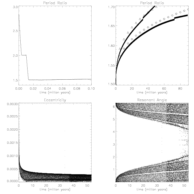
Figure 1: The evolution of two planets that form a 3:2 commensurability. The early evolution of the period ratio during convergent migration is shown in the upper left panel. The upper right panel shows the evolution of the period ratio under orbital circularization after disk migration ceases. The uppermost curve is for $Q^{\prime}=1.5$ and the lower curve is for $Q^{\prime}=3.$ The triangles/diamonds correspond to the analytic predictions made from equation (42) adapted to the case of a 3:2 commensurability for $Q^{\prime}=1.5/Q^{\prime}=3$ respectively. The evolution of the eccentricity of the outermost planet is plotted in the lower left panel for $Q^{\prime}=1.5.$ The evolution of the resonant angle $3\lambda_{2}-2\lambda_{1}-\varpi_{1}$ is plotted in the lower right panel for $Q^{\prime}=1.5.$

When a planet is in contact with the disk, disk–planet interactions occur leading to orbital migration as well as eccentricity and inclination damping (e.g., Ward 1997). However, the migration rates to be used are uncertain even when the disk surface density is known, largely because of uncertainties regarding the effectiveness of coorbital torques (e.g., Paardekooper & Melema 2006, Pardekooper & Papaloizou 2008, 2009). In this context there are indications from modelling the observational data that the adopted type I migration rate should be significantly below that predicted by the linear calculations of Tanaka et al. (2002) (see Schlaufman et al 2009). Hence we have carried out simulations with $t_{mg,i}$ and $t_{e,i}^{d}$ for any system taken, as for type I migration, to be proportional to $1/m_{i}$ and adopted $t_{i,i}=t_{e,i}^{d}.$ A range of scaling constants was explored. These are quoted together with corresponding numerical results below.

We remark that provided that eccentricity damping limits eccentricities to small values, the commensurabilities that are formed in the system as a consequence of convergent migration depend on the ratio of the adopted migration rate to the local orbital frequency, with commensurabilities of low order and low degree forming when this ratio is small.

4.4 Numerical results

4.5 A system with a 3:2 commensurability

For the calculatioas presented in this section we adopted masses for the two planets and the central star that coincided with those for the star and two innermost planets of the GJ581 system. Thus the inner planet was taken to have a mass $m_{1}=1.94M_{\oplus}$ and to be in circular orbit at $0.16au.$ The outer planet was taken to have a mass $m_{i}=15.64M_{oplus}$ and to be in a circular orbit at $0.32au.$ Tests indicate that the results of simulations of the type described here do not depend on the longitudes at which the planets are inserted on such circular orbits. The central mass was $0.31M_{\odot}.$ The initial semi-major axes were chosen to be larger than the corresponding ones in the GJ581 system so as to allow for some inward migration. The disk migration and circularization rates adopted were given by

$$t_{mig}=4.375\times 10^{5}\frac{M_{\oplus}}{m_{i}}yr.\hskip 5.69054pt{\rm and}\hskip 5.69054ptt_{c,i}=5\times 10^{2}\frac{M_{\oplus}}{m_{i}}yr.$$ (58)

However, they were only applied when the semi-major axis of a planet exceeded $0.041au.$ This procedure results in the final semi-major axis of the outer planet to coincide with the second planet in the GJ581 system. The termination of disk migration could be regarded as either being due to entry into an inner cavity, or simply removal of the disk. The migration rate was chosen so as to enable the planets to settle into a 3:2 commensurability through convergent migration. A very much slower rate would allow trapping in a 2:1 commensurability, while a very much faster one would result in the system passing through the 3:2 commensurability (see eg. Papaloizou & Szuskewicz 2010). We remark that although the specific parameters chosen correspond to the GJ581 system, the aruments presented above indicate that the form of evolution we find should be generic for two low mass planets attaining a first order commensurability through convergent migration.

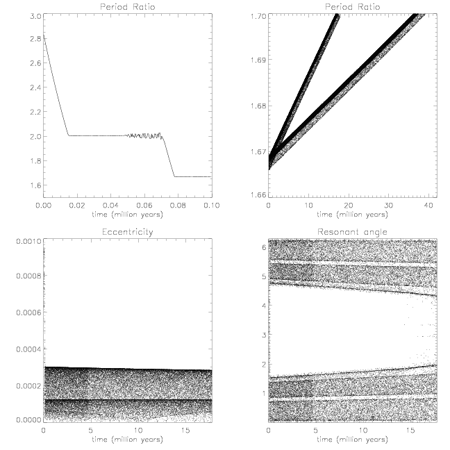
Figure 2: The evolution of two planets that form a 5:3 commensurability. The early evolution of the period ratio during convergent migration is shown in the upper left panel. The upper right panel shows the evolution of the period ratio under orbital circularization after disk migration ceases. The uppermost curve is for $Q^{\prime}=1.5$ and the lower curve is for $Q^{\prime}=3.$ The evolution of the eccentricity of the outermost planet is plotted in the lower left panel. The evolution of the resonant angle $3\lambda_{2}-2\lambda_{1}-\varpi_{1}$ is plotted in the lower right panel.

The evolution of the system is illustrated in Fig. 1. The early evolution of the period ratio during convergent migration is shown in the upper left panel. It is seen that the system is trapped in a 2:1 commensurability for a while before escaping to be subsequently trapped in a 3:2 commensurability. After about $2\times 10^{4}yr.$ the forces from the disk cease to act and the system evolves under tidal circularization. The upper right panel of Fig. 1 shows the evolution of the period ratio. Results for simulations with $Q^{\prime}=1.5$ and $Q^{\prime}=3$ are illustrated and compared to analytic predictions derived from equation (42) adapted to the cases on hand. Interestingly the numerical results are in quite good agreement with what is expected from the analytic discussion given in section 3 which assumed a small libration amplitude and which led to equation (42), even in regimes where the amplitude of libration of the resonant angle is quite large. However, the simulations show additional sudden small jumps in the period ratio which occur when the system passes through the 5:3 resonance. This jump was larger for the $Q^{\prime}=1.5$ case than for the $Q^{\prime}=3$ case. The evolution of the resonant angle $3\lambda_{2}-2\lambda_{1}-\varpi_{1}$ for $Q^{\prime}=1.5.$ shown in Fig. 1 indicates an increasing amplitude libration that tends to break down near the end of the simulation when the period ratio $\sim 1.7$ as in GJ581. But note that there is also a short temporary breakdown as the system passes through 5:3 resonance. Note that the anlaytic treatment suggests the time for the period ratio to evolve from 1.5 to 1.7 to be $\sim 5\times 10^{6}yr.$ The simulation with $Q^{\prime}=1.5.$ rather fortuitously agrees very well with this. The analytic prediction for $Q^{\prime}=3$ is $10^{7}yr.$ while the simulations discussed in this and the next section indicate $1.3\times 10^{7}yr.$ Given the expectation that evolution times are $\propto Q^{\prime},$ this indicates that values of $Q^{\prime}$ as large as a few hundred could have allowed the period ratio to move from $1.5$ to the present value within the lifetime of the system.

4.6 A system with a 5:3 commensurability

For the calculations presented in this section we adopted the same values for the central mass and the planet masses as in section 4.5. However, we adopted initial conditions, migration and circularization rates so as to enable the system to settle into a 5:3 commensurability. Thus the inner planet was started in circular orbit at $0.08au$ and the outer planet in a circular orbit at $0.16au$ in this case. The disk migration and circularization rates adopted were given by

$$t_{mig}=1.75\times 10^{5}\frac{M_{\oplus}}{m_{i}}yr.\hskip 5.69054pt{\rm and}\hskip 5.69054ptt_{c,i}=2\times 10^{3}\frac{M_{\oplus}}{m_{i}}yr.$$ (59)

Thus the convergent migration rate was two and a half times faster and the circularization rate four times slower than for the calculation in section 4.5. However, they were applied in the same way. The faster migration rate and the slower eccentricity damping rate allows trapping in the 5:3 resonance.

The early evolution of the period ratio during convergent migration is shown in Fig. 2. It is seen that the system becomes trapped in a 2:1 commensurability before escaping to form a 5:3 commensurability. After about $8\times 10^{4}yr.$ the forces from the disk cease to act and the system evolves under tidal circularization.

The upper right panel of Fig. 2 shows the evolution of the period ratio under orbital circularization after disk migration ceases for $Q^{\prime}=1.5$ and $Q^{\prime}=3.$ Although the system started in a 5:3 commensurability, the evolution can be regarded as matching onto that illustrated in the previous section which can be regarded as being driven by the $3:2$ comensurability. This is also confirmed by the evolution the resonant angle $3\lambda_{2}-2\lambda_{1}-\varpi_{1}$ also plotted in Fig.2. We also remark that the time for the period ratio to move from $5/3$ to $1.7$ is about twice as large for $Q^{\prime}=3$ as for $Q^{\prime}=1.5$ as expected. However, these times are only approximately $1.8\times 10^{6}$ and $3.6\times 10^{6}yr.$ respectvely indicating that values of $Q^{\prime}$ up to $10^{3}$ could be effective within the lifetime of the system.

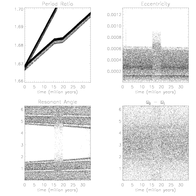
Figure 3: The evolution of two planets illustrated in Fig. 3 but with two additional outer planets added after the disk migration phase as indicated in the text. The upper right panel shows the evolution of the period ratio of the innermost two planets under orbital circularization. The uppermost curve is for $Q^{\prime}=1.5$ and the lower curve is for $Q^{\prime}=3.$ The evolution of the eccentricity of the second innermost planet is plotted in the upper left panel. The evolution of the resonant angle $3\lambda_{2}-2\lambda_{1}-\varpi_{1}$ is plotted in the lower left panel. The behaviour of the angle between the apsidal lines of the orbits of the second innermost and innermost planets is illustrated in the lower right panel.

4.7 Adding additional planets

Here the effect of adding additional planets to the simulation described above is investigated. To do this we take the calculation of section 4.6 at the point at which forces arising from the disk cease to act. Two additional planets of masses $5.36M_{\oplus}$ and $7.09M_{\oplus}$ are added in circular orbits with semi-major axes $0.07au$ and $0.22au$ respectively. These correspond to the two outermost planets in the GJ581 system. We remark that the eccentricities of these planets were determined to be consistent with zero by Vogt et al. (2010). As before we considered runs for which $Q^{\prime}=1.5$ and $Q^{\prime}=3.$ In this case the same value of $Q^{\prime}$ was adopted for each planet.

The results are plotted in Fig. 3. The evolution in this case is for the most part similar to that illustrated in Fig. 2 for two planets. In particular approximately the same time is taken for the period ratio for the innermost pair of planets to move from $5/3$ to $1.7.$ However, a significant difference is that the evolution of the period ratio slows down briefly between $1.5\times 10^{7}$ and $2.0\times 10^{7}yr.$ in the simulation with $Q^{\prime}=3.$ During this time the eccentricity of the second innermost planet is increased. Although the reasons for this are unclear, it is associated with an interaction between the second and third innermost planets. The innermost planet continues to move inwards but the angular momentum ends up being transferred to the third rather than the second innermost planet. There does not seem to be any clear resonance associated with this. However, we comment that in a many planet system like this, we could consider a tension between possible interacting pairs. The second and third planets would separate on account of tidal circularization if the innermost planet were absent. Similarly the innermost pair can couple as in section 4.6. In some circumstances, dependent on their masses, orbital parameters, and values of $Q^{\prime}$ etc., different interacting pairs may have varying levels of importance in the simulation. This requires a more detailed study than we have been able to perform at this preliminary stage that will be the subject of future work.

4.8 A system with a 3:1 commensurability

Finally we describe a situation in which a $3:1$ commensurability could be formed under convergent migration and then subsequently maintained. The parameters of this simulation were chosen to lead to a separation of pairs similar to the third and fourth innermost planets in the HD 10180 system for which there may have been a past proximity to a 3:1 commensurability.

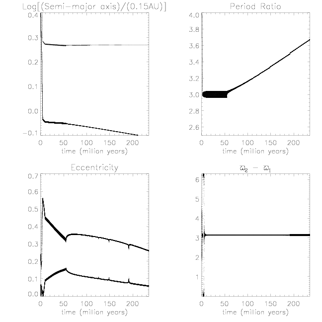
Figure 4: The evolution of two planets in a 3:1 commensurability is illustrated. The left uppermost panel shows the evolution of the semi-major axes of the two planets. The initial period of disk migration is short $<\sim 4.5\times 10^{6}yr.$ The subsequent evolution is driven by tidal circularization with $Q^{\prime}=100$ and the gravitational interaction between the planets. The upper left panel shows the evolution of the period ratio. This remains 3:1 for some time after disk migration has ceased before finally increasing as the planets separate. The lower left panel shows the evolution of the eccentricities of the two planets, the uppermost curve corresponding to the inner planet. The lower right panel shows the angle between the apsidal lines of the orbits of the outer and inner planets, which ultimately remains close to $\pi.$

In this case the central mass was taken to be $1M_{\oplus}.$ The inner planet mass was taken to be $11.73M_{\oplus}$ and the outer planet taken to be $25.07M_{\oplus}.$ Their initial semi-major axes were $0.387au$ and $1.2au$ respecively. The outer planet was started in circular orbit while the inner planer was started at apocentre with an eccentricity $e=0.24.$ The disk migration and circularization rates adopted were given by

$$t_{mig}=t_{c,i}=1.4\times 10^{8}\frac{M_{\oplus}}{m_{i}}yr.$$ (60)

These were applied only when the planets semi-major axes exceeded $0.29au.$ Note that this migration rate is very much lower than the previous cases so as to enable trapping in the $3:1$ resonance. The ecentricity damping rate is taken to be equal to the migration rate so that the eccentricities do not damp too quickly so enabling the 3:1 resonance to persist. Rates like these are not readily produced in calculations of disk planet interactions for which the planets are fully embedded. They may be possible if the planets are located within a wide cavity. However, this aspect remains to be investigated. Here we simply adopt these rates and explore their consequences. Because of the larger planetary masses and larger orbital eccentricities in this run, it was possible to consider larger values of $Q^{\prime}.$ We adopted $Q^{\prime}=100.$

The evolution of the two planets in this simulation is illustrated in Fig. 4. The planets undergo convergent migration and attain a 3:1 resonance. The eccentricity of the inner planet grows up to $\sim 0.56.$ The growth ceases after $\sim 4\times 10^{6}yr.$ when effects arising from the disk cease to act. After this time the planets evolve under tidal circularization. For about $50$ million years the commensurability is maintained while the eccentricty of the inner planet decreases and that of the outer one increases. In this process angular momentum is transferred to the inner planet. However, this form of evolution cannot be maintained and it reverts to the situation where the planets separate in semi-major axis as descibed in section 2.1 while the eccentricities decrease. The period ratio secularly increases while the angle between the apsidal lines of the orbits of the outer and inner planets remains close to $\pi.$

Interestingly at least five resonance passages were seen during this later evolutionary stage. As the period ratio increased, these corresponded to the 19:6, 16:5, 13:4, 10:3 and 7:2 resonances. They are manifested as local blips in the eccentricity evolution of both planets as shown in the lower left panel of Fig. 4. The resonance passages are of decreasing order with increasing time and so the consequent changes induced in the planetary eccentricities increase in magnitude. The fact high order resonances such as $19:6$ were manifest in this run is because of the relatively high eccentricities, in particular of $\sim 0.3$ for the inner planet.

5 Discussion

In this paper we have studied systems of close orbiting planets evolving under the influence of tidal circularization. We considered the situation where the system evolved under the influence of disk tides to form a commensurability. After the disk tides ceased to operate, either because of entry into an inner cavity, or because of loss of the disk, the operation of tidal circularization caused increasing departure from any close commensurability as time progressed.

In section2.1 we pointed out that a system of planets in near circular orbits is expected to separate on average as energy is dissipated while angular momentum is conserved. This is also expected in the very similar situation of an accretion disk evolving under a viscosity (see Lynden-Bell & Pringle 1974). In the simplest case of two planets, this inevitable increasing physical separation has to lead to the increasing departure from any initial commensurability.

In sections 2.2, 2.3 and 3, we developed a formalism that could be adapted study the evolution of two planets near to a first order commensurability under the influence of tidal circularization. This was then applied to a system with a tight commensurability in section 3.1. An expression for the departure from commensurability, indicating this to be $\propto t^{1/3},$ was given (see equation (42)). The discussion was then extended to the situation when the two planets were not necessarily in a close commensurability in section 3.2. The orbital evolution of the planet in that case, leading to a neighbouring commensurability, was then considered in section 3.3.

In order to confirm the analytic modeling, numerical simulations were under taken in section 4. We were able to set up systems of low mass planets in varying commensurabilities, depending on the strengths of the disk tides leading to orbital migration and circularization, with weaker tides in general leading to more widely separated commensurabilities. We focused on a two planet system which had the same parameters as the innermost two planets as the GJ581 system in section 4.5. This formed a 3:2 commensurability which then evolved under orbital circularization. This model system attained the period ratio of the actual system after $\sim 10^{8}yr.$ when $Q^{\prime}\sim 1.$ Simple extrapolation thus indicates that tidal evolution could have moved the system to the present period ratio of $1.7$ from a 3:2 commensurability if $Q^{\prime}\sim 100.$ Similarly the situation when the system initially attained a 5:3 commensurability was studied in section 4.6. In this case the evolution quickly adapted to evolve as for the case with the initial 3:2 commensurability when that had reached the same period ratio. However, a larger value $Q^{\prime}$ would suffice to cause the period ratio to move from 5:3 to the observed one within a given life time. The effect of adding the additional planets in the GJ581 system was considered in section 4.7. In that case over the long term the extra planets did not greatly affect the evolution. However, for a brief period the third planet moved outwards taking up the angular momentum of the innermost planet rather than the second, with the consequence that the period separation rate for the innermost pair was slowed. Thus a pair of planets may not always evolve independently of others in the system, a feature that requires further study.

Finally the evolution of a system that formed a 3:1 commensurability was considered in section 4.8. The model system adopted had similar parameters to the third and fourth innermost planets in the HD 10180 system. This case required slow disk migration and weak circularization with the result that the resonance involved high eccentricities. Because of these the commensurability could be maintained for a while under orbital circularization. However, eventually the system increasingly departed from it as in the other cases. Finally all of our results indicate that if $Q^{\prime}<\sim 100,$ commensurabilities would have been significantly affected by tidal effects related to orbital circularization. Thus the survival of close commensurabilities in observed systems may be indicative of the presence of large $Q^{\prime}$ values, a feature which in turn may be related to the internal structure of the planets involved.

- (1) Barnes, R., Jackson, B., Raymond, S. N., West, A. A., Greenberg, R.: The HD 40307 Planetary System: Super-Earths or Mini-Neptunes? ApJ, 695, 1006-1011 (2009)
- (2) Bonfils, X., Forveille, T., Delfosse, X., et al.: The HARPS search for southern extra-solar planets. VI. A Neptune-mass planet around the nearby M dwarf Gl 581. A&A, 443, L15-L18 (2005)
- (3) Brouwer, D., Clemence, G. M.: Methods of celestial mechanics, 416-421. Academic Press, New York (1961)
- (4) Brunini, A., Cionco, R. G.: The origin and nature of Neptune-like planets orbiting close to solar type stars. Icarus, 177, 264-268 (2005)
- (5) Goldreich, P., Soter, S.: Q in the Solar System. Icarus, 5, 375-389 (1966)
- (6) Lovis, C., S gransan, D. Mayor, M., et al.: The HARPS search for southern extra-solar planets. XXVII. Up to seven planets orbiting HD 10180: probing the architecture of low-mass planetary systems. A&A, In press (2010)
- (7) Lynden–Bell, D., Pringle, J. E.: The evolution of viscous discs and the origin of the nebular variables. MNRAS, 168, 603-637 (1974)
- (8) Mayor, M., Bonfils, X., Forveille, T., et al.: The HARPS search for southern extra-solar planets. XVIII. An Earth-mass planet in the GJ 581 planetary system. A&A, 507, 487-494 (2009)a
- (9) Mayor, M., Udry, S., Lovis, C., et al.: The HARPS search for southern extra-solar planets. XIII. A planetary system with 3 super-Earths (4.2, 6.9, and 9.2 ). A&A, 493, 639-644 (2009)b
- (10) Murray, C. D., Dermott, S. F.: Solar System Dynamics. 254-255, Cambridge University Press, Cambridge England (1999)
- (11) Papaloizou, J.C.B.: Disc-Planet Interactions: Migration and Resonances in Extrasolar Planetary Systems. Cel. Mech. and Dynam. Astron., 87, 53-83 (2003)
- (12) Papaloizou, J. C. B., Larwood, J. D.: On the orbital evolution and growth of protoplanets embedded in a gaseous disc. MNRAS, 315, 823- 833 (2000)
- (13) Papaloizou, J.C.B., Szuszkiewicz, E.: On the migration-induced resonances in a system of two planets with masses in the Earth mass range. MNRAS, 363, 153-176 (2005)
- (14) Papaloizou, J.C.B., Szuszkiewicz, E.: Conditions for the occurrence of mean-motion resonances in a low mass planetary system. EAS Publications Series, 42, 333-343 (2010)
- (15) Papaloizou, J.C.B., Terquem, C.: Dynamical relaxation and massive extrasolar planets. MNRAS, 325, 221-230 (2001)
- (16) Papaloizou, J.C.B., Terquem, C.: On the dynamics of multiple systems of hot super-Earths and Neptunes: tidal circularization, resonance and the HD 40307 system. MNRAS, 405, 573-592 (2010)
- (17) Paardekooper, S.–J, Mellema, G.: Halting type I planet migration in non-isothermal disks. A&A, 459, L17-L 20 (2006)
- (18) Paardekooper, S.–J, Papaloizou, J. C. B.: On disc protoplanet interactions in a non-barotropic disc with thermal diffusion. A&A, 485, 877- 895 (2008)
- (19) Paardekooper, S.–J, Papaloizou, J. C. B.: On corotation torques, horseshoe drag and the possibility of sustained stalled or outward protoplanetary migration. MNRAS, 394, 2283-2296 (2009)
- (20) Raymond, S. N., Barnes, R., Mandell, A. M.: Observable consequences of planet formation models in systems with close-in terrestrial planets. MNRAS, 384, 663-674 (2008)
- (21) Schlaufman, K. C., Lin, D. N. C., Ida, S.: The Signature of the Ice Line and Modest Type I Migration in the Observed Exoplanet Mass-Semimajor Axis Distribution. Apj, 691, 1322-1327 (2009)
- (22) Sinclair, A. T.; The orbital resonance amongst the Galilean satellites of Jupiter. MNRAS, 171, 59-72 (1975)
- (23) Tanaka, H., Takeuchi, T., Ward, W. R.: Three-Dimensional Interaction between a Planet and an Isothermal Gaseous Disk. I. Corotation and Lindblad Torques and Planet Migration. ApJ, 565, 1257-1274 (2002)
- (24) Terquem, C., Papaloizou, J. C. B.: Migration and the Formation of Systems of Hot Super-Earths and Neptunes. ApJ, 654, 1110-1120 (2007)
- (25) Udry, S., Bonfils, X., Delfosse, X., et al.: The HARPS search for southern extra-solar planets. XI. Super-Earths (5 and 8 ) in a 3-planet system. A&A, 469, L43-L47 (2007)
- (26) Vogt, S. S., Butler, R. P., Rivera, E. J. et al.: The Lick-Carnegie Exoplanet Survey: A 3.1 Planet in the Habitable Zone of the Nearby M3V Star Gliese 581. ApJ, 723, 954-965 (2010)
- (27) Ward, W. R.: Protoplanet Migration by Nebula Tides. Icarus, 126, 261-281 (1997)