Exact Kohn-Sham eigenstates versus quasi-particles in simple models of strongly correlated electrons

Abstract

We present analytic expressions for the exact density functional and Kohn-Sham Hamiltonian of simple tight-binding models of correlated electrons. These are the single- and double-site versions of the Anderson, Hubbard and spinless fermion models. The exact exchange and correlation potentials keep the full non-local dependence on electron occupations. The analytic expressions allow to compare the Kohn-Sham eigenstates of exact density functional theory with the many-body quasi-particle states of these correlated-electron systems. The exact Kohn-Sham spectrum describes correctly many of the non-trivial features of the many-body quasi-particle spectrum, as for example the precursors of the Kondo peak. However, we find that some pieces of the quasi-particle spectrum are missing because the many-body phase-space for electron and hole excitations is richer.

I Introduction

Density Functional Theory Hohenberg64 ; Kohn65 allows to tackle complex quantum systems comprising $N$ interacting electrons. Its essence consists on the replacement of the extremely convoluted many-particle electronic interactions with an effective one-body potential, also known as the exchange and correlation potential $V^{XC}$, whereby the $N$-particle Hamiltonian is substituted by a fictitious one-particle Kohn-Sham Hamiltonian $H^{KS}$. The exact $V^{XC}$ is however not known and it is a widespread belief that it is not possible to find an analytic exact expression for it. The popularity of Density Functional Theory (DFT) has arisen from the fact that semi-empirical fittings of $V^{XC}$ to the exchange and correlation potential of the Jellium model in the Local Density Approximation (LDA) and improvements over itPerdew81 ; Perdew96 ; Becke93 perform remarkably well for a large majority of materials, molecules and nanostructures. The qualitative features of the structural and functional properties of many systems are usually well reproduced, and in a number of cases, quantitative agreement can also be reached. However, these practical implementations of DFT are not perfect. They fail to predict a number of relevant properties, specially for strongly correlated electronic systems. Yang and coworkers have discussed some explicit conditions that exact energy functionals must obeyCohen08b ; Mori09 .

DFT has also been proposed for tight-binding models of strongly correlated electronsSchonhammer95 . The availability of exact semi-analytical or numerical results for the ground state energy as a function of the electron concentration in the Hubbard and the spinless fermion modelsLieb68 ; Yang66 has allowed to establish a Bethe ansatz LDA theory for themSchonhammer95 ; Lima03 ; Schenk08 . An extension of the theory to describe time-dependent external potentials has enabled the description of non-equilibrium electron transport phenomenaVerdozzi08 ; Kurth10 ; Burke11a . However, Bethe ansatz LDA theory also has limitations. First, since the Bethe Ansatz solution expresses the ground-state energy in terms of the electron concentration, only a local density approximation could be formulated. Second, the analytic formula for ground state energy is exact only at half-filling, while away from it semi-analytical or numerical fittings to the solution of the Bethe Ansatz equations must be performed. Finally, inhomogeneous systems where strong correlations take place in localized region of them are better described by Anderson models. However, the Anderson model is Bethe Ansatz-solvable only if the band of uncorrelated electrons is linearizedTsvelick83 , leaving the system energy unbounded from below. Therefore, the ground state energy can not be obtained by a minimization procedure, which renders the Bethe ansatz LDA approach useless for the Anderson model.

The quasi-particle (QP) excitation spectrum of a system determines its response to external perturbations according to Landau’s Fermi liquid theory. Furthermore, this spectrum is directly accessible via spectroscopic techniques of different sorts. It would therefore be quite useful if the Kohn-Sham (KS) eigenstates provided at least a qualitative description of it, as one would expect to happen at least for systems where electronic correlations are weak. This is indeed confirmed by a vast amount of calculations and comparisons between KS eigenvalues and experimental or numerical data of weakly correlated materials. However, quantitative agreement is sometimes not so good. Furthermore the KS spectrum is frequently qualitatively wrong in strongly-correlated materials. Notice now that even if the exact $V^{XC}$ of a specific system is known, a possible correspondence between the exact KS and the exact many-body QP spectra is not supported at all by the basic theorems of DFT. An exception is the Highest Occupied Molecular Orbital (HOMO) which by Janak’s theorem is given by the chemical potential of the system, which is a ground-state propertyJanak78 ; Perdew83 ; Sham83 . In other words, DFT predicts the correct position of the HOMO level of a system, provided that the exact $V^{XC}$, or a very good approximation to it, is known. Failures to predict the correct position of the HOMO must therefore be attributed to a poor approximation to the exact $V^{XC}$. Failures to reproduce the rest of the spectrum could however be due either to limitations of DFT proper, or to a poorly approximated functional. Indeed, while an exact functional may not provide a good description of the full QP spectrum, it is clear that if in addition, the quality of the approximate functional is poor, the proposed spectrum of KS eigenvalues will bear a small resemblance to the true QP spectrum. Since no exact functional for a strongly correlated system has ever been developed, the above two sources of disagreement have never been fully disentangled. The main goal of this article is to separate them. We will find the exact KS eigenvalues of several simple models of strongly correlated electrons and compare them with the exact many-body QP spectrum. This will allow us to understand the size of the self-energy corrections to the exchange-correlation potential.

One of the main sources of disagreement between approximate DFT KS eigenvalues and exact QP originates in the mean-field-like treatment of electronic correlations which lie at the heart of LDA. Indeed, electrons behave as quantum point particles. However, mean-field theories replace quantum probabilities by classical clouds of charge. As a result, every electron may interact with its own charge cloud, giving rise to spurious direct and exchange self-interaction effects. Additionally, each electron interacts with the clouds of other electrons having opposite spin, leading to what is sometimes called the static correlation errorCohen08b . For systems containing more than one atom, these mean field clouds are spread throughout the whole entity in contrast to electrons which are always point particles and therefore fully localized. This spread gives rise to further spurious effects termed delocalization errors, which lead to incorrect dissociation energies and QP excitation energies for moleculesCohen08b . A prototypical example of the delocalization error is an $H_{2}^{+}$ molecule in the dissocation limit where the two ions are held widely apart. The single electron in the molecule has equal probability of residing in any of the two atoms, but a measuring proccess will find it fully localized in only one of them. Mean field theories in contrast place half an electron in each ion. The excitation energy of an added quasi-electron will therefore be different in the two casesRomaniello09 ; Explanation .

Improving the description of the QP spectrum therefore implies improving the description of electronic correlations. The Hartree-Fock approximation as well as the self-interactions correction schemePerdew81 ; Rieger95 ; Filippetti03 ; Toher09 get rid of the self-interaction effect, but not of other mean-field drawbacks. To go beyond these schemes, the Dyson-Sham-Schlüter equation must be used

$$G=G_{approx}^{KS}+G_{approx}^{KS}\,(\Sigma^{XC}-V_{approx}^{XC})\,G$$ (1)

where $G_{approx}^{KS}$ is the Green’s function obtained from the approximate KS Hamiltonian. Notice that $G_{approx}^{KS}$ carries already a mean-field description of the electron interaction. A perturbative expansion for the self-energy $\Sigma^{XC}$ must then be set up to improve the description of correlations and in particular to amend the destruction of quantum effects brought about by the mean-field approximation. The GW approximationHedin65 has been quite successful in the description of electronic and optical properties directly linked to the QP spectrumAulbur99 ; Onida02 , but does not correct the problems mentioned above. Some recent work by Romaniello and coworkers show how the careful inclusion of vertex corrections allows to get rid not only of the self-interaction effects but also of part of the delocalization effectsOnida02 ; Bruneval05 ; Romaniello09 . However, delocalization debris remains since molecular dissociation is still not well handled. In addition, Millis and coworkersWang08 ; Thygesen08 have studied the performance of the GW approximation for the Anderson model, and shown how this approximation can describe Coulomb blockade effects, but fails to describe the emergence of Kondo PhysicsHewsonBook ; Ferrer87 . Dynamical Mean Field Theory, implemented together with an accurate impurity-solver, includes many of the most relevant short-range correlation effectsSun04 ; Kotliar06 ; Jacob10 ; Korytar11 .

We have devised a procedure that has allowed us to find analytic expressions for the exact energy density functional of the single- and double-site Anderson, Hubbard and spinless fermion models, from which we have been able to write down the corresponding exact Hamiltonians $H^{KS}$. Since the QP spectrum of these models is available analytically from conventional many-body techniques, we have been able to perform explicit and detailed comparisons of the full spectra of exact KS eigenvalues and of exact many-body QP. We have found that the KS eigenvalue corresponding to the HOMO level agrees with the corresponding QP state. This implies that the exact $H^{KS}$ correctly predicts that the lowest energy for electron addition of an $N$-electron system is equal to the highest energy for electron removal of the corresponding $N+1$ systemRomaniello09 . We have also found that the exact $H^{KS}$ of the Anderson model describes correctly the emergence of the Kondo resonance and of other quasi-particles. However, we find that there exact density functional theory misses pieces of the exact many-body QP spectrum. A way to improve the description of the spectrum would be to use again the Dyson-Sham-Schlüter equation

$$G=G_{exact}^{KS}+G_{exact}^{KS}\,(\Sigma^{XC}-V_{exact}^{XC})\,G$$ (2)

where $G_{exact}^{KS}$ is the Green’s function associated to the exact KS Hamiltonian. We expect that this self-energy and its perturbative expansion should be much simpler than the self-energy defined in Eq.(1) above, because now the unperturbed Green’s function retains the full quantum nature of electrons. Our piece of work is complementary to efforts by other groups to provide exact functionals for simplified systems. We mention here recent work by Burke and collaborators, who have found numerically exact density functionals for some one-dimensional models by combining DFT with Density Matrix Renormalization Group techniquesBurke11b .

The layout of this article is as follows. Section II describes the methodology employed to find out exact functionals for systems with a small number of electrons. This methodology is applied in sections III and IV to describe the single-site Hubbard model, and the double-site Anderson model, respectively. The conclusions are laid down in section V. The solution of the double-site Hubbard model is placed in appendix A. The solution of the double-site spinless fermion model can be found in appendix C.

II Methodology

We begin with a description of our method, which is based on the formulation of DFT on a latticeSchonhammer95 . We have found that the conventional ensemble-based method to describe non-integer occupationsLevy79 ; Perdew83 fails in the formulation of the exact density functional of the single-site model described below. We have therefore devised an alternative method which is specifically adapted for the description of quantum systems with a small but not necessarily integer number of electrons $N$.

We consider a physical system whose time-evolution is dictated by a tight-binding Hamiltonian. As an example, we write explicitly the Hamiltonian of the Anderson model,

$$\hat{H}= \sum_{i,\sigma}\,\epsilon_{c}\,\hat{n}_{c,i,\sigma}\,+\,\sum_{\sigma}\,\epsilon_{d}\,\hat{n}_{d,\sigma}\,-\,\sum_{i,\sigma}\,t_{0}\,(\hat{c}_{i,\sigma}^{\dagger}\,\hat{c}_{i+1,\sigma}+h.c.)\,$$ (3)

$$-\,t\,\sum_{\sigma}\,(\hat{c}_{1,\sigma}^{\dagger}\,\hat{d}_{\sigma}+h.c.)\,+\,U\,\hat{n}_{d,\uparrow}\,\hat{n}_{d,\downarrow}$$

where a set of $N$ electrons hop back and forth along a chain of $i=1,..,{\cal M}$ atoms, labeled by the index $c$, and to another atom, denoted by the index $d$, where electron correlations take place via a Coulomb term $U$. The $\sigma-$index denotes the up and down components of the electron spin.

We use the Fock space of states of the system $\{|\,\phi>\}$ to set up our variational scheme. Site occupations, electron numbers and the expectation value of the Hamiltonian are given by

$$n_{\alpha,\sigma}(\phi)\, = \,\frac{<\phi\,|\,\hat{n}_{\alpha,\sigma}\,|\,\phi>}{<\phi\,|\,\phi>}$$

$$N_{\sigma} = \sum_{i}n_{c,i,\sigma}+n_{d,\sigma}$$

$$E(\phi)\, = \,\frac{<\phi\,|\,\hat{H}\,|\,\phi>}{<\phi\,|\,\phi>}$$ (4)

We wish to define an energy density functional $Q[n_{c,i,\sigma},n_{d,\sigma^{\prime}},U]$ whose minimization gives the exact ground state energy $E^{0}$ and occupations $n_{i,\sigma}^{0}$ for a target set of electron numbers $(N_{\uparrow}^{0},N_{\downarrow}^{0})$. To define $Q$, we note that every given set of occupations $\{n_{c,i,\sigma},n_{d,\sigma^{\prime}}\}$ can be reproduced by several states $|\,\phi>$. In other words, if we classify these states in boxes labeled by each occupation set, then each box contains several $|\,\phi>$, and each of these has a different energy $E(\phi)$. However, if we choose in each box the state $|\,\phi^{m}>$ with minimum energy $E^{m}=E(\phi^{m})$, we achieve a one-to-one correspondence between occupation sets and energies for every box, which allows to define the energy density functional $Q[n_{c,i,\sigma},n_{d,\sigma^{\prime}},U]=E^{m}$Provided . Since there exist in general several sets of occupation numbers $\{n_{c,i,\sigma},n_{d,\sigma^{\prime}}\}$ giving the same target electron numbers $N_{\sigma}=N_{\sigma}^{0}$, the ground state energy $E^{0}$ is obtained by minimizing $Q$ over all those sets. This procedure then defines the ground state occupations $\{n_{c,i,\sigma}^{0},n_{d,\sigma^{\prime}}^{0}\}$.

We define now the non-interacting kinetic energy functional $T[n_{c,i,\sigma},n_{d,\sigma^{\prime}}]=Q[n_{c,i,\sigma},n_{d,\sigma^{\prime}},U=0]$, and the Exchange-correlation functional $E^{XC}=Q-T$, from which the exact Exchange-correlation potential $V^{XC}$ is obtained by taking partial derivatives

$$V_{c,i,\sigma}^{XC}[n_{c,i^{\prime},\sigma^{\prime}},n_{d,\sigma^{\prime\prime}}]\, = \,\frac{\partial E^{XC}}{\partial n_{c,i,\sigma}}\,\,\,\,\,\,\,\,\,i=1,{\cal M}$$

$$V_{d,\sigma}^{XC}[n_{c,i^{\prime},\sigma^{\prime}},n_{d,\sigma^{\prime\prime}}]\, = \,\frac{\partial E^{XC}}{\partial n_{d,\sigma}}$$ (5)

We do not use a Hartree term in the definition of $E^{XC}$ because we have found no traces of such a term in the analytic equations for the exact functionals. Therefore we have found it useless for the purposes of the present discussion. We define the exact KS Hamiltonian as follows:

$$H^{KS}= \sum_{i,\sigma}(\epsilon_{c}\,+V_{c,i,\sigma}^{XC})\,\hat{n}_{c,i,\sigma}+\sum_{\sigma}(\epsilon_{d}+V_{d,\sigma}^{XC})\,\hat{n}_{d,\sigma}$$ (6)

$$-t\,\sum_{i,\sigma}\,(\hat{c}_{i,\sigma}^{\dagger}\,\hat{d}_{\sigma}\,+\,\hat{d}_{\sigma}^{\dagger}\,\hat{c}_{i,\sigma}\,)-E_{dc}$$

where $E_{dc}$ is a double-counting term. Notice that the above procedure allows to define functionals and KS Hamiltonians for systems with a fractional electron number. However, the many-body Hamiltonian in Eq. (3) commutes with the electron number operator $N_{\sigma}$. Therefore the many-body Hamiltonian eigenstates must describe an integer number of electrons, unless some degeneracy occurs. We will see later on that the functional $Q$ has a polygonal shape, so that the Exchange-correlation potentials jump by constants at integer $N_{\sigma}$ values, which lead to ambiguous definitions of the KS eigenvalues at integer $N_{\sigma}$. However, the total energies of the ground- and excited-states of the KS Hamiltonian $E^{\alpha}$ ($\alpha=0,1,...$) are continuous because the the jumps in the summations over KS eigenvalues are counterbalanced by similar jumps in the double-counting terms. The ground state energy $E^{0}$ of the exact KS Hamiltonian and many-body Hamiltonians agree with each other by construction, but this is not so for the total energies of the excited states of both Hamiltonians, which are needed to construct the Green’s functions.

The QP spectrum of the many-body Hamiltonian can be compared with the KS and mean-field spectra by looking at the poles and residues of the Green’s functions $G(\omega)$, $G^{KS}(\omega)$ and $G^{MF}(\omega)$. We define on this matter the many-body HOMO level as the QP peak which is partially filled. The exact $G$ and $G^{KS}$ need not agree, except for the pole describing the HOMO level. We will use the Lehmann representationMahanBook to compute $G$ for integer $N$-values. In addition, the equations-of-motion methodLunquist yields a closed set of equations for $G$ for the single-site model. This method nicely enables to extrapolate the $G$-poles to non-integer electron numbers, and agrees with the results obtained using the Lehmann representation for integer $N$. The mean field spectrum can be obtained from the eigenvalues of the one-body mean-field Hamiltonian, or using the equations-of-motion method for $G^{MF}$. The KS spectrum could also be obtained from the eigenvalues of the one-body KS Hamiltonian. However, these KS eigenvalues are discontinuous at $N$ integer so ambiguities in the ascription of eigenvalues to QPs arise for integer $N$. It is therefore essential to use the Lehmann representation as a guide.

We close this section by describing an alternative procedure which also allows us to find exact results. If the exact ground state energy $E^{0}$ and occupations $n^{0}_{i,\sigma}$ are found then the Schrödinger equation for the Kohn-Sham hamiltonian can be inverted to find the exact exchange and correlation potential corresponding to the ground state occupations $v^{XC}_{i,\sigma}=V^{XC}_{i,\sigma}[n_{j,\sigma^{\prime}}^{0}]$. We note however that $v^{XC}_{i,\sigma}$ is not a functional, but rather corresponds to the Exchange-correlation potential functional evaluated at the ground state occupations. This procedure is simpler than the methodology described in this section, but does not allow us to find functionals. Similar methods have been employed by Baerend and coworkersGritsenko96 , as well as by Helbig and coworkersHelbig09 to find exact analytical or numerical expressions for the Exchange-correlation potential of diatomic molecules in the dissociation limit.

III Single-site Anderson-Hubbard model

The above methodology can be easily applied to the single-site Anderson-Hubbard model (${\cal M}=0$), where only two occupations $\{n_{d,\uparrow},n_{d,\downarrow}\}$ are defined. The states in the Fock space of the single-site model can be expressed using the number basis $|n_{d,\uparrow},n_{d,\downarrow}>$ as

$$|\,\phi>\,=\,a_{0}\,|\,0,0>\,+\,a_{\uparrow}\,|\,1,0>\,+\,a_{\downarrow}\,|\,0,1>\,+\,a_{2}\,|\,1,1>$$ (7)

The expectation value of the occupation numbers and the energy can then be expressed as

$$n_{d,\sigma}(\phi) = \frac{|a_{\sigma}|^{2}+|a_{2}|^{2}}{D}$$

$$E(\phi) = \sum_{\sigma}\,\epsilon_{d}\,n_{d,\sigma}+\,U\,\frac{|a_{2}|^{2}}{D}$$ (8)

where $D={|a_{0}|^{2}+|a_{\uparrow}|^{2}+|a_{\downarrow}|^{2}+|a_{2}|^{2}}$. The simplest way to find $Q[n_{d,\uparrow},n_{d,\downarrow}]$ is as follows. Solve first for some of the coefficients $a_{i}$ using the occupations for the occupation numbers $n_{d,\sigma}$. Those coefficients are then eliminated by inserting them back into the equation for $E(\phi)$. The resulting expression is then minimized in terms of the remaining coefficients. One must be careful though to choose coefficients which are strictly non-zero in a given domain of $N$. In the present case, it is best to solve for $a_{\sigma}$ since these are finite for all $N=n_{d,\uparrow}+n_{d,\downarrow}$ different from $0,2$:

$$(1-N)\,(|a_{\uparrow}|^{2}+|a_{\downarrow}|^{2})=N\,|a_{0}|^{2}+(2-N)\,|a_{2}|^{2}$$ (9)

The resulting equation for

$$E(\phi)=\sum_{\sigma}\,\epsilon_{d}\,n_{d,\sigma}+\,U\,(N-1)\,\frac{|a_{2}|^{2}}{|a_{2}|^{2}-|a_{0}|^{2}}$$ (10)

is minimized as

$$\begin{array}[]{ccccl}0<N<1&\rightarrow&|a_{2}|^{2}=0\rightarrow&Q=&\epsilon_{d}\,N\\ 1<N<2&\rightarrow&|a_{0}|^{2}=0\rightarrow&Q=&\epsilon_{d}\,N+U\,(N-1)\end{array}$$ (11)

The above expressions for the exact functional $Q$ can be summarized as

$$Q[n_{d,\uparrow},n_{d,\downarrow}]=\epsilon_{d}\,N\,+\,U\,(N-1)\,\theta(N-1)$$ (12)

where $\theta$ is the Heaviside step function. This expression gives the correct ground state energy for a system with a target number $N_{\uparrow}^{0},N_{\downarrow}^{0}$ of electrons

$$E^{0}=\epsilon_{d}\,N^{0}+U\,(N^{0}-1)\,\theta(N^{0}-1).$$ (13)

Note that this ground state energy is spin-degenerate. Subtracting from $Q$ the non-interacting kinetic energy functional $T[n_{d,\uparrow},n_{d,\downarrow}]=\epsilon_{d}\,N$, and taking a functional derivative, we find the exact Exchange-correlation potential $V_{d,\sigma}^{XC}=U\,\theta(N-1)$. The resulting KS Hamiltonian

$$H^{KS}=\sum_{\sigma}(\epsilon_{d}+U\,\theta(N-1))\,\hat{n}_{d,\sigma}-U\,\theta(N-1)$$ (14)

provides the correct $E^{0}$ thanks to the double counting term $U\,\theta(N^{0}-1)$. Notice that the KS eigenvalue jumps by $U$ exactly at $N=1$, and is therefore ill-defined at that integer $N$-valuePerdew81 ; Perdew82 ; Perdew83 ; Janak78 . The density functional $Q$ has the correct trapezoidal shapePerdew82 ; Cohen08b as a function of $N_{\sigma}$, from which the right expression for the chemical potential of the system can be obtained. Furthermore, $Q$ shows flat-plane behavior when plotted as a function of the occupation numbers, as displayed in Fig. 1. We note that Yang and coworkers established some exact conditions on the shape of the exact energy functional, from which they deduced such a flat-plane behaviorMori09 . These conditions enabled them to draw an educated plot of the energy functional of the hydrogen atom, which is very similar to our Fig. 1.

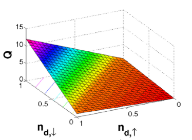
Figure 1: (Color online) Three-dimensional plot of the exact energy functional $Q$ of the single-site Anderson-Hubbard model as a function of $(n_{d,\uparrow},n_{d,\downarrow})$, for a value of $\epsilon_{d}=1$ and of $U=10$ (in arbitrary units).

We write down now the mean-field Hamiltonian of this model

$$H^{MF}=\sum_{\sigma}(\epsilon_{d}+U\,n_{d,-\sigma})\,\hat{n}_{d,\sigma}-U\,n_{d,\uparrow}\,n_{d,\downarrow}$$ (15)

where we have subtracted the conventional mean-field double-counting term. The mean-field Hamiltonian gives the following estimate for the energy of the system

$$E^{MF} = \epsilon_{d}\,N+U\,n_{d,\uparrow}\,n_{d,\downarrow}=\epsilon_{d}\,N+U\,\frac{N^{2}-M^{2}}{4}$$

$$M = n_{d,\uparrow}-n_{d,\downarrow}$$ (16)

where the spin-degeneracy of the exact solution is lost. Note that in the Hubbard and Anderson models every electron interacts only with electrons of opposite spin. As a consequence, the mean-field theory does not suffer from direct or exchange self-interaction effects. However, because of the mean-field replacement of electron probabilities by charge clouds, an electron of spin $\sigma$ interacts with a fraction $n_{d,-\sigma}$ of electrons of opposite spin, instead of with a full electron of opposite spin with probability $n_{d,-\sigma}$. As a consequence, in the paramagnetic solution $M=0$, every electron interacts artificially with a fraction $N/2$ of electrons of opposite spin. However, the mean-field ground state energy is minimized by the fully spin polarized solutions $M=N$, in which case the spurious interaction between opposite-spin charge clouds is avoided by a wrong mechanism and, as a consequence, $E^{MF}=E^{0}$. In contrast, the interacting piece of the exact KS Hamiltonian $U\,\theta(N-1)$ is only activated if a full electron exists already in the system, and therefore retains the full quantum behavior.

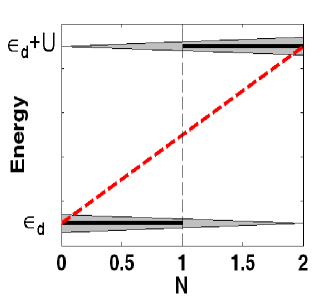
Figure 2: (Color online) Quasiparticle spectrum of the single-site Anderson-Hubbard model for $M=0$. The shaded gray area shows the position of the many-body poles, where the area is proportional to the weight of the peak. The black solid line represents the location of the exact Kohn-Sham eigenstate. The poles of the paramagnetic mean-field solution are shown with a dashed red line. Energy units are arbitrary.

The exact many-body and mean-field QP spectrum are obtained from the poles and weights of the retarded Green’s function

$$G_{d,\sigma}(\omega) = \frac{1-n_{d,-\sigma}}{\omega-\epsilon_{d}+i\delta}+\frac{n_{d,-\sigma}}{\omega-(\epsilon_{d}+U)+i\delta}$$

$$G_{d,\sigma}^{MF}(\omega) = \frac{1}{\omega-(\epsilon_{d}+U\,n_{d,-\sigma})+i\delta}$$ (17)

The above equations can easily be obtained using the equations-of-motion method and allow to extrapolate the QP spectrum to non-integer values of $n_{d,\sigma}$ which, coupled to the spin degeneracy of the total energy enable the exploration of different spin states.

We analyze first the paramagnetic state where $M=0$ and $n_{d,\sigma}=N/2$. The exact KS Green’s function is found by combining the equations-of-motion method with the Lehmann representation for $N=0,1,2$. The following formula summarizes the results

$$G_{d,\sigma}^{KS}(\omega) = \frac{\theta(1-N)}{\omega-\epsilon_{d}+i\delta}+\frac{\theta(N-1)}{\omega-(\epsilon_{d}+U)+i\delta}$$ (18)

and extrapolates them to non-integer-$N$-values. The many-body, exact DFT and mean field Green’s function are shown in Fig. 2 as a function of $N$. The many-body Green’s function has two poles, which can be viewed as the ancestors of the lower and upper Hubbard bands of the Hubbard and Anderson modelsHewsonBook . The position of these two poles depends neither on the occupation nor on the spin of the system. They are separated exactly by an energy $U$ and their weight shifts smoothly from one peak to the other as $N$ increases. Because exact DFT is a single-particle theory, its Green’s function yields a single peak per KS eigenvalues, whose weight equals one. A remarkable exception happens at $N=1$, where the KS eigenvalue show an abrupt change from $\epsilon_{d}$ to $\epsilon_{d}+U$. Notice that both eigenvalues contribute at $N=1$ with equal weight. The $N\rightarrow 1^{-}$ ($N\rightarrow 1^{+}$) KS eigenvalue exactly agrees with the many-body lower (upper) Hubbard band precursor. This non-trivial result allows to draw an important conclusion: even if KS eigenvalues show a jump at integer electron number values, the eigenvalues at both sides of the given $N$ contribute to the QP spectrum. To summarize, the positions and weights of the exact KS and many-body peaks coincide for integer numbers $N$, showing how exact DFT keeps the quantum nature of the electrons in spite of being a one-body theory. The abrupt shift at $N=1$ can be viewed as the way that exact DFT uses to retain that quantum nature: if there is less than one electron at the site, then there is no Coulomb interaction because the electrons does not interact with itself. If there is more than one electron, then the Coulomb interaction between point particles of opposite spin is activated, rising the energy by $U$. Notice that many-body and exact DFT agree on the value of HOMO level, which is also equal to the chemical potential $\mu$, defined as the derivative of the total energy with respect to the particle numberPerdew83 ; Sham83 .

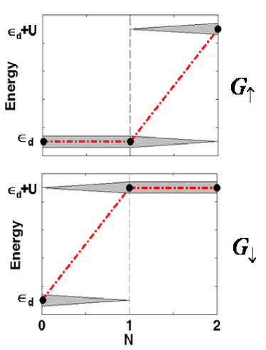
Figure 3: (Color online) Quasi-particle spectrum of the single-site Anderson-Hubbard model for a maximally spin-up polarized case. (a) and (b) show the poles of the spin-up and spin-down Green’s functions, respectively. The shaded gray area represents the many-body quasi-particle, where the width is proportional to the peak weight. The black thick dot represents the location of the exact Kohn-Sham eigenstates. The poles of the spin-polarized mean-field solution are shown with a dashed red line. Energy units are arbitrary.

We must remember however that in this quantum system only states with integer electron numbers $N_{\sigma}=0,1$ are meaningful. Therefore for $N=1$, the system must contain a full electron with either spin up or down. We therefore turn now to analyze a maximally spin-up polarized. The up- and down-spin Green’s functions are different now, as is apparent from the Lehmann representation at $N=1$, where we take $|1,0>$ as the ground state,

$$G_{d,\uparrow} = \frac{|<0,0|\,\hat{c}_{d,\uparrow}\,|1,0>|^{2}}{\omega+E_{1}-E_{0}+i\,\delta}$$

$$G_{d,\downarrow} = \frac{|<1,1|\,\hat{c}_{d,\downarrow}^{\dagger}\,|1,0>|^{2}}{\omega+E_{1}-E_{2}+i\,\delta}$$ (19)

where $E_{N}$ denote the total ground state energy for $N=0,1,2$. We determine now the many-body and mean field QP spectra for fractional occupation numbers using Eqs. (16). To determine $G^{KS}$ correctly for integer $N$ we use the Lehmann representation. The following formula extrapolates $G^{KS}$ to non-integer $N$-values

$$G_{d,\uparrow}^{KS}(\omega) = \frac{\theta(1-N+\delta)}{\omega-\epsilon_{d}+i\delta}$$

$$G_{d,\downarrow}^{KS}(\omega) = \frac{\theta(N-1+\delta)}{\omega-(\epsilon_{d}+U)+i\delta}$$ (20)

The different spectra are shown in Fig. 3. As before, the exact KS eigenvalues agree with the many-body QP for integer $N$. The mean-field states have a closer resemblance to the many-body QP, although clear differences still exist, whose origin is traced back to the static correlation error. As a closing remark, we note that the GW approximation cures these mean-field artifacts for the present case as shown by Romaniello and coworkersRomaniello09 .

IV double-site Anderson model

The model in the previous section has allowed to show how the exact density functional retains the quantum nature of electrons in a single atom and therefore avoids the static correlation error brought about by mean field theory. We wish to address in this section how the exact functional avoids also the delocalization error in a strongly-correlated model containing two sites. We show that the exact KS Hamiltonian provides a correct description of the atomic limit of the correlated model. The discussion is centered in the Anderson model, but our conclusions can be also applied to the double-site Hubbard model, which is solved in Appendix A. Notice that the many-body QP spectrum of the full Anderson model is much more complex than that of the single-site model discussed above and, in addition to the lower and upper Hubbard bands it develops a Kondo resonance in the Kondo regime. We therefore wish to explore now whether exact DFT could describe this more convoluted QP spectra. Finally, notice that the obtained energy functional $Q$ is spin-degenerate, in contrast to the full Anderson and Hubbard models, where this degeneracy is absent. It is therefore interesting to check whether exact DFT lifts the spin-degeneracy for more realistic models.

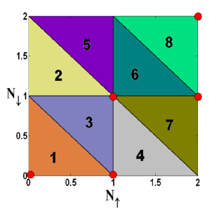
Figure 4: (Color online) The eight pieces in the $(N_{\uparrow},N_{\downarrow})$-plane which must be used to perform the constrained minimization procedure leading to the exact $Q$-functional of the double-site Anderson and Hubbard models. The thick dots indicate the positions where $G$ and $G^{KS}$ are evaluated.

We describe here the exact DFT solution of the double-site Anderson, which corresponds to taking ${\cal M}=1$ in Eq. (1), and can also be solved analytically. The number basis $\{|n_{c,\sigma}>,|n_{d,\sigma}>\}$ of the Fock space is spanned by sixteen states, which renders the minimization task of finding $Q[n_{c,\sigma},n_{d,\sigma}]$ asymptotically harder. We have found that the electron number plane $(N_{\uparrow},N_{\downarrow})$ is split into eight pieces as shown in Fig. 4, such that in each piece only a subset of the wave-function coefficients is different from zero. As a consequence, the minimization task has to be performed separately for each of those pieces. The $Q$-functional has again a polygonal shape. After lengthy algebra, the following expressions for the $Q$-functional in the symmetric case $\epsilon_{d}+U/2=\epsilon_{c}$ can be written:

$$\begin{array}[]{lll}F_{1}&=&-\left[\,\sqrt{n_{c,\uparrow}\,n_{d,\uparrow}}+\sqrt{n_{c,\downarrow}\,n_{d,\downarrow}}\,\right]\\ \\ F_{2}&=&-\left[\,\sqrt{(1-n_{c})\,(1-n_{d})}+2\,x\,\left(\sqrt{n_{c,\uparrow}-x^{2}}+\sqrt{n_{d,\uparrow}-x^{2}}\,\right)\,\right]+U\,x^{2},\,\,\,x=\frac{1}{2}\,\sqrt{N_{\uparrow}\,\left(1-\frac{U}{\sqrt{U^{2}+16\,t^{2}}}\right)}\\ \\ F_{3}&=&-\frac{1}{2}\,\left[\,\sqrt{(1+m_{c}-n_{d})\,(1+m_{d}-n_{c})}+\sqrt{(1-m_{c}-n_{d})\,(1-m_{d}-n_{c})}\right]+\frac{N-1}{4}\,\left(U-\sqrt{U^{2}+64\,t^{2}}\,\right)\\ \\ F_{4}&=&-\left[\,\sqrt{(1-n_{c})\,(1-n_{d})}+2\,x\,\left(\sqrt{n_{c,\downarrow}-x^{2}}+\sqrt{n_{d,\downarrow}-x^{2}}\,\right)\,\right]+U\,x^{2},\,\,\,x=\frac{1}{2}\,\sqrt{N_{\downarrow}\,\left(1-\frac{U}{\sqrt{U^{2}+16\,t^{2}}}\right)}\\ \\ F_{5}&=&-\left[\,\sqrt{(n_{c}-1)\,(n_{d}-1)}+2\,x\,\left(\sqrt{1-n_{c,\downarrow}-x^{2}}+\sqrt{1-n_{d,\downarrow}-x^{2}}\,\right)\right]+U\,(n_{d}-1+x^{2}),\\ &&x=\frac{1}{2}\,\sqrt{(2-N_{\downarrow})\,\left(1-\frac{U}{\sqrt{U^{2}+16\,t^{2}}}\right)}\\ \\ F_{6}&=&-\frac{1}{2}\left[\,\sqrt{(n_{d}-m_{c}-1)\,(n_{c}-m_{d}-1)}+\sqrt{(n_{d}+m_{c}-1)\,(n_{c}+m_{d}-1)}\right]+\frac{3-N}{4}\,\left(U-\sqrt{U^{2}+64\,t^{2}}\,\right)+U\,(n_{d}-1)\\ \\ F_{7}&=&-\left[\,\sqrt{(n_{c}-1)\,(n_{d}-1)}+2\,x\,\left(\sqrt{1-n_{c,\uparrow}-x^{2}}+\sqrt{1-n_{d,\uparrow}-x^{2}}\,\right)\right]\,+U\,(n_{d}-1+x^{2})\\ &&x=\frac{1}{2}\,\sqrt{(2-N_{\uparrow})\,\left(1-\frac{U}{\sqrt{U^{2}+16\,t^{2}}}\right)}\\ \\ F_{8}&=&-\left[\,\sqrt{(1-n_{c,\uparrow})\,(1-n_{d,\uparrow})}+\sqrt{(1-n_{c,\downarrow})\,(1-n_{d,\downarrow})}\,\right]+U\,(n_{d}-1)\end{array}$$ (21)

where we have defined a different

$$F_{a}=\frac{Q-n_{c}\,\epsilon_{c}-n_{d}\epsilon_{d}}{2|t|}$$

for each of the eight $a$-zones depicted in Fig. 4. We also use the site-occupations and moments as $n_{i},\,m_{i}=n_{i,\uparrow}\pm n_{i,\downarrow}$ with $i=c,d$. The full expressions for $F_{a}$ are shown in Appendix B. Simplified expression, valid along the line $N_{\uparrow}+N_{\downarrow}=2$ are also provided in the appendix. Finally, the ground-state energy $E^{0}$ for given electron numbers $N_{\sigma}^{0}$ is found by minimizing $Q$ with the constraints $N_{\sigma}^{0}=n_{c,\sigma}+n_{d,\sigma}$. To simplify the notation, energies will be measured in units of $|t|$, and the energy origin will be chosen at $\epsilon_{c}$ from now on.

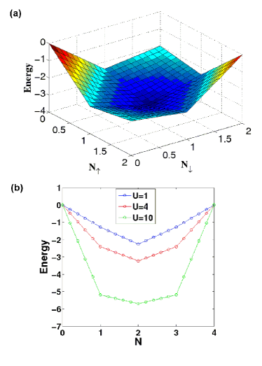
Figure 5: (Color online) (a) three-dimensional plot of the ground state energy as a function of $(N_{\uparrow},N_{\downarrow})$ for the symmetric case with $U=4$. (b) Ground state energy along the paramagnetic line in the symmetric case for several $U$-values. Energies are given in units of $|t|$.

We find that $Q$ is spin-degenerate only in regions 1 and 8 of Fig. 4, where $N$ is smaller than $1$, or bigger than $3$. However, we find that the spin-degeneracy is lifted if $1<N<3$, because here the interplay between kinetic energy and Coulomb interactions is more convoluted. The minima of $Q$ and $E^{0}$ occur now along the paramagnetic line $M=N_{\uparrow}-N_{\downarrow}=0$ regardless of the value of the on-site energy $\epsilon_{d}$, and of $U$. This is shown in Fig. 5(a), where the ground-state energy is plotted in the $(N_{\uparrow},N_{\downarrow})$-plane for the symmetric case and $U=4$. Here the characteristic polygonal shape as well as the presence/absence of spin degeneracies in the different regions are apparent. The position of the absolute minimum of $E^{0}$ along the paramagnetic line in contrast does depend on $\epsilon_{d}$ and on $U$. For the symmetric case, $\epsilon_{d}+U/2=0$, the minimum is placed at $N=2$. Fig. 5(b) shows $E^{0}$ as a function of $N$ along the paramagnetic line for the symmetric case and for several values of $U$ which cover the weak-, intermediate- and strong-coupling regimes of the model. The chemical potential and the energy value of the HOMO are given by the slope of these curves. They exhibit the expected discontinuous behavior at integer values of $N$Perdew82 ; Perdew83 ; Mori09 . Finally, it can be checked that this $Q$ functional renders the correct atomic limit by taking explicitly $t\rightarrow 0$ in Eq. (17). As a consequence the exact $Q$ functional is free from the delocalization error of mean-field theory. The analytic expressions for $Q$ enable to find the exact Exchange-correlation potentials for the two-site model $(V_{c,\sigma}^{XC}$, $V_{d,\sigma}^{XC})$. Notice that these potentials keep the full non-local dependence on occupations, because the potential at a given site $(i,\sigma)$ depends on all the densities $n_{j,\sigma^{\prime}}$. In contrast, it is very difficult to determine accurately the non-local terms by a numerical solution of this model, or by extending the Bethe ansatz LDA approach. We define the exact KS Hamiltonian for this double-site Anderson model as

$$H_{KS}=\sum_{i=(c,d),\sigma}(\epsilon_{i}\,+V_{i,\sigma}^{XC})\,\hat{n}_{i,\sigma}-t\,\sum_{\sigma}\,(\hat{c}_{\sigma}^{\dagger}\,\hat{d}_{\sigma}\,+\,\hat{d}_{\sigma}^{\dagger}\,\hat{c}_{\sigma}\,)-H_{dc}$$ (22)

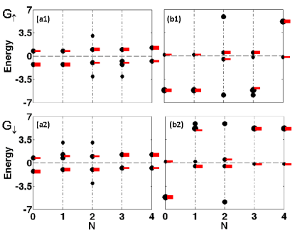
Figure 6: (Color online) Quasi-particle spectrum of the symmetric double-site Anderson model as a function of the electron number $N$, computed at the thick dots shown in Fig. 4. Green’s functions poles for $U=1$ ((a1) and (a2)) and $U=10$ ((b1) and (b2)). The upper and lower panels show $G_{d,\uparrow}$ and $G_{d,\downarrow}$, respectively. The energies of the many-body quasi-particles are shown as black dots whose width is proportional to the quasi-particle weight. the Kohn-Sham eigenstates are displayed as red dashes. The position of the one-particle HOMO level is marked by a thicker dash. Energies are given in units of $|t|$.

This Hamiltonian only has two KS eigenvalues per spin for all values of the physical parameters, which are discontinuous at integer $N_{\sigma}$-values. In other words, the numerical values of the KS eigenvalues are constant within each of the eight regions in Fig. 4, but differ from region to region. We compare now the KS eigenvalues with the exact many-body QP spectrum extracted from the poles of the many-body Green’s function at the impurity’s position. Notice again that only integer electron numbers $N=0,1,2,3,4$ have a physical meaning. For $N=1$, the system contains a single electron which must have either spin up or down. If a ground state wave-function with spin up $|\Psi_{1,\uparrow}>$ is chosen, then the spin-up and -down Green’s functions are different,

$$G_{d,\uparrow} = \frac{|<\Psi_{2,\uparrow,\uparrow}|\,c_{d,\uparrow}^{\dagger}\,|\Psi_{1,\uparrow}>|^{2}}{\omega+E_{1,\uparrow}-E_{2,\uparrow,\uparrow}+i\,\delta}+\frac{|<\Psi_{0}|\,c_{d,\uparrow}\,|\Psi_{1,\uparrow}^{1}>|^{2}}{\omega+E_{1,\uparrow}^{1}-E_{0}+i\,\delta}$$

$$G_{d,\downarrow} = \sum_{n}\frac{|<\Psi_{2}^{n}|\,c_{d,\downarrow}^{\dagger}\,|\Psi_{1,\uparrow}>|^{2}}{\omega+E_{1,\uparrow}^{1}-E_{2}^{n}+i\,\delta}$$ (23)

where the summation runs over all spin-0 states with $N=2$, and $\Psi_{2,\uparrow,\uparrow}$ indicate the spin-1 $N=2$ state. Similar words can be said for $N=3$. Romaniello and coworkersRomaniello09 have compared the spectrum of many-body QPs of this model with the poles of Green functions evaluated either in the GW approximation, or including vertex corrections. They have shown that the mean-field static correlation error is amended. However, even inclusion of vertex corrections does not allow to recover the QP spectrum in the atomic limit, showing how hard is to fully get rid of the delocalization error.

The exact KS Green’s function can be computed using the equations-of-motion method giving rise to the following expression

$$G_{d,\sigma}^{KS}=\frac{\omega-\epsilon_{c}-V_{c,\sigma}^{XC}}{(\omega-\epsilon_{c}-V_{c,\sigma}^{XC})\,(\omega-\epsilon_{d}-V_{d,\sigma}^{XC})-|t|^{2}}$$ (24)

This formula must be guided by the results obtained from the Lehmann representation at integer $N$. We compare now the poles of the many-body and exact KS Green’s functions by evaluating $V^{XC}$ at the points in the $(N_{\uparrow},N_{\downarrow})$ path shown in Fig. 4. This correspond to a paramagnetic solution for $N=2$ and a spin-up state for $N=1,3$. Fig. 6 shows the poles of $G$ and $G^{KS}$ as a function of the electron number $N$ for a symmetric case, and for values of $U$ in the weak- and strong-coupling regimes. The figure also shows which of the KS eigenvalues corresponds to the HOMO level. Notice that the exact many-body and KS spectra closely match for values of $U$ not only in the weakly-correlated, but also in the strongly-correlated regimes. However, extra many-body peaks appear at $N=1,2,3$, which are not provided by the exact KS Hamiltonian. In contrast, the number of many-body and KS QPs is the same for $N=0,4$ because an electron added to an empty system or a hole added to a fully occupied system can not Coulomb-interact with anything. Occupation $N=2$ corresponds to the strongly-correlated Kondo regime if $U$ is large, which is the case shown in Fig. 6(b). Here the many-body QP spectrum has four poles. These can be classified into two sets of peaks placed symmetrically about the zero-energy line. The first set is located around $\pm U/2$. The two peaks are separated by an energy of order $U$ and correspond to the upper and lower Hubbard bands. The second set develops into the Kondo resonance for more realistic models where ${\cal M}$ is made large. The KS spectrum has only two QP, which agree with the two Kondo-like many-body QPs. In other words, the KS spectrum shows no trace now of the lower and upper Hubbard band precursors. For $N=1$, the up-spin KS spectrum matches the many-body spectrum because the many-body phase-space for adding a spin-up electron or hole is very limited. However, the many-body phase-space for the addition of a spin-down electron is larger, which renders additional many-body spin-down quasi-electron peaks. Similar words can be said for $N=3$, where additional spin-up quasi-hole peaks are apparent. Notice in any case that the many-body and KS HOMO levels always agree with each other.

V Conclusions

We have presented analytic expressions for the exact density functionals of several simple models of strongly correlated electrons, from which we have obtained the exact ground-state energy. Those analytic expressions have allowed us to write down the full non-local dependence of $V^{XC}$ and KS Hamiltonians on the occupations. We have computed the exact KS eigenvalues and compared them with the true many-body QP, as obtained from the poles of the Green’s functions. We have shown with explicit examples that exact DFT preserves the quantum nature of electron-electron interactions, as opposed to mean-field theory and improvements over it as the GW approximation. It is also superior to more sophisticated perturbative approximations including vertex corrections. The exact functionals do not show any trace of self-interaction, static correlation, or delocalization errors.

We have found that the KS eigenvalues spectrum agrees to a large extent, but not fully, with the exact many-body spectrum. This is to say that all KS eigenvalues agree with some of the many-body QPs. However, the many-body QP spectrum is richer because the phase-space for addition of quasi-electrons or quasi-holes is larger. The exact functional only warrants the correct position of the HOMO level, while in general other KS eigenvalues may or may not agree with the exact many-body QP. Remarkably, we have found that the KS spectrum most possibly describes the Kondo peak in the Kondo regime. However, it is quite plausible that it won’t contain either the lower and upper Hubbard bands, or both. Exact DFT has similarities with the Renormalized Perturbation Theory proposed some time ago by HewsonHewson93 . The perturbative expansion shown in Eq. (2) would possibly describe the full many-body spectrum with simple approximations for the self-energy.

Appendix A Double-site Hubbard model

We use the following notation for the hamiltonian of the double-site Hubbard model

$$\hat{H}= \sum_{\sigma}\,\epsilon_{0}\,(\hat{n}_{1,\sigma}\,+\hat{n}_{2,\sigma})-\,t_{0}\,\sum_{\sigma}\,(\,\hat{c}_{1,\sigma}^{\dagger}\,\hat{c}_{2,\sigma}\,+\,\hat{c}_{2,\sigma}^{\dagger}\,\hat{c}_{1,\sigma}\,)\,+\,U\,\sum_{i=1,2}\hat{n}_{i,\uparrow}\,\hat{n}_{i,\downarrow}$$

The expressions for exact density functional are quite similar to those of the double-site Anderson model,

$$\begin{array}[]{lll}F_{1}&=&-\left[\,\sqrt{n_{1,\uparrow}\,n_{2,\uparrow}}+\sqrt{n_{1,\downarrow}\,n_{2,\downarrow}}\,\right]\\ \\ F_{2}&=&-\left[\,\sqrt{(1-n_{1}+x^{2}-y^{2})\,(1-n_{2}-x^{2}+y^{2})}+(x+y)\,(\sqrt{n_{1,\uparrow}-x^{2}}+\sqrt{n_{2,\uparrow}-y^{2}})\,\right]+U\,(x^{2}+y^{2})\\ \\ F_{3}&=&-\left[\,\sqrt{(n_{1,\uparrow}-x^{2}-z^{2})\,(1-n_{1}-n_{2,\downarrow}+x^{2}+z^{2})}+\sqrt{(n_{2,\downarrow}-y^{2}-z^{2})\,(1-n_{1,\uparrow}-n_{2}+y^{2}+z^{2})}\right.\\ &&+\left.(x+y)\,\left(z+\sqrt{n_{1}+n_{2}-1-x^{2}-y^{2}-z^{2}}\right)\right]+U\,(x^{2}+y^{2})\\ \\ F_{4}&=&-\left[\,\sqrt{(1-n_{1}+x^{2}-y^{2})\,(1-n_{2}-x^{2}+y^{2})}+(x+y)\,(\sqrt{n_{1,\downarrow}-x^{2}}+\sqrt{n_{2,\downarrow}-y^{2}})\,\right]+U\,(x^{2}+y^{2})\\ \\ F_{5}&=&-\left[\,\sqrt{(1-n_{1}+x^{2}-y^{2})\,(1-n_{2}-x^{2}+y^{2})}+(x+y)\,(\sqrt{1-n_{1,\downarrow}-y^{2}}+\sqrt{1-n_{2,\downarrow}-x^{2}})\,\right]\\ &&\,\,\,\,\,\,\,\,\,\,\,\,\,\,\,\,\,+U\,(n_{1}+n_{2}-2+x^{2}+y^{2})\\ \end{array}$$

$$\begin{array}[]{lll}F_{6}&=&-\left[\,\sqrt{(n_{1,\downarrow}-1+y^{2}+z^{2})\,(2-n_{1}-n_{2,\uparrow}-y^{2}-z^{2})}+\sqrt{(n_{2,\uparrow}-1+x^{2}+z^{2})\,(2-n_{1,\downarrow}-n_{2}-x^{2}-z^{2})}\right.\\ &&\,\,\,\,\,\,\,\,\,\,\,\,\,\,+\left.(x+y)\,\left(z+\sqrt{3-n_{1}-n_{2}-x^{2}-y^{2}-z^{2}}\right)\right]+U\,(n_{1}+n_{2}-2+x^{2}+y^{2})\\ \\ F_{7}&=&-\left[\,\sqrt{(1-n_{1}+x^{2}-y^{2})\,(1-n_{2}-x^{2}+y^{2})}+(x+y)\,(\sqrt{1-n_{1,\uparrow}-y^{2}}+\sqrt{1-n_{2,\uparrow}-x^{2}})\,\right]\\ &&\,\,\,\,\,\,\,\,\,\,\,\,\,\,\,\,\,+U\,(n_{1}+n_{2}-2+x^{2}+y^{2})\\ \\ F_{8}&=&-\left[\,\sqrt{(1-n_{1,\uparrow})\,(1-n_{2,\uparrow})}+\sqrt{(1-n_{1,\downarrow})\,(1-n_{2,\downarrow})}\,\right]+U\,(n_{1}+n_{2}-2)\end{array}$$

where the functionals $F_{a}$ are defined as

$$F_{a}=\frac{<\hat{H}>-(n_{1}+n_{2})\,\epsilon_{0}}{2|t_{0}|}$$

and where $Q$ is found by minimizing $F_{a}$ with respect to $x$ and $y$. Along the line $N_{\uparrow}+N_{\downarrow}=2$, the formulae for the $F$-functional can be simplified as follows:

$$F = -\left(\sqrt{n_{1,\downarrow}-x^{2}}+\sqrt{1-n_{2,\uparrow}-x^{2}}\right)\,\left(x+\sqrt{1-n_{1}+x^{2}}\right)+U\,(1-n_{1}+2x^{2})$$

$$= -\left(\sqrt{n_{1,\uparrow}-x^{2}}+\sqrt{1-n_{2,\downarrow}-x^{2}}\right)\,\left(x+\sqrt{1-n_{1}+x^{2}}\right)+U\,(1-n_{1}+2x^{2})$$

where the first equation is obeyed if $N_{\uparrow}>1$, $N_{\downarrow}<1$, and vice versa. $Q$ is now obtained by minimizing the above equation with respect to $x$.

Appendix B Double-site Anderson model

The full expressions for $F_{a}$ are as follows:

$$\begin{array}[]{lll}F_{1}&=&-\left[\,\sqrt{n_{c,\uparrow}\,n_{d,\uparrow}}+\sqrt{n_{c,\downarrow}\,n_{d,\downarrow}}\,\right]\\ \\ F_{2}&=&-\left[\,\sqrt{(1-n_{c}+x^{2}-y^{2})\,(1-n_{d}-x^{2}+y^{2})}+(x+y)\,(\sqrt{n_{c,\uparrow}-x^{2}}+\sqrt{n_{d,\uparrow}-y^{2}})\,\right]+U\,y^{2}\\ \\ F_{3}&=&-\left[\,\sqrt{(n_{c,\uparrow}-x^{2}-z^{2})\,(1-n_{c}-n_{d,\downarrow}+x^{2}+z^{2})}+\sqrt{(n_{d,\downarrow}-y^{2}-z^{2})\,(1-n_{c,\uparrow}-n_{d}+y^{2}+z^{2})}\right.\\ &&\,\,\,\,\,\,\,\,\,\,\,\,\,+\left.(x+y)\,\left(z+\sqrt{N-1-x^{2}-y^{2}-z^{2}}\right)\right]+U\,y^{2}\\ \\ F_{4}&=&-\left[\,\sqrt{(1-n_{c}+x^{2}-y^{2})\,(1-n_{d}-x^{2}+y^{2})}+(x+y)\,(\sqrt{n_{c,\downarrow}-x^{2}}+\sqrt{n_{d,\downarrow}-y^{2}})\,\right]+U\,y^{2}\\ \\ F_{5}&=&-\left[\,\sqrt{(1-n_{c}+x^{2}-y^{2})\,(1-n_{d}-x^{2}+y^{2})}+(x+y)\,(\sqrt{1-n_{c,\downarrow}-y^{2}}+\sqrt{1-n_{d,\downarrow}-x^{2}})\,\right.+U\,(n_{d}-1+x^{2})\\ \\ F_{6}&=&-\left[\,\sqrt{(n_{c,\downarrow}-1+y^{2}+z^{2})\,(2-n_{c}-n_{d,\uparrow}-y^{2}-z^{2})}+\sqrt{(n_{d,\uparrow}-1+x^{2}+z^{2})\,(2-n_{c,\downarrow}-n_{d}-x^{2}-z^{2})}\right.\\ &&\,\,\,\,\,\,\,\,\,\,\,\,\,\,\,\,\,+\left.(x+y)\,\left(z+\sqrt{3-N-x^{2}-y^{2}-z^{2}}\right)\right]+U\,(n_{d}-1+x^{2})\\ \\ F_{7}&=&-\left[\,\sqrt{(1-n_{c}+x^{2}-y^{2})\,(1-n_{d}-x^{2}+y^{2})}+(x+y)\,(\sqrt{1-n_{c,\uparrow}-y^{2}}+\sqrt{1-n_{d,\uparrow}-x^{2}})\,\right]+U\,(n_{d}-1+x^{2})\\ \\ F_{8}&=&-\left[\,\sqrt{(1-n_{c,\uparrow})\,(1-n_{d,\uparrow})}+\sqrt{(1-n_{c,\downarrow})\,(1-n_{d,\downarrow})}\,\right]+U\,(n_{d}-1)\end{array}$$ (25)

Q is again found by minimizing $F_{a}$ with respect to $x$ and $y$. Along the line $N_{\uparrow}+N_{\downarrow}=2$, the formulae for the $F$-functional can be simplified, and read as follows:

$$F = -\left(\sqrt{n_{c,\downarrow}-x^{2}}+\sqrt{1-n_{d,\uparrow}-x^{2}}\right)\,\left(x+\sqrt{1-n_{c}+x^{2}}\right)+U\,(n_{d}-1+x^{2})$$

$$= -\left(\sqrt{n_{c,\uparrow}-x^{2}}+\sqrt{1-n_{d,\downarrow}-x^{2}}\right)\,\left(x+\sqrt{1-n_{c}+x^{2}}\right)+U\,(n_{d}-1+x^{2})$$

where the first equation is obeyed if $N_{\uparrow}>1$, $N_{\downarrow}<1$, and vice versa. $Q$ is now obtained by minimizing the above equation with respect to $x$.

Appendix C M-site spinless fermion model

We show in this appendix the exact DFT solution of the double-site spinless fermion model, which corresponds to taking ${\cal M}=1$ and discarding the spin index in Eq. (1),

$$\hat{H}=\epsilon_{c}\,\hat{n}_{c}+\epsilon_{d}\,\hat{n}_{d}-t(\hat{c}^{\dagger}\,\hat{d}+\hat{d}^{\dagger}\,\hat{c})+U\hat{n}_{d}\,\hat{n}_{c}$$ (26)

We use a variational wave function of the form

$$|\,\phi>\,=\,a_{0}\,|\,0,0>\,+\,a_{c}\,|\,1,0>\,+\,a_{d}\,|\,0,1>\,+\,a_{cd}\,|\,1,1>$$ (27)

to find explicit formulae for the expectation values of $\hat{H}$ and $\hat{n}_{c}$, $\hat{n}_{d}$ as a function of the parameters $a_{i}$,

$$<\hat{H}> = \epsilon_{c}\,n_{c}+\epsilon_{d}\,n_{d}-2\,t\cos\varphi\,\,\frac{|a_{c}|\,|a_{d}|}{D}$$

$$<\hat{n}_{c}> = \frac{|a_{c}|^{2}\,+\,|a_{cd}|^{2}}{D}$$

$$<\hat{n}_{d}> = \frac{|a_{d}|^{2}\,+\,|a_{cd}|^{2}}{D}$$ (28)

$$D = |a_{0}|^{2}+|a_{c}|^{2}\,+|a_{d}|^{2}+|a_{cd}|^{2}$$

We solve for $|a_{c}|$, $|a_{d}|$ in the above equations for $n_{c,d}$ and substitute the result back in the equation for $<H>$. This yields the following expressions for $<\hat{H}>-\epsilon_{c}\,<\hat{n}_{c}>-\epsilon_{d}\,<\hat{n}_{d}>$

$$-2\,t\,cos\varphi\,\,\frac{\sqrt{n_{d}|a_{0}|^{2}+(n_{c}-1)|a_{cd}|^{2}}\,\,\sqrt{n_{c}|a_{0}|^{2}+(n_{d}-1)|a_{cd}|^{2}}}{|a_{0}|^{2}-|a_{cd}|^{2}}$$

$$-2\,t\,cos\varphi\,\,\frac{\sqrt{(1-n_{c})|a_{cd}|^{2}-n_{d}|a_{0}|^{2}}\,\,\sqrt{(1-n_{d})|a_{cd}|^{2}-n_{c}|a_{0}|^{2}}}{|a_{cd}|^{2}-|a_{0}|^{2}}$$ (29)

where the first and second line apply if $0<N<1$ or $1<N<2$, respectively. The energy functional $Q[n_{c},n_{d}]$ is found by minimizing the above expression with respect to $a_{0},a_{cd}$ and $\varphi$. The minimum of the functional happens when $a_{cd}=0$ for $0<N<1$, while for $1<N<2$, it is $a_{0}$ which vanishes. The resulting functional $Q[n_{c},n_{d}]-\epsilon_{c}\,n_{c}-\epsilon_{d}\,n_{d}\,$ has the following piece-wise shape:

$$- 2\,|t|\,\sqrt{n_{c}\,n_{d}}$$ (30)

$$- 2\,|t|\,\sqrt{(1-n_{c})\,(1-n_{d})}\,+\,U\,(n_{c}+n_{d}-1)$$

where again the first and second line apply if $0<N<1$ or $1<N<2$, respectively. $Q$ can be easily split into kinetic and interacting parts, where both must be defined piece-wise. The kinetic term explicitly shows electron-hole symmetry. The interacting term is non-zero only if $N>1$, from which a rather simple expression for the exact $V^{XC}$ can be extracted.

References

- (1) P. Hohenberg and W. Kohn, Phys. Rev. 136, B864 (1964).
- (2) W. Kohn and L. J. Sham, Phys. Rev. 140, A1133 (1965).
- (3) J. P. Perdew and A. Zunger, Phys. Rev. B 23, 5048 (1981).
- (4) J. P. Perdew, K. Burke, and M. Ernzerhof, Phys. Rev. Lett. 77, 3865 (1996).
- (5) A. D. Becke, J. Chem. Phys. 98, 1372 (1993).
- (6) A. J. Cohen, P. Mori-S�nchez and W. Yang, Science 321, 792 (2008).
- (7) P. Mori-Sánchez, A. J. Cohen and W. Yang, Phys. Rev. Lett. 102, 066403 (2009).
- (8) K. Schonhammer, O. Gunnarsson and R. M. Noack, Phys. Rev. B 52, 2504 (1995).
- (9) E. H. Lieb and F. Y. Wu, Phys. Rev. Lett. 20, 1445 (1968).
- (10) C. N. Yang and C. P. Yang, Phys. Rev. B 150, 321 (1966).
- (11) N. A. Lima, M. F. Silva, L. N. Oliveira and K. Capelle, Phys. Rev. Lett. 90, 146402 (2003).
- (12) S. Schenk, M. Dzierzawa, P. Schwab and U. Eckern, Phys. Rev. B 78, 165102 (2008).
- (13) C. Verdozzi, Phys. Rev. Lett. 101, 166401 (2008).
- (14) S. Kurth, G. Stefanucci, E. Khosravi, C. Verdozzi and E. K. U. Gross, Phys. Rev. Lett. 104, 236801 (2010).
- (15) J. P. Bergfield, Z. Liu, K. Burke and C. Stafford, arXiv:1106.3104v1
- (16) A. M. Tsvelick, P. B. Wiegmann, Adv. Phys. 32, 453 (1983).
- (17) J. F. Janak, Phys. Rev. B 18, 7165 (1978).
- (18) J. P. Perdew and M. Levy, Phys. Rev. Lett. 51, 1884 (1983).
- (19) L. J. Sham and M. Schluter, Phys. Rev. Lett. 51, 1888 (1983).
- (20) P. Romaniello, S. Guyot and L. Reining, J. Chem. Phys. 131, 154111 (2009).
- (21) Notice that the added quasi-electron will have two excitation energies. The first will appear if it falls in the same atom where the first electron was placed since it will feel the mutual Coulomb interaction. The second excitation energy will appear if it falls in the empty atom, because then it will feel no Coulomb interaction at all. In contrast, mean field theory only gives a single excitation energy because the added electron will interact with half an electron regardless of the atom where it falls.
- (22) M. M. Rieger and P. Vogl, Phys. Rev. B 52, 16567 (1995).
- (23) A. Filippetti and N. A. Spaldin, Phys. Rev. B 67, 125109 (2003).
- (24) C. Toher, A. Filippetti, S. Sanvito, and K. Burke, Phys. Rev. Lett. 95, 146402 (2005)
- (25) L. Hedin, Phys. Rev. 139, A796 (1965).
- (26) W. G. Aulbur, L. Johnson and J. W. Wilkins, Solid State Physics 54, 1 (1999).
- (27) G. Onida, L. Reining and A. Rubio, Rev. Mod. Phys. 74, 601 (2002).
- (28) F. Bruneval, F. Sottile, V. Olevano, R. Del Sole and L. Reining, Phys. Rev. Lett. 94, 186402 (2005).
- (29) X. Wang, C. D. Spataru, M. S. Hybertsen and A. J. Millis, Phys. Rev. B 77, 045119 (2008).
- (30) K. S. Thygesen and A. Rubio, Phys. Rev. B 77, 115333 (2008).
- (31) A. C. Hewson, The Kondo Problem to Heavy Fermions (Cambridge University Press, Cambridge, 1992).
- (32) J. Ferrer, A. Martin-Rodero and F. Flores, Phys. Rev. B 36, 6149 (1987).
- (33) P. S. Sun and G. Kotliar, Phys. Rev. Lett. 92, 196402 (2004).
- (34) G. Kotliar, S. Y. Savrasov, K. Haule, V. S. Oudovenko, O. Parcollet, C. A. Marianetti, Rev. Mod. Phsy. 78, 866 (2006).
- (35) D. Jacob, K. Haule and G. Kotliar, Phys. Rev. B 82, 195115 (2010).
- (36) R. Korytar and N. Lorente, J. Phys.: Condens. Matter 23, 355009 (2011).
- (37) E.M. Stoudenmire, L. O. Wagner, S. R. White and K. Burke, arXiv:1107.2394v1
- (38) M. Levy, Proc. Natl. Acad. Sci. U.S.A. 76, 6062 (1979).
- (39) The minimization procedure described in the main text could be applied even in the hypothetical case where there would exist several degenerate states within a given box, by just choosing one of these as a representative of the box.
- (40) G. D. Mahan, Many Particle Physics (Plenum Publishing Corporation, 1981).
- (41) L. P. Kadanoff and G. Baym, Quantum Statistical Mechanics (Addison-Wesley Publishing Company, 1962)
- (42) O. V. Gritsenko and E. J. Baerends, Phys. Rev. A 54, 1957 (1996).
- (43) N. Helbig, I. V. Tokatly and A. Rubio, J. Chem. Phys. 131, 224105 (2009).
- (44) J. P. Perdew, R. G. Parr, M. Levy and J. L. Balduz, Phys. Rev. Lett. 49, 1691 (1982).
- (45) A. C. Hewson, Phys. Rev. Lett. 70, 4007 (1993).