New numerical results and novel effective string predictions for Wilson loops

Abstract:

We compute the prediction of the Nambu-Goto effective string model for a rectangular Wilson loop up to three loops. This is done through the use of an operatorial, first order formulation and of the open string analogues of boundary states. This result is interesting since there are universality theorems stating that the predictions up to three loops are common to all effective string models. To test the effective string prediction, we use the Montecarlo evaluation, in the 3d Ising gauge model, of an observable (the ratio of two Wilson loops with the same perimeter) for which boundary effects are relatively small. Our simulation attains a level of precision which is sufficient to test the two-loop correction. The three-loop correction seems to go in the right direction, but is actually yet beyond the reach of our simulation, since its effect is comparable with the statistical errors of the latter.

1 Introduction

The proposal that the strong-coupling dynamics of gauge theories could be captured by an effective string theory is a long-standing one [1]-[10]; the fluctuating long string, in this approach, is the color flux tube joining coloured charges. Perhaps the most direct prediction that can be extracted from the effective string is the shape of the potential $V(R)$ between two external sources (two static quarks) at distance $R$. From the gauge theory point of view, if we have a rectangular Wilson loop $W(L,R)$ of sides $L$ and $R$, the inter-quark potential is

$$V(R)=-\lim_{L\to\infty}\frac{1}{L}\log W(L,R)~{}.$$ (1)

In the confining phase, the area law for the Wilson loop corresponds to a linear potential

$$V(R)=\sigma R+\ldots~{}.$$ (2)

In a string interpretation, the area term $\sigma LR$ in the exponent of the Wilson loop is the classical action of an effective string model. Another way of measuring the static $q\bar{q}$ potential is to consider the correlator of two Polyakov loops at distance $R$ in a gauge theory at finite temperature $\propto 1/L$; in the strong-coupling regime, the string world-sheet describing this situation is a cylinder.

The simplest and most obvious choice for the effective string is the Nambu-Goto one [11, 12], where the action is the induced area of the string world-sheet, see eq. (5) below, and the degrees of freedom are the $D=d-2$ transverse fields. The action is non linear and contains, besides the kinetic term, a series of higher derivative interactions. Quantization is implemented by functional integration and can be carried out perturbatively. This approach was used in [13] to compute, up to two loop order, the string vacuum amplitude on world-sheets with disk, cylinder or torus topology (the first two being relevant for Wilson loops and Polyakov loop correlators respectively).

On general grounds, one expects any effective theory for a long string to contain as degrees of freedom the transverse fields, representing the Goldstone modes for the translational invariance broken by the string configuration. The “one loop” quantum corrections are then given by the functional determinants of the kinetic operators for the transverse modes and are the same for all effective models. They lead to the correction to the static potential known as “Lüscher term” [9, 10]:

$$V(R)=\sigma R-\frac{D\pi}{24R}+\ldots~{}.$$ (3)

Over the years, computer simulations of Polyakov loop correlators and Wilson loops have shown with increasing evidence the presence of this correction (for an up to date review see [14]), confirming the soundness of the effective string approach.

The various possible effective theories are distinguished by the form of their interaction terms, which in turn affect the perturbative corrections to the amplitudes, starting at two loops. The interaction terms cannot, however, be completely arbitrary. In [15] it was shown that the requirement that the effective string cylinder partition function (corresponding to a Polyakov loop correlator) can be re-expressed in terms of propagating closed string states fixes the coefficients of the first higher derivative terms. Moreover, if the effective string is supposed to describe the low-energy regime of a consistent quantum field theory, the Poincaré symmetry of the latter must be still realized. Since the configuration around which the long string fluctuates spontaneously breaks, in particular, the Lorentz transformations mixing longitudinal and transverse coordinates, these must be realized non-linearly in the effective action. This requirement is present in the analysis of [15], see [16], but was made more explicit and pursued further in [17]-[19], where it is shown that the coefficients of the quartic and sextic derivative interaction terms are almost completely fixed by this constraint, both for closed and open strings, and coincide with those of the NG model. This ”universality” of the lowest interaction terms suggests that Montecarlo simulations should be compatible with NG prediction also beyond the one-loop level.

Testing the effective string predictions beyond the one-loop terms, for instance by looking at subleading terms in the $1/R$ expansion of the effective potential, is a very serious challenge. It is a challenge from the computational point of view, because it requires to carry out simulations so precise as to distinguish deviations of the results from the one-loop predictions. However, thanks to the development of new algorithms and the surge in available computer power, such a precision is basically within reach. In particular, in the case of the three dimensional gauge Ising model in which, exploiting duality, high precision can be reached at a reasonable computational cost, universality was unambiguously confirmed at two loop level both in the case of the torus geometry [20, 21, 22] and in the case of the cylinder geometry [23, 24]. Testing universality at three loop level turned out to be more difficult. The only existing tests [25] were performed in very asymmetric geometries were string effects are magnified but systematic errors, due for instance to the vicinity of the deconfinement transition, are more difficult to control. For a survey of most recent results for other gauge groups or other observables see [14]). Until now no attempt to go beyond the one loop results was performed in the case of the disk geometry. Filling this gap is one of the main goals of the present paper.

Also on the theoretical side, extracting the higher loop effects of the effective string model is not an easy task. The diagrammatic evaluation of the effective string amplitudes carried out in [13] was pushed up to three loops, and extended to a generic effective string action to this order in [17], for the cylinder partition function only.

In this work, we derive higher loop corrections in the Nambu-Goto disk amplitude corresponding to the Wilson loop. Our method, which allows in fact to obtain the exact amplitude that resums the loop expansion, is based on the the first-order reformulation of the Nambu-Goto string model; it has already been successfully applied to the cylinder [26] and the torus [27, 28] partition functions. We will see that the Wilson loop case is more delicate, but we propose an exact expression which reproduces, at two-loop, the result of [13]: this represents a very non-trivial check and we trust therefore our results also to higher loops.

The universality of the first terms in the derivative expansion of the effective action explains why the NG model represents a good approximation of the correct effective string theory for the flux tube; in turn, testing NG to the order to which its effects are universal would represent a stringent test of the whole effective string approach.

Still, the NG model can not be the right one, and deviations from its predictions, when precisely identified, may help in the quest for the correct effective string. In particular, the Lorentz invariance should be preserved also at the quantum level. The quantum consistency of the NG theory is usually investigated by using a first-order re-formulation, which involves an independent metric on the world-sheet but is quadratic in the string fields: employing the Weyl invariance to reach the so-called ”conformal gauge”, the world-sheet metric decouples and one is left with a quadratic action, to be supplemented with the Virasoro constraints. This is the standard approach described in string theory textbooks, see for instance [29, 30]. The residual conformal invariance generated by the modes of the Virasoro constraints can be exploited to fix a light-cone (physical) gauge where only the $D$ transverse fields are independent; it can also be enforced, in the “covariant quantization”, by taking into account the effects of the ghost/anti-ghost system that arise from the Jacobian to fix the conformal gauge. In the light-cone gauge, the closure of the target-space Lorentz algebra at the quantum level requires $D=24$; however, when the string fluctuates around a long string configuration with length scale $R$, this anomaly is suppressed in the large $R$ limit [31]. In covariant quantization, the central charge $c_{\mathrm{gh}}=-26$ of the ghost/anti-ghost system has to be compensated by that of $D+2=26$ bosonic fields.

Polyakov’s approach [32] of functionally integrating over the intrinsic metric shows that for $D\not=26$ the scale of this metric does not decouple and represents an additional degree of freedom that has to be taken into account to ensure quantum consistency. This world-sheet boson is usually referred to as the Liouville field since its action is of the Liouville type. If the effective string theory must contain just the $D$ transverse d.o.f., and realize also at the quantum level the Lorentz algebra, none of the standard quantizations can thus be correct. An interesting proposal was put forward by Polchinski and Strominger in [33]; to reconcile the requirement of critical central charge with having just the $D$ transverse degrees of freedom, they proposed a Polyakov model where the Liouville field is re-expressed in terms of the induced metric, i.e., in terms of the transverse fields. The action becomes non-local, but admits nevertheless a sensible expansion around long string configurations. It has been shown that the first terms in the derivative expansion of this model agree with the NG ones, in accordance with the universality arguments. It seems however difficult to compute higher loop corrections to the amplitudes in this model.

Recently, some particular, supersymmetric, gauge theories have been finally given an explicit realization in terms of strings propagating on a curved manifold with an extra dimension, in the so-called AdS/CFT duality [34, 35, 36]; the extra dimension can be interpreted in terms of the energy scale [37] and as such it does not represent a spurious degree of freedom. From the point of view of the effective action for the transverse fields, the interaction terms would take into account the curved geometry. This is of course a very intriguing possibility.

There is an extra issue in devising the correct effective string action, namely the possible presence of boundary terms. Lattice simulations have made it clear that the Wilson loop expectation value displays, beside the leading area term, a perimeter term with an independent coupling:

$$W(L,R)\sim\exp\left(-\sigma LR-\mu(L+R)+\ldots\right)~{}.$$ (4)

In this paper, we will study a particular observable, corresponding to the ratio of two different rectangular Wilson loops, such that the leading perimeter dependence described in eq. (4) cancels [38]. However, it is natural to expect that the perimeter term is only the classical value of some boundary component of the effective action which also yields other, subleading, corrections to the amplitudes. In [15, 18, 19] the first few possible boundary terms in a derivative expansion of the effective action have been investigated for the Polyakov loop geometry, finding that they can lead to corrections of the order of $1/R^{4}$ ($R$ being the distance between the Polyakov loops); to our knowledge, no explicit evaluation of the effect of boundary terms in the Wilson loop geometry is available. From the theoretical point of view, in [39]-[43] by considering Polyakov quantization in presence of boundaries, it was found that boundary terms in the world-sheet actions are needed, and in particular a term proportional to the induced length of the boundary, whose leading contribution to the Wilson loop amplitude would indeed be a perimeter term. It would be nice to investigate the modifications of the Nambu-Goto calculations in presence of such a term, but we leave this to future work.

In comparing the outcomes of our simulations to the theoretical predictions of the Nambu-Goto effective model, we will have to take into account the likely presence of boundary terms, of which no explicit evaluation is available; this increases the uncertainties in the comparison.

As mentioned above the main goal of this paper was to compare theoretical predictions and Montecarlo simulations beyond one loop in the case of the Wilson loop geometry. We shall show that, using duality based algorithms, it is possible to study Wilson loops large enough to make boundary effects negligible and at the same time to reach a precision high enough to disentangle effective string corrections beyond the one loop level. As in the cases of the torus and cylinder geometry, we shall be able to confirm universality at the two loops level. The third loop corrections seem to go in the right direction, but their magnitude is of the same order as the statistical errors, so that they remain beyond the reach of present simulations.

2 Two-loop effective string prediction

In this section we summarize the two-loop prediction for the Wilson loop amplitude obtained in the Nambu-Goto effective string model. As discussed in the introduction, the predictions up to three loops are actually universal for all effective string models.

In the Nambu-Goto approach [11, 12] the action for the fluctuating surface spanned by the flux tube is simply its induced area in the $d$-dimensional target space:

$$S=\sigma\int d^{2}\xi\sqrt{\det g}~{},\hskip 17.07182ptg_{\alpha\beta}=\frac{\partial X^{M}}{\partial\xi^{\alpha}}\frac{\partial X^{N}}{\partial\xi^{\beta}}G_{MN}~{}.$$ (5)

Here $\sigma$ is the string tension, the surface is parametrized by proper coordinates $\xi^{\alpha}$, and $X^{M}(\xi)$ ($M=1,\ldots,D+2$) describe the target space position of a point specified by $\xi$. For us the target space metric $G_{MN}$ will always be the flat one. Our analysis aims at comparing effective string predictions with lattice simulations of gauge theories, which are always performed with an Euclidean time. As a consequence, we use the Euclidean signature on the target space as well as on the world-sheet; this is what is commonly done in the literature about the effective string approach

Consider a rectangular Wilson loop of sides $L$ and $R$ in the $x^{1},x^{2}$ plane. The direction $x^{1}$ is interpreted as the Euclidean time, so that in the limit $L\to\infty$ one can extract the static quark-antiquark potential via eq. (1) and compare it directly with lattice simulations.

In the so-called “static” gauge the proper coordinates of the string are identified with $x^{1}$ and $x^{2}$ already at the classical level. The partition function for the Wilson loop surface is then obtained by functional integration over the transverse fields $\vec{X}(x^{1},x^{2})$:

$$W(L,R) =\int D\vec{X}\,\exp\left\{-\sigma\int_{0}^{L}dx^{1}\int_{0}^{R}dx^{2}\left(1+(\partial_{1}\vec{X})^{2}+(\partial_{2}\vec{X})^{2}+(\partial_{1}\vec{X}\wedge\partial_{2}\vec{X})^{2}\right)^{\frac{1}{2}}\right\}$$ (6)

$$=\int D\vec{X}\,\exp\left\{-\sigma\int_{0}^{L}dx^{1}\int_{0}^{R}dx^{2}\left[1+\frac{1}{2}(\partial_{1}\vec{X})^{2}+\frac{1}{2}(\partial_{2}\vec{X})^{2}+\mbox{interactions}\right]\right\}~{},$$

with the transverse fields $\vec{X}$ vanishing on the Wilson loop perimeter. To this NG action, terms living on the boundary of the domain can (and must) be added, and their effect is expected to be important, especially for small loops. In this paper, however, we will not deal explicitly with the quantum corrections induced by such terms. Eq. 6 describes a statistical sum over surfaces bounded by the Wilson loop.

By construction, we must have

$$W(L,R)=W(R,L)~{}.$$ (7)

Expanding the square root as in the second line of eq. (6), the constant term leads to the well-known classical area law

$$W_{\mathrm{cl}}(R,L)=\mathrm{e}^{-\sigma RL+p(R+L)+k}~{}.$$ (8)

Here on top of the area law we have included a perimeter term, whose strength is parametrized by $p$, which arises from boundary terms in the action. The overall normalization, which is out of control, is parametrized by $k$.

From the functional integration over the fields $\vec{X}$, with the bulk action given in the second line of eq. (6), one gets the determinant of their kinetic operator multiplied by perturbative corrections, starting at two loops. The result has the structure

$$W(L,R)=\mathrm{e}^{-\sigma\mathcal{A}+p(R+L)+k}\,\left(\frac{\eta(\mathrm{i}u)}{\sqrt{R}}\right)^{-\frac{D}{2}}\left\{1+\frac{\mathcal{L}_{2}(u)}{\sigma\mathcal{A}}+\frac{\mathcal{L}_{3}(u)}{(\sigma\mathcal{A})^{2}}+\ldots\right\}~{},$$ (9)

where, for ease of notation, we have introduced

$$\mathcal{A}=RL~{},~{}~{}~{}u=\frac{L}{R}~{}.$$ (10)

In eq. (9), the term $(\eta(\mathrm{i}u)/\sqrt{R})^{D/2}$, where by $\eta$ we denote Dedekind’s function (see Appendix A for relevant notation and definitions) is the functional determinant; it is invariant under $R\leftrightarrow L$, i.e., under $u\leftrightarrow 1/u$, as it follows from the modular transformation properties of the $\eta$ function. The corresponding contribution to the interquark potential of eq. (1) is the celebrated Lüscher term $D\pi/(24R)$ appearing in eq. (3) that represents the leading correction to the linear confining potential [9, 10].

With the impressive enhancement in precision of Montecarlo simulations in the last years and, above all, in view of the universality theorems discussed in the introduction it becomes important to evaluate and test also the subleading terms in eq. (9). The terms $\mathcal{L}_{a}(\mathrm{i}u)$ represent the corrections at order $a$ in the loop expansion parameter $\sigma\mathcal{A}$; they must be invariant under $u\leftrightarrow 1/u$.

The computation of the two-loop correction $\mathcal{L}_{2}$ was carried out almost 30 years ago by Dietz and Filk [13]. However, the two-loop result of [13] appears to be incompatible with the data obtained with various simulation techniques, see [44] for an account of recent attempts in this direction. This fact prompted us to a critical re-examination of the Dietz and Filk calculation. We found a mistake in their eq. (3.3). The correct result is

$$\mathcal{L}_{2}(u)=\left(\frac{\pi}{24}\right)^{2}\left[2D\,u^{2}E_{4}\left(\mathrm{i}u\right)-\frac{D(D-4)}{2}E_{2}\left(\mathrm{i}u\right)E_{2}\left(\mathrm{i}/u\right)\right]~{}.$$ (11)

where $E_{2}$ and $E_{4}$ denote the second and fourth order Eisenstein series, see Appendix A. We shall show in the next section that eq. (11) turns out to be compatible with the Montecarlo results, in accordance with its universal character.

3 New numerical results

In this section we compare the two-loops effective string prediction for Wilson loops with a set of numerical data extracted from a Montecarlo simulation of a suitable observable in the three-dimensional $\mathbb{Z}_{2}$ gauge model.

3.1 Definition of the observable in the 3d $\mathbb{Z}_{2}$ gauge model

The 3d $\mathbb{Z}_{2}$ gauge model on a cubic lattice is defined by the partition function

$$Z_{g}(\beta)=\sum_{\sigma_{l}=\pm 1}\exp\{-\beta S_{g}\}~{}.$$ (12)

The action $S_{g}$ is a sum over all the plaquettes of the lattice,

$$S_{g}=-\sum_{\Box}\sigma_{\Box}~{},~{}~{}~{}\sigma_{\Box}=\sigma_{l_{1}}\sigma_{l_{2}}\sigma_{l_{3}}\sigma_{l_{4}}~{},$$ (13)

where $\sigma_{l}$ are Ising variables located on the links of the lattice. This gauge model is equivalent to the standard Ising model by the Kramers-Wannier duality transformation

$$Z_{g}(\beta) \propto Z_{s}(\tilde{\beta})~{},$$ (14)

$$\tilde{\beta} =-\frac{1}{2}\log[\tanh(\beta)]~{},$$ (15)

where $Z_{s}$ is the partition function of the Ising model in the dual lattice

$$Z_{s}(\tilde{\beta})=\sum_{s_{i}=\pm 1}\exp\{-\tilde{\beta}H_{1}(s)\}~{}.$$ (16)

Here

$$H_{1}(s)=-\sum_{\langle ij\rangle}J_{\langle ij\rangle}s_{i}s_{j}$$ (17)

with $i$ and $j$ denoting the nodes of the dual lattice and the sum is over all the links $\langle ij\rangle$ of the dual lattice. Here the couplings $J_{ij}$ are fixed to the value $+1$ for all the links. This define a one-to-one mapping between the free energy densities in the thermodynamic limit. The dual of the Wilson loop expectation value , in which we are interested, is given by

$$W(R,L)=\frac{Z_{s,W}(\tilde{\beta})}{Z_{s}(\tilde{\beta})}~{},$$ (18)

where in $Z_{s,W}$ all the couplings of the links that intersect the surface $S$ enclosed by the Wilson loop take the value $J_{\langle ij\rangle}=-1$.

The form of the functional dependence of the Wilson loop on the sides $R,L$ is given in eq. (9), where we have to fix $D=d-2=1$. The values of the parameters $\sigma$,$p$ and $k$ appearing in the classical part of this expression are not predicted by the effective string theory. However $p$ and $k$ can be eliminated by considering ratios of Wilson loops with the same perimeter [38], as the ones of fig. 1. We will therefore consider the observable

$$R_{\mathrm{w}}(L,R,n)=\frac{W(L,R)}{W(L+n,R-n)}~{}.$$ (19)

Figure 1: The observable $R_{\mathrm{w}}(L,R,n)$ is given by the ratio of the Wilson loops $W(L,R)$ and $W(L+n,R-n)$.

3.2 Algorithm and simulation settings

In general, computing large Wilson loops is a difficult task because the Wilson loop expectation value decreases exponentially with the area, so the relative error increases exponentially. This is true also for the gauge Ising model but in this case, if one evaluates the dual observable eq.(18), the problem can be overcome. Our approach is essentially the same described in great detail in [23], adapted to the observable 19. In order to compute eq. (19) we factorize the ratio as follows:

$$R_{\mathrm{w}}(L,R,n)=\frac{W(L,R)}{W(L+1,R)}\frac{W(L+1,R)}{W(L+2,R)}\dots\frac{W(L+n,R)}{W(L+n,R-1)}\dots\frac{W(L+n,R-n+1)}{W(L+n,R-n)}$$ (20)

Every ratio of eq. (20) is then simulated separately, using a hierarchical algorithm as explained in [23].

In order to compare the effective string theory prediction with the numerical data we need a very precise estimate of the zero temperature string tension. We choose to simulate the model at coupling $\beta=0.75180$, for which the string tension is known with very high precision [45] to be $\sigma=0.0105241(15)$. We performed our simulations on a lattice of size $64\times 120\times 120$ and measured only Wilson loops lying along the directions of size $120$. The lattice sizes were chosen large enough to avoid finite size effects; in particular, we carefully tested that a lattice size of $64$ lattice spacings in the transverse direction was enough to avoid finite size corrections even for the largest loops that we studied.

3.3 Comparing the results to the two-loop predictions

We extracted from the simulation the ratio of expectation values

$$R_{\mathrm{w}}(L,\frac{L}{u},n)=\frac{W(L,\frac{L}{u})}{W(L+n,\frac{L}{u}-n)}$$ (21)

for different values of the asymmetry parameter $u=L/R>1$ and of $n$. The numerical results of the simulation are reported in Table (1). The leading classical behaviour of the observable $R_{\mathrm{w}}(L,L/u,n)$ is given by

$$R_{\mathrm{w}}(L,\frac{L}{u},n)=\exp\left\{-\sigma n\left(n+L(1-\frac{1}{u})\right)\right\}.$$ (22)

In order to isolate the quantum corrections in which we are interested, exploiting the fact that $\sigma$ is known with very high precision, we define the new observable

$$R_{\mathrm{w}}^{{}^{\prime}}(L,\frac{L}{u},n)=R_{\mathrm{w}}(L,\frac{L}{u},n)-\exp\left\{-\sigma n\left(n+L(1-\frac{1}{u})\right)\right\}~{}.$$ (23)

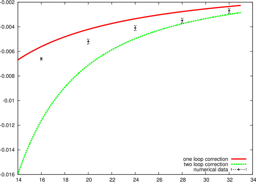
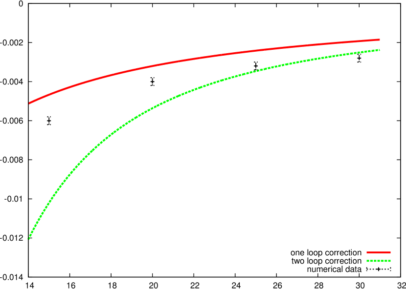
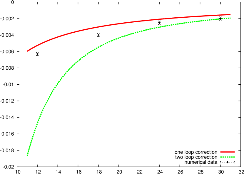
$R_{\mathrm{w}}^{{}^{\prime}}(L,\frac{3}{4}L,1)$	$R_{\mathrm{w}}^{{}^{\prime}}(L,\frac{4}{5}L,1)$
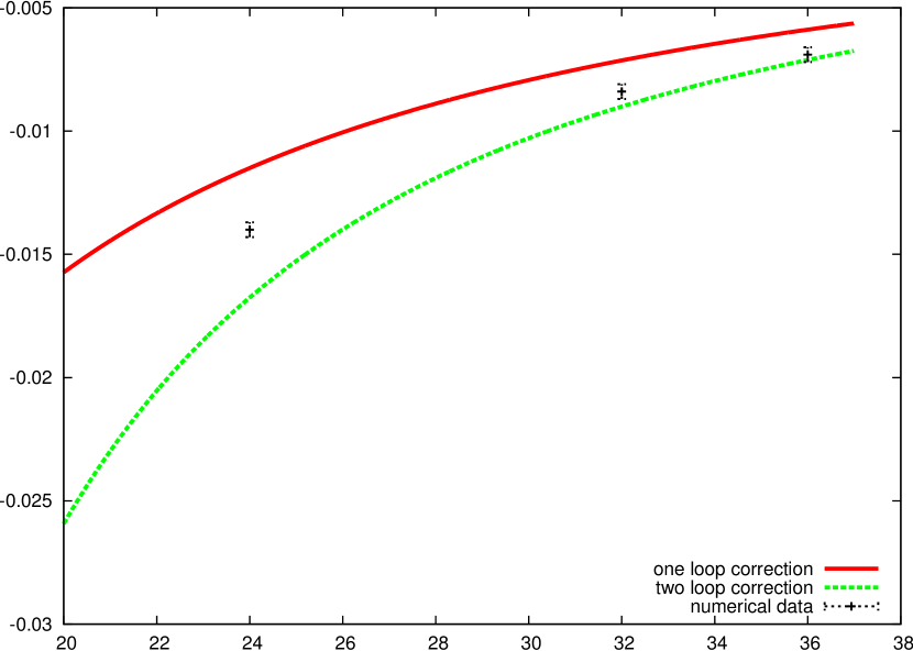
$R_{\mathrm{w}}^{{}^{\prime}}(L,\frac{5}{6}L,1)$	$R_{\mathrm{w}}^{{}^{\prime}}(L,\frac{3}{4}L,3)$

Figure 2: Plot of $R_{\mathrm{w}}^{{}^{\prime}}(L,L/u,n)$ for different values of $u$ and $n$ against the quantum string corrections, up to two loop. Note that the classical string prediction is $R_{\mathrm{w}}^{{}^{\prime}}=0$, see eq.s (22,23).

We plot in fig. (2) our data for $R_{\mathrm{w}}^{{}^{\prime}}$ against the quantum string corrections up to two loop. Looking at these figures we see that a few interesting facts emerge.

1. The deviation from the classical behavior $R_{\mathrm{w}}^{{}^{\prime}}=0$ is immediately visible from the plots: string corrections do definitely affect the Wilson loop ratio.

2. The deviation of the data is systematically larger than the one loop prediction (which is indicated by the full line in fig.2). For large enough values of $R$, the smallest of the two sides of the Wilson loop, the data converge toward the two loop string correction (the dashed line in fig.2) and for the largest values of $L$ we considered ($R>20$) they agree with it within the errors.

3. This agreement becomes worse as $R$ decreases. This also happens for values of $R$ much larger than the flux tube thickness and thus cannot be due to the breaking of the effective string picture. The most probable reason is the presence of subleading effects due to boundary terms in the effective string action.

The first point is a well established result: effective string corrections for the Wilson loop were observed for the first time in the gauge Ising model in [38] and later also in several other LGTs and in particular in the - physically relevant - four dimensional SU(3) LGT [46]. The second point, instead, is a new result in the Wilson loop geometry.

Let us address in more detail the third point. At present there is no explicit evaluation for the quantum effects due to boundary terms in the Wilson loop geometry. This is a very interesting and non trivial issue which we plan to address in future work. However, extrapolating to the Wilson case the existing results [19, 47] for the cylinder geometry we expect that these corrections should decrease at least as $1/R^{4}$. This behaviour seems indeed to fit rather well the deviations observed in fig.2. Extrapolating the fits to larger values of $R$ one can show that for $R>20$ boundary corrections are fully negligible. This statement holds true assuming for the boundary corrections any possible decreasing behaviour of the type $1/R^{n}$ with $n\geq 4$, assuming any value, compatible with the data at low $R$, for the amplitude of the correction and, most importantly, making no assumptions on the effective string corrections, except for those implied by the universality theorems.

This makes us confident that our results for the largest values of $R$ can be used for an unbiased test of our theoretical predictions. In this respect it is interesting to observe that in this region our data suggest that the universal three loop correction should be small or should have the opposite sign with respect to the two loop one. In order to clarify this point, however, we need to compute this correction. This is the main goal of the following section.

——- $L$ $R_{\mathrm{w}}(L,\frac{3}{4}L,1)$ $L$ $R_{\mathrm{w}}(L,\frac{4}{5}L,1)$ $L$ $R_{\mathrm{w}}(L,\frac{5}{6}L,1)$ $L$ $R_{\mathrm{w}}(L,\frac{3}{4}L,3)$ 16 0.9421(1) 15 0.9528(2) 12 0.9626(1) 24 0.7387(3) 20 0.9336(2) 20 0.9447(2) 18 0.9548(2) 32 0.6982(3) 24 0.9249(2) 25 0.9356(2) 24 0.9462(2) 36 0.6777(3) 28 0.9158(2) 30 0.9262(2) 30 0.9368(2) 32 0.9069(2) ——-

Table 1: Results for $R_{\mathrm{w}}^{{}^{\prime}}(L,R,n)$ as a function of the long side of the loop, for various fixed values of the ratio $u=L/R$ and of $n$.

4 Beyond two-loops: operatorial approach

Having argued that it is desirable to compute the three loop correction to the Wilson loop amplitude in the NG model, we proceed now to do so by resorting to an approach based on the first order re-formulation of the model itself. This approach has been used in [26] and [27] for the cylinder and torus partition functions respectively. The reasons to take this route are two-fold. On the one hand, carrying out the derivation of the three loop effect in the physical gauge by extending the two-loop computations of [13] is a daunting task. On the other hand, the application of the operatorial, first-order formalism to the Wilson loop disk partition function is not difficult but also not trivial and, as we will see, relies on the use of the rather non-standard (but perfectly sensible) concept of open string boundary states introduced in [48]. The way in which the loop expansion of the Wilson loop amplitude emerges in this formalism is quite interesting.

We use the first order formulation, requiring the introduction of an independent world-sheet metric $\gamma_{ab}$. This metric can then be gauge-fixed exploiting reparametrization invariance, and the open string action in the conformal gauge reads simply

$$S=\sigma\int d\xi^{1}\int_{0}^{\pi}d\xi^{2}\,\left[\left(\partial_{\xi^{1}}X^{M}\right)^{2}+\left(\partial_{\xi^{2}}X^{M}\right)^{2}\right]+S_{\mathrm{gh.}}~{},$$ (24)

where $\xi^{2}\in[0,\pi]$ parametrizes the spatial extension of the string and $\xi^{1}$ its proper (euclidean) time evolution. The fields $X^{M}(\xi^{1},\xi^{2})$, with $M=1,\ldots,D+2$, describe the embedding of the string world-sheet in the euclidean target space and form the 2-dimensional CFT of $D+2$ free bosons. The term $S_{\mathrm{gh.}}$ in eq. (24) is the action for the ghost and anti-ghost fields that arise from the Jacobian for fixing the conformal gauge. We do not really need here its explicit expression, see [29] or [30] for reviews.

We can treat this theory in an “Hamiltonian” way, by selecting the coordinate $\xi^{1}$ as a (radial, euclidean) “time” coordinate. At fixed $\xi^{1}$, the fields $X^{M}$ describe the embedding of the string in the target space; evolving in $\xi^{1}$ the string sweeps out a surface.

4.1 The Dirichlet string

We argue that such an operatorial description is possible also with the boundary conditions corresponding to a rectangular Wilson loop, as described in Fig. 3. We arbitrarily select one of the directions along the Wilson loop, say $x^{1}$, and regard the sides of the loop along which $x^{1}$ varies, which sit at distance $R$ in the $x^{2}$ direction, as the quark and anti-quark lines. Consider a open string whose end-points are attached to these two lines and are free to move in the $x^{1}$ direction. If such a string is emitted from the vacuum at the Wilson loop side placed at $x^{2}=0$ and re-adsorbed at the side placed at $x^{2}=L$ then it spans a surface bordered by the Wilson loop.

Figure 3: A surface bordered by the rectangular Wilson loop, such as the one drawn on the left, can be spanned by an open string with end-points attached to the sides at $x^{2}$ and $\vec{x}$ fixed but free to move in the $x^{1}$ direction. This happens if such a string is emitted from the vacuum at $x^{1}=0$ and re-adsorbed at $x^{1}=L$.

In this description the directions $x^{1}$ and $x^{2}$ play a very asymmetric rôle; we must however ensure that the Wilson loop partition function we compute be invariant under the exchange of $L$ and $R$. To make this picture concrete, one has to quantize the open string with the boundary conditions just discussed, and construct then in its Hilbert space the states which describe its emission from the vacuum. Such states represent the open string analogue of the boundary states that describe the insertion of a boundary in the closed string world-sheet, i.e., the emission of closed strings from the vacuum (or from D-branes) [49], see for instance [50] for a review.

Let us start by imposing on the string the boundary conditions discussed above. These are of Neumann typs conditions at both ends in the $x^{1}$ direction:

$$\left.\partial_{\xi^{2}}X^{1}(\xi^{1},\xi^{2})\right|_{\xi^{2}=0,\pi}=0~{},$$ (25)

and of Dirichlet type at both ends in the direction $x^{2}$:

$$X^{2}(\xi^{1},0)=0~{},~{}~{}~{}X^{2}(\xi^{1},\pi)=R~{},$$ (26)

and in the transverse ones:

$$\vec{X}(\xi^{1},0)=\vec{X}(\xi^{1},\pi)=\vec{0}~{}.$$ (27)

With these boundary conditions, the string fields admit the following expansions:

$$X^{1}(\xi^{1},\xi^{2}) =\hat{x}^{1}+\frac{\sigma}{2}\hat{p}^{1}\xi^{1}+\mathrm{i}\sqrt{\frac{\sigma}{2}}\sum_{n=1}^{\infty}\left(\frac{a^{1}_{n}}{\sqrt{n}}\mathrm{e}^{-n\xi^{1}}-\frac{(a^{1}_{n})^{\dagger}}{\sqrt{n}}\mathrm{e}^{n\xi^{1}}\right)\cos n\xi^{2}~{},$$ (28)

$$X^{2}(\xi^{1},\xi^{2}) =\frac{R}{\pi}\xi^{2}-\sqrt{\frac{\sigma}{2}}\sum_{n=1}^{\infty}\left(\frac{a^{2}_{n}}{\sqrt{n}}\mathrm{e}^{-n\xi^{1}}+\frac{(a^{2}_{n})^{\dagger}}{\sqrt{n}}\mathrm{e}^{n\xi^{1}}\right)\sin n\xi^{2}~{},$$

$$\vec{X}(\xi^{1},\xi^{2}) =-\sqrt{\frac{\sigma}{2}}\sum_{n=1}^{\infty}\left(\frac{{\vec{a}}_{n}}{\sqrt{n}}\mathrm{e}^{-n\xi^{1}}+\frac{(\vec{a}_{n})^{\dagger}}{\sqrt{n}}\mathrm{e}^{n\xi^{1}}\right)\sin n\xi^{2}~{}.$$

Canonical quantization leads to the following commutation relations among the oscillators $a^{M}_{n}$:

$$\left[a^{M}_{m},{(a^{N}_{n})^{\dagger}}\right]=\delta_{m,n}\,\delta^{MN}~{}.$$ (29)

The modes of the stress-energy tensor, usually denoted as $L_{m}$, generate the residual conformal transformations of the world-sheet. In particular, $L_{0}$ generates the world-sheet dilations and corresponds to the Hamiltonian derived from the action eq. (24). It receives contributions from the bosons and the ghost system: $L_{0}=L_{0}^{(X)}+L_{0}^{(\mathrm{gh.})}$, and we have

$$L_{0}^{(X)}=\frac{(\hat{p}^{1})^{2}}{2\pi\sigma}+\frac{\sigma}{2\pi}R^{2}+\sum_{n=1}^{\infty}n\,N_{n}-\frac{d}{24}~{},$$ (30)

where $N_{n}=\sum_{M}a^{M}_{-n}\cdot a^{M}_{n}$ is the occupation number for the oscillators $a^{M}_{n}$, and $d/24$ is the ($\zeta$ function regularized) normal ordering constant. The term $\frac{\sigma}{\pi}R^{2}$ represents the energy due to the stretching of the string between the two opposite sides of the Wilson loop. For the ghost system we have, see for instance [29],

$$L_{0}^{{\rm gh}}=\mbox{non-zero modes}+\frac{1}{12}~{}.$$ (31)

In the computation of partition functions, the net effect of the non-zero mode ghost modes (which have the opposite statistics with respect to ordinary bosonic fields) is to cancel the non-zero-mode contribution of two bosonic fields, reconciling this treatment with the static gauge description where only the transverse fields are present to begin with. This happens when the operatorial approach is utilized to derive the effective string predictions for Polyakov loop correlators [26] and for interfaces [27] and this will be the case also for the Wilson loop.

4.2 The Wilson loop amplitude

We have implemented the boundary conditions along the two sides in the direction $x^{1}$ of the Wilson loop in the definition of the Dirichlet string. We have now to enforce the boundary conditions at the two sides in the direction $x^{2}$ as operatorial condition on suitable states in the Hilbert space of this string. We proceed by constructing “open string boundary states” [48], which we denote as $|{B_{\mathrm{op}},0}\rangle$ and $|{B_{\mathrm{op}},L}\rangle$, such that at proper time $\xi^{1}=0$ we have

$$X^{1}(0,\xi^{2})|{B_{\mathrm{op}},0}\rangle =0~{}, X^{1}(0,\xi^{2})|{B_{\mathrm{op}},L}\rangle =L|{B_{\mathrm{op}},L}\rangle~{},$$ (32)

$$X^{2}(0,\xi^{2})|{B_{\mathrm{op}},0}\rangle =\frac{R}{\pi}\xi^{2}\,|{B_{\mathrm{op}},0}\rangle~{}, X^{2}(0,\xi^{2})|{B_{\mathrm{op}},L}\rangle =\frac{R}{\pi}\xi^{2}\,|{B_{\mathrm{op}},L}\rangle~{},$$

$$\vec{X}(0,\xi^{2})|{B_{\mathrm{op}},0}\rangle =\vec{0}~{}, \vec{X}(0,\xi^{2})|{B_{\mathrm{op}},L}\rangle =\vec{0}~{}.$$

The conditions on $|{B_{\mathrm{op}},0}\rangle$ mean that, when applied to this state, the string fields $X^{M}(\xi^{2})$ describe an open string coinciding with the side of the Wilson loop at $x^{1}=0$. Analogous is the meaning of the conditions on $|{B_{\mathrm{op}},L}\rangle$.

We propose that the following expression:

$$\mathcal{W}(L,R)=\int_{0}^{\infty}\frac{dt}{t^{\omega}}\,\langle{B_{\mathrm{op}},0}|\mathrm{e}^{-2\pi tL_{0}}|{B_{\mathrm{op}},L}\rangle~{},$$ (33)

which we will call ”Wilson loop amplitude”, be proportional to the Wilson loop free energy $W(L,R)$. This expression is obtained by integrating over the real parameter $t$ the quantum mechanical kernel describing the propagation of the string from the state $|{B_{\mathrm{op}},0}\rangle$ to the state $|{B_{\mathrm{op}},0}\rangle$ in a proper Euclidean time time $2\pi t$. If $\omega$ were equal to zero, eq. (33) would contain the open string propagator $L_{0}^{-1}$ (written via the Schwinger parametrization), sandwiched between two boundary states. This is the same kind of expression used to re-formulate the open string cylinder partition function as the tree level propagation of a closed string between two boundary states [49, 50] that was applied to the effective description of Polyakov loop correlators in [26].

However, in order to obtain an expression invariant under the exchange $L\leftrightarrow R$ we will be forced to choose a non-zero value of $\omega$, see later eq. (45). We do not have an a priori understanding of this choice; if we accepted, however, this choice not only guarantees the $L\leftrightarrow R$ symmetry, but reproduces the results of the static gauge approach at the classical, one-loop and two-loop level, which represents a very non trivial check. This a posteriori confirmation makes us confident that we can use eq. (33) to derive higher loop contributions; this can be done with a very limited effort, compared to the static gauge approach. Indeed, $\mathcal{W}(L,R)$ can be expressed as an infinite sum of Bessel function contributions; moreover, it can be rather straightforwardly expanded in inverse powers of $1/(\sigma LR)$, i.e., in sigma-model loops of the NG formulation. To see this, we now consider the various ingredients of the amplitude eq. (33).

Open string boundary states

The open string boundary states have the form

$$|{B_{\mathrm{op}},0}\rangle=\mathcal{N}\,|{B_{\mathrm{op}},0}\rangle_{(0)}\,|{B_{\mathrm{op}},0}\rangle_{\mathrm{(n.z.)}}\,|{B_{\mathrm{op}},0}\rangle_{\mathrm{(gh.)}}~{};$$ (34)

of, course, the same decomposition applies to $|{B_{\mathrm{op}},L}\rangle$. Here, $\mathcal{N}$ is a normalization which will be irrelevant for our purposes, while the subscripts refer to the zero-mode, non-zero-mode and ghost sectors of the open string Hilbert space. Let us analyze in turn these various components. From the expansion eq. (28) of the string fields it follows that the conditions eq. (32) in the zero-mode sector only imply that the c.o.m. position operator $\hat{x}^{1}$ assumes the values $0$ and $L$ on $|{B_{\mathrm{op}},0}\rangle$ and $|{B_{\mathrm{op}},L}\rangle$ respectively. The zero-mode part of these states is therefore given by

$$|{B_{\mathrm{op}},0}\rangle_{\mathrm{(0)}} =\delta({\hat{x}}^{1})|{0}\rangle=\frac{1}{2\pi}\int dq_{1}|{q_{1}}\rangle~{},$$ (35)

$$|{B_{\mathrm{op}},L}\rangle_{\mathrm{(0)}} =\delta({\hat{x}}^{1}-L)|{0}\rangle=\frac{1}{2\pi}\int dq^{\prime}_{1}\mathrm{e}^{-\mathrm{i}q_{1}^{\prime}L}|{q_{1}^{\prime}}\rangle~{},$$ (36)

where $|{0}\rangle$ is the vacuum in the zero-mode sector, on which all components $\hat{p}^{M}$ of the momentum operator vanish, while $|{q_{1}}\rangle$ is an eigenstate of ${\hat{p}}_{1}$ with eigenvalue $q_{1}$ (the other components of the momentum vanish).

The non-zero mode sector of the Hilbert space corresponds to a collection of harmonic oscillators. The conditions eq. (32) imply, through the mode expansions eq. (28), that, for any $n$,

$$\left(a^{1}_{n}+a^{1\dagger}_{n}\right)|{B_{\mathrm{op}},0}\rangle_{\mathrm{(n.z.)}}=0~{},~{}~{}\left(a^{2}_{n}-a^{2\dagger}_{n}\right)|{B_{\mathrm{op}},0}\rangle_{\mathrm{(n.z.)}}=0~{},~{}~{}\left({\vec{a}}_{n}-\vec{a}_{n}^{\dagger}\right)|{B_{\mathrm{op}},0}\rangle_{\mathrm{(n.z.)}}=0~{};$$ (37)

exactly the same holds for $|{B_{\mathrm{op}},L}\rangle_{\mathrm{n.z.}}$. These conditions are easily solved and we have

$$|{B_{\mathrm{op}},0}\rangle_{\mathrm{n.z.}}=|{B_{\mathrm{op}},L}\rangle_{\mathrm{n.z.}}=\bigotimes_{n=1}^{\infty}\mathrm{e}^{\frac{1}{2}\left(-(a^{1\dagger}_{n})^{2}+(a^{2\dagger}_{n})^{2}+({\vec{a}}^{\dagger}_{n})^{2}\right)}{|{0}\rangle}_{(n)}~{},$$ (39)

where by ${|{0}\rangle}_{(n)}$ we denote the tensor vacua for the $n$-th oscillation modes in all directions, and the overall normalization was already included in eq. (34).

To avoid excessive technicality, we do not write explicitly the form of the boundary state in the ghost sector

The amplitude

We can now compute the matrix element appearing in the definition eq. (33) of the Wilson amplitude. From the explicit expression of the Virasoro generator $L_{0}$, eq. (30), in the zero-mode sector we find

$${}_{(0)}\langle{B_{\mathrm{op}},0}|\mathrm{e}^{-\pi tL_{0}}|{B_{\mathrm{op}},L}\rangle_{(0)} =\int\frac{dq_{1}}{2\pi}\frac{dq_{1}^{\prime}}{2\pi}\langle{q_{1}}|\mathrm{e}^{-2\pi t\left(\frac{({\hat{p}}_{1})^{2}}{2\pi\sigma}+\frac{\sigma}{2\pi}R^{2}\right)}\mathrm{e}^{-\mathrm{i}q_{1}^{\prime}L}|{q_{1}^{\prime}}\rangle$$ (40)

$$=\sqrt{\frac{2\pi\sigma}{t}}\mathrm{e}^{-\sigma R^{2}t-\frac{\sigma\,L^{2}}{4t}}~{},$$

where we used the orthogonality of momentum eigenstates: $\langle{q_{1}}|{q_{1}^{\prime}}\rangle=2\pi\delta(q_{1}-q_{1}^{\prime})$ and performed the remaining Gaussian integration.

In the non-zero-mode sector, relying on the oscillator algebra it is not difficult to compute

$${}_{(\mathrm{n.z.})}\langle{B_{\mathrm{op}},0}|\mathrm{e}^{-2\pi tL_{0}}|{B_{\mathrm{op}},L}\rangle_{(\mathrm{n.z.})}$$ (41)

$$= \mathrm{e}^{\pi t\frac{D+2}{24}}\,\prod_{n=1}^{\infty}{}_{(n)}\langle{0}|\mathrm{e}^{\frac{1}{2}\left(-(a^{1}_{n})^{2}+(a^{2}_{n})^{2}+({\vec{a}}_{n})^{2}\right)}\mathrm{e}^{-2\pi t\,nN_{n}}\mathrm{e}^{\frac{1}{2}\left(-(a^{1\dagger}_{n})^{2}+(a^{2\dagger}_{n})^{2}+({\vec{a}}^{\dagger}_{n})^{2}\right)}|{0}\rangle_{(n)}$$

$$= q^{-\frac{D+2}{48}}\,\prod_{n=1}^{\infty}(1-q^{n})^{-\frac{D+2}{2}}=\left[\eta(\tau)\right]^{-\frac{D+2}{2}}~{},$$

where we introduced, for later notational convenience,

$$q=\mathrm{e}^{-4\pi t}\equiv\mathrm{e}^{2\pi\mathrm{i}\tau}$$ (42)

and wrote the result in terms of the Dedekind eta function (see Appendix A for our conventions). Recall that $t$ is a real parameter.

The matrix element in the ghost sector is such that it cancels exactly the non-zero-mode contribution of two directions. Thus, putting together all the pieces, we obtain

$$\mathcal{W}(L,R)=\sqrt{2\pi\sigma}|\mathcal{N}|^{2}\int_{0}^{\infty}\frac{dt}{t^{\omega+\frac{1}{2}}}\mathrm{e}^{-\sigma R^{2}t-\frac{\sigma\,L^{2}}{4t}}\,\left[\eta(\tau)\right]^{-\frac{D}{2}}~{}.$$ (43)

Let us consider the expression $\mathcal{W}(R,L)$ obtained exchanging $L$ and $R$. Let us change integration variable in this expression by setting $t=1/(4t^{\prime})$, which corresponds, according to eq. (42), to $\tau=-1/\tau^{\prime}$. We can then use the modular properties of Dedekind’s function, see eq. (64), and find

$$\mathcal{W}(R,L)=\sqrt{2\pi\sigma}|\mathcal{N}|^{2}2^{2\omega-1-\frac{d-2}{4}}\,\int_{0}^{\infty}\frac{dt^{\prime}}{{t^{\prime}}^{\frac{3}{2}-\omega+\frac{d-2}{4}}}\,\mathrm{e}^{-\sigma R^{2}t^{\prime}-\frac{\sigma\,L^{2}}{4t^{\prime}}}\,\left[\eta(\tau^{\prime})\right]^{-\frac{D}{2}}~{}.$$ (44)

This coincides with $\mathcal{W}(L,R)$, as given in eq. (43), provided we fix

$$\omega=\frac{D}{8}+\frac{1}{2}~{}.$$ (45)

4.3 Explicit integration and loop expansion

The integral over the parameter $t$ in the definition of the Wilson loop amplitude can be explicitly performed, by techniques very similar to those exploited in [26, 27] to handle other geometries in the same operatorial approach to the effective string. We can Fourier expand the power of Dedekind’s eta function appearing in eq. (44) writing

$$\left[\eta(\tau)\right]^{-\frac{D}{2}}=\sum_{k=0}^{\infty}c_{k}\mathrm{e}^{-4\pi t\left(k-\frac{D}{48}\right)}=\sum_{k=0}^{\infty}c_{k}\,q^{k-\frac{D}{48}}=\sum_{k=0}^{\infty}c_{k}\,q^{\hat{k}}~{},$$ (46)

where for simplicity we introduced

$$\hat{k}=k-\frac{D}{48}~{}.$$ (47)

Taking into account eq. (45) we have then

$$\mathcal{W}(L,R)=\sqrt{2\pi\sigma}|\mathcal{N}|^{2}\sum_{k=0}^{\infty}c_{k}\,\int_{0}^{\infty}\frac{dt}{t}t^{-\frac{D}{8}}\mathrm{e}^{-\sigma\left[\frac{L^{2}}{4t}+R^{2}t+\frac{4\pi t}{\sigma}\hat{k}\right]}~{}.$$ (48)

We can now express the integral in terms of modified Bessel functions and write

$$\mathcal{W}(L,R)=2\sqrt{2\pi\sigma}|\mathcal{N}|^{2}\sum_{k=0}^{\infty}c_{k}\,\left(\frac{2\mathcal{E}_{k}}{u}\right)^{\frac{\alpha}{4}}\,K_{\frac{\alpha}{4}}(\sigma\mathcal{A}\,\mathcal{E}_{k})~{},$$ (50)

where for brevity we set

$$\alpha=\frac{D}{2}$$ (51)

and introduced

$$\mathcal{E}_{k}=\sqrt{1+\frac{4\pi u}{\sigma\mathcal{A}}\hat{k}}~{}.$$ (52)

Eq. (48) is well suited for an expansion for large area (measured in units of the inverse string tension), i.e., for large $\sigma\mathcal{A}$, keeping finite the ratio $u=L/R$. As we saw in section 2, in the physical gauge Nambu-Goto description this corresponds to the loop expansion of the sigma-model. Using the asymptotic expansion of the modified Bessel functions for large values of their arguments, see eq. (74), and the expansion of $\mathcal{E}_{k}$ we find

$$\mathcal{W}(\mathcal{A},u) =\sqrt{2\pi\sigma}|\mathcal{N}|^{2}\left(\frac{2}{u}\right)^{\frac{\alpha}{4}}\,\sqrt{\frac{\pi}{2\sigma\mathcal{A}}}\mathrm{e}^{-\sigma\mathcal{A}}\sum_{k}c_{k}\mathrm{e}^{-2\pi u\hat{k}}$$ (53)

$$\times\Biggl{\{}1+\frac{1}{\sigma\mathcal{A}}\Bigl{[}\frac{\alpha^{2}-4}{32}+\frac{\alpha-2}{2}\pi u\hat{k}+2\pi^{2}u^{2}{\hat{k}}^{2}\Bigr{]}$$

$$+\frac{1}{(\sigma\mathcal{A})^{2}}\Bigl{[}\frac{\alpha^{4}-40\alpha^{2}+144}{2048}+\frac{\alpha^{3}-6\alpha^{2}-4\alpha+24}{64}\pi u\hat{k}$$

$$+\frac{3}{16}(\alpha^{2}-8\alpha+12)\pi^{2}u^{2}{\hat{k}}^{2}+(\alpha-6)\pi^{3}u^{3}{\hat{k}}^{3}\,+2\pi^{4}u^{4}{\hat{k}}^{4}\Bigr{]}+O\left(\frac{1}{(\sigma\mathcal{A})^{3}}\right)\Biggr{\}}$$

Note that, recalling eq. (46), we have

$$\sum_{k=0}^{\infty}c_{k}\,\mathrm{e}^{-2\pi u\hat{k}}=\sum_{k}Q^{\hat{k}}=\left[\eta(\mathrm{i}u)\right]^{-\alpha}~{};$$ (54)

the introduction of $Q=\mathrm{e}^{-2\pi u}$ is convenient for later manipulations. The powers of $\hat{k}$ appearing in eq. (53) correspond then to powers of the logarithmic derivative $Q(d/dQ)$ applied to the sum in eq. (54). In other words, we have

$$\mathcal{W}(\mathcal{A},u) =\sqrt{2\pi\sigma}|\mathcal{N}|^{2}\left(\frac{2}{u}\right)^{\frac{\alpha}{4}}\,\sqrt{\frac{\pi}{2\sigma\mathcal{A}}}\mathrm{e}^{-\sigma\mathcal{A}}$$ (55)

$$\times\Biggl{\{}1+\frac{1}{\sigma\mathcal{A}}\Bigl{[}\frac{\alpha^{2}-4}{32}+\frac{\alpha-2}{2}\pi u\left(Q\frac{d\phantom{Q}}{dQ}\right)+2\pi^{2}u^{2}\left(Q\frac{d\phantom{Q}}{dQ}\right)^{2}\Bigr{]}$$

$$+\frac{1}{(\sigma\mathcal{A})^{2}}\Bigl{[}\frac{\alpha^{4}-40\alpha^{2}+144}{2048}+\frac{\alpha^{3}-6\alpha^{2}-4\alpha+24}{64}\pi u\left(Q\frac{d\phantom{Q}}{dQ}\right)$$

$$+\frac{3(\alpha^{2}-8\alpha+12)}{16}\pi^{2}u^{2}\left(Q\frac{d\phantom{Q}}{dQ}\right)^{2}+(\alpha-6)\pi^{3}u^{3}\left(Q\frac{d\phantom{Q}}{dQ}\right)^{3}\,+2\pi^{4}u^{4}\left(Q\frac{d\phantom{Q}}{dQ}\right)^{4}\Bigr{]}$$

$$+O\left(\frac{1}{(\sigma\mathcal{A})^{3}}\right)\Biggr{\}}\,\left[\eta(\mathrm{i}u)\right]^{-\alpha}~{}.$$

Logarithmic derivatives of the $\eta$ function can be expressed in terms of Eisenstein series, see Appendix A for details. By doing so, recalling the expression eq. (51) of the parameter $\alpha$ in terms of the dimension $D$, we finally get

$$\mathcal{W}(\mathcal{A},u)=\sqrt{2\pi\sigma}|\mathcal{N}|^{2}\,\sqrt{\frac{\pi}{2\sigma\mathcal{A}}}\mathrm{e}^{-\sigma\mathcal{A}}\,\left(\frac{2}{u}\right)^{\frac{D}{8}}\,\left[\eta(\mathrm{i}u)\right]^{-\frac{D}{2}}\Biggl{\{}1+\frac{\hat{\mathcal{L}}_{2}(u)}{\sigma\mathcal{A}}+\frac{\hat{\mathcal{L}}_{3}(u)}{(\sigma\mathcal{A})^{2}}+\ldots\Biggr{\}}~{},$$ (56)

where

$$\hat{\mathcal{L}}_{2}(u)=\left(\frac{\pi}{24}\right)^{2}\Bigl{(}2Du^{2}E_{4}(\mathrm{i}u)-\frac{D(D-4)}{2}E_{2}(\mathrm{i}u)E_{2}(\mathrm{i}/u)\Bigr{)}+\frac{(D+4)(D-4)}{128}$$ (57)

and

$$\hat{\mathcal{L}}_{3}(u) =\left(\frac{\pi}{24}\right)^{4}\Bigl{[}6(D+24)Du^{4}E_{4}^{2}(\mathrm{i}u)-3D(D-8)(D-12)u^{2}E_{4}(\mathrm{i}u)E_{2}(\mathrm{i}u)E_{2}(\mathrm{i}/u)$$ (58)

$$+\frac{D(D-4)(D-8)(D-12)}{8}E_{2}^{2}(\mathrm{i}u)E_{2}^{2}(\mathrm{i}/u)\Bigr{]}$$

$$-\left(\frac{\pi}{24}\right)^{3}4D(D-12)u^{3}E_{6}(\mathrm{i}u)\left(1-\frac{\pi}{3}uE_{2}(\mathrm{i}u)\right)$$

$$+\left(\frac{\pi}{24}\right)^{2}\Bigl{[}\frac{3}{64}D(D-4)(D-12)u^{2}E_{4}(\mathrm{i}u)$$

$$-\frac{(D+4)D(D-4)(D-12)}{256}E_{2}(\mathrm{i}u)E_{2}(\mathrm{i}/u)\Bigr{]}+\frac{(D+12)(D+4)(D-4)(D-12)}{32768}~{}.$$

Using the transformation properties of the Dedekind function and of the Eisenstein series given in Appendix A it is not difficult to check that eq. (56) is invariant under the transformation $u\leftrightarrow 1/u$, i.e., under the exchange $L\leftrightarrow R$.

The term in eq. (56) that multiplies the curly brackets should correspond to the classical plus one-loop result discussed in sec. (2). Up to numerical normalization, we have

$$\mathcal{W}_{\mathrm{(1-loop)}}\propto\mathcal{A}^{-\frac{1}{2}}u^{-\frac{D}{8}}\left[\eta(\mathrm{i}u)\right]^{-\frac{D}{2}}\,\mathrm{e}^{-\sigma\mathcal{A}}=\mathcal{A}^{-(\frac{1}{2}+\frac{D}{8})}\left[\frac{\eta(\mathrm{i}u)}{\sqrt{R}}\right]^{-\frac{D}{2}}\,\mathrm{e}^{-\sigma\mathcal{A}}~{}.$$ (59)

By comparison with eq. (9), we deduce that the observable $\mathcal{W}(L,R)$ of the first-order formulation is in fact proportional to the Wilson loop $W(L,R)$ through a modular-invariant prefactor factor of $(LR)^{-\omega}=(LR)^{-(\frac{1}{2}+\frac{D}{8})}$. ¿From the operatorial treatment we extract thus the following prediction for the Wilson loop up to three loops:

$$W(L,R)\propto\mathrm{e}^{-\sigma\mathcal{A}}\,\left[\frac{\eta(\mathrm{i}u)}{\sqrt{R}}\right]^{-\frac{D}{2}}\,\Biggl{\{}1+\frac{\hat{\mathcal{L}}_{2}(u)}{\sigma\mathcal{A}}+\frac{\hat{\mathcal{L}}_{3}(u)}{(\sigma\mathcal{A})^{2}}+\ldots\Biggr{\}}~{}.$$ (60)

The two-loop coefficient $\hat{\mathcal{L}}_{2}(u)$ coincides with the (corrected) expression eq. (11) for the two-loop term $\mathcal{L}_{2}$, up to the constant term. This very remarkable and non-trivial agreement makes us confident in our result, and in particular in the third loop corrections contained in eq.s (60,58). Notice that the overall normalization of eq. (60) is totally irrelevant for the observable $R_{\mathrm{w}}(L,R,n)$ which we have simulated numerically, since it is given by the ratio of two Wilson loops.

We can also utilize the exact expression eq. (48) for $\mathcal{W}(L,R)$, together with the rescaling of the one-loop term just discussed, to argue that the Wilson loop can be written as

$$W(L,R)\propto\mathcal{A}^{\omega}\sum_{k=0}^{\infty}c_{k}\left(\frac{\mathcal{E}_{k}}{u}\right)^{\frac{D}{8}}\,K_{\frac{D}{8}}(\sigma A\mathcal{E}_{k})~{}.$$ (61)

This expression can be used to estimate (by truncating the series) the all-loop prediction of the NG effective string for the Wilson loop and for the observable $R_{\mathrm{w}}(L,R,n)$.

5 Beyond two loops: comparison with the data

Using eq.s (60,58) we may easily extract the three loop correction for the observable $R_{\mathrm{w}}^{{}^{\prime}}$ in which we are interested. Similarly, using eq.(61) we may extract the correction which one would obtain assuming the validity of the Nambu-Goto action to all orders. These predictions are reported, together with the numerical data in fig. (4). To allow a simpler comparison we reported in fig. (5) an enlarged version of the plots, restricted only to the data for $R>20$ which, as discussed in section 3.3, are not affected by boundary corrections.

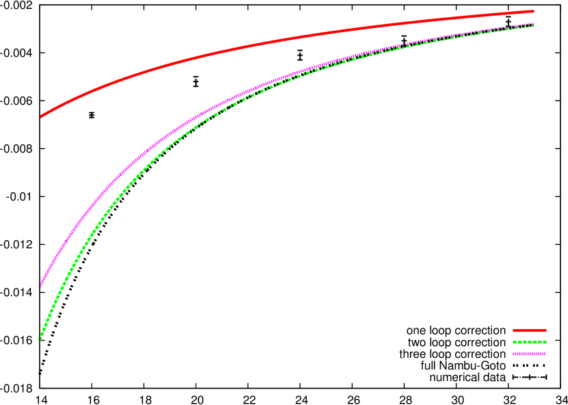
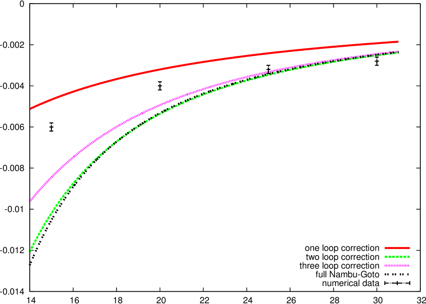
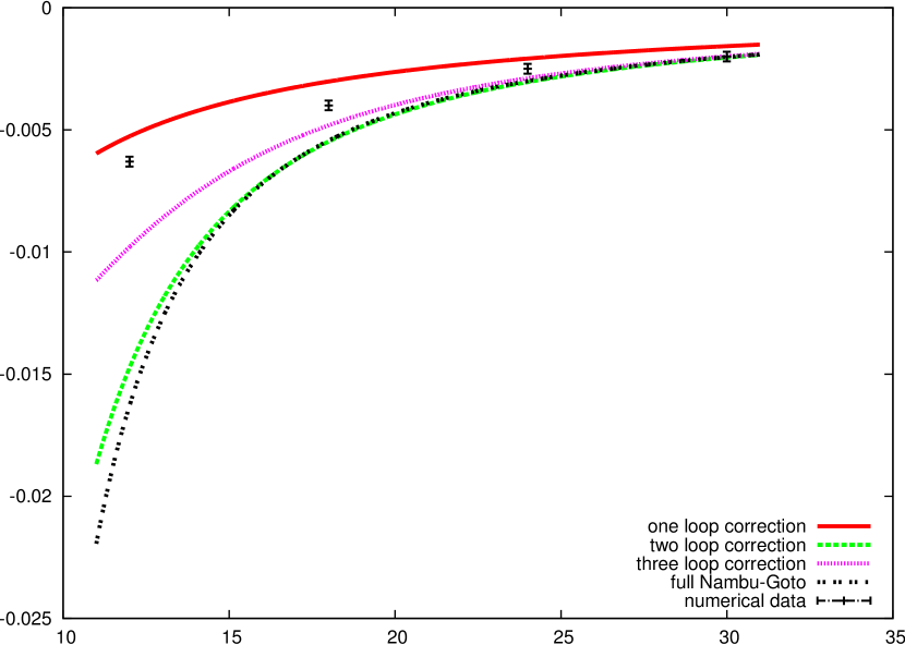
$R_{\mathrm{w}}^{{}^{\prime}}(L,\frac{3}{4}L,1)$	$R_{\mathrm{w}}^{{}^{\prime}}(L,\frac{4}{5}L,1)$
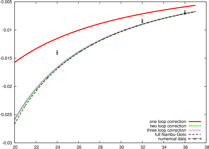
$R_{\mathrm{w}}^{{}^{\prime}}(L,\frac{5}{6}L,1)$	$R_{\mathrm{w}}^{{}^{\prime}}(L,\frac{3}{4}L,3)$

Figure 4: Plot of $R_{\mathrm{w}}^{{}^{\prime}}(L,\frac{L}{u},n)$ for various values of $u$ and $n$ against the quantum string corrections up to three loop and the whole Nambu Goto prediction.

Remarkably enough, the three loop correction turns out to have the opposite sign with respect to the two loop one and thus it goes exactly in the same direction as the numerical data. The statistical errors are too large to allow any reliable test but, as it can be seen in fig. (4) the gap between two and three loop corrections increases as $R$ decreases and in principle, once the boundary corrections will be under control, this particular combination of Wilson loops could become a perfect setting for high precision tests of the universality conjectures. In this framework it is also interesting to notice that this change of sign is somehow peculiar of the three loop correction and is not present in the whole Nambu-Goto correction (which is also reported in fig. (4) for comparison). While a good agreement of the data with the three loop correction is certainly expected due to universality, the whole Nambu-Goto action should instead be excluded: it cannot be the correct effective action, by the arguments reviewed in the Introduction. The data seem indeed to support this statement, even if, as for the three loop case, the statistical errors are too large to allow any reliable statement and a definitive answer will require a precise control of the boundary correction in order to study the corrections in the range $R<20$.

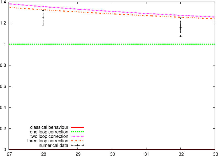
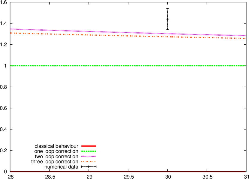
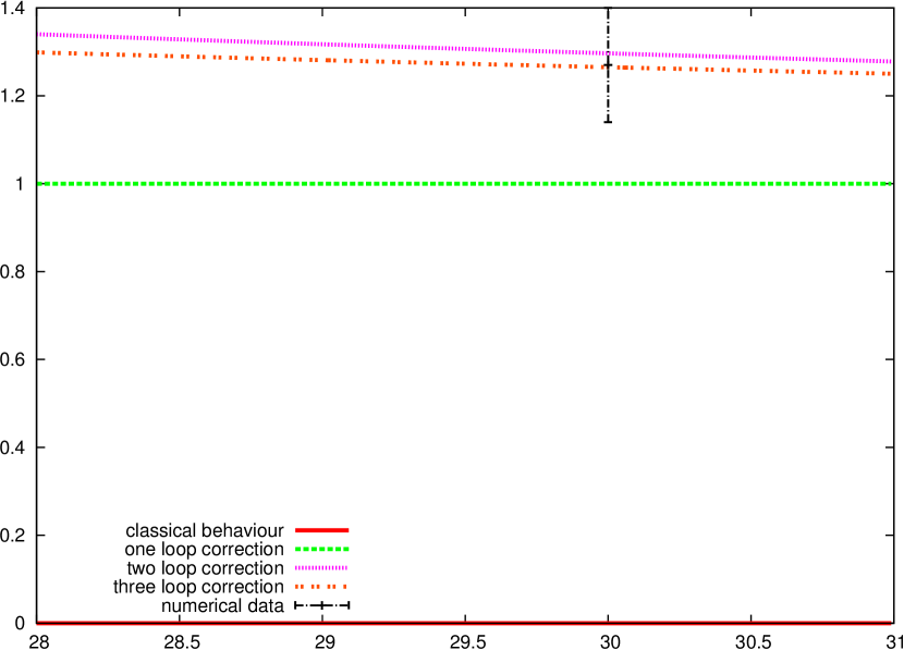
$R_{\mathrm{w}}^{{}^{\prime}}(L,\frac{3}{4}L,1)$	$R_{\mathrm{w}}^{{}^{\prime}}(L,\frac{4}{5}L,1)$
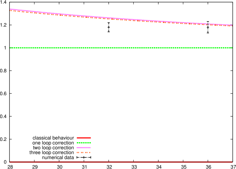
$R_{\mathrm{w}}^{{}^{\prime}}(L,\frac{5}{6}L,1)$	$R_{\mathrm{w}}^{{}^{\prime}}(L,\frac{3}{4}L,3)$

Figure 5: Same as fig.(4, but keeping only the data for $R>20$ which are not affected by boundary conditions (see the main text). To make easier the comparison between the predictions at different orders, we report here the ratio of $R_{\mathrm{w}}^{{}^{\prime}}$ to the one-loop prediction; the error bars are rescaled accordingly.

6 Conclusions

In this paper we have considered the disk partition function for the Nambu-Goto effective string theory corresponding to a rectangular Wilson loop. Our aim was to check the prediction of the NG model including its quantum corrections up to three loops against a numerical simulation tailored to this goal. This purpose, which goes beyond the tests available in the literature, owes its interest to the theorem which states that the corrections up to three loops are universal for all effective string models; a check of the NG model to this order would in fact represent a stringent test of the very idea of an effective string description.

Setting up such a test required progresses both on the theoretical side and on the side of simulations.

On the theoretical side, we have extended to the Wilson loop geometry an operatorial approach based on the first order re-formulation of the NG model that had been already used for the cylinder and torus geometry. The operatorial evaluation makes use of open string analogues of boundary states and leads to an exact expression. This result resums the loop expansion that arises in the physical gauge approach, and can be expanded to the desired loop order. In particular, we have determined the three-loop correction, which had not been obtained in the physical gauge approach.

On the numerical side, we set up the Montecarlo simulation of an observable corresponding to the ratio of two Wilson loops. This observable is devised so as to minimize the effects of boundary terms in the effective action, for which theoretical predictions are not available. Our simulation has been carried out in the 3d Ising gauge model, and has reached a level of precision such that it confirms nicely the validity of the effective string approach up to two loops; this already represents a big improvement with respect to the avaliable literature. The statistical errors are yet too large to test reliably the three loop correction, even though it seems to go in the right direction.

Acknowledgments We thank F. Gliozzi and I. Pesando for useful discussions. We expecially thank L. Ferro and V. Verduci, who participated to the early stages of this work. M.B. thanks the participants to the first week of the ”String Phenomenology 2011” program at NORDITA, and in particular C. Angelantonj, M. Berg, P. Di Vecchia, G. Ferretti, M. Frau, A. Lerda, A. Mariotti, C. Petersson, R. Russo, A. Schellekens, for a stimulating discussion session on subjects related to this work.

Appendix A Notation, conventions and useful formulæ

Here we establish our notations and give some properties of modular functions and Bessel functions that we use in the main text, expecially in section 4.

Dedekind function and Eisenstein series

Dedekind’s $\eta$-function is defined, in terms of the quantity $q=\exp\{2\pi\mathrm{i}\tau\}$, by

$$\eta(\tau)=q^{\frac{1}{24}}\prod_{n=1}^{\infty}\left(1-q^{n}\right)~{}.$$ (62)

One can expand its inverse in $q$-series:

$$[\eta(\tau)]^{-1}=\sum_{k=0}^{\infty}p_{k}\,q^{k-\frac{1}{24}}~{},$$ (63)

where $p_{k}$ denotes the number of partitions of $k$. Other powers of $\eta$ admit a similar Fourier expansion, and we make use of this fact in eq. (46).

Under the generators of modular transformations the Dedekind eta function transforms in the following way:

$$\eta(\tau+1) =\mathrm{e}^{\frac{\mathrm{i}\pi}{12}}\eta(\tau)~{},$$ (64)

$$\eta(-1/\tau) =(\mathrm{e}^{-\mathrm{i}\frac{\pi}{2}}\tau)^{\frac{1}{2}}\eta(\tau)~{}.$$

Eisenstein series can be defined through their Fourier expansion, which takes the form

$$E_{2k}(\tau)=1+\frac{2}{\zeta(1-2k)}\sum_{n=1}^{\infty}\sigma_{2k-1}(n)\,q^{n}~{},$$ (65)

where $\sigma_{2k-1}(n)$ is the sum of the $(2k-1)$-th power of the divisors of $n$:

$$\sigma_{\alpha}(n)=\sum_{d|n}d^{\alpha}~{}.$$ (66)

In particular, we have thus

$$E_{2}(\tau) =1-24\sum_{n=1}^{\infty}\sigma_{1}(n)\,q^{n}~{},$$ (67)

$$E_{4}(\tau) =1+240\sum_{n=1}^{\infty}\sigma_{3}(n)\,q^{n}~{},$$

$$E_{6}(\tau) =1-504\sum_{n=1}^{\infty}\sigma_{5}(n)\,q^{n}~{}.$$

For $k>1$, the Eisenstein series are modular forms of weights $2k$:

$$E_{2k}\left(\frac{A\tau+B}{C\tau+D}\right)=(C\tau+D)^{2k}E_{2k}(\tau)~{},$$ (68)

so that in particular

$$E_{4}(-1/\tau)=\tau^{4}E_{4}(\tau)~{},~{}~{}~{}E_{6}(-1/\tau)=\tau^{6}E_{4}(\tau)~{}.$$ (69)

The series $E_{2}(\tau)$, instead, is almost a modular form of degree 2, since its transformation under the $S$-generator has a non-homogeneus term:

$$E_{2}(-\frac{1}{\tau})=\tau^{2}E_{2}(\tau)-\frac{6}{\pi}\mathrm{i}\tau~{}.$$ (70)

Taking into account these transformation properties, it is not difficult to check that the various expressions given in section 4.2, and in particular eq. (56), are invriant under the exchange $L\leftrightarrow R$, i.e., $u\leftrightarrow 1/u$.

The $E_{2}$ series is related to Dedekind $\eta$-function by

$$\frac{1}{2\pi\mathrm{i}}\partial_{\tau}\log\eta(\tau)=q\partial_{q}\log\eta(\tau)=\frac{1}{24}E_{2}(\tau)~{}.$$ (71)

Further derivatives connect $E_{2}$ to $E_{4}$ and $E_{6}$:

$$q\partial_{q}E_{2} =-\frac{1}{12}(E_{4}-E_{2}^{2})~{},$$ (72)

$$q\partial_{q}E_{4} =-\frac{1}{3}(E_{6}-E_{2}E_{4})~{},$$

$$q\partial_{q}E_{6} =-\frac{1}{2}(E_{4}^{2}-E_{2}E_{6})~{}.$$

Applying these formulæ, we can evaluate the multiple logarithmic derivatives with respect to $Q=\exp(2\pi\mathrm{i}u)$ that appear in eq. (55):

$$\left(Q\frac{d\phantom{Q}}{dQ}\right)\left[\eta(\mathrm{i}u)\right]^{-\alpha} =-\frac{\alpha}{24}\left[\eta(\mathrm{i}u)\right]^{-\alpha}E_{2}(\mathrm{i}u)~{},$$ (73)

$$\left(Q\frac{d\phantom{Q}}{dQ}\right)^{2}\left[\eta(\mathrm{i}u)\right]^{-\alpha} =\frac{\alpha}{(24)^{2}}\left[\eta(\mathrm{i}u)\right]^{-\alpha}\Bigl{(}2E_{4}(\mathrm{i}u)+(\alpha-2)E_{2}^{2}(\mathrm{i}u)\Bigr{)}~{},$$

$$\left(Q\frac{d\phantom{Q}}{dQ}\right)^{3}\left[\eta(\mathrm{i}u)\right]^{-\alpha} =-\frac{\alpha}{(24)^{3}}\left[\eta(\mathrm{i}u)\right]^{-\alpha}\Bigl{(}16E_{6}(\mathrm{i}u)+6(\alpha-4)E_{4}(\mathrm{i}u)E_{2}(\mathrm{i}u)$$

$$+(\alpha^{2}-6\alpha+8)E_{2}^{3}(\mathrm{i}u)\Bigr{)}~{},$$

$$\left(Q\frac{d\phantom{Q}}{dQ}\right)^{4}\left[\eta(\mathrm{i}u)\right]^{-\alpha} =\frac{\alpha}{(24)^{4}}\left[\eta(\mathrm{i}u)\right]^{-\alpha}\Bigl{(}64(\alpha-6)E_{6}(\mathrm{i}u)E_{2}(\mathrm{i}u)+12(\alpha+12)E_{4}^{2}(\mathrm{i}u)$$

$$+12(\alpha^{2}-10\alpha+24)E_{4}(\mathrm{i}u)E_{2}^{2}(\mathrm{i}u)+(\alpha^{3}-12\alpha^{2}+44\alpha-48)E_{2}^{4}(\mathrm{i}u)\Bigr{)}~{}.$$

Asymptotic expansion of Bessel Functions

The asympotic expansion of the modified Bessel functions of the second kind $K_{\alpha}(z)$ for large values of their argument $z$ takes the form

$$K_{\alpha}(z)\sim\sqrt{\frac{\pi}{2z}}\mathrm{e}^{-z}\sum_{m}\frac{1}{m!}\frac{\textstyle\Gamma(\alpha+m+\frac{1}{2})}{\textstyle\Gamma(\alpha-m+\frac{1}{2})}\frac{1}{(2z)^{m}}~{}.$$ (74)

References

- [1] K. G. Wilson, Confinement of Quarks, Phys.Rev. D10 (1974) 2445–2459.
- [2] S. Mandelstam, Vortices and Quark Confinement in Nonabelian Gauge Theories, Phys.Rept. 23 (1976) 245–249.
- [3] H. B. Nielsen and P. Olesen, Vortex Line Models for Dual Strings, Nucl.Phys. B61 (1973) 45–61.
- [4] G. ’t Hooft, A Two-Dimensional Model for Mesons, Nucl.Phys. B75 (1974) 461.
- [5] A. M. Polyakov, String Representations and Hidden Symmetries for Gauge Fields, Phys.Lett. B82 (1979) 247–250.
- [6] A. M. Polyakov, Gauge Fields as Rings of Glue, Nucl.Phys. B164 (1980) 171–188.
- [7] Y. Nambu, Strings, Monopoles and Gauge Fields, Phys.Rev. D10 (1974) 4262.
- [8] Y. Nambu, QCD and the String Model, Phys.Lett. B80 (1979) 372.
- [9] M. Luscher, K. Symanzik, and P. Weisz, Anomalies of the Free Loop Wave Equation in the WKB Approximation, Nucl.Phys. B173 (1980) 365.
- [10] M. Luscher, Symmetry Breaking Aspects of the Roughening Transition in Gauge Theories, Nucl.Phys. B180 (1981) 317.
- [11] Y. Nambu ”in Symmetries and Quark Models, ed. R. Chand, (Gordon and Breach, New York” (1970) .
- [12] T. Goto, Relativistic quantum mechanics of one-dimensional mechanical continuum and subsidiary condition of dual resonance model, Prog.Theor.Phys. 46 (1971) 1560–1569.
- [13] K. Dietz and T. Filk, On the renormalization of string functionals, Phys.Rev. D27 (1983) 2944.
- [14] M. Teper, Large N and confining flux tubes as strings - a view from the lattice, Acta Phys. Polon. B40 (2009) 3249–3320, arXiv:0912.3339 [hep-lat].
- [15] M. Luscher and P. Weisz, String excitation energies in SU(N) gauge theories beyond the free-string approximation, JHEP 07 (2004) 014, arXiv:hep-th/0406205.
- [16] H. B. Meyer, Poincare invariance in effective string theories, JHEP 05 (2006) 066, arXiv:hep-th/0602281.
- [17] O. Aharony and E. Karzbrun, On the effective action of confining strings, JHEP 06 (2009) 012, arXiv:0903.1927 [hep-th].
- [18] O. Aharony and M. Field, On the effective theory of long open strings, JHEP 1101 (2011) 065, arXiv:1008.2636 [hep-th].
- [19] O. Aharony and N. Klinghoffer, Corrections to Nambu-Goto energy levels from the effective string action, JHEP 12 (2010) 058, arXiv:1008.2648 [hep-th].
- [20] M. Caselle, R. Fiore, F. Gliozzi, M. Hasenbusch, K. Pinn, et al., Rough interfaces beyond the Gaussian approximation, Nucl.Phys. B432 (1994) 590–620, arXiv:hep-lat/9407002 [hep-lat].
- [21] M. Caselle, M. Hasenbusch, and M. Panero, The Interface free energy: Comparison of accurate Monte Carlo results for the 3D Ising model with effective interface models, JHEP 0709 (2007) 117, arXiv:0707.0055 [hep-lat].
- [22] M. Caselle, M. Hasenbusch, and M. Panero, High precision Monte Carlo simulations of interfaces in the three-dimensional ising model: A Comparison with the Nambu-Goto effective string model, JHEP 0603 (2006) 084, arXiv:hep-lat/0601023 [hep-lat].
- [23] M. Caselle, M. Hasenbusch, and M. Panero, String effects in the 3-d gauge Ising model, JHEP 0301 (2003) 057, arXiv:hep-lat/0211012 [hep-lat].
- [24] M. Caselle, M. Hasenbusch, and M. Panero, Comparing the Nambu-Goto string with LGT results, JHEP 03 (2005) 026, arXiv:hep-lat/0501027.
- [25] M. Caselle and M. Zago, A new approach to the study of effective string corrections in LGTs, Eur.Phys.J. C71 (2011) 1658, arXiv:1012.1254 [hep-lat]. * Temporary entry *.
- [26] M. Billo and M. Caselle, Polyakov loop correlators from D0-brane interactions in bosonic string theory, JHEP 0507 (2005) 038, arXiv:hep-th/0505201 [hep-th].
- [27] M. Billo, M. Caselle, and L. Ferro, The Partition function of interfaces from the Nambu-Goto effective string theory, JHEP 0602 (2006) 070, arXiv:hep-th/0601191 [hep-th].
- [28] M. Billo, M. Caselle, and L. Ferro, Universal behaviour of interfaces in 2d and dimensional reduction of Nambu-Goto strings, Nucl.Phys. B795 (2008) 623–634, arXiv:0708.3302 [hep-th].
- [29] M. B. Green, J. Schwarz, and E. Witten, Superstring Theory. Vol. 1: Introduction,.
- [30] J. Polchinski, String theory. Vol. 1: An introduction to the bosonic string,.
- [31] P. Olesen, Strings and QCD, Phys.Lett. B160 (1985) 144.
- [32] A. M. Polyakov, Quantum Geometry of Bosonic Strings, Phys.Lett. B103 (1981) 207–210.
- [33] J. Polchinski and A. Strominger, Effective string theory, Phys.Rev.Lett. 67 (1991) 1681–1684.
- [34] J. M. Maldacena, The large N limit of superconformal field theories and supergravity, Adv.Theor.Math.Phys. 2 (1998) 231–252, arXiv:hep-th/9711200 [hep-th].
- [35] S. S. Gubser, I. R. Klebanov, and A. M. Polyakov, Gauge theory correlators from non-critical string theory, Phys. Lett. B428 (1998) 105–114, arXiv:hep-th/9802109.
- [36] E. Witten, Anti-de Sitter space and holography, Adv. Theor. Math. Phys. 2 (1998) 253–291, arXiv:hep-th/9802150.
- [37] A. M. Polyakov, The wall of the cave, Int.J.Mod.Phys. A14 (1999) 645–658, arXiv:hep-th/9809057 [hep-th].
- [38] M. Caselle, R. Fiore, F. Gliozzi, M. Hasenbusch, and P. Provero, String effects in the Wilson loop: A High precision numerical test, Nucl.Phys. B486 (1997) 245–260, arXiv:hep-lat/9609041 [hep-lat].
- [39] B. Durhuus, H. B. Nielsen, P. Olesen, and J. Petersen, Dual Models As Saddle Point Approximations To Polyakov’S Quantized String, Nucl.Phys. B196 (1982) 498.
- [40] B. Durhuus, P. Olesen, and J. Petersen, Polyakov’S Quantized String With Boundary Terms, Nucl.Phys. B198 (1982) 157.
- [41] B. Durhuus, P. Olesen, and J. Petersen, Polyakov’S Quantized String With Boundary Terms. 2, Nucl.Phys. B201 (1982) 176.
- [42] P. Di Vecchia, B. Durhuus, P. Olesen, and J. Petersen, Fermionic Strings With Boundary Terms, Nucl.Phys. B207 (1982) 77.
- [43] O. Alvarez, Theory of Strings with Boundaries: Fluctuations, Topology, and Quantum Geometry, Nucl.Phys. B216 (1983) 125.
- [44] M. Billo’, M. Caselle, V. Verduci, and M. Zago, New results on the effective string corrections to the inter-quark potential, PoS LATTICE2010 (2010) 273, arXiv:1012.3935 [hep-lat]. * Temporary entry *.
- [45] M. Caselle, M. Hasenbusch, and M. Panero, Short distance behaviour of the effective string, JHEP 05 (2004) 032, arXiv:hep-lat/0403004.
- [46] S. Necco and R. Sommer, The N(f) = 0 heavy quark potential from short to intermediate distances, Nucl. Phys. B622 (2002) 328–346, arXiv:hep-lat/0108008.
- [47] B. B. Brandt, Probing boundary-corrections to Nambu-Goto open string energy levels in 3d SU(2) gauge theory, JHEP 02 (2011) 040, arXiv:1010.3625 [hep-lat].
- [48] Y. Imamura, H. Isono, and Y. Matsuo, Boundary states in open string channel and CFT near corner, Prog.Theor.Phys. 115 (2006) 979–1002, arXiv:hep-th/0512098 [hep-th].
- [49] C. G. Callan, Jr., C. Lovelace, C. R. Nappi and S. A. Yost, Loop Corrections to Superstring Equations of Motion, Nucl.Phys.B 308 (1988) 221
- [50] P. Di Vecchia and A. Liccardo, D-branes in string theory. 1., NATO Adv.Study Inst.Ser.C.Math.Phys.Sci. 556 (2000) 1–59, arXiv:hep-th/9912161 [hep-th].
- [51] B. Durhuus, P. Olesen and J. L. Petersen, Nucl. Phys. B 232 (1984) 291.
- [52] P. Orland, Evolution of fixed end strings and the off-shell disk amplitude, Nucl.Phys. B605 (2001) 64–80, arXiv:hep-th/0101173 [hep-th].