Model independent analysis of top quark forward-backward asymmetry at the Tevatron up to $\mathcal{O}(\alpha_{s}^{2}/\Lambda^{2})$

Abstract

We present the complete calculations of the forward-backward asymmetry ($A_{\rm FB}$) and the total cross section of top quark pair production induced by dimension-six four quark operators at the Tevatron up to $\mathcal{O}(\alpha_{s}^{2}/\Lambda^{2})$. Our results show that next-to-leading order (NLO) QCD corrections can change $A_{\rm FB}$ and the total cross section by about 10%. Moreover, NLO QCD corrections reduce the dependence of $A_{\rm FB}$ and total cross section on the renormalization and factorization scales significantly. We also evaluate the total cross section and the charge asymmetry ($A_{\rm C}$) induced by these operators at the Large Hadron Collider (LHC) up to $\mathcal{O}(\alpha_{s}^{2}/\Lambda^{2})$, for the parameter space allowed by the Tevatron data. We find that the value of $A_{\rm C}$ induced by these operators is much larger than SM prediction, and LHC has potential to discover these NP effects when the measurement precision increases.

I INTRODUCTION

The top quark is the heaviest particle discovered so far, with a mass close to the electroweak symmetry breaking scale. Thus it is a wonderful probe for the electroweak breaking mechanism and new physics (NP) beyond the standard model (SM) through its productions and decays at colliders. The forward-backward asymmetry ($A_{\rm FB}$) of the top quark pair production is one of the interesting observables at hadron colliders. Within the SM, $A_{\rm FB}$ is absent at the tree level in QCD due to charge symmetry, and occurs at next-to-leading order (NLO) $\mathcal{O}(\alpha_{s}^{3})$ in QCD with the prediction $A_{\rm FB}\sim 6\%$ in the $t\bar{t}$ rest frame Kuhn and Rodrigo (1998, 1999); Bowen et al. (2006); Almeida et al. (2008); Antunano et al. (2008); Ahrens et al. (2011). In the last few years, DØ and CDF Collaborations measured $A_{\rm FB}$ at the Tevatron Abazov et al. (2008); Aaltonen et al. (2008, 2011); collaboration (2011). Recently, the CDF Collaborations annouced that, for the invariant mass of the top quark pair $m_{t\bar{t}}\geq 450$ GeV, the measured asymmetry, $A_{\rm FB}=0.475\pm 0.114$Aaltonen et al. (2011), differs by 3.4$\sigma$ from the SM predictions $A_{\rm FB}=0.088\pm 0.013$, which has aroused many discussions of explaining this deviation in NP model, including new gauge bosons, axigluons and so onDjouadi et al. (2010); Jung et al. (2010a); Cheung et al. (2009); Frampton et al. (2010); Shu et al. (2010); Arhrib et al. (2010); Ferrario and Rodrigo (2010); Dorsner et al. (2010); Jung et al. (2010b); Cao et al. (2010a); Barger et al. (2010); Cao et al. (2010b); Xiao et al. (2010); Martynov and Smirnov (2010); Chivukula et al. (2010); Bauer et al. (2010); Chen et al. (2011a); Jung et al. (2011a); Burdman et al. (2011); Jung et al. (2010c); Choudhury et al. (2010); Cheung and Yuan (2011); Cao et al. (2011); Berger et al. (2011); Barger et al. (2011); Bhattacherjee et al. (2011); Blum et al. (2011a); Patel and Sharma (2011); Isidori and Kamenik (2011); Zerwekh (2011); Barreto et al. (2011); Foot (2011); Ligeti et al. (2011); Gresham et al. (2011); Jung et al. (2011d); Buckley et al. (2011); Shu et al. (2011); Aguilar-Saavedra and Perez-Victoria (2011b); Chen et al. (2011b); Degrande et al. (2011a); Jung et al. (2011c, b); Babu et al. (2011); Djouadi et al. (2011); Barcelo et al. (2011a); Krohn et al. (2011); Aguilar-Saavedra and Perez-Victoria (2011c); Cui et al. (2011); Hektor et al. (2011); Gabrielli and Raidal (2011); Duraisamy et al. (2011); Aguilar-Saavedra and Perez-Victoria (2011a); Barcelo et al. (2011b); Tavares and Schmaltz (2011); Vecchi (2011); Blum et al. (2011b); Degrande et al. (2011b); Aguilar-Saavedra and Perez-Victoria (2011d).
Since we do not know which type of NP will be responsible for this deviation, it is interesting to study the $A_{\rm FB}$ in a model independent way, using an effective Lagrangian. In general, NP scale relevant to $A_{\rm FB}$ is large enough so that the heavy fields have been integrated out at the low energy scale. At the Tevatron, the subprocess $q\bar{q}\to t\bar{t}$ dominates over top quark pair production, so only contributions from dimension-six four quark operators to the $t\bar{t}$ production are considered. Similar approach had been adopted for the dijet production to constrain the composite scale of light quarks Eichten et al. (1983, 1984); Chiappetta and Perrottet (1991); Eichten and Lane (1996); Gao et al. (2011). The relevant effective Lagrangian can be written as

$$\mathcal{L}_{NP}=\frac{1}{\Lambda^{2}}\sum_{A,B}\left[C^{1}_{AB}\left(\bar{q}_{A}\gamma_{\mu}q_{A}\right)\left(\bar{t}_{B}\gamma^{\mu}t_{B}\right)+C^{8}_{AB}\left(\bar{q}_{A}T^{a}\gamma_{\mu}q_{A}\right)\left(\bar{t}_{B}T^{a}\gamma^{\mu}t_{B}\right)\right],$$ (1)

where $\{A,B\}=\{L,R\}$ with $q=(u,d)^{T},(c,s)^{T}$. Up to $\mathcal{O}(\alpha_{s}/\Lambda^{2})$, the NP contributions to the total cross section and the $A_{\rm FB}$ are clear in the vector-axial basis Degrande et al. (2011b); Blum et al. (2011a); Kamenik et al. (2011), as compared with the chirality basis. Only the axial-axial current combination contributions to the $A_{\rm FB}$, and the vector-vector operator contributes to the total cross section. However, this is no longer true up to $\mathcal{O}(\alpha_{s}^{2}/\Lambda^{2})$. The chirality basis is the preferred one when studying the chiral structure of NP effects much above the Electroweak scale, so we choose to work in the chirality basis. The contributions to $A_{\rm FB}$ at leading order (LO) from such operators has been explored in Refs. Jung et al. (2010b, 2011a, d, c); Degrande et al. (2011b); Aguilar-Saavedra and Perez-Victoria (2011d). It is shown that the $A_{\rm FB}$ observed at the Tevatron can be explained by above operators for suitable parameters. As we know, the LO cross section at hardron colliders suffers from large uncertainties due to the arbitrary choice of the renormalization scale and factorization scale, thus it is important to include NLO corrections to improve theoretical predictions. Besides, at the NLO level, virtual corrections, real gluon emission and massless (anti)quark emission can lead to a sizeable difference between the differential top and anti-top production process Kuhn and Rodrigo (1998, 1999), which will contribute to $A_{\rm FB}$.
In this paper, we present the complete NLO QCD calculations of $A_{\rm FB}$ and the total cross section of top quark pair production at the Tevatron induced by above operators, and we also study the top quark pair production at the Large Hadron Collider (LHC) induced by these operators at the NLO QCD level. Last year, LHC reported their first observation of top quark pair production, and will soon become a major top quark factory. At the LHC, the top quark pairs can be produced through quark antiquark annihilation $q\bar{q}\to t\bar{t}$ and gluon fusion $gg\to t\bar{t}$. Since gluon fusion channel dominates at the LHC, it is difficult to probe these four quark effective operators from early LHC results. However, it is still possible to detect these effects from above effective operators on the Charge Asymmetry($A_{\rm C}$) at the LHC, in the parameter space allowed by the Tevatron data, when the measurement precision increases.
The arrangement of this paper is as follows. In Sec. II we show the LO results. In Sec. III, we present the details of the NLO calculations, including the virtual and real corrections to the top quark pair production. Section IV contains the numerical results, and Section V is a brief summary.

II LO results

Throughout our calculation, we adopt the same conventions as in Ref. Zhu et al. (2011) (see Sec. III A), and present the helicity amplitudes for $q\bar{q}\to t\bar{t}$ in the Four-Dimensional Helicity (FDH) regularization scheme Bern et al. (2002). The $t\bar{t}$ production amplitudes, including NP contributions, can be written as

$$\mathcal{M}_{t\bar{t}}=\alpha_{s}f_{\rm LO}^{\rm SM}+\frac{1}{\Lambda^{2}}f_{\rm LO}^{\rm NP}+\alpha_{s}^{2}f_{\rm NLO}^{\rm SM}+\frac{\alpha_{s}}{\Lambda^{2}}f_{\rm NLO}^{\rm NP}+\cdots,$$ (2)

and thus the partonic cross section, up to $\mathcal{O}(\alpha_{s}^{2}/\Lambda^{2})$, can be written as

$$\hat{\sigma}_{t\bar{t}} = \alpha_{s}^{2}f_{\rm LO}^{\rm SM}f^{\rm SM^{\ast}}_{\rm LO}+2\frac{\alpha_{s}}{\Lambda^{2}}\mathcal{R}e\left(f_{\rm LO}^{\rm SM}f^{\rm NP^{\ast}}_{\rm LO}\right)$$ (3)

$$+2\alpha_{s}^{3}\mathcal{R}e\left(f_{\rm LO}^{\rm SM}f^{\rm SM^{\ast}}_{\rm NLO}\right)+2\frac{\alpha_{s}^{2}}{\Lambda^{2}}\left[\mathcal{R}e\left(f_{\rm LO}^{\rm NP}f^{\rm SM^{\ast}}_{\rm NLO}\right)+\mathcal{R}e\left(f_{\rm LO}^{\rm SM}f^{\rm NP^{\ast}}_{\rm NLO}\right)\right].$$

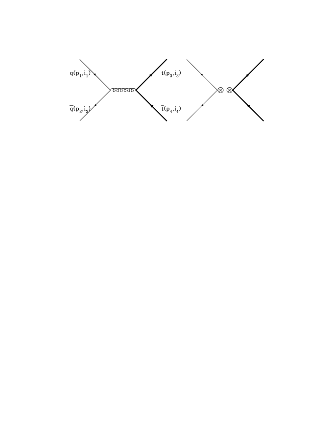
Figure 1: LO Feynman diagrams for $q\bar{q}\rightarrow t\bar{t}$ induced by SM QCD and NP interactions.

The LO Feynman diagrams for the subprocess $q(p_{1})\bar{q}(p_{2})\rightarrow t(p_{3})\bar{t}(p_{4})$ induced by the SM QCD and the NP interactions are shown in Fig. 1, and their ($+-++$) helicity amplitudes are

$$\mathcal{M}_{\textrm{LO}}^{\textrm{SM}}(+-++) = \frac{i8\pi\alpha_{s}m_{t}}{s}\left(\mathcal{M}_{1}+\mathcal{M}_{2}\right)\mathcal{C}_{8},$$ (4)

$$\mathcal{M}_{\textrm{LO}}^{\textrm{NP}}(+-++) = \frac{i2m_{t}}{\Lambda^{2}}\left[\left(\mathcal{M}_{1}C_{\rm RR}^{1}+\mathcal{M}_{2}C_{\rm RL}^{1}\right)\mathcal{C}_{1}+\left(\mathcal{M}_{1}C_{\rm RR}^{8}+\mathcal{M}_{2}C_{\rm RL}^{8}\right)\mathcal{C}_{8}\right],$$ (5)

where the SM QCD and NP contributions are denoted by superscipts SM and NP, and Mandelstam variables $s$, $t$ and $u$ are defined as follows:

$$s=(p_{1}+p_{2})^{2},~{}~{}~{}t=(p_{1}-p_{3})^{2},~{}~{}~{}u=(p_{1}-p_{4})^{2}.$$ (6)

We define the following abbreviations for the color structures and matrix elements,

$$\mathcal{M}_{1}=\frac{\langle\eta_{4}1\rangle\langle\eta_{3}|\textbf{3}|2]}{\langle 3^{\flat}\eta_{3}\rangle\langle\eta_{4}4^{\flat}\rangle}, \mathcal{M}_{2}=\frac{\langle\eta_{3}1\rangle\langle\eta_{4}|\textbf{4}|2]}{\langle 3^{\flat}\eta_{3}\rangle\langle\eta_{4}4^{\flat}\rangle},$$

$$\mathcal{M}_{3}=\frac{\langle\eta_{4}2\rangle\langle\eta_{3}|\textbf{3}|1]}{\langle 3^{\flat}\eta_{3}\rangle\langle\eta_{4}4^{\flat}\rangle}, \mathcal{M}_{4}=\frac{\langle\eta_{3}2\rangle\langle\eta_{4}|\textbf{4}|1]}{\langle 3^{\flat}\eta_{3}\rangle\langle\eta_{4}4^{\flat}\rangle},$$

$$\mathcal{C}_{1}=\delta_{i_{2}i_{1}}\delta_{i_{3}i_{4}}, \mathcal{C}_{8}=T^{a}_{i_{2}i_{1}}T^{a}_{i_{3}i_{4}},$$ (7)

where $i_{1...4}$ are the color indices of the external quarks and the boldface momenta denotes massive vectors. We use the modified spinor helicity method suited for massive particles Kleiss and Stirling (1985) in our calculations, and a recent application of this method can be found in the Ref Badger et al. (2011). The ($-+++$) amplitudes are given by

$$\mathcal{M}_{\rm{LO}}^{\rm{SM}}(-+++) = \frac{i8\pi\alpha_{s}m_{t}}{s}\left(\mathcal{M}_{3}+\mathcal{M}_{4}\right)\mathcal{C}_{8},$$ (8)

$$\mathcal{M}_{\rm{LO}}^{\rm{NP}}(-+++) = \frac{i2m_{t}}{\Lambda^{2}}\left[\left(\mathcal{M}_{3}C_{\rm LR}^{1}+\mathcal{M}_{4}C_{\rm LL}^{1}\right)\mathcal{C}_{1}+\left(\mathcal{M}_{3}C_{\rm LR}^{8}+\mathcal{M}_{4}C_{\rm LL}^{8}\right)\mathcal{C}_{8}\right].$$ (9)

The amplitudes with other helicity configurations can be obtained from ($+-++$) and ($-+++$) by exchanging light-like momenta $p^{\flat}$ and $\eta$ Zhu et al. (2011); Badger et al. (2011). At the LO, there is only vector current coupling $\bar{\psi}\gamma^{\mu}\psi$ at the massive quark vertex. At the NLO, however, magnetic-momentum coupling $\bar{\psi}(i\sigma^{\mu\nu}(p_{3}+p_{4})_{\mu})\psi/(2m_{t})$ is induced from loop diagrams. For completeness we list the matrix elements for magnetic-moment interaction,

$$\mathcal{M}_{1}^{(m)}=\frac{m_{t}^{2}\langle\eta_{3}1\rangle\langle\eta_{4}1\rangle[21]}{\langle 3^{\flat}\eta_{3}\rangle\langle\eta_{4}4^{\flat}\rangle}, \mathcal{M}_{2}^{(m)}=\frac{\langle 12\rangle\langle\eta_{3}|\textbf{3}|2]\langle\eta_{4}|\textbf{4}|2]}{\langle 3^{\flat}\eta_{3}\rangle\langle\eta_{4}4^{\flat}\rangle},$$

$$\mathcal{M}_{3}^{(m)}=\frac{m_{t}^{2}\langle\eta_{3}2\rangle\langle\eta_{4}2\rangle[21]}{\langle 3^{\flat}\eta_{3}\rangle\langle\eta_{4}4^{\flat}\rangle}, \mathcal{M}_{4}^{(m)}=\frac{\langle 12\rangle\langle\eta_{3}|\textbf{3}|1]\langle\eta_{4}|\textbf{4}|1]}{\langle 3^{\flat}\eta_{3}\rangle\langle\eta_{4}4^{\flat}\rangle}.$$ (10)

After phase space integration, the $\mathcal{O}(\alpha_{s}/\Lambda^{2})$ partonic differential cross section is

$$\frac{d\hat{\sigma}^{\textrm{NP}}_{\rm{LO}}}{dcos\theta} = \frac{\beta}{18}\frac{\alpha_{s}}{\Lambda^{2}}\left[\frac{1}{4}(1+\rho+\beta^{2}cos^{2}\theta)(C^{8}_{\rm LR}+C^{8}_{\rm RR})+\frac{1}{2}\beta\cos\theta(C^{8}_{\rm RR}-C^{8}_{\rm LR})\right],$$ (11)

where $\rho=4m_{t}^{2}/s$, $\beta=\sqrt{1-\rho^{2}}$, and $\theta$ is the polar angle between the incoming quark and the outgoing top quark in the $t\bar{t}$ rest frame. The color and spin indices are averaged(summed) over initial(final) states. In Eq. (11) the term linear in $\cos\theta$ could generate $A_{\rm FB}$ proportional to $\rm\left(C^{8}_{RR}-C^{8}_{LR}\right)$ and the rest terms contribute to the total cross section proportional to $\rm\left(C^{8}_{RR}+C^{8}_{LR}\right)$. These relations will be changed at the NLO level.
The LO total cross section at the hadron collider is obtained by convoluting the partonic level cross section with the Parton Distribution Function (PDF) $f_{i/A}$ for the initial hadron A:

$$\sigma_{\rm{LO}}=\sum_{a,b}\int_{\tau}^{1}dx_{a}\int_{\tau/x_{a}}^{1}dx_{b}f_{a/A}(x_{a},\mu_{f})f_{b/B}(x_{b},\mu_{f})\hat{\sigma}_{\rm{LO}},$$ (12)

where $\tau=4m_{t}^{2}/s$. The sum is over all possible initial partons.

III NLO QCD corrections

The NLO corrections to the top pair production consist of the virtual corrections, generated by loop diagrams of colored particles, and the real corrections with the radiation of a real gluon or a massless (anti)quark. We carried out all the calculations in the ’t Hooft-Feynman gauge and used the FDH scheme to regularize all the divergences. Moveover, for the real corrections, we used the dipole substraction method with massive partons Catani et al. (2002) to separate the infrared (IR) divergences, which is convenient for the case of massive Feynman diagrams and provides better numerical accuracy.

III.1 Virtual corrections

The virtual corrections for the top quark pair production include the box diagrams, triangle diagrams, and self-energy diagrams in SM QCD and NP as shown in Fig. 2 and Fig. 3. We have calculated the one-loop helicity amplitudes for the SM process, and find complete agreement with those in the Ref. Zhu et al. (2011); Korner and Merebashvili (2002). Here we only list the NP contributions.

Figure 2: One-loop virtual Feynman diagrams for $q\bar{q}\rightarrow t\bar{t}$ induced by SM QCD interactions.

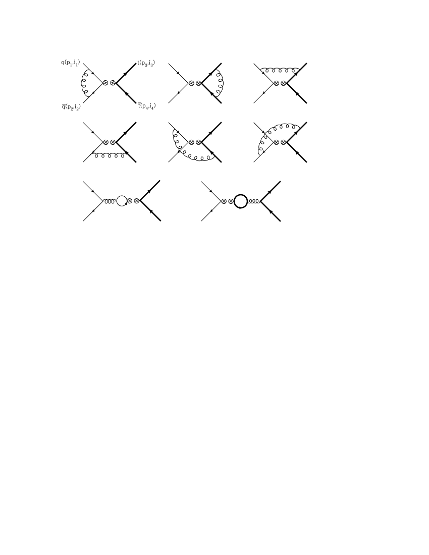
Figure 3: One-loop virtual Feynman diagrams for $q\bar{q}\rightarrow t\bar{t}$ induced by NP interactions.

All the ultraviolet (UV) divergences in the loop diagrams are canceled by counterterms for the wave functions of the external fields ($\delta Z_{q},\delta Z_{t}$), and the Wilsion coefficients $\delta Z_{C^{i}_{AB}}$. For the external fields, we fix all the renormalization constants using on-shell subtraction, and, therefore, they also have IR singularities

$$\delta Z_{q} = -\frac{\alpha_{s}}{4\pi}C_{\varepsilon}C_{F}\left(\frac{1}{\varepsilon_{UV}}-\frac{1}{\varepsilon_{IR}}\right),$$ (13)

$$\delta Z_{t} = -\frac{\alpha_{s}}{4\pi}C_{\varepsilon}C_{F}\left(\frac{1}{\varepsilon_{UV}}+\frac{2}{\varepsilon_{IR}}+5-3\ln\frac{m_{t}^{2}}{\mu_{r}^{2}}\right),$$ (14)

where $C_{\varepsilon}=(4\pi)^{\varepsilon}\frac{1}{\Gamma(1-\varepsilon)}$ , $C_{F}=4/3$ and $\mu_{r}$ is the renormalization scale. For contourterms of the Wilsion coefficients $\delta Z_{C^{i}_{AB}}$, we adopted the $\rm\overline{MS}$ scheme

$$\delta Z_{C^{i}_{AB}}=\frac{\alpha_{s}}{4\pi}C_{\varepsilon}C_{F}\frac{1}{\varepsilon_{UV}}\left(\begin{array}[]{cccccccc}0&\frac{9}{8}&0&0&0&0&0&0\\ \frac{1}{4}&\frac{n_{f}-5}{16}&0&\frac{1}{16}&0&\frac{n_{f}}{16}&0&0\\ 0&0&0&-\frac{9}{8}&0&0&0&0\\ 0&\frac{1}{16}&-\frac{1}{4}&\frac{n_{f}-20}{16}&0&0&0&\frac{n_{f}}{16}\\ 0&0&0&0&0&-\frac{9}{8}&0&0\\ 0&\frac{n_{f}}{16}&0&0&-\frac{1}{4}&\frac{n_{f}-20}{16}&0&\frac{1}{16}\\ 0&0&0&0&0&0&0&\frac{9}{8}\\ 0&0&0&\frac{n_{f}}{16}&0&\frac{1}{16}&\frac{1}{4}&\frac{n_{f}-5}{16}\end{array}\right),$$ (23)

where $n_{f}=5$ is the number of massless quarks appearing in the closed loop diagram, and the order of the Wilsion coefficients is

$$\left(C_{\rm LL}^{1},C_{\rm LL}^{8},C_{\rm LR}^{1},C_{\rm LR}^{8},C_{\rm RL}^{1},C_{\rm RL}^{8},C_{\rm RR}^{1},C_{\rm RR}^{8}\right).$$ (24)

We have considered mixing effects of different color and chiral operators, and the evolution equations of the Wilson coefficients are given in the Appendix B. The renormalized virtual amplitudes can be written as

$$\mathcal{M}^{V}=\mathcal{M}^{\textrm{unren}}+\mathcal{M}^{\textrm{con}}.$$ (25)

Here $\mathcal{M}^{\rm unren}$ contains the self-energy and vertex corrections, and $\mathcal{M}^{\textrm{con}}$ are the corresponding counterterms. The renormalized amplitude $\mathcal{M}^{V}$ is UV finite, but still contains IR divergences, which are given by

$$\mathcal{M}_{\rm{SM}}^{\rm{IR}} = \frac{\alpha_{s}}{2\pi}C_{\varepsilon}C_{F}\left[f_{\text{os}}^{\rm{IR}}\mathcal{C}_{1}\mathcal{M}_{8}^{\rm{SM}}+f_{\text{oo}}^{\rm{IR}}\mathcal{C}_{8}\mathcal{M}_{8}^{\rm{SM}}\right],$$ (26)

$$\mathcal{M}_{\rm{NP}}^{\rm{IR}} = \frac{\alpha_{s}}{2\pi}C_{\varepsilon}C_{F}\left[f_{\text{ss}}^{\rm{IR}}\mathcal{C}_{1}\mathcal{M}_{1}^{\rm{NP}}+f_{\text{so}}^{\rm{IR}}\mathcal{C}_{8}\mathcal{M}_{1}^{\rm{NP}}+f_{\text{os}}^{\rm{IR}}\mathcal{C}_{1}\mathcal{M}_{8}^{\rm{NP}}+f_{\text{oo}}^{\rm{IR}}\mathcal{C}_{8}\mathcal{M}_{8}^{\rm{NP}}\right],$$ (27)

where we define the IR divergence coefficients $f_{\text{ss}}^{\text{IR}}$, $f_{\text{so}}^{\text{IR}}$, $f_{\text{os}}^{\text{IR}}$ and $f_{\text{oo}}^{\text{IR}}$ for different color configurations, ”s” for singlet and ”o” for octect,

$$f_{\text{ss}}^{\text{IR}} = -\frac{1}{\varepsilon_{\rm{IR}}^{2}}+\frac{1}{\varepsilon_{\rm{IR}}}\left[\frac{1}{2}\left(\beta+\frac{1}{\beta}\right)\ln\left(\frac{\beta+1}{\beta-1}\right)+\ln\left(\frac{-s}{\mu_{r}^{2}}\right)-\frac{5}{2}\right],$$ (28)

$$f_{\text{so}}^{\text{IR}} = \frac{3}{2}\ln\left(\frac{t_{1}}{u_{1}}\right)\frac{1}{\varepsilon_{\rm{IR}}},$$ (29)

$$f_{\text{os}}^{\text{IR}} = \frac{1}{3}\ln\left(\frac{t_{1}}{u_{1}}\right)\frac{1}{\varepsilon_{\rm{IR}}},$$ (30)

$$f_{\text{oo}}^{\text{IR}} = -\frac{1}{\varepsilon_{\rm{IR}}^{2}}+\frac{1}{\varepsilon_{\rm{IR}}}\Bigg{[}-\frac{1}{16}\left(\beta+\frac{1}{\beta}\right)\ln\left(\frac{\beta+1}{\beta-1}\right)-\frac{9}{8}\ln\left(\frac{m_{t}^{2}}{\mu_{r}^{2}}\right)-\frac{1}{8}\ln\left(\frac{-s}{\mu_{r}^{2}}\right)$$ (31)

$$+\frac{7}{4}\ln\left(\frac{t_{1}}{\mu_{r}^{2}}\right)+\frac{1}{2}\ln\left(\frac{u_{1}}{\mu_{r}^{2}}\right)-\frac{5}{2}\Bigg{]},$$

where $t_{1}=m_{t}^{2}-t$, $u_{1}=m_{t}^{2}-u$ and $\mathcal{M}_{1}^{\rm{NP}}$, $\mathcal{M}_{8}^{\rm{NP}}$ and $\mathcal{M}_{8}^{\rm{SM}}$ are defined as follows,

$$\mathcal{M}^{\rm{SM}}_{\rm LO} = \mathcal{M}_{8}^{\rm{SM}}\mathcal{C}_{8},$$ (32)

$$\mathcal{M}^{\rm{NP}}_{\rm LO} = \mathcal{M}_{1}^{\rm{NP}}\mathcal{C}_{1}+\mathcal{M}_{8}^{\rm{NP}}\mathcal{C}_{8}.$$ (33)

Since we only consider high order corrections up to $\mathcal{O}(\alpha_{s}^{2}/\Lambda^{2})$, the IR divergences of the virtual corrections can be written as

$$2\mathcal{R}e\left[\mathcal{M}_{\rm{SM}}^{\rm{IR}}\mathcal{M}_{\rm{NP}}^{\rm{LO}^{\ast}}\right]+2\mathcal{R}e\left[\mathcal{M}_{\rm{NP}}^{\rm{IR}}\mathcal{M}_{\rm{SM}}^{\rm{LO}^{\ast}}\right]$$ (34)

$$= \frac{\alpha_{s}}{\pi}C_{\varepsilon}C_{F}\left[\left(9f_{\text{os}}^{\rm{IR}}+2f_{\text{so}}^{\rm{IR}}\right)\mathcal{R}e\left(\mathcal{M}_{1}^{\rm{NP}^{\ast}}\mathcal{M}_{8}^{\rm{SM}}\right)+4f_{\text{oo}}^{\rm{IR}}\mathcal{R}e\left(\mathcal{M}_{8}^{\rm{NP}^{\ast}}\mathcal{M}_{8}^{\rm{SM}}\right)\right].$$

The finite terms in $\mathcal{M}^{V}_{\rm NP}$ are given in the Appendix A.

III.2 Real corrections

At the NLO level the real corrections consist of the radiations of an additional gluon or massless (anti)quark in the final states, including the subprocess

$$q\bar{q}\to t\bar{t}g,~{}~{}~{}gq(\bar{q})\to t\bar{t}q(\bar{q})$$ (35)

as shown in Fig.4 and Fig.5.

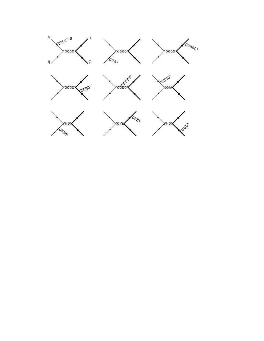
Figure 4: Feynman diagrams for the real gluon emission contributions induced by SM QCD and NP interactions.

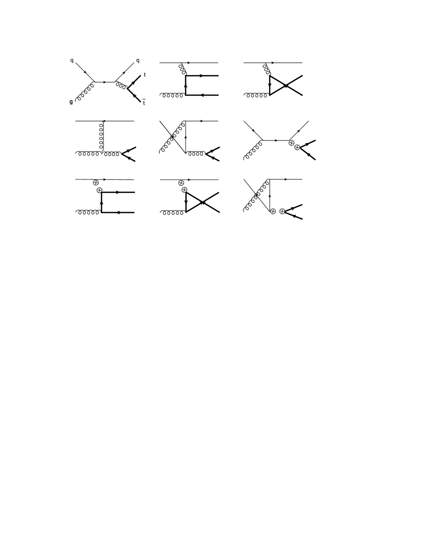
Figure 5: Feynman diagrams for the massless quark emission contributions induced by SM QCD and NP interactions.

Before performing the numerical calculations, we need to extract the IR divergences in the real corrections. In the dipole formalism this is done by subtracting some dipole terms from the real corrections to cancel the singularities and large logarithms exactly, and then the real corrections become integrable in four dimensions. On the other hand, these dipole subtraction terms are analytically integrable in $n$ dimensions over one-parton subspaces, which give $\varepsilon$ poles that represent the soft and collinear divergences. Then we can add them to the virtual corrections to cancel the $\varepsilon$ poles, and ensure the virtual corrections are also integrable in four dimensions. This whole procedure can be illustrated by the formula Catani et al. (2002):

$$\hat{\sigma}^{\rm NLO}=\int_{m+1}\left[\left(d\hat{\sigma}^{\rm{R}}\right)_{\varepsilon=0}-\left(d\hat{\sigma}^{\rm{A}}\right)_{\varepsilon=0}\right]+\int_{m}\left[d\hat{\sigma}^{\rm{V}}+\int_{1}d\hat{\sigma}^{\rm{A}}\right]_{\varepsilon=0},$$ (36)

where $m$ is the number of final state particles at the LO, and $d\hat{\sigma}^{\rm{A}}$ is a sum of the dipole terms. Besides, at hadron colliders, we have to include the well-known collinear subtraction counterterms in order to cancel the collinear divergences arising from the splitting processes of the initial state massless partons. Here we use the $\overline{\rm MS}$ scheme and the corresponding NLO PDFs.

For the process with two initial state hadrons, the dipole terms can be classified into four groups, the final-state emitter and final-state spectator type,

$$\mathcal{D}_{ij,k}(p_{1},...,p_{m+1})=$$

$$\qquad-{1\over(p_{i}+p_{j})^{2}-m_{ij}^{2}}{\ {}_{m}}\langle...,\widetilde{ij},...,\widetilde{k},...|\frac{\textbf{T}_{k}\cdot\textbf{T}_{ij}}{\textbf{T}_{ij}^{2}}{\textbf{V}_{ij,k}}|...,\widetilde{ij},...,\widetilde{k},...\rangle_{m},$$ (37)

the final-state emitter and initial-state spectator type,

$$\mathcal{D}_{ij}^{a}(p_{1},...,p_{m+1};p_{a},...)=$$

$$\qquad-{1\over(p_{i}+p_{j})^{2}-m_{ij}^{2}}\frac{1}{x_{ij,a}}{\ {}_{m,a}}\langle...,\widetilde{ij},...;\widetilde{a},...|\frac{\textbf{T}_{a}\cdot\textbf{T}_{ij}}{\textbf{T}_{ij}^{2}}{\textbf{V}_{ij}^{a}}|...,\widetilde{ij},...;\widetilde{a},...\rangle_{m,a},$$ (38)

the initial-state emitter and final-state spectator type,

$$\mathcal{D}_{j}^{ai}(p_{1},...,p_{m+1};p_{a},...)=$$

$$\qquad-{1\over 2p_{a}p_{i}}\frac{1}{x_{ij,a}}{\ {}_{m,\widetilde{ai}}}\langle...,\widetilde{j},...;\widetilde{ai},...|\frac{\textbf{T}_{j}\cdot\textbf{T}_{ai}}{\textbf{T}_{ai}^{2}}{\textbf{V}_{j}^{ai}}|...,\widetilde{j},...;\widetilde{ai},...\rangle_{m,\widetilde{ai}},$$ (39)

and the initial-state emitter and initial-state spectator type,

$$\mathcal{D}^{ai,b}(p_{1},...,p_{m+1};p_{a},p_{b})=$$

$$\qquad-{1\over 2p_{a}p_{i}}\frac{1}{x_{i,ab}}{\ {}_{m,\widetilde{ai}}}\langle...;\widetilde{ai},b|\frac{\textbf{T}_{b}\cdot\textbf{T}_{ai}}{\textbf{T}_{ai}^{2}}{\textbf{V}^{ai,b}}|...;\widetilde{ai},b\rangle_{m,\widetilde{ai}},$$ (40)

where $a,b$ and $i,j,...$ are the initial and final state partons, and T and V are the color charge operators and dipole functions acting on the LO amplitudes, respectively. The explicit expressions for $x_{i,ab}$, $x_{ij,a}$ and V can be found in Ref. Catani et al. (2002). The integrated dipole functions together with the collinear counterterms can be written in the following factorized form

$$\sim \int d\Phi^{(m)}(p_{a},p_{b})\ _{m,ab}\langle...;p_{a},p_{b}|\textbf{I}_{m+a+b}(\varepsilon)|...;p_{a},p_{b}\rangle_{m,ab}$$ (41)

$$+\sum_{a^{\prime}}\int_{0}^{1}dx\int d\Phi^{(m)}(xp_{a},p_{b})_{m,a^{\prime}b}\langle...;xp_{a},p_{b}|\textbf{P}_{m+b}^{a,a^{\prime}}(x)+\textbf{K}_{m+b}^{a,a^{\prime}}(x)|...;xp_{a},p_{b}\rangle_{m,a^{\prime}b}$$

$$\qquad\qquad\qquad+(a\leftrightarrow b),$$

where $x$ is the momentum fraction of the splitting parton, $d\Phi^{(m)}$ contains all the factors apart from the squared amplitudes, I, P, and K are insertion operators defined in Catani et al. (2002). For simplicity, in all the above formulas we do not show the jet functions that define the observables and are included in our numerical calculations.

The operators P and K provide finite contributions to the NLO corrections, and only the operator I contains the IR divergences

$$\textbf{I}|_{\rm{IR}} = -\frac{\alpha_{s}}{2\pi}{(4\pi)^{\varepsilon}\over\Gamma(1-\varepsilon)}\bigg{\{}\sum_{j}\sum_{k\neq j}\textbf{T}_{j}\cdot\textbf{T}_{k}\bigg{[}\left(\frac{\mu_{r}^{2}}{s_{jk}}\right)^{\varepsilon}\mathcal{V}(s_{jk},m_{j},m_{k};\varepsilon_{IR})+{1\over\textbf{T}_{j}^{2}}\Gamma_{j}(m_{j},\varepsilon_{IR})\bigg{]}$$ (42)

$$+\sum_{j}\textbf{T}_{j}\cdot\textbf{T}_{a}\bigg{[}2\left(\frac{\mu_{r}^{2}}{s_{ja}}\right)^{\varepsilon}\mathcal{V}(s_{ja},m_{j},0;\varepsilon_{IR})+{1\over\textbf{T}_{j}^{2}}\Gamma_{j}(m_{j},\varepsilon_{IR})+{1\over\textbf{T}_{a}^{2}}\frac{\gamma_{a}}{\varepsilon_{IR}}\bigg{]}$$

$$+\textbf{T}_{a}\cdot\textbf{T}_{b}\bigg{[}\left(\frac{\mu_{r}^{2}}{s_{ab}}\right)^{\varepsilon}\left(\frac{1}{\varepsilon_{IR}^{2}}+{1\over\textbf{T}_{a}^{2}}\frac{\gamma_{a}}{\varepsilon_{IR}}\right)\bigg{]}+(a\leftrightarrow b)\bigg{\}},$$

with

$$\mathcal{V}(s_{jk},m_{j},m_{k};\varepsilon_{IR}) = {1\over v_{jk}}\left(\frac{Q_{jk}^{2}}{s_{jk}}\right)^{\varepsilon}\times\left(1-{1\over 2}\rho_{j}^{-2\varepsilon}-{1\over 2}\rho_{k}^{-2\varepsilon}\right){1\over\varepsilon_{IR}^{2}},$$

$$\Gamma_{j}(0,\varepsilon_{IR}) = \frac{\gamma_{j}}{\varepsilon_{IR}},\quad\Gamma_{j}(m_{j}\neq 0,\varepsilon_{IR})=\frac{C_{F}}{\varepsilon_{IR}},$$ (43)

where $C_{F}=4/3$, $\gamma_{q}=2$, and $\gamma_{g}=11/2-n_{f}/3$. And $s_{jk}$, $Q_{jk}^{2}$, $v_{jk}$, and $\rho_{n}$ are kinematic variables defined as follows

$$s_{jk} = 2p_{j}p_{k},\quad Q_{jk}^{2}=s_{jk}+m_{j}^{2}+m_{k}^{2},\quad v_{jk}=\sqrt{1-\frac{m_{j}^{2}m_{k}^{2}}{(p_{j}p_{k})^{2}}},$$

$$\rho_{n} = \sqrt{\frac{1-v_{jk}+2m_{n}^{2}/(Q_{jk}^{2}-m_{j}^{2}-m_{k}^{2})}{1+v_{jk}+2m_{n}^{2}/(Q_{jk}^{2}-m_{j}^{2}-m_{k}^{2})}}\quad(n=j,k).$$ (44)

When inserting Eq. (42) into the LO amplitudes for the $q\bar{q}$ and $qg$ subprocesses as shown in Eq. (41), we can see that the IR divergences, including the $1/\epsilon_{\rm IR}$ terms, can be written as combinations of the LO color correlated squared amplitudes and all the IR divergences from the virtual corrections in Eq. (34) are canceled exactly, as we expected.

IV Numerical Results

In the Lagrangian $\mathcal{L}_{NP}$, there are totally nine free parameter $C_{\rm LL}^{1}$, $C_{\rm LR}^{1}$, $C_{\rm RL}^{1}$, $C_{\rm RR}^{1}$, $C_{\rm LL}^{8}$, $C_{\rm LR}^{8}$, $C_{\rm RL}^{8}$, $C_{\rm RR}^{8}$ and $\Lambda$. If we include left-handed top quark $t_{L}$ in the $\mathcal{L}_{NP}$, it is suitable to work in $SU(2)_{L}$ doublet of the third-generation quarks $(t_{\rm L},b_{\rm L})^{T}$. However, the Wilson coefficients $C_{\rm LL}^{1}$, $C_{\rm LL}^{8}$, $C_{\rm RL}^{1}$ and $C_{\rm RL}^{8}$ are highly constrained by the LEP data for the ratio of $b\bar{b}$ to hadron production Nakamura et al. (2010):

$$B_{b}=0.121629\pm 0.00066,$$ (45)

which agrees well with the SM prediction. Thus, for simplicity we choose $C_{\rm LL}^{1}=C_{\rm LL}^{8}=C_{\rm RL}^{1}=C_{\rm RL}^{8}=0$ Jung et al. (2010b). Up to $\mathcal{O}(\alpha_{s}^{2}/\Lambda^{2})$, contributions from color singlet operators due to mixing effects are much less than contributions from color octet operators, so we only consider color octet interactions. As a result, in the numerical calculations there are only three free NP parameters in the Lagrangian, i.e. $C_{\rm LR}^{8}$, $C_{\rm RR}^{8}$ and $\Lambda$.
Top quark mass is taken to be $m_{t}=172.5~{}{\rm GeV}$. We choose CTEQ6L and CTEQ6M PDF sets Pumplin et al. (2002) and the associated $\alpha_{s}$ functions for LO and NLO calculation, respectively. Both the renormalization and factorization scales are fixed to the top quark mass unless specified. We have used the modified MadDipole Frederix et al. (2008) package for the real corrections.

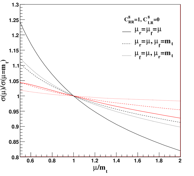
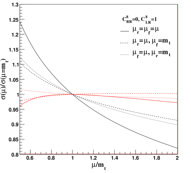
Figure 6: Scale dependence of the total cross section at the Tevetron, the black and the red lines represent LO and NLO results, respectively.

IV.1 Scale dependence

In Fig. 6 we show the scale dependence of the LO and NLO total cross section at the Tevatron for three cases: (1) the renormalization scale dependence $\mu_{r}=\mu,\ \mu_{f}=m_{t}$, (2) the factorization scale dependence $\mu_{r}=m_{t},\ \mu_{f}=\mu$, and (3) total scale dependence $\mu_{r}=\mu_{f}=\mu$. It can be seen that the NLO corrections reduce the scale dependence significantly for all three cases, which makes the theoretical predictions more reliable.

IV.2 Tevatron constraints

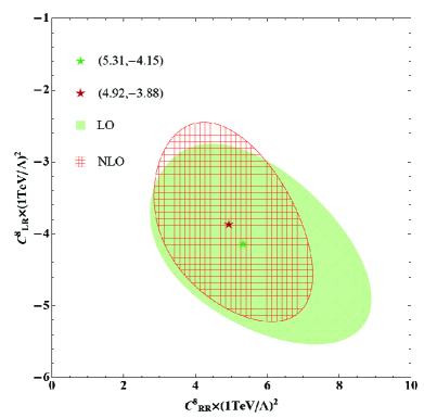
Figure 7: Values of $C_{RR}^{8}$ and $C_{LR}^{8}$ allowed by the Tavetron data at 1$\sigma$ CL: $\sigma_{t\bar{t}}$=(7.50 $\pm$ 0.48)pb and $A_{\textrm{FB}}\left(m_{t\bar{t}}>450~{}\textrm{GeV}\right)$=0.475$\pm$0.114. The green star $\rm(5.31,-4.15)$ and red star $\rm(4.92,-3.88)$ represent the BFPs at LO and NLO level, respectively.

$A_{\textrm{FB}}$ of top quark pair productions is defined as

$$A_{\textrm{FB}} = \frac{\sigma_{\textrm{F}}-\sigma_{\textrm{B}}}{\sigma_{\textrm{F}}+\sigma_{\textrm{B}}}$$

$$= A_{\textrm{FB}}^{\textrm{NP}}\times R+A_{\textrm{FB}}^{\textrm{SM}}\times(1-R)$$

where

$$A_{\textrm{FB}}^{\textrm{NP}} = (\sigma_{\textrm{F}}^{\textrm{NP}}-\sigma_{\textrm{B}}^{\textrm{NP}})/(\sigma_{\textrm{F}}^{\textrm{NP}}+\sigma_{\textrm{B}}^{\textrm{NP}}),$$

$$A_{\textrm{FB}}^{\textrm{SM}} = (\sigma_{\textrm{F}}^{\textrm{SM}}-\sigma_{\textrm{B}}^{\textrm{SM}})/(\sigma_{\textrm{F}}^{\textrm{SM}}+\sigma_{\textrm{B}}^{\textrm{SM}}),$$

$$R = \sigma_{\textrm{tot}}^{\textrm{NP}}/(\sigma_{\textrm{tot}}^{\textrm{SM}}+\sigma_{\textrm{tot}}^{\textrm{NP}})$$ (46)

are the asymmetries induced by NP and SM, and $R$ is the fraction of NP contribution to the total cross section. $\sigma_{\textrm{F}}$ and $\sigma_{\rm B}$ denote the total cross sections in the forward(F) and backward(B) rapidity regions, respectively. Up to order $O(\alpha_{s}^{2}/\Lambda^{2})$, total cross sections induced by NP can be written as

$$\sigma^{\textrm{NP}}_{\textrm{LO}} = \left[(0.428^{+0.103}_{-0.076})C_{\rm RR}^{8}+(0.428^{+0.101}_{-0.075})C_{\rm LR}^{8}\right]\left(\frac{1\text{TeV}}{\Lambda}\right)^{2}~{}\textrm{pb},$$ (47)

$$\sigma^{\textrm{NP}}_{\textrm{NLO}} = \left[(0.442^{+0.018}_{-0.032})C_{\rm RR}^{8}+(0.435^{+0.022}_{-0.022})C_{\rm LR}^{8}\right]\left(\frac{1\text{TeV}}{\Lambda}\right)^{2}~{}\textrm{pb},$$ (48)

and the difference of the cross section in the forward and backward rapidity regions can be written as

$$\left[\sigma_{\textrm{F}}^{\textrm{NP}}-\sigma_{\textrm{B}}^{\textrm{NP}}\right]^{m_{t\bar{t}}>450~{}\textrm{GeV}}_{\textrm{LO}} = \left[(0.118^{+0.031}_{-0.023})C_{\rm RR}^{8}-(0.118^{+0.031}_{-0.023})C_{\rm LR}^{8}\right]\left(\frac{1\text{TeV}}{\Lambda}\right)^{2}~{}\textrm{pb},$$ (49)

$$\left[\sigma_{\textrm{F}}^{\textrm{NP}}-\sigma_{\textrm{B}}^{\textrm{NP}}\right]^{m_{t\bar{t}}>450~{}\textrm{GeV}}_{\textrm{NLO}} = \left[(0.149^{+0.003}_{-0.009})C_{\rm RR}^{8}-(0.103^{+0.008}_{-0.025})C_{\rm LR}^{8}\right]\left(\frac{1\text{TeV}}{\Lambda}\right)^{2}~{}\textrm{pb},$$ (50)

where the errors are obtained by varying the scale between $\mu_{r}=\mu_{f}=m_{t}/2$ and $\mu_{r}=\mu_{f}=2m_{t}$. From the expressions Eqs.(47 – 50) we can see that NLO corrections reduce the dependence of $\sigma_{\textrm{F}}^{\textrm{NP}}-\sigma_{\textrm{B}}^{\textrm{NP}}$ and $\sigma^{\textrm{NP}}$ on the renormalization and factorization scales significantly.
In Fig. 7, we show the allowed region in the $(C_{\rm RR}^{8},C_{\rm LR}^{8})$ plane that is consistent with the Tevatron data Aaltonen et al. (2011):

$$\sigma_{t\bar{t}}^{\rm EX} = (7.50\pm 0.48)\textrm{pb},$$

$$\rm{A_{FB}^{EX}} = 0.475\pm 0.114,~{}~{}~{}~{}{\rm for}~{}m_{t\bar{t}}>450~{}\rm{GeV}.$$ (51)

We use Monte Carlo programm MCFM Campbell and Ellis (1999) to get the cross section of the gluon fusion channel $gg\to t\bar{t}$ at the NLO QCD level. As for the process of $q\bar{q}\to t\bar{t}$, we have checked our value with the results given by MCFM at QCD NLO level, which are well consistent in the range of Monte Carlo integration error. Combining the contributions of these two channels we have the total cross section of $t\bar{t}$ production

$$\sigma_{t\bar{t}}^{\textrm{SM}} = 7.00^{+0.36}_{-0.76}~{}\textrm{pb},$$ (52)

where we have considered scale uncertainty in the calculations. For consistency we have used the SM predicted values of $A_{\rm FB}\left(m_{t\bar{t}}\geq 450\rm{GeV}\right)=0.088$ at NLO QCD level, although next-to-next-to-leading logarithmic (NNLL) SM QCD results are available Ahrens et al. (2011). In Fig. 7, green and red regions correspond to NP LO and NLO results at 1$\sigma$ confidence level(CL), where we have considered theoretical and experimental uncertainty in the total cross section and only consider experimental uncertainty in the $A_{\rm FB}$ calculation. It can be seen that NLO corrections obviously change the allowed region of $C_{\textrm{RR}}^{8}$ and $C_{\textrm{RR}}^{1}$. The green star $\rm(5.31,-4.15)$ and red star $\rm(4.92,-3.88)$ represent the best-fit point(BFP) at LO and NLO level, respectively, from which we can see higher order corrections reduce the BFP by about 7%. The $t\bar{t}$ total cross sections induced by NP at the NLO BFP $\rm(4.92,-3.88)$ are

$$\sigma^{\rm{NP}}_{t\bar{t},\rm{LO}} = 0.445~{}\rm{pb},$$

$$\sigma^{\rm{NP}}_{t\bar{t},\rm{NLO}} = 0.497~{}\rm{pb},$$ (53)

where the K factor is about 1.12. $A_{\rm FB}$ containing NP contributions at the NLO BFP are shown together in Table 1. The NLO QCD corrections to $A_{\rm FB}$ can reach about 10%, and the theoretical predictions containing NP NLO effects are consistent with experimental results at 2$\sigma$ CL.

	SM NLO QCD + NP LO	SM NLO QCD + NP NLO
$A_{\rm FB}^{p\bar{p}}$	0.175	0.189 ($\sim$ 0.7 $\sigma$)
$A_{\rm FB}^{t\bar{t}}$	0.252	0.275 ($\sim$ 1.6 $\sigma$)
$A_{\rm FB}^{t\bar{t}}\left(m_{t\bar{t}}<450~{}{\rm GeV}\right)$	0.132	0.136 ($\sim$ 1.6 $\sigma$)
$A_{\rm FB}^{t\bar{t}}\left(m_{t\bar{t}}>450~{}{\rm GeV}\right)$	0.452	0.475 ($\sim$ 0 $\sigma$)
$A_{\rm FB}^{t\bar{t}}\left(|\Delta y|<1\right)$	0.170	0.161 ($\sim$ 0.9 $\sigma$)
$A_{\rm FB}^{t\bar{t}}\left(|\Delta y|>1\right)$	0.719	0.681 ($\sim$ 0.3 $\sigma$)

Table 1: $A_{\rm FB}$ with $\rm C_{RR}^{8}(1TeV/\Lambda)^{2}=4.92$ and $\rm C_{LR}^{8}(1TeV/\Lambda)^{2}=-3.88$ at the Tevtron, where $A_{\rm FB}^{p\bar{p}}$ and $A_{\rm FB}^{t\bar{t}}$ are the $A_{\rm FB}$ in the lab frame and the $t\bar{t}$ rest frame, respectively, and $\Delta y=y_{t}-y_{\bar{t}}$ is the difference of rapidities of the top and antitop quarks. Here we list the CL when containing NP effects at NLO level.

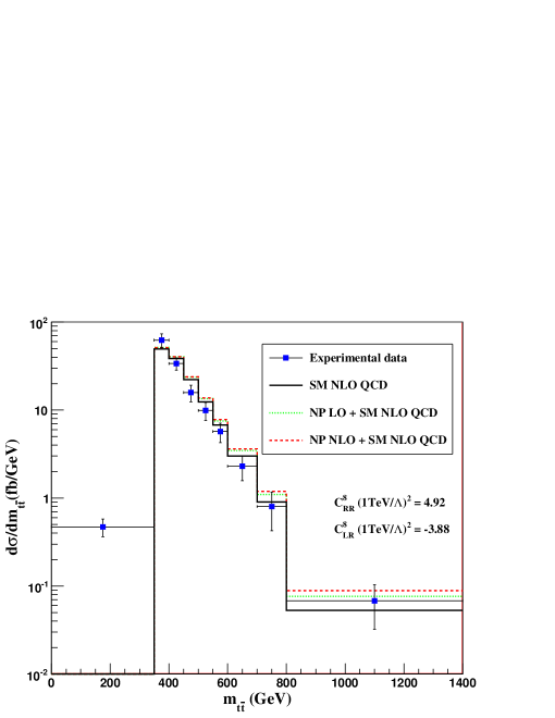
Figure 8: Differential cross sections $d\sigma/dm_{t\bar{t}}$ as a function of $m_{t\bar{t}}$ at the NLO BFP $\rm(4.92,-3.88)$. Here ”Experimental data” is $d\sigma/dm_{t\bar{t}}$ measured with 2.7 $fb^{-1}$ of integrated luminosity at the Tevatron Aaltonen et al. (2009). ”SM NLO QCD” represents the results in the SM QCD at NLO level. ”NP LO + SM NLO QCD” and ”NP NLO + SM NLO QCD” stand for the predictions including NP effects up to $\mathcal{O}(\alpha_{s}/\Lambda^{2})$ and $\mathcal{O}(\alpha_{s}^{2}/\Lambda^{2})$, respectively.

In Fig. 8, we show differential cross section $d\sigma/dm_{t\bar{t}}$ when we consider NP effects at the NLO BFP, from which we can see that higher order corrections do not change the distribution very much.

IV.3 LHC predictions

The process of top quark pair production has been measured at the LHC, and the cross section Cristinziani (2011); Tosi and Collaboration (2011) is

$$\sigma_{t\bar{t}}^{\rm ATLAS}({\rm\sqrt{S}=7~{}TeV})=180\pm 18{\rm pb},$$

$$\sigma_{t\bar{t}}^{\rm CMS}({\rm\sqrt{S}=7~{}TeV})=158\pm 19{\rm pb},$$ (54)

which is consistent with the SM predictions. The NP contributions at the NLO BFP $\rm(4.92,-3.88)$ is about 3 pb, which is much smaller than the experimental uncertainty. Thus, it is difficult to measure the NP effects only through the cross section measurements. In Fig. 9, we show differential cross section $d\sigma/dm_{t\bar{t}}$ at the LHC when we consider NP effects at the NLO BFP $\rm(4.92,-3.88)$, from which we can see that NP contributions almost do not change the distribution.

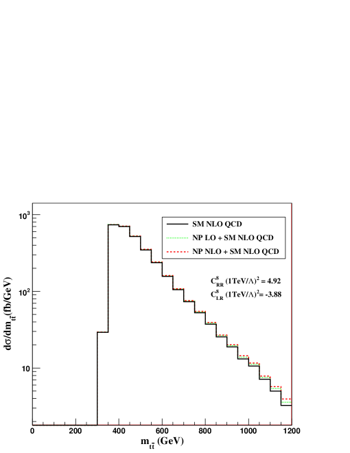
Figure 9: Differential cross sections $d\sigma/dm_{t\bar{t}}$ as a function of $m_{t\bar{t}}$ at the LHC with $\sqrt{S}=7~{}{\rm TeV}$.

Since the LHC is a proton-proton collider, which is forward-backward symmetric, the $A_{\rm FB}$ defined at Tevatron can not be directly applied to the proton-proton collider experiments at the LHC. The $A_{\rm C}$ used by CMS The CMS Collaboration (2011) can be written as

$$A_{\rm C}=\frac{\sigma(|\eta_{t}|-|\eta_{\bar{t}}|>0)-\sigma(|\eta_{t}|-|\eta_{\bar{t}}|<0)}{\sigma(|\eta_{t}|-|\eta_{\bar{t}}|>0)+\sigma(|\eta_{t}|-|\eta_{\bar{t}}|<0)},$$ (55)

where $\eta_{t}$ and $\eta_{\bar{t}}$ are pseudo rapidities of top and antitop quark, respectively. Its value is measured to be

$$A_{\rm C}=-0.016\pm 0.030({\rm stat.})^{+0.010}_{-0.019}({\rm syst.})$$ (56)

which is consistent with the SM predictions: $A_{\rm C}=0.013(11)$ The CMS Collaboration (2011); Ferrario and Rodrigo (2010, 2008). The $A_{\rm C}$ induced by NP interactions at the NP NLO BFP $\rm(4.92,-3.88)$ is 0.063, which is about 5 times larger than SM predictions, and also consistent with the CMS data at about 2$\sigma$ CL.

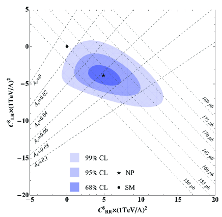
Figure 10: Results of a combined fit to $\sigma_{t\bar{t}}$ and the value of $A_{\rm FB}$ allowing for NP at different CLs. The blue contours from dark to light indicate the experimentally favored region of 68%, 95% and 99% CL in the ($C_{RR}^{8},C_{LR}^{8}$) plane. The black doted and dashed lines respectively represent the value of $t\bar{t}$ cross section and the $A_{\rm C}$ at the LHC with $\sqrt{S}=7$ TeV. The black dot and black star represent the SM point and the NP NLO BFP.

In Fig. 10, we show the results of a combined fit to the $t\bar{t}$ data in the presence of NP at different CLs. The blue contours from dark to light indicate the experimentally preferred region of 68%, 95% and 99% CL in the ($C_{RR}^{8},C_{LR}^{8}$) plane. The black dot represent the SM point $(0,0)$, and the black star represent the NP NLO BFP $\rm(4.92,-3.88)$. The black doted and dashed lines respectively represent the value of $t\bar{t}$ cross section and the $A_{\rm C}$ at the LHC with $\sqrt{S}=7$ TeV. From the location of the blue area, one finds that $A_{\rm C}$ predicted by NP is obviously much larger than SM predictions, and LHC has potential to find this difference when the measurement precision increases.

V Conclusions

In conclusion, we have investigated $A_{\rm FB}$ and total cross section of top quark pair production induced by dimension-six four quark operators at the Tevatron up to $\mathcal{O}(\alpha_{s}^{2}/\Lambda^{2})$. Our results show that, NLO QCD corrections can change $A_{\rm FB}$ and the total cross section by about 10%. Moreover, NLO QCD corrections reduce the dependence of $A_{\rm FB}$ and the total cross sections on the renormalization and factorization scales significantly, which lead to increased confidence on the theoretical predictions. We also evaluate total cross section and $A_{\rm C}$ induced by these operators at the LHC up to $\mathcal{O}(\alpha_{s}^{2}/\Lambda^{2})$, for the parameter space allowed by the Tevatron data. We find that the value of $A_{\rm C}$ induced by these operators is much larger than SM predictions, and LHC has potential to discover these NP effects when the measurement precision increases.

Appendix A FINITE TERMS IN VIRTUAL CORRECTIONS

In this appendix, we collect explicit expressions of finite terms in virtual corrections. Analytical continuation for the Mandelstam variables are defined as

$$s \to s+i\varepsilon,$$

$$u \to u+i\varepsilon,$$

$$t \to t+i\varepsilon.$$ (57)

For simplicity, we introduce the following abbreviations.

$$c_{t}=\frac{m_{t}^{2}-t}{t},~{}~{}c_{u}=\frac{m_{t}^{2}-u}{u},$$ (58)

$$y_{1}(t) = \ln\frac{t_{1}}{\mu_{r}^{2}}+\frac{t_{1}}{2t}-1,$$

$$y_{2}(t) = \ln\frac{m_{t}^{2}}{\mu_{r}^{2}}+\frac{t_{1}}{t}-1,$$

$$y_{3}(t) = \ln\frac{t_{1}}{\mu_{r}^{2}}-\left(\frac{t_{1}}{t}+1\right),$$

$$y_{4}(t) = \ln\frac{m_{t}^{2}}{\mu_{r}^{2}}-2\left(\frac{t_{1}}{t}+2\right),$$ (59)

$$f_{1}(t) = \frac{3}{8t}\left(\frac{2}{c^{2}_{t}}+\frac{2}{c_{t}}+\ln\frac{t_{1}}{m_{t}^{2}}\right),$$

$$f_{2}(t) = \frac{3}{4}\left(1+\frac{1}{c_{t}}\right)\left(1-c_{t}\ln\frac{t_{1}}{m_{t}{}^{2}}\right),$$

$$f_{3}(t) = -\frac{1}{2}y_{1}{}^{2}(t)+\frac{1}{4}y_{2}{}^{2}(t)-\frac{1}{8}c^{2}_{t}-\frac{1}{2c_{t}}-\frac{\pi^{2}}{12}-\frac{5}{4}+\text{Li}_{2}\left(\frac{-t}{t_{1}}\right),$$

$$f_{4}(t) = -\frac{1}{2}y_{3}{}^{2}(t)+\frac{1}{4}y_{4}{}^{2}(t)-\frac{1}{2}c^{2}_{t}-3c_{t}-\frac{1}{c_{t}}-\frac{\pi^{2}}{12}-\frac{3}{2}+\text{Li}_{2}\left(\frac{-t}{t_{1}}\right),$$

$$f_{5}(t,u) = \frac{3}{2}f_{3}(t)-\frac{3}{2}f_{4}(u),$$ (60)

$$h_{1}(s) = \frac{1}{32}\left(\beta+\frac{1}{\beta}\right)\ln\left(\frac{\beta+1}{\beta-1}\right)\left(2\text{ln$\beta$}-3+\ln\frac{m_{t}^{2}}{\mu_{r}^{2}}+\ln\left(\frac{-s}{\mu_{r}^{2}}\right)\right),$$

$$h_{2}(s) = \frac{1}{16}\left(\beta+\frac{1}{\beta}\right)\left(\text{Li}_{2}\left(\frac{\beta-1}{2\beta}\right)-\text{Li}_{2}\left(\frac{\beta+1}{2\beta}\right)\right),$$

$$h_{3}(s) = -\frac{\beta^{3}}{16}\ln\left(\frac{\beta+1}{\beta-1}\right)+\frac{\beta^{2}}{8}+\frac{3\beta}{16}\ln\left(\frac{\beta+1}{\beta-1}\right)+\frac{1}{16}\ln^{2}\left(\frac{-s}{\mu_{r}^{2}}\right),$$

$$-\frac{21}{16}\ln\frac{m_{t}^{2}}{\mu_{r}^{2}}-\frac{3-2n_{f}}{16}\ln\left(\frac{-s}{\mu_{r}^{2}}\right)-\frac{5n_{f}-61}{24},$$

$$h_{4}(s) = -\frac{\beta^{3}}{16}\ln\left(\frac{\beta+1}{\beta-1}\right)+\frac{\beta^{2}}{8}+\frac{5\beta}{32}\ln\left(\frac{\beta+1}{\beta-1}\right)+\frac{1}{8}\ln\frac{m_{t}^{2}}{\mu_{r}^{2}},$$

$$-\frac{1}{3}+\frac{1}{32\beta}\ln\left(\frac{\beta+1}{\beta-1}\right),$$

$$h_{5}(s) = \frac{1}{16s\beta}\ln\left(\frac{\beta+1}{\beta-1}\right),$$

$$h_{6}(s) = n_{f}\left(\frac{1}{8}\ln\left(\frac{-s}{\mu_{r}^{2}}\right)-\frac{5}{24}\right),$$

$$h_{7}(s) = -\frac{1}{2}\ln^{2}\left(\frac{-s}{\mu_{r}^{2}}\right)+\frac{3}{2}\ln\left(\frac{-s}{\mu_{r}^{2}}\right)-2\ln\frac{m_{t}^{2}}{\mu_{r}^{2}}-\frac{1}{2},$$

$$h_{8}(s) = \frac{1}{4}\left(\beta-\frac{1}{\beta}\right)\ln\left(\frac{\beta+1}{\beta-1}\right),$$

$$h_{9}(s) = -8h_{1}(s)-8h_{2}(s)+h_{7}(s),$$ (61)

$$g_{1}\left(s,f_{3}(t),f_{4}(u)\right) = \frac{7}{4}f_{3}(t)+\frac{1}{2}f_{4}(u)+h_{1}(s)+h_{2}(s)+h_{3}(s),$$

$$g_{2}(s,t) = \frac{7}{6}f_{2}(t)+h_{4}(s),$$

$$g_{3}(s,u) = \frac{1}{3}f_{2}(u)+h_{4}(s),$$

$$g_{4}(s,t) = -\frac{7}{6}f_{1}(t)-h_{5}(s),$$

$$g_{5}(s,u) = -\frac{1}{3}f_{1}(u)-h_{5}(s).$$ (62)

First we list the amplitude for helicity $(+-++)$,

$$i\mathcal{M}_{\rm virt}^{\rm NP,fin}(+-++)=\frac{i\alpha_{s}m}{\pi\Lambda^{2}}C_{F}\big{[}\mathcal{M}_{\rm ss}(+-++)\mathcal{C}_{1}+\mathcal{M}_{\rm so}(+-++)\mathcal{C}_{8}$$

$$+\mathcal{M}_{\rm os}(+-++)\mathcal{C}_{1}+\mathcal{M}_{\rm oo}(+-++)\mathcal{C}_{8}\big{]},$$ (63)

where

$$\mathcal{M}_{\text{ss}}(+-\text{++}) = C^{1}_{\text{RL}}\left[h_{8}(s)\mathcal{M}_{1}+h_{9}(s)\mathcal{M}_{2}+8h_{5}(s)\left(\mathcal{M}_{1}{}^{(m)}+\mathcal{M}_{2}{}^{(m)}\right)\right]$$ (64)

$$+C^{1}_{\text{RR}}\left[h_{9}(s)\mathcal{M}_{1}+h_{8}(s)\mathcal{M}_{2}+8h_{5}(s)\left(\mathcal{M}_{1}{}^{(m)}+\mathcal{M}_{2}{}^{(m)}\right)\right],$$

$$\mathcal{M}_{\text{so}}(+-\text{++}) = -C^{1}_{\text{RL}}\left[f_{2}(u)\mathcal{M}_{1}+f_{5}(u,t)\mathcal{M}_{2}-f_{1}(u)\left(\mathcal{M}_{1}{}^{(m)}+\mathcal{M}_{2}{}^{(m)}\right)\right]$$ (65)

$$+C^{1}_{\text{RR}}\left[f_{5}(t,u)\mathcal{M}_{1}+f_{2}(t)\mathcal{M}_{2}-f_{1}(t)\left(\mathcal{M}_{1}{}^{(m)}+\mathcal{M}_{2}{}^{(m)}\right)\right],$$

$$\mathcal{M}_{\text{os}}(+-\text{++}) = -\frac{2}{9}C^{8}_{\text{RL}}\left[f_{2}(u)\mathcal{M}_{1}+f_{5}(u,t)\mathcal{M}_{2}-f_{1}(u)\left(\mathcal{M}_{1}{}^{(m)}+\mathcal{M}_{2}{}^{(m)}\right)\right]$$ (66)

$$+\frac{2}{9}C^{8}_{\text{RR}}\left[f_{5}(t)\mathcal{M}_{1}+f_{2}(t)\mathcal{M}_{2}-f_{1}(t)\left(\mathcal{M}_{1}{}^{(m)}+\mathcal{M}_{2}{}^{(m)}\right)\right],$$

$$\mathcal{M}_{\text{oo}}(+-\text{++}) = C^{8}_{\text{RL}}\left[g_{3}(s,u)\mathcal{M}_{1}+g_{1}\left(s,f_{4}(t),f_{3}(u)\right)\mathcal{M}_{2}+g_{5}(s,u)\left(\mathcal{M}_{1}{}^{(m)}+\mathcal{M}_{2}{}^{(m)}\right)\right]$$ (67)

$$+C^{8}_{\text{RR}}\left[g_{1}\left(s,f_{3}(t),f_{4}(u)\right)\mathcal{M}_{1}+g_{2}(s,t)\mathcal{M}_{2}+g_{4}(s,t)\left(\mathcal{M}_{1}{}^{(m)}+\mathcal{M}_{2}{}^{(m)}\right)\right]$$

$$+C^{8}_{\text{LR}}h_{6}(s)\mathcal{M}_{1}+C^{8}_{\text{LL}}h_{6}(s)\mathcal{M}_{2}.$$

Similarly, amplitude for helicity $(-+++)$ can be written as

$$i\mathcal{M}_{\rm virt}^{\rm NP,fin}(-+++)=\frac{i\alpha_{s}m}{\pi\Lambda^{2}}C_{F}\big{[}\mathcal{M}_{\rm ss}(-+++)\mathcal{C}_{1}+\mathcal{M}_{\rm so}(-+++)\mathcal{C}_{8}$$

$$+\mathcal{M}_{\rm os}(-+++)\mathcal{C}_{1}+\mathcal{M}_{\rm oo}(-+++)\mathcal{C}_{8}\big{]},$$ (68)

where

$$\mathcal{M}_{\text{ss}}(-\text{++}+) = C^{1}_{\text{LR}}\left[h_{9}(s)\mathcal{M}_{3}+h_{8}(s)\mathcal{M}_{4}-8h_{5}(s)\left(\mathcal{M}_{3}{}^{(m)}+\mathcal{M}_{4}{}^{(m)}\right)\right]$$ (69)

$$+C^{1}_{\text{LL}}\left[h_{8}(s)\mathcal{M}_{3}+h_{9}(s)M_{4}-8h_{5}(s)\left(\mathcal{M}_{3}{}^{(m)}+\mathcal{M}_{4}{}^{(m)}\right)\right],$$

$$\mathcal{M}_{\text{so}}(-\text{++}+) = -C^{1}_{\text{LR}}\left[f_{5}(u,t)\mathcal{M}_{3}+f_{2}(u)\mathcal{M}_{4}+f_{1}(u)\left(\mathcal{M}_{3}{}^{(m)}+\mathcal{M}_{4}{}^{(m)}\right)\right]$$ (70)

$$+C^{1}_{\text{LL}}\left[f_{2}(t)\mathcal{M}_{3}+f_{5}(t,u)\mathcal{M}_{4}+f_{1}(t)\left(\mathcal{M}_{3}{}^{(m)}+\mathcal{M}_{4}{}^{(m)}\right)\right],$$

$$\mathcal{M}_{\text{os}}(-\text{++}+) = -\frac{2}{9}C^{8}_{\text{LR}}\left[f_{5}(u,t)\mathcal{M}_{3}+f_{2}(u)\mathcal{M}_{4}+f_{1}(u)\left(\mathcal{M}_{3}{}^{(m)}+\mathcal{M}_{4}{}^{(m)}\right)\right]$$ (71)

$$+\frac{2}{9}C^{8}_{\text{LL}}\left[f_{2}(t)\mathcal{M}_{3}+f_{5}(t,u)\mathcal{M}_{4}+f_{1}(t)\left(\mathcal{M}_{3}{}^{(m)}+\mathcal{M}_{4}{}^{(m)}\right)\right],$$

$$\mathcal{M}_{\text{oo}}(-\text{++}+) = C^{8}_{\text{LL}}\left[g_{2}(s,t)\mathcal{M}_{3}+g_{1}\left(s,f_{3}(t),f_{4}(u)\right)\mathcal{M}_{4}-g_{4}(s,t)\left(\mathcal{M}_{3}{}^{(m)}+\mathcal{M}_{4}{}^{(m)}\right)\right]$$ (72)

$$+C^{8}_{\text{LR}}\left[g_{1}\left(s,f_{4}(t),f_{3}(u)\right)\mathcal{M}_{3}+g_{3}(s,u)\mathcal{M}_{4}-g_{5}(s,u)\left(\mathcal{M}_{3}{}^{(m)}+\mathcal{M}_{4}{}^{(m)}\right)\right]$$

$$+C^{8}_{\text{RL}}h_{6}(s)\mathcal{M}_{4}+C^{8}_{\text{RR}}h_{6}(s)\mathcal{M}_{3}.$$

Appendix B evolution equation of Wilson coefficients

In this appendix we present the evaluation equations of the Wilson coefficients $C^{1}_{\rm AB}$ and $C^{8}_{\rm AB}$, expanded to $\mathcal{O}(\alpha_{s})$.

$$C_{\rm LL}^{1}(\mu_{r}) = C_{\rm LL}^{1}(m_{t})-0.0397887C_{F}\alpha_{s}\ln\frac{m_{t}}{\mu_{r}}C_{\rm LL}^{8}(m_{t}),$$ (73)

$$C_{\rm LL}^{8}(\mu_{r}) = {\rm{C_{LL}^{8}}}(m_{t})-0.0497359C_{F}\alpha_{s}\ln\frac{m_{t}}{\mu_{r}}C_{\rm RL}^{8}(m_{t})$$ (74)

$$-0.179049C_{F}\alpha_{s}\ln\frac{m_{t}}{\mu_{r}}C_{\rm LL}^{1}(m_{t})$$

$$-0.00994718C_{F}\alpha_{s}\ln\frac{m_{t}}{\mu_{r}}C_{\rm LR}^{8}(m_{t}),$$

$$C_{\rm LR}^{1}(\mu_{r}) = C_{\rm LR}^{1}(m_{t})+0.0397887C_{F}\alpha_{s}\ln\frac{m_{t}}{\mu_{r}}C_{\rm LR}^{8}(m_{t}),$$ (75)

$$C_{\rm LR}^{8}(\mu_{r}) = C_{\rm LR}^{8}(m_{t})+0.149208C_{F}\alpha_{s}\ln\frac{m_{t}}{\mu_{r}}C_{\rm LR}^{8}(m_{t})$$ (76)

$$-0.0497359C_{F}\alpha_{s}\ln\frac{m_{t}}{\mu_{r}}C_{\rm RR}^{8}(m_{t})$$

$$-0.00994718C_{F}\alpha_{s}\ln\frac{m_{t}}{\mu_{r}}C_{\rm LL}^{8}(m_{t})$$

$$+0.179049C_{F}\alpha_{s}\ln\frac{m_{t}}{\mu_{r}}C_{\rm LR}^{1}(m_{t}),$$

$$C_{\rm RL}^{1}(\mu_{r}) = C_{\rm RL}^{1}(m_{t})+0.0397887C_{F}\alpha_{s}\ln\frac{m_{t}}{\mu_{r}}C_{\rm RL}^{8}(m_{t}),$$ (77)

$$C_{\rm RL}^{8}(\mu_{r}) = C_{\rm RL}^{8}(m_{t})+0.149208C_{F}\alpha_{s}\ln\frac{m_{t}}{\mu}C_{\rm RL}^{8}(m_{t})$$

$$-0.0497359C_{F}\alpha_{s}\ln\frac{m_{t}}{\mu_{r}}C_{\rm LL}^{8}(m_{t})$$

$$-0.00994718C_{F}\alpha_{s}\ln\frac{m_{t}}{\mu_{r}}C_{\rm RR}^{8}(m_{t})$$

$$+0.179049C_{F}\alpha_{s}\ln\frac{m_{t}}{\mu_{r}}C_{\rm RL}^{1}(m_{t}),$$

$$C_{\rm RR}^{1}(\mu_{r}) = C_{\rm RR}^{1}(m_{t})-0.0397887C_{F}\alpha_{s}\ln\frac{m_{t}}{\mu_{r}}C_{\rm RR}^{8}(m_{t}),$$ (78)

$$C_{\rm RR}^{8}(\mu_{r}) = C_{\rm RR}^{8}(m_{t})-0.0497359C_{F}\alpha_{s}\ln\frac{m_{t}}{\mu_{r}}C_{\rm LR}^{8}(m_{t})$$ (79)

$$-0.00994718C_{F}\alpha_{s}\ln\frac{m_{t}}{\mu_{r}}C_{\rm RL}^{8}(m_{t})$$

$$-0.179049C_{F}\alpha_{s}\ln\frac{m_{t}}{\mu_{r}}C_{\rm RR}^{1}(m_{t}).$$

References

• Kuhn and Rodrigo (1998) J. H. Kuhn and G. Rodrigo, Phys. Rev. Lett. 81, 49 (1998), eprint hep-ph/9802268.
• Kuhn and Rodrigo (1999) J. H. Kuhn and G. Rodrigo, Phys. Rev. D59, 054017 (1999), eprint hep-ph/9807420.
• Bowen et al. (2006) M. T. Bowen, S. D. Ellis, and D. Rainwater, Phys. Rev. D73, 014008 (2006), eprint hep-ph/0509267.
• Almeida et al. (2008) L. G. Almeida, G. F. Sterman, and W. Vogelsang, Phys. Rev. D78, 014008 (2008), eprint 0805.1885.
• Antunano et al. (2008) O. Antunano, J. H. Kuhn, and G. Rodrigo, Phys. Rev. D77, 014003 (2008), eprint 0709.1652.
• Ahrens et al. (2011) V. Ahrens, A. Ferroglia, M. Neubert, B. D. Pecjak, and L. L. Yang (2011), eprint 1106.6051.
• Abazov et al. (2008) V. M. Abazov et al. (D0), Phys. Rev. Lett. 100, 142002 (2008), eprint 0712.0851.
• Aaltonen et al. (2008) T. Aaltonen et al. (CDF), Phys. Rev. Lett. 101, 202001 (2008), eprint 0806.2472.
• Aaltonen et al. (2011) T. Aaltonen et al. (CDF), Phys. Rev. D83, 112003 (2011), eprint 1101.0034.
• collaboration (2011) Y.-C. C. f. t. C. collaboration (2011), eprint 1107.0239.
• Djouadi et al. (2010) A. Djouadi, G. Moreau, F. Richard, and R. K. Singh, Phys. Rev. D82, 071702 (2010), eprint 0906.0604.
• Jung et al. (2010a) S. Jung, H. Murayama, A. Pierce, and J. D. Wells, Phys. Rev. D81, 015004 (2010a), eprint 0907.4112.
• Cheung et al. (2009) K. Cheung, W.-Y. Keung, and T.-C. Yuan, Phys. Lett. B682, 287 (2009), eprint 0908.2589.
• Frampton et al. (2010) P. H. Frampton, J. Shu, and K. Wang, Phys. Lett. B683, 294 (2010), eprint 0911.2955.
• Shu et al. (2010) J. Shu, T. M. P. Tait, and K. Wang, Phys. Rev. D81, 034012 (2010), eprint 0911.3237.
• Arhrib et al. (2010) A. Arhrib, R. Benbrik, and C.-H. Chen, Phys. Rev. D82, 034034 (2010), eprint 0911.4875.
• Ferrario and Rodrigo (2010) P. Ferrario and G. Rodrigo, JHEP 02, 051 (2010), eprint 0912.0687.
• Dorsner et al. (2010) I. Dorsner, S. Fajfer, J. F. Kamenik, and N. Kosnik, Phys. Rev. D81, 055009 (2010), eprint 0912.0972.
• Jung et al. (2010b) D.-W. Jung, P. Ko, J. S. Lee, and S.-h. Nam, Phys. Lett. B691, 238 (2010b), eprint 0912.1105.
• Cao et al. (2010a) J. Cao, Z. Heng, L. Wu, and J. M. Yang, Phys. Rev. D81, 014016 (2010a), eprint 0912.1447.
• Barger et al. (2010) V. Barger, W.-Y. Keung, and C.-T. Yu, Phys. Rev. D81, 113009 (2010), eprint 1002.1048.
• Cao et al. (2010b) Q.-H. Cao, D. McKeen, J. L. Rosner, G. Shaughnessy, and C. E. M. Wagner, Phys. Rev. D81, 114004 (2010b), eprint 1003.3461.
• Xiao et al. (2010) B. Xiao, Y.-k. Wang, and S.-h. Zhu, Phys. Rev. D82, 034026 (2010), eprint 1006.2510.
• Martynov and Smirnov (2010) M. V. Martynov and A. D. Smirnov, Mod. Phys. Lett. A25, 2637 (2010), eprint 1006.4246.
• Chivukula et al. (2010) R. S. Chivukula, E. H. Simmons, and C. P. Yuan, Phys. Rev. D82, 094009 (2010), eprint 1007.0260.
• Bauer et al. (2010) M. Bauer, F. Goertz, U. Haisch, T. Pfoh, and S. Westhoff, JHEP 11, 039 (2010), eprint 1008.0742.
• Chen et al. (2011a) C.-H. Chen, G. Cvetic, and C. S. Kim, Phys. Lett. B694, 393 (2011a), eprint 1009.4165.
• Degrande et al. (2011b) C. Degrande, J.-M. Gerard, C. Grojean, F. Maltoni, and G. Servant, JHEP 03, 125 (2011b), eprint 1010.6304.
• Jung et al. (2011a) D.-W. Jung, P. Ko, and J. S. Lee, Phys. Lett. B701, 248 (2011a), eprint 1011.5976.
• Burdman et al. (2011) G. Burdman, L. de Lima, and R. D. Matheus, Phys. Rev. D83, 035012 (2011), eprint 1011.6380.
• Jung et al. (2010c) D.-w. Jung, P. Ko, J. S. Lee, and S.-h. Nam (2010c), eprint 1012.0102.
• Choudhury et al. (2010) D. Choudhury, R. M. Godbole, S. D. Rindani, and P. Saha (2010), eprint 1012.4750.
• Cheung and Yuan (2011) K. Cheung and T.-C. Yuan, Phys. Rev. D83, 074006 (2011), eprint 1101.1445.
• Cao et al. (2011) J. Cao, L. Wang, L. Wu, and J. M. Yang (2011), eprint 1101.4456.
• Berger et al. (2011) E. L. Berger, Q.-H. Cao, C.-R. Chen, C. S. Li, and H. Zhang, Phys. Rev. Lett. 106, 201801 (2011), eprint 1101.5625.
• Barger et al. (2011) V. Barger, W.-Y. Keung, and C.-T. Yu, Phys. Lett. B698, 243 (2011), eprint 1102.0279.
• Bhattacherjee et al. (2011) B. Bhattacherjee, S. S. Biswal, and D. Ghosh, Phys. Rev. D83, 091501 (2011), eprint 1102.0545.
• Blum et al. (2011a) K. Blum et al. (2011a), eprint 1102.3133.
• Patel and Sharma (2011) K. M. Patel and P. Sharma, JHEP 04, 085 (2011), eprint 1102.4736.
• Isidori and Kamenik (2011) G. Isidori and J. F. Kamenik, Phys. Lett. B700, 145 (2011), eprint 1103.0016.
• Zerwekh (2011) A. R. Zerwekh (2011), eprint 1103.0956.
• Barreto et al. (2011) E. R. Barreto, Y. A. Coutinho, and J. Sa Borges, Phys. Rev. D83, 054006 (2011), eprint 1103.1266.
• Foot (2011) R. Foot, Phys. Rev. D83, 114013 (2011), eprint 1103.1940.
• Ligeti et al. (2011) Z. Ligeti, G. M. Tavares, and M. Schmaltz, JHEP 06, 109 (2011), eprint 1103.2757.
• Aguilar-Saavedra and Perez-Victoria (2011d) J. A. Aguilar-Saavedra and M. Perez-Victoria, JHEP 05, 034 (2011d), eprint 1103.2765.
• Gresham et al. (2011) M. I. Gresham, I.-W. Kim, and K. M. Zurek, Phys. Rev. D83, 114027 (2011), eprint 1103.3501.
• Jung et al. (2011d) S. Jung, A. Pierce, and J. D. Wells, Phys. Rev. D83, 114039 (2011d), eprint 1103.4835.
• Buckley et al. (2011) M. R. Buckley, D. Hooper, J. Kopp, and E. T. Neil, Phys. Rev. D83, 115013 (2011), eprint 1103.6035.
• Shu et al. (2011) J. Shu, K. Wang, and G. Zhu (2011), eprint 1104.0083.
• Aguilar-Saavedra and Perez-Victoria (2011b) J. A. Aguilar-Saavedra and M. Perez-Victoria, Phys. Lett. B701, 93 (2011b), eprint 1104.1385.
• Chen et al. (2011b) C.-H. Chen, S. S. C. Law, and R.-H. Li (2011b), eprint 1104.1497.
• Degrande et al. (2011a) C. Degrande, J.-M. Gerard, C. Grojean, F. Maltoni, and G. Servant (2011a), eprint 1104.1798.
• Jung et al. (2011c) S. Jung, A. Pierce, and J. D. Wells (2011c), eprint 1104.3139.
• Jung et al. (2011b) D.-W. Jung, P. Ko, and J. S. Lee (2011b), eprint 1104.4443.
• Babu et al. (2011) K. S. Babu, M. Frank, and S. K. Rai, Phys. Rev. Lett. 107, 061802 (2011), eprint 1104.4782.
• Djouadi et al. (2011) A. Djouadi, G. Moreau, and F. Richard (2011), eprint 1105.3158.
• Barcelo et al. (2011a) R. Barcelo, A. Carmona, M. Masip, and J. Santiago, Phys. Rev. D84, 014024 (2011a), eprint 1105.3333.
• Krohn et al. (2011) D. Krohn, T. Liu, J. Shelton, and L.-T. Wang (2011), eprint 1105.3743.
• Aguilar-Saavedra and Perez-Victoria (2011c) J. A. Aguilar-Saavedra and M. Perez-Victoria (2011c), eprint 1105.4606.
• Hektor et al. (2011) A. Hektor et al. (2011), eprint 1105.5644.
• Cui et al. (2011) Y. Cui, Z. Han, and M. D. Schwartz (2011), eprint 1106.3086.
• Barcelo et al. (2011b) R. Barcelo, A. Carmona, M. Masip, and J. Santiago (2011b), eprint 1106.4054.
• Gabrielli and Raidal (2011) E. Gabrielli and M. Raidal (2011), eprint 1106.4553.
• Duraisamy et al. (2011) M. Duraisamy, A. Rashed, and A. Datta (2011), eprint 1106.5982.
• Aguilar-Saavedra and Perez-Victoria (2011a) J. A. Aguilar-Saavedra and M. Perez-Victoria (2011a), eprint 1107.0841.
• Tavares and Schmaltz (2011) G. M. Tavares and M. Schmaltz (2011), eprint 1107.0978.
• Vecchi (2011) L. Vecchi (2011), eprint 1107.2933.
• Blum et al. (2011b) K. Blum, Y. Hochberg, and Y. Nir (2011b), eprint 1107.4350.
• Eichten et al. (1983) E. J. Eichten, K. D. Lane, and M. E. Peskin, Phys. Rev. Lett. 50, 811 (1983).
• Eichten et al. (1984) E. Eichten, I. Hinchliffe, K. D. Lane, and C. Quigg, Rev. Mod. Phys. 56, 579 (1984).
• Chiappetta and Perrottet (1991) P. Chiappetta and M. Perrottet, Phys. Lett. B253, 489 (1991).
• Eichten and Lane (1996) E. Eichten and K. D. Lane (1996), eprint hep-ph/9609297.
• Gao et al. (2011) J. Gao, C. S. Li, J. Wang, H. X. Zhu, and C. P. Yuan, Phys. Rev. Lett. 106, 142001 (2011), eprint 1101.4611.
• Kamenik et al. (2011) J. F. Kamenik, J. Shu, and J. Zupan (2011), eprint 1107.5257.
• Jung et al. (2010d) D.-W. Jung, P. Ko, J. S. Lee, and S.-H. Nam, PoS ICHEP2010, 397 (2010d).
• Zhu et al. (2011) H. X. Zhu et al. (2011), eprint 1106.2243.
• Bern et al. (2002) Z. Bern, A. De Freitas, L. J. Dixon, and H. L. Wong, Phys. Rev. D66, 085002 (2002), eprint hep-ph/0202271.
• Kleiss and Stirling (1985) R. Kleiss and W. J. Stirling, Nucl. Phys. B262, 235 (1985).
• Badger et al. (2011) S. Badger, J. M. Campbell, and R. K. Ellis, JHEP 03, 027 (2011), eprint 1011.6647.
• Catani et al. (2002) S. Catani, S. Dittmaier, M. H. Seymour, and Z. Trocsanyi, Nucl. Phys. B627, 189 (2002), eprint hep-ph/0201036.
• Korner and Merebashvili (2002) J. G. Korner and Z. Merebashvili, Phys. Rev. D66, 054023 (2002), eprint hep-ph/0207054.
• Nakamura et al. (2010) K. Nakamura et al. (Particle Data Group), J. Phys. G37, 075021 (2010).
• Pumplin et al. (2002) J. Pumplin et al., JHEP 07, 012 (2002), eprint hep-ph/0201195.
• Frederix et al. (2008) R. Frederix, T. Gehrmann, and N. Greiner, JHEP 09, 122 (2008), eprint 0808.2128.
• Campbell and Ellis (1999) J. M. Campbell and R. K. Ellis, Phys. Rev. D60, 113006 (1999), eprint hep-ph/9905386.
• Aaltonen et al. (2009) T. Aaltonen et al. (CDF), Phys. Rev. Lett. 102, 222003 (2009), eprint 0903.2850.
• Cristinziani (2011) M. Cristinziani (ATLAS) (2011), eprint 1105.6302.
• Tosi and Collaboration (2011) S. Tosi and o. b. o. t. C. Collaboration (2011), eprint 1106.6158.
• The CMS Collaboration (2011) The CMS Collaboration (2011), eprint CMS-PAS-TOP-10-014.
• Ferrario and Rodrigo (2008) P. Ferrario and G. Rodrigo, Phys. Rev. D78, 094018 (2008), eprint 0809.3354.