Linear free flexural vibration of cracked functionally graded plates in thermal environment

Abstract

In this paper, the linear free flexural vibrations of functionally graded material plates with a through center crack is studied using an 8-noded shear flexible element. The material properties are assumed to be temperature dependent and graded in the thickness direction. The effective material properties are estimated using the Mori-Tanaka homogenization scheme. The formulation is developed based on first-order shear deformation theory. The shear correction factors are evaluated employing the energy equivalence principle. The variation of the plates natural frequency is studied considering various parameters such as the crack length, plate aspect ratio, skew angle, temperature, thickness and boundary conditions. The results obtained here reveal that the natural frequency of the plate decreases with increase in temperature gradient, crack length and gradient index.

1 Introduction

A functionally graded material (FGM) is a new class of material whose properties are characterized by the volume fraction of its constituent materials. The concept of characterization of material properties is not new, but the unique feature of FGMs is that these materials are made of a mixture of ceramics and metals that are characterized by the smooth and continuous variation in properties from one surface to another [1, 2, 3]. For structural integrity, FGMs are preferred over fiber-matrix composites that may result in debonding due to the mismatch in the mechanical properties across the interface of two discrete materials bonded together. With the increased use of these materials for structural components in many engineering applications, it is necessary to understand the dynamic characteristics of functionally graded plates.

Many researchers have recently attempted to study the bending behavior of FGM plates on three-dimensional elasticity solutions [4, 5, 6, 7]. All these works are limited to simply supported plates under sinusoidal transverse mechanical or thermal loading. Reddy and Cheng [4] and Vel and Batra [5] have accounted for the variation of material properties through the thickness according to a power-law distribution and the locally effective material properties were obtained in terms of the volume fractions of the constituents through the Mori-Tanaka homogenization scheme. Kashtalayan [6] derived the elasticity solutions making use of the Plevako general solution of the equilibrium equations for inhomogeneous isotropic media, whereas, Pan [7] studied the laminated functionally graded simply supported rectangular plates under sinusoidal surface load, extending the Pagano’s solutions which may not be valid for finding the solutions of such plate problems with continuous inhomogeneity. Elishakoff and Gentilini [8] investigated the three-dimensional static analysis of clamped functionally graded plates under uniformly distributed load applying the Ritz energy method.

Application of 3D analysis, in general, is quite cumbersome while dealing with complex loading and boundary conditions. Hence, the analysis of isotropic, composite and FGM plates is carried out numerically as well as analytically using plate theories assuming plane stress conditions. Such approximation can predict global displacement and bending moments with sufficient accuracy [9, 10]. Few analytical and finite element studies on the bending analysis of FGM plates are recently available in the literature using plate theories. Qian [11] and Matsunaga [12] examined the bending of thick square FGM plates considering the higher-order shear deformation theory, whereas, Zenkour [13, 14] dealt with 2D trigonometric functions based shear deformation theory. The nonlinear thermo-mechanical response of FGM plates was examined by Praveen and Reddy [15] and Reddy [16] considering the higher-order structural theory. Carrera [17] have obtained closed form and finite element solutions for the static analysis of functionally graded plates subjected to transverse mechanical loads. The unified formulation employed in [17] permits a large variety of plate models with variable kinematic assumptions covering first-order as well as higher-order theories. However, higher-order models that involve additional displacement fields may be based on either an equivalent single layer theory or discrete layer approach. Furthermore, they are computationally expensive in the sense that the number of unknowns to be solved is high compared to that of the first-order shear deformation formulation.

In literature, there has been many studies on dynamic characteristics of FGM plates [15, 18, 19, 20, 21, 22, 23, 24] and shells [25, 26, 27, 28, 29]. The dynamic characteristics of a cracked structural element is especially important because a crack in a vibrating structure results in stiffness decrease, stress concentration, anisotropy and local flexibility, which are functions of the crack location and size. Moreover the crack will open and close depending on the vibration amplitude. The vibration of cracked isotropic plates was studied as early as 1969 by Lynn and Kumbasar [30] who used a Green’s function approach. Later, in 1972, Stahl and Keer [31] studied the vibration of cracked rectangular plates using elasticity methods. The other numerical methods that are used to study the dynamic response and instability of plates with cracks or local defects are: (1) Finite fourier series transform [32]; (2) Rayleigh-Ritz Method [33]; (3) harmonic balance method [34]; (4) finite element method [35, 36]; (5) extended finite element method  [37]; (6) Smoothed finite element methods [38, 39, 40, 41, 42] and (7) Meshfree methods [43, 11, 44, 45]. Recently, Yang and Chen [46] and Kitipornchai et al., [47] studied the dynamic characteristics of FGM beams with an edge crack. In case of FGM, the dynamic characterisitcs also depend on the gradient index compared to the isotropic case. However, to the author’s knowledge, studies of cracked FGM plates are scarce in the literature that are of practical importance to the designers.

The main focus of this paper is to compute the linear free flexural vibrations of FGM plates with a through center crack using the finite element method. Here, an eight-noded shear flexible quadrilateral plate element based on field consistency approach [48, 49] is used to study the dynamic characteristics of FGM plates subjected to thermo-mechanical loadings. The shear correction factor is calculated from the energy equivalence principle. The temperature field is assumed to be constant in the plate and varied only in the thickness direction. The material is assumed to be temperature dependent and graded in the thickness direction according to a power law distribution in terms of the volume fractions of the constituents. The effective material properties are estimated from the volume fractions and the material properties of the constituents using the Mori-Tanaka homogenization method [50, 51]. The formulation developed herein is validated considering different problems for which the solutions are available in the literature. Detailed parametric studies are carried out to understand the free vibration characteristics of cracked FGM plates.

The paper is organized as follows. In Section 2, a brief introduction to FGM is given followed by the plate formulation. The treatment of boundary conditions for skew plates and eight-noded quadrilateral plate element are discussed in Section 3. A detailed numerical study is presented in Section 4 followed by conclusion in the last section.

2 Theoretical development and formulation

2.1 Functionally Graded Material

A functionally graded material (FGM) rectangular plate (length $a$, width $b$ and thickness $h$), made by mixing two distinct material phases: a metal and ceramic is considered with coordinates $x,y$ along the in-plane directions and $z$ along the thickness direction (see Figure (1)). The material on the top surface $(z=h/2)$ of the plate is ceramic and is graded to metal at the bottom surface of the plate $(z=-h/2)$ by a power law distribution. The homogenized material properties are computed using the Mori-Tanaka Scheme [50, 51].

2.1.1 Estimation of mechanical and thermal properties

Based on the Mori-Tanaka homogenization method, the effective bulk modulus $K$ and shear modulus $G$ of the FGM are evaluated as [50, 51, 52, 11]

$${K-K_{m}\over K_{c}-K_{m}} = {V_{c}\over 1+(1-V_{c}){3(K_{c}-K_{m})\over 3K_{m}+4G_{m}}}$$

$${G-G_{m}\over G_{c}-G_{m}} = {V_{c}\over 1+(1-V_{c}){(G_{c}-G_{m})\over G_{m}+f_{1}}}$$ (1)

where

$$f_{1}={G_{m}(9K_{m}+8G_{m})\over 6(K_{m}+2G_{m})}$$ (2)

Here, $V_{i}~{}(i=c,m)$ is the volume fraction of the phase material. The subscripts $c$ and $m$ refer to the ceramic and metal phases, respectively. The volume fractions of the ceramic and metal phases are related by $V_{c}+V_{m}=1$, and $V_{c}$ is expressed as

$$V_{c}(z)=\left({2z+h\over 2h}\right)^{n},\hskip 5.69046ptn\geq 0$$ (3)

where $n$ in Equation (3) is the volume fraction exponent, also referred to as the gradient index. The effective Young’s modulus $E$ and Poisson’s ratio $\nu$ can be computed from the following expressions:

$$E={9KG\over 3K+G}$$

$$\nu={3K-2G\over 2(3K+G)}$$ (4)

The effective heat conductivity coefficient $\kappa$ and coefficient of thermal expansion $\alpha$ is given by [53, 54]

$${\kappa-\kappa_{m}\over\kappa_{c}-\kappa_{m}} = {V_{c}\over 1+(1-V_{c}){(\kappa_{c}-\kappa_{m})\over 3\kappa_{m}}}$$

$${\alpha-\alpha_{m}\over\alpha_{c}-\alpha_{m}} = {\left({1\over K}-{1\over K_{m}}\right)\over\left({1\over K_{c}}-{1\over K_{m}}\right)}$$ (5)

The effective mass density $\rho$ is given by the rule of mixtures as [20]

$$\rho=\rho_{c}V_{c}+\rho_{m}V_{m}$$ (6)

2.1.2 Temperature distribution through the thickness

The material properties $P$ that are temperature dependent can be written as [55]

$$P=P_{o}(P_{-1}T^{-1}+1+P_{1}T+P_{2}T^{2}+P_{3}T^{3}),$$ (7)

where $P_{o},P_{-1},P_{1},P_{2},P_{3}$ are the coefficients of temperature $T$ and are unique to each constituent material phase. The temperature variation is assumed to occur in the thickness direction only and the temperature field is considered to be constant in the $xy$-plane. In such a case, the temperature distribution along the thickness can be obtained by solving a steady state heat transfer equation

$$-{d\over dz}\left[\kappa(z){dT\over dz}\right]=0,\hskip 14.22636ptT=T_{c}~{}\textup{at}~{}z=h/2;~{}~{}T=T_{m}~{}\textup{at}~{}z=-h/2$$ (8)

The solution of Equation (8) is obtained by means of a polynomial series [56] as

$$T(z)=T_{m}+(T_{c}-T_{m})\eta(z,h)$$ (9)

where

$$\begin{split}\eta(z,h)={1\over C}\left[\left({2z+h\over 2h}\right)-{\kappa_{cm}\over(n+1)\kappa_{m}}\left({2z+h\over 2h}\right)^{n+1}+\right.\\ \left.{\kappa_{cm}^{2}\over(2n+1)\kappa_{m}^{2}}\left({2z+h\over 2h}\right)^{2n+1}-{\kappa_{cm}^{3}\over(3n+1)\kappa_{m}^{3}}\left({2z+h\over 2h}\right)^{3n+1}\right.\\ +\left.{\kappa_{cm}^{4}\over(4n+1)\kappa_{m}^{4}}\left({2z+h\over 2h}\right)^{4n+1}-{\kappa_{cm}^{5}\over(5n+1)\kappa_{m}^{5}}\left({2z+h\over 2h}\right)^{5n+1}\right];\end{split}$$ (10)

$$\begin{split}C=1-{\kappa_{cm}\over(n+1)\kappa_{m}}+{\kappa_{cm}^{2}\over(2n+1)\kappa_{m}^{2}}-{\kappa_{cm}^{3}\over(3n+1)\kappa_{m}^{3}}\\ +{\kappa_{cm}^{4}\over(4n+1)\kappa_{m}^{4}}-{\kappa_{cm}^{5}\over(5n+1)\kappa_{m}^{5}}\end{split}$$ (11)

where $\kappa_{cm}=\kappa_{c}-\kappa_{m}$ and $T_{c},~{}T_{m}$ denote the temperature of the ceramic and metal phases, respectively.

2.2 Plate formulation

Using the Mindlin formulation, the displacements $u,v,w$ at a point $(x,y,z)$ in the plate (see Figure (1)) from the medium surface are expressed as functions of the mid-plane displacements $u_{o},v_{o},w_{o}$ and indepedent rotations $\theta_{x},\theta_{y}$ of the normal in $yz$ and $xz$ planes, respectively, as

Figure 1: (a) coordinate system of a rectangular FGM plate, (b) Coordinate system of a skew plate

$$u(x,y,z,t) = u_{o}(x,y,t)+z\theta_{x}(x,y,t)$$

$$v(x,y,z,t) = v_{o}(x,y,t)+z\theta_{y}(x,y,t)$$

$$w(x,y,z,t) = w_{o}(x,y,t)$$ (12)

where $t$ is the time. The strains in terms of mid-plane deformation can be written as

$$\boldsymbol{\varepsilon}=\left\{\begin{array}[]{c}\boldsymbol{\varepsilon}_{p}\\ 0\end{array}\right\}+\left\{\begin{array}[]{c}z\boldsymbol{\varepsilon}_{b}\\ \boldsymbol{\varepsilon}_{s}\end{array}\right\}$$ (13)

The midplane strains $\boldsymbol{\varepsilon}_{p}$, bending strain $\boldsymbol{\varepsilon}_{b}$, shear strain $\varepsilon_{s}$ in Equation (13) are written as

$$\boldsymbol{\varepsilon}_{p}=\left\{\begin{array}[]{c}u_{o,x}\\ v_{o,y}\\ u_{o,y}+v_{o,x}\end{array}\right\},\hskip 28.45274pt\boldsymbol{\varepsilon}_{b}=\left\{\begin{array}[]{c}\theta_{x,x}\\ \theta_{y,y}\\ \theta_{x,y}+\theta_{y,x}\end{array}\right\}$$ (20)

$$\boldsymbol{\varepsilon}_{s}=\left\{\begin{array}[]{c}\theta_{x}+w_{o,x}\\ \theta_{y}+w_{o,y}\end{array}\right\},\hskip 28.45274pt$$ (23)

where the subscript ‘comma’ represents the partial derivative with respect to the spatial coordinate succeeding it. The membrane stress resultants $\mathbf{N}$ and the bending stress resultants $\mathbf{M}$ can be related to the membrane strains, $\boldsymbol{\varepsilon}_{p}$ and bending strains $\boldsymbol{\varepsilon}_{b}$ through the following constitutive relations

$$\mathbf{N} = \left\{\begin{array}[]{c}N_{xx}\\ N_{yy}\\ N_{xy}\end{array}\right\}=\mathbf{A}\boldsymbol{\varepsilon}_{p}+\mathbf{B}\boldsymbol{\varepsilon}_{b}-\mathbf{N}^{\textup{T}}$$ (27)

$$\mathbf{M} = \left\{\begin{array}[]{c}M_{xx}\\ M_{yy}\\ M_{xy}\end{array}\right\}=\mathbf{B}\boldsymbol{\varepsilon}_{p}+\mathbf{D}\boldsymbol{\varepsilon}_{b}-\mathbf{M}^{\textup{T}}$$ (31)

where the matrices $\mathbf{a}=A_{ij},\mathbf{B}=B_{ij}$ and $\mathbf{D}=D_{ij};(i,j=1,2,6)$ are the extensional, bending-extensional coupling and bending stiffness coefficients and are defined as

$$\left\{A_{ij},~{}B_{ij},~{}D_{ij}\right\}=\int_{-h/2}^{h/2}\overline{Q}_{ij}\left\{1,~{}z,~{}z^{2}\right\}~{}dz$$ (32)

The thermal stress resultant, $N^{\textup{T}}$ and the moment resultant $M^{\textup{T}}$ are

$$\mathbf{N}^{\textup{T}} = \left\{\begin{array}[]{c}N_{xx}^{\textup{T}}\\ N_{yy}^{\textup{T}}\\ N_{xy}^{\textup{T}}\end{array}\right\}=\int_{-h/2}^{h/2}\overline{Q}_{ij}\alpha(z,T)\left\{\begin{array}[]{c}1\\ 1\\ 0\end{array}\right\}~{}\Delta T(z)~{}dz$$ (39)

$$\mathbf{M}^{\textup{T}} = \left\{\begin{array}[]{c}M_{xx}^{\textup{T}}\\ M_{yy}^{\textup{T}}\\ M_{xy}^{\textup{T}}\end{array}\right\}=\int_{-h/2}^{h/2}\overline{Q}_{ij}\alpha(z,T)\left\{\begin{array}[]{c}1\\ 1\\ 0\end{array}\right\}~{}z~{}\Delta T(z)~{}dz$$ (46)

where the thermal coefficient of expansion $\alpha(z,T)$ is given by Equation (5) and $\Delta T(z)=T(z)-T_{o}$ is the temperature rise from the reference temperature $T_{o}$ at which there are no thermal strains.

Similarly, the transverse shear force $Q=\{Q_{xz},Q_{yz}\}$ is related to the transverse shear strains $\varepsilon_{s}$ through the following equation

$$Q_{ij}=E_{ij}\varepsilon_{s}$$ (47)

where $E_{ij}=\int_{-h/2}^{h/2}\overline{Q}\upsilon_{i}\upsilon_{j}~{}dz;~{}(i,j=4,5)$ is the transverse shear stiffness coefficient, $\upsilon_{i},\upsilon_{j}$ is the transverse shear coefficient for non-uniform shear strain distribution through the plate thickness. The stiffness coefficients $\overline{Q}_{ij}$ are defined as

$$\overline{Q}_{11}=\overline{Q}_{22}={E(z,T)\over 1-\nu^{2}};\hskip 28.45274pt\overline{Q}_{12}={\nu E(z,T)\over 1-\nu^{2}};\hskip 28.45274pt\overline{Q}_{16}=\overline{Q}_{26}=0$$

$$\overline{Q}_{44}=\overline{Q}_{55}=\overline{Q}_{66}={E(z,T)\over 2(1+\nu)}$$ (48)

where the modulus of elasticity $E(z,T)$ and Poisson’s ratio $\nu$ are given by Equation (4). The strain energy function $U$ is given by

$$\begin{split}U(\boldsymbol{\delta})={1\over 2}\int_{\Omega}\left\{\boldsymbol{\varepsilon}_{p}^{\prime}\mathbf{A}\boldsymbol{\varepsilon}_{p}+\boldsymbol{\varepsilon}_{p}^{\prime}\mathbf{B}\boldsymbol{\varepsilon}_{b}+\boldsymbol{\varepsilon}_{b}^{\textup{T}}\mathbf{B}\boldsymbol{\varepsilon}_{p}+\boldsymbol{\varepsilon}_{b}^{\prime}\mathbf{D}\boldsymbol{\varepsilon}_{b}+\boldsymbol{\varepsilon}_{s}^{\prime}\mathbf{E}\boldsymbol{\varepsilon}_{s}-\right.\\ \left.\boldsymbol{\varepsilon}_{p}^{\textup{T}}\mathbf{N}-\boldsymbol{\varepsilon}_{b}^{\textup{T}}\mathbf{M}\right\}~{}d\Omega\end{split}$$ (49)

where $\boldsymbol{\delta}=\{u,v,w,\theta_{x},\theta_{y}\}$ is the vector of the degree of freedom associated to the displacement field in a finite element discretization. Following the procedure given in [57], the strain energy function $U$ given in Equation (49) can be rewritten as

$$U(\boldsymbol{\delta})={1\over 2}\boldsymbol{\delta}^{\textup{T}}\mathbf{K}\boldsymbol{\delta}$$ (50)

where $\mathbf{K}$ is the linear stiffness matrix. The kinetic energy of the plate is given by

$$T(\boldsymbol{\delta})={1\over 2}\int_{\Omega}\left\{p(\dot{u}_{o}^{2}+\dot{v}_{o}^{2}+\dot{w}_{o}^{2})+I(\dot{\theta}_{x}^{2}+\dot{\theta}_{y}^{2})\right\}~{}d\Omega$$ (51)

where $p=\int_{-h/2}^{h/2}\rho(z)~{}dz,~{}I=\int_{-h/2}^{h/2}z^{2}\rho(z)~{}dz$ and $\rho(z)$ is the mass density that varies through the thickness of the plate given by Equation (6). The plate is subjected to a temperature field and this in turn results in in-plane stress resultants $(N_{xx}^{\textup{th}},N_{yy}^{\textup{th}},N_{xy}^{\textup{th}})$. The external work due to the in-plane stress resultants $(N_{xx}^{\textup{th}},N_{yy}^{\textup{th}},N_{xy}^{\textup{th}})$ developed in the plate under the thermal load is

$$\begin{split}V(\boldsymbol{\delta})=\int_{\Omega}\left\{{1\over 2}\left[N_{xx}^{\textup{th}}\left({\partial w\over\partial x}\right)^{2}+N_{yy}^{\textup{th}}\left({\partial w\over\partial y}\right)^{2}+2N_{xy}^{\textup{th}}\left({\partial w\over\partial x}\right)\left({\partial w\over\partial y}\right)\right]\right.\\ \left.+{h^{2}\over 24}\left[N_{xx}^{\textup{th}}\left\{\left({\partial\theta_{x}\over\partial x}\right)^{2}+\left({\partial\theta_{y}\over\partial x}\right)^{2}\right\}+N_{yy}^{\textup{th}}\left\{\left({\partial\theta_{x}\over\partial y}\right)^{2}+\left({\partial\theta_{y}\over\partial y}\right)^{2}\right\}\right.\right.\\ \left.\left.2N_{xy}^{\textup{th}}\left({\partial\theta_{x}\over\partial x}{\partial\theta_{x}\over\partial y}+{\partial\theta_{y}\over\partial x}{\partial\theta_{y}\over\partial y}\right)\right]\right\}~{}d\Omega\end{split}$$ (52)

Substituting Equation (50) - (52) in Lagrange’s equations of motion, the following governing equation is obtained

$$\mathbf{M}\ddot{\boldsymbol{\delta}}+(\mathbf{K}+\mathbf{K}_{\rm G})\boldsymbol{\delta}=0$$ (53)

where $\mathbf{M}$ is the consistent mass matrix. After substituting the characteristic of the time function [49] $\ddot{\boldsymbol{\delta}}=-\omega^{2}\boldsymbol{\delta}$, the following algebraic equation is obtained

$$\left((\mathbf{K}+\mathbf{K}_{\rm G})-\omega^{2}\mathbf{M}\right)\boldsymbol{\delta}=0$$ (54)

where $\mathbf{K}$ and $\mathbf{K}_{\rm G}$ are the stiffness matrix and geometric stiffness matrix due to thermal loads, respectively, $\omega$ is the natural frequency. The plate is subjected to a temperature field. So, the first step in the solution process is to compute the in-plane stress resultants due to the temperature field. These will then be used to compute the stiffness matrix of the system and then the frequencies are computed for the system.

3 Element Description and Treatment of boundary conditions

3.1 Eight noded shear flexible element

The plate element employed here is a $\mathbb{C}_{0}$ continuous shear flexible element with five degrees of freedom $(u_{o},v_{o},w_{o},\theta_{x},\theta_{y})$ at eight nodes in an 8-noded quadrilateral (QUAD-8) element. If the interpolation functions for QUAD-8 are used directly to interpolate the five variables $(u_{o},v_{o},w_{o},\theta_{x},\theta_{y})$ in deriving the shear strains and membrane strains, the element will lock and show oscillations in the shear and membrane stresses. The field consistency requires that the transverse shear strains and membrane strains must be interpolated in a consistent manner. Thus, the $\theta_{x}$ and $\theta_{y}$ terms in the expressions for shear strain $\varepsilon_{s}$ have to be consistent with the derivative of the field functions, $w_{o,x}$ and $w_{o,y}$. This is achieved by using field redistributed substitute shape functions to interpolate those specific terms, which must be consistent as described in [48, 49]. This element is free from locking syndrome and has good convergence properties. For complete description of the element, interested readers are referred to the literature [48, 49], where the element behavior is discussed in great detail.

3.2 Skew boundary transformation

For skew plates supported on two adjacent edges, the edges of the boundary elements may not be parallel to the global axes $(x,y,z)$. In order to specify the boundary conditions at skew edges, it is necessary to use edge displacements $(u_{o}^{\prime},v_{o}^{\prime},w_{o}^{\prime})$, etc., in local coordinates $(x^{\prime},y^{\prime},z^{\prime})$ (see Figure (1)).The element matrices corresponding to the skew edges are transformed from global axes to local axes on which the boundary conditions can be conveniently specified. The relation between the global and local degrees of freedom of a particular node can be obtained through simple transformation rules [58] expressed as

$$\mathbf{d}=\mathbf{L}_{g}\mathbf{d}^{\prime}$$ (55)

where $d_{i},d_{i}^{\prime}$ are the generalized displacement vectors in the global and local coordinate system, repectively, of a node $i$ and are defined as

$$\mathbf{d} = \left[\begin{array}[]{ccccc}u_{o}&v_{o}&w_{o}&\theta_{x}&\theta_{y}\end{array}\right]^{\textup{T}}$$ (57)

$$\mathbf{d}^{\prime} = \left[\begin{array}[]{ccccc}u_{o}^{\prime}&v_{o}^{\prime}&w_{o}^{\prime}&\theta_{x}^{\prime}&\theta_{y}^{\prime}\end{array}\right]^{\textup{T}}$$ (59)

The nodal transformation matrix for a node $i$, on the skew boundary is given by

$$\mathbf{L}_{g}=\left[\begin{array}[]{ccccc}\cos\psi&\sin\psi&0&0&0\\ -\sin\psi&\cos\psi&0&0&0\\ 0&0&1&0&0\\ 0&0&0&\cos\psi&\sin\psi\\ 0&0&0&-\sin\psi&\cos\psi\end{array}\right]$$ (60)

where $\psi$ is the angle of the plate. The transformation matrix for the nodes that do not lie on the skew edge is an identity matrix. Thus, for the complete element, the element transformation matrix is written as

$$\mathbf{T}_{e}=diag\left\langle\begin{array}[]{cccccccc}\mathbf{L}_{g}&\mathbf{L}_{g}&\mathbf{L}_{g}&\mathbf{L}_{g}&\mathbf{L}_{g}&\mathbf{L}_{g}&\mathbf{L}_{g}&\mathbf{L}_{g}\end{array}\right\rangle$$ (61)

4 Numerical Examples

In this section, we present the natural frequencies of cracked FGM plates. Figure (2) shows the geometry and boundary condition of the plate. The crack is assumed to be at the center of the plate. For a rectangular plate, the crack is assumed to be parallel to the sides of length $a$. The effect of the gradient index $n$, temperature gradient $(T_{c}-T_{m})$, crack length $c$, aspect ratio $a/b$, thickness of the plate $h$, skew angle of the plate $\psi$ and boundary conditions on the natural frequency are numerically studied. The assumed values for the parameters are listed in Table 1.

(a) Simply supported

(b) clamped

Figure 2: Plate with a center crack

Table 1: Details of parameters used in the numerical study

Parameter	Assumed values
Gradient index, $n$	0, 0.5, 1,2, 5, 10
Ceramic Temperature (K), $T_{c}$	300, 400, 600
Metal Temperature (K), $T_{m}$	300, 300, 300
Crack Length $c/a$	0.2, 0.4, 0.6
Aspect ratio $a/b$	1, 2
Thickness of the plate $a/h$	10, 20
Skew angle of the plate $\psi$ (in deg.)	0∘, 15∘, 30∘, 45∘
Boundary conditions	Simply supported and Clamped

In all cases, we present the non-dimensionalized free flexural frequency defined as

$$\Omega=\omega a^{2}\sqrt{{\rho_{c}h\over D}}$$ (62)

Figure 3: Through thickness variation of volume fraction

where $\omega$ is the natural frequency, $D={E_{c}h^{3}\over 12(1-\nu^{2})}$ is the bending rigidity of a homogeneous ceramic plate, $\rho_{c},E_{c}$ are the mass density and Young’s modulus of the ceramic, respectively. Figure (3) shows the variation of the volume fractions of ceramic and metal, respectively, in the thickness direction $z$ for the FGM plate. The top surface is ceramic rich and the bottom surface is metal rich. The FGM plate considered here consists of silicon nitride (SI₃N₄) and stainless steel (SUS304). The material is considered to be temperature dependent and the temperature coefficients corresponding to SI₃N₄/SUS304 are listed in Table 2  [21, 55]. The mass density $(\rho)$ and thermal conductivity $(K)$ are: $\rho_{c}$=2370 kg/m³, $K_{c}$=9.19 W/mK for SI₃N₄ and $\rho_{m}$ = 8166 kg/m³, $K_{m}$ = 12.04 W/mK for SUS304. Poisson’s ratio $\nu$ is assumed to be constant and taken as 0.28 for the current study [21, 22]. Here, the modified shear correction factor obtained based on energy equivalence principle as outlined in [59] is used. The boundary conditions for simply supported and clamped cases are (see Figure (2)):

Simply supported boundary condition:

$$u_{o}=w_{o}=\theta_{y}=0\hskip 28.45274pt~{}\textup{on}~{}x=0,a$$

$$v_{o}=w_{o}=\theta_{x}=0\hskip 28.45274pt~{}\textup{on}~{}y=0,b$$ (63)

Clamped boundary condition:

$$u_{o}=w_{o}=\theta_{y}=v_{o}=\theta_{x}=0\hskip 28.45274pt~{}\textup{on}~{}x=0,a$$

$$u_{o}=w_{o}=\theta_{y}=v_{o}=\theta_{x}=0\hskip 28.45274pt~{}\textup{on}~{}y=0,b$$ (64)

Table 2: Temperature dependent coefficient for material SI₃N₄/SUS304, Ref. [55, 21].

Material	Property	$P_{o}$	$P_{-1}$	$P_{1}$	$P_{2}$	$P_{3}$
SI3N4	$E$(Pa)	348.43e9	0.0	-3.070e-4	2.160e-7	-8.946$e^{-11}$
	$\alpha$ (1/K)	5.8723e-6	0.0	9.095e-4	0.0	0.0
SUS304	$E$(Pa)	201.04e9	0.0	3.079e-4	-6.534e-7	0.0
	$\alpha$ (1/K)	12.330e-6	0.0	8.086e-4	0.0	0.0

Before proceeding with the detailed study on the effect of different parameters on the natural frequency, the formulation developed herein is validated against available results pertaining to the linear frequencies for functionally graded plate based on higher-order shear deformation plate theory [44, 11] and to the linear frequencies for cracked isotropic plates [60, 61]. The computed frequencies for a square simply supported plate: (a) with gradient index $n=$1 and $a/h=10$ is given in Table 3; (b) with a center crack and thickness $a/h=1000$ are given in Table 4. It can be seen that the numerical results from the present formulation are found to be in good agreement with the existing solutions.

It is seen that with increase in crack length $c/a$, the natural frequency decreases. The decrease in frequency with increasing crack length $c/a$ is due to reduction in the stiffness of the plate. The linear frequencies for uncracked FGM plates in thermal environment is shown in Table 5 and the results are compared with the results available in the literature [62]. Here the calculated non-dimensional frequency is defined as: $\Omega=\omega(a^{2}/h)\sqrt{\rho_{m}(1-\nu^{2})/E_{m}}$. Based on the progressive mesh refinement, an 8$\times$8 mesh is found to be adequate to model the full plate for the uncracked FGM plates. The mesh size used for cracked FGM plates and number of degrees of freedom are given in Table 6.

Table 3: Non-dimensionalized natural frequency $\Omega=\omega h\sqrt{\rho_{m}/E_{m}}$ for a simply supported square plate for ${a\over h}=10$, Gradient index, $n$ = 1. The material properties are assumed to be the same as in [44, 11]. The present formulation based on First order Shear Deformation plate Theory is compared with Third order Shear Deformation Theory (TSDT) [44] and Higher Order Shear and Normal Deformable Plate Theory (HOSNDPT) [11].

Mode	TSDT [44]	HOSDNPT [11]	FSDT (Present)
1	0.0592	0.0584	0.0609
2	0.1428	0.1410	0.1422
3	0.1428	0.1410	0.1422

Table 4: Non-dimensionalized natural frequency for a simply supported square plate with a center crack for ${a\over h}=1000$.

c/a	Mode 1				Mode 2
	Ref [60]	Ref [61]	Present		Ref [60]	Ref [61]	Present
0.0	19.74	19.74	19.752		49.35	49.38	49.410
0.2	19.38	19.40	19.399		49.16	49.85	49.300
0.4	18.44	18.50	18.484		46.44	47.27	47.018
0.6	17.33	17.37	17.439		37.75	38.92	38.928

Table 5: Comparison of non-dimensional linear frequencies of simply supported FGM plate $(a/b=1,a/h=8)$ in thermal environment.

Temperature	gradient	Mode 1			Mode 2
$T_{c},T_{m}$	$n$	Ref. [62]	Present		Ref. [62]	Present
$T_{c}$=400	0.0	12.397	12.311		29.083	29.016
$T_{m}$=300,	0.5	8.615	8.276		20.215	19.772
	1.0	7.474	7.302		17.607	17.369
	2.0	6.693	6.572		15.762	15.599
$T_{c}$=600	0.0	11.984	11.888		28.504	28.421
$T_{m}$=300,	0.5	8.269	7.943		19.784	19.327
	1.0	7.171	6.989		17.213	16.959
	2.0	6.398	6.269		15.384	15.207

Table 6: Number of nodes and total number of degrees of freedom for FGM plates with and without crack used in the present analysis.

c/a	Number	Total degrees
	of nodes	of freedom
0.0	225	513
0.2	184	840
0.4	264	1216
0.6	356	1604

Next, the linear flexural vibration behavior of FGM is numerically studied with and without thermal environment. For the uniform temperature case, the material properties are evaluated at $T_{c}=T_{m}=T=300$K. The variation of natural frequency with aspect ratio, thickness, gradient index and crack length is shown in Table 7 and graphically in Figures (4) - (7). Figure (4) and Figure (5) shows the variation of mode 1 and mode 2 frequency of a simply supported square plate with gradient index for different crack length $c/a$ and thickness $h$. Figure (6) and Figure (7) shows the variation of mode 1 and mode 2 frequency of a simply supported rectangular plate with gradient index for different crack length $c/a$ and thickness $h$. The natural frequency increases with decrease in the plate thickness and this behavior is maintained, regardless of the boundary conditions. It is seen from Table 7 and Figures (4) - (7) that with increase in crack length and gradient index, the linear frequency of the plate decreases and with decrease in plate thickness, the natural frequency increases. The decrease in frequency with increasing crack length $c/a$ is due to the reduction in the stiffness of the plate and the decrease in frequency with increasing gradient index $n$ occurs due to increase in the metallic volume fraction. In both the cases, the reduction in frequency is due to the stiffness degradation. It can also be observed that the decrease in frequency is not proportional to the increase in crack length. The frequency decreases rapidly with increase in crack length. This observation is true, irrespective of thick or thin, and square or rectangular case considered in the present study.

(a) $a/h$=10

(b) $a/h$=20

Figure 4: Frequency (Mode 1) as a function of gradient index $n$ and crack length $c/a$ for a simply supported square FGM plate in ambient temperature $(T_{c}=300\textup{K},~{}T_{m}=300\textup{K})$.

(a) $a/h$=10

(b) $a/h$=20

Figure 5: Frequency (Mode 2) as a function of gradient index $n$ and crack length $c/a$ for a simply supported square FGM plate in ambient temperature $(T_{c}=300\textup{K},~{}T_{m}=300\textup{K})$.

(a) $a/h$=10

(b) $a/h$=20

Figure 6: Frequency (Mode 1) as a function of gradient index $n$ and crack length $c/a$ for a simply supported rectangular FGM plate in ambient temperature $(T_{c}=300\textup{K},~{}T_{m}=300\textup{K})$.

(a) $a/h$=10

(b) $a/h$=20

Figure 7: Frequency (Mode 2) as a function of gradient index $n$ and crack length $c/a$ for a simply supported rectangular FGM plate in ambient temperature $(T_{c}=300\textup{K},~{}T_{m}=300\textup{K})$.

(a) Mode 1

(b) Mode 2

Figure 8: Frequency as a function of gradient index $n$ and different temperature gradient for a simply supported rectangular FGM plate. The results are shown for crack length $c/a=0.2$.

Table 7: Effect of aspect ratio, thickness, crack length and gradient index on the natural frequency of simply supported FGM plates in ambient temperature $(T_{c}=300\textup{K},~{}T_{m}=300\textup{K})$.

			Mode 1					Mode 2
$a/b$	$a/h$	$n$	c/a					c/a
			0.0	0.2	0.4	0.6		0.0	0.2	0.4	0.6
1	10	0.0	18.357	17.815	16.805	15.829		43.923	43.316	39.765	31.671
		0.5	12.584	12.214	11.522	10.853		30.032	29.622	27.218	21.697
		1.0	11.069	10.742	10.132	9.544		26.371	26.008	23.888	19.036
		2.0	9.954	9.659	9.111	8.582		23.703	23.372	21.447	17.077
		5.0	9.026	8.759	8.262	7.782		21.527	21.222	19.455	15.479
		10.0	8.588	8.334	7.861	7.405		20.511	20.221	18.538	14.749
	20	0.0	18.829	18.340	17.366	16.377		46.599	46.178	43.337	35.265
		0.5	12.908	12.573	11.906	11.228		31.862	31.575	29.643	24.133
		1.0	11.353	11.058	10.470	9.873		27.983	27.730	26.028	21.184
		2.0	10.212	9.946	9.416	8.879		25.165	24.936	23.396	19.033
		5.0	9.263	9.021	8.541	8.054		22.868	22.658	21.252	17.281
		10.0	8.813	8.584	8.127	7.664		21.786	21.586	20.247	16.465
2	10	0.0	43.821	39.836	33.381	28.147		67.409	67.127	65.149	48.012
		0.5	30.052	27.315	22.877	19.282		46.123	45.930	44.576	32.901
		1.0	26.433	24.023	20.116	16.953		40.510	40.341	39.153	28.867
		2.0	23.761	21.595	18.085	15.245		36.397	36.246	35.181	25.888
		5.0	21.532	19.572	16.399	13.830		33.026	32.889	31.924	23.450
		10.0	20.485	18.622	15.606	13.163		31.460	31.329	30.409	22.342
	20	0.0	46.468	42.594	35.886	30.178		73.591	73.283	71.260	56.844
		0.5	31.864	29.205	24.596	20.676		50.361	50.151	48.766	38.920
		1.0	28.031	25.684	21.621	18.172		44.251	44.067	42.846	34.154
		2.0	25.211	23.095	19.439	16.338		39.792	39.626	38.526	30.667
		5.0	22.860	20.943	17.634	14.826		36.131	35.980	34.982	27.826
		10.0	21.747	19.927	16.784	14.114		34.408	34.264	33.315	26.513

Table 8: Effect of aspect ratio, thickness, crack length and gradient index on the natural frequency of simply supported FGM plates with a temperature gradient $(T_{c}=400\textup{K},~{}T_{m}=300\textup{K})$

			Mode 1					Mode 2
$a/b$	$a/h$	$n$	c/a					c/a
			0.0	0.2	0.4	0.6		0.0	0.2	0.4	0.6
1	10	0.0	17.962	17.433	16.465	15.537		43.382	42.803	39.331	31.338
		0.5	12.281	11.920	11.261	10.630		29.640	29.251	26.907	21.458
		1.0	10.786	10.468	9.889	9.337		26.014	25.672	23.606	18.820
		2.0	9.862	9.397	8.877	8.383		23.366	23.055	21.183	16.876
		5.0	8.753	8.495	8.028	7.584		21.196	20.912	19.199	15.285
		10.0	8.309	8.065	7.623	7.204		20.177	19.909	18.282	14.556
	20	0.0	17.533	17.095	16.275	15.463		45.169	44.850	42.272	34.474
		0.5	11.880	11.585	11.041	10.505		30.756	30.552	28.827	23.529
		1.0	10.379	10.122	9.651	9.189		26.947	26.772	25.267	20.622
		2.0	9.255	9.026	8.612	8.209		24.158	24.006	22.660	18.491
		5.0	8.276	8.073	7.713	7.365		21.843	21.714	20.507	16.735
		10.0	7.785	7.596	7.266	6.949		20.730	20.614	19.483	15.905
2	10	0.0	43.280	39.345	32.999	27.855		66.733	66.461	64.522	47.643
		0.5	29.651	26.951	22.596	19.069		45.642	45.456	44.132	32.647
		1.0	26.067	23.690	19.860	16.760		40.077	39.915	38.754	28.644
		2.0	23.416	21.281	17.844	15.064		35.995	35.849	34.810	25.685
		5.0	21.196	19.266	16.166	13.657		32.638	32.507	35.168	23.262
		10.0	20.149	18.317	15.374	12.992		31.073	30.949	30.057	22.160
	20	0.0	45.036	41.302	34.921	29.480		72.011	71.734	69.833	56.154
		0.5	30.755	28.204	23.847	20.137		49.155	48.968	47.677	38.412
		1.0	26.992	24.746	20.921	17.667		43.129	42.965	41.833	33.691
		2.0	24.202	22.184	18.760	15.851		38.710	38.565	37.552	30.230
		5.0	21.835	20.018	16.948	14.337		35.044	34.914	34.006	27.400
		10.0	20.691	18.974	16.079	13.614		33.295	33.175	32.320	26.087

Table 9: Effect of aspect ratio, thickness, crack length and gradient index on the natural frequency of simply supported FGM plates with a temperature gradient $(T_{c}=600\textup{K},~{}T_{m}=300\textup{K})$

			Mode 1					Mode 2
$a/b$	$a/h$	$n$	c/a					c/a
			0.0	0.2	0.4	0.6		0.0	0.2	0.4	0.6
1	10	0.0	17.105	16.605	15.730	14.910		42.272	41.754	38.451	30.666
		0.5	11.611	11.273	10.687	10.142		28.808	28.467	26.252	20.958
		1.0	10.155	9.859	9.350	8.878		25.241	24.944	23.000	18.357
		2.0	9.064	8.799	8.349	7.935		22.617	22.350	20.596	16.429
		5.0	8.115	7.788	7.483	7.123		20.425	20.187	18.598	14.828
		10.0	7.642	7.420	7.054	6.723		19.371	19.150	17.654	14.079
	20	0.0	14.325	14.017	13.611	13.269		41.964	41.849	39.931	32.750
		0.5	9.269	9.082	8.881	8.734		28.239	28.165	27.002	22.190
		1.0	7.866	7.712	7.573	7.492		24.564	24.501	23.545	19.360
		2.0	6.725	6.602	6.531	6.515		21.812	21.759	20.971	17.254
		5.0	5.543	5.458	5.483	5.565		19.401	19.358	18.755	15.455
		10.0	4.818	4.761	4.864	5.023		18.161	18.125	17.645	14.564
2	10	0.0	42.172	38.336	32.221	27.270		65.381	65.129	63.276	46.934
		0.5	28.805	26.181	22.005	18.626		44.640	44.470	43.210	32.132
		1.0	25.277	22.971	19.309	16.348		39.151	39.003	37.902	28.171
		2.0	22.650	20.584	17.311	14.666		35.101	34.970	33.989	25.234
		5.0	20.412	18.553	15.621	13.252		31.722	31.607	30.730	22.805
		10.0	19.335	17.575	14.808	12.571		30.118	30.010	29.182	21.686
	20	0.0	41.826	38.408	32.776	27.953		68.585	68.377	66.757	54.742
		0.5	28.234	25.928	22.160	18.933		46.490	46.357	45.283	37.338
		1.0	24.608	22.593	19.324	16.530		50.619	40.506	39.579	32.689
		2.0	21.854	20.064	17.190	14.735		36.253	36.157	35.346	29.260
		5.0	19.387	17.809	15.318	13.185		32.503	32.427	31.732	26.409
		10.0	18.115	16.651	14.370	12.410		30.636	30.573	29.943	25.056

The influence of thermal gradient on the linear frequencies of FGMs is examined in Tables 8 and 9 and graphically in Figure (8) with different surface temperatures. The temperature field is assumed to vary only in the thickness direction and is determined by Equation (9). The temperature for the ceramic surface is varied $(T_{c}=400K,600K)$ while maintaining a constant value on the metallic surface $(T_{m}=300K)$. Figures (9) and (10) shows the first two mode shapes of simply supported FGM plates with and without a crack. A similar trend can be observed for the FGM plates in thermal environment. The natural frequency decreases with increasing gradient index and crack length. Also, the frequency further decreases with increase in temperature gradient as expected. The mode shape (second mode) for a simply supported square plate with a center crack is shown in Figure (11) for different crack length and $a/h=10,~{}T_{c}=600,~{}T_{m}=300,~{}n=0$. It is seen that with increase in crack length, the plate becomes locally flexible.

Table 10: Influence of skew angle on linear frequencies for a simply supported FGM plate $(a/b=1,a/h=10)$ with a center crack $(c/a=0.2)$ and with a temperature gradient, $(T_{c}=600\textup{K},~{}T_{m}=300\textup{K})$

Skew	Frequency	gradient index, $n$
angle, $\psi$		0.0	0.5	1.0	2.0	5.0	10.0
0∘	Mode 1	16.605	11.273	9.859	8.799	7.788	7.420
	Mode 2	41.754	28.467	24.944	22.350	20.187	19.150
15∘	Mode 1	18.351	12.480	10.918	9.751	8.748	8.257
	Mode 2	41.778	28.487	24.962	22.365	20.202	19.169
30∘	Mode 1	23.956	16.341	14.310	12.796	11.519	10.911
	Mode 2	47.407	32.365	28.365	25.416	22.969	21.814
45∘	Mode 1	35.793	24.473	21.448	19.200	17.325	16.450
	Mode 2	61.697	42.180	36.978	33.134	29.956	28.477

Table 11: Influence of skew angle on linear frequencies for a clamped FGM plate $(a/b=1,a/h=10)$ with a center crack $(c/a=0.2)$ and with a temperature gradient, $(T_{c}=600\textup{K},~{}T_{m}=300\textup{K})$

Skew	Frequency	gradient index, $n$
angle, $\psi$		0.0	0.5	1.0	2.0	5.0	10.0
0∘	Mode 1	29.331	19.991	17.501	15.666	14.147	13.431
	Mode 2	57.569	39.137	34.283	30.691	27.726	26.335
15∘	Mode 1	30.963	21.110	18.482	16.546	14.944	14.189
	Mode 2	57.338	39.178	34.318	30.724	27.755	26.382
30∘	Mode 1	36.649	25.010	21.903	19.611	17.717	16.831
	Mode 2	63.181	43.191	37.834	33.865	30.590	29.082
45∘	Mode 1	49.730	33.987	29.773	26.658	24.088	22.899
	Mode 2	78.840	53.951	106.69	42.281	38.179	36.311

(a) Mode 1

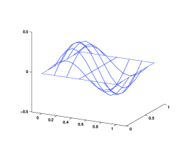
(b) Mode 2

Figure 9: Mode shape for a square plate without a crack. The mode shape is normalized with the maximum value.

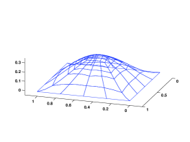
(a) Mode 1

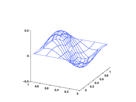
(b) Mode 2

Figure 10: Mode shape for a simply supported square plate with a crack $(c/a=0.2,~{}a/h=10,~{}T_{c}=600,~{}T_{m}=300,~{}n=0)$. The mode shape is normalized with the maximum value.

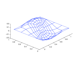
(a) c/a=0.2

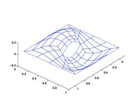
(b) c/a=0.4

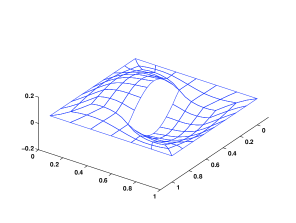
(c) c/a=0.6

Figure 11: Mode shape (second mode) for a simply supported square plate with different crack sizes $(a/h=10,~{}T_{c}=600,~{}T_{m}=300,~{}n=0)$. The mode shape is normalized with the maximum value.

Lastly, the effect of skewness of a simply supported and clamped square FGM plates in thermal environment is investigated. The thickness of the plate is taken as $a/h$=10 and the plate is assumed to have a center crack $c/a=0.2$. The results are shown in Tables 10 and 11 for various gradient indices and skew angles. It can be seen from Tables 10 and 11 that with increase in skew angle $\psi$, the linear frequency increases and with increase in gradient index $n$, the linear frequency decreases.

5 Conclusion

The linear free flexural vibration behavior of FGM plates with and without thermal environment is numerically studied using QUAD-8 shear flexible element. The formulation is based on first order shear deformation theory. The material is assumed to be temperature dependent and graded in the thickness direction according to the power-law distribution in terms of volume fractions of the constituents. The effective material properties are estimated using Mori-Tanaka homogenization method. Numerical experiments have been conducted to bring out the effect of gradient index, aspect ratio, crack length, thickness and boundary condition on the natural frequency of the FGM plate. From the detailed parametric study, it can be concluded that with increase in both the gradient index and crack length, the natural frequency decreases. In both cases, the decrease is due to stiffness degradation.

Acknowledgements

S Natarajan acknowledges the financial support of (1) the Overseas Research Students Awards Scheme; (2) the Faculty of Engineering, University of Glasgow, for period Jan. 2008 - Sept. 2009 and of (3) the School of Engineering (Cardiff University) for the period Sept. 2009 onwards.

S Bordas would like to acknowledge the financial support of the Royal Academy of Engineering and of the Leverhulme Trust for his Senior Research Fellowship entitled ”Towards the next generation surgical simulators” as well as the support of EPSRC under grants EP/G069352/1 Advanced discretisation strategies for ”atomistic” nano CMOS simulation and EP/G042705/1 Increased Reliability for Industrially Relevant Automatic Crack Growth Simulation with the eXtended Finite Element Method.

References

- [1] M. Koizumi, The concept of FGM, Ceram. Trans. Functionally Graded Mater. 34 (1993) 3–10.
- [2] M. Koizumi, FGM activities in Japan, Composites 28 (1–2) (1997) 1–4.
- [3] S. Suresh, A. Mortensen, Functionally graded metals and metal - ceramic composites: Part 2, thermomechanical behavior, Int. Mater. Rev. 42 (1997) 85–116.
- [4] J. Reddy, Z.-Q, Three dimensional thermomechanical deformations of functionally graded rectangular plates, European Journal of Mechanics A/Solids 20 (2001) 841–855.
- [5] S. Vel, R. Batra, Exact solutions for thermoelastic deformations of functionally graded thick rectangular plates, AIAA J 40 (2002) 1421–1433.
- [6] M. Kashtalyan, Three-dimensional elasticity solutions for bending of functionally graded plates, European Journal of Mechanics A/Solids 23 (2004) 853–864.
- [7] E. Pan, Exact solution for functionally graded isotropic elastic composite laminates, Journal of Composite Materials 37 (2003) 1903–1920.
- [8] I. Elishakoff, C. Gentilini, Three-dimensional flexure of rectangular plates made of functionally graded materials, ASME Journal of Applied Mechanics 72 (2005) 788–791.
- [9] K. Rohwer, R. Rolfes, Calculating 3d stresses in layered composite plates and shells, Mechanics of Composite Materials 34 (1998) 355–362.
- [10] V. Birman, L. Byrd, Modeling and analysis of functionally graded materials and structures, Applied Mechanics Reviews 60 (2007) 195–216.
- [11] L. Qian, R. Batra, L. Chen, Static and dynamic deformations of thick functionally graded elastic plates by using higher order shear and normal deformable plate theory and meshless local petrov galerkin method, Composites Part B: Engineering 35 (2004) 685–697.
- [12] H. Matsunaga, Stress analysis of functionally graded plates subjected to thermal and mechanical loadings, Composite Structures 87 (2009) 344–357.
- [13] A. Zenkour, Generalized shear deformation theory for bending analysis of functionally graded plates, Applied Mathematical Modeling 30 (2006) 67–84.
- [14] A. Zenkour, Benchmark trigonometric and 3D elasticity solutions for an exponentially graded thick rectangular plate, Archive of Applied Mechanics 77 (2007) 197–214.
- [15] G. Praveen, J. Reddy, Nonlinear transient thermoelastic analysis of functionally graded ceramic-metal plates, International Journal of Solids and Structures 35 (1998) 4457–4476.
- [16] J. Reddy, Analysis of functionally graded plates, International Journal for Numerical Methods in Engineering 47 (2000) 663–684.
- [17] E. Carrera, S. Brischetto, A. Robaldo, Variable kinematic model for the analysis of functionally graded material plate, AIAA J 46 (2008) 194–203.
- [18] J. Yang, H.-S. Shen, Dynamic response of initially stressed functionally graded rectangular thin plates, Composite Structures 54 (2001) 497–508.
- [19] J. Yang, H.-S. Shen, Vibration characteristic and transient response of shear-deformable functionally graded plates in thermal environment, Journal of Sound and Vibration 255 (2002) 579–602.
- [20] S. Vel, R. Batra, Three-dimensional exact solution for the vibration of functionally graded rectangular plates, Journal of Sound and Vibration 272 (2004) 703–730.
- [21] N. Sundararajan, T. Prakash, M. Ganapathi, Nonlinear free flexural vibrations of functionally graded rectangular and skew plates under thermal environments, Finite Elements in Analysis and Design 42 (2005) 152–168.
- [22] N. Sundararajan, T. Prakash, M. K. Singha, M. Ganapathi, Free vibration of functionally graded skew plates subjected to thermal environment, Journal of Aerospace Sciences and Technologies 57 (2005) 270–281.
- [23] M. Ganapathi, T. Prakash, N. Sundararajan, M. K. Singha, Large amplitude free flexural vibrations of functionally graded plates, Journal of Aerospace Sciences and Technologies 58 (2006) 60–64.
- [24] Y. Lee, X. Zhao, J. Reddy, Postbuckling analysis of functionally graded plates subject to compressive and thermal loads, Computer Methods in Applied Mechanics and Engineeringdoi:10.1016/j.cma.2010.01.008.
- [25] N. Sundararajan, M. Ganapathi, On the dynamic snap-through buckling of functionally graded spherical caps, Journal of Aerospace Sciences and Technologies 59 (2007) 223–227.
- [26] N. Sundararajan, T. Prakash, M. Ganapathi, On the vibrations and thermal buckling of functionally graded spherical caps, Journal of Aerospace Sciences and Technologies 59 (2007) 136–147.
- [27] N. Sundararajan, M. Ganapathi, Dynamic thermal buckling of functionally graded spherical caps, Journal of Engineering Mechanics: ASCE 134 (2007) 206–209.
- [28] S. Natarajan, P. Thiruvengadam, G. Manickam, Dynamic buckling of functionally graded spherical caps, AIAA J 44 (2006) 1097–1102.
- [29] T. Prakash, N. Sundararajan, M. Ganapathi, On the nonlinear axisymmetric dynamic buckling behavior of clamped functionally graded spherical caps, Journal of Sound and Vibration 299 (2007) 36–43.
- [30] P. Lynn, N. Kumbasar, Free vibrations of thin rectangular plates having narrow cracks with simply supported edges, Dev. Mech 4 (1967) 928–991.
- [31] B. Stahl, L. Keer, Vibration and stability of cracked rectangular plates., International Journal of Solids and Structures 8 (1972) 69–91.
- [32] R. Solecki, Bending vibration of rectangular plate with arbitrarly located rectilinear crack, Engineering Fracture Mechanics 22 (4) (1985) 687–695.
- [33] S. Khadem, M. Rezaee, Introduction of modified comparison functions for vibration analysis of a rectangular cracked plate., Journal of Sound and Vibration 236 (2) (2000) 245–258.
- [34] G. Wu, Y. Shih, Dynamic instability of rectangular plate with an edge cracked, Computers and Structures 84 (1-2) (2005) 1–10.
- [35] G. Qian, S. Gu, J. Jiang, A finite element model of cracked plates and application to vibration problems, Computers and Structures 39 (5) (1991) 483–487.
- [36] H. Lee, S. Lim, Vibration of cracked rectangular plates including transverse shear deformation and rotary inertia., Computers and Structures 49 (4) (1993) 715–718.
- [37] T. Belytschko, R. Gracie, G. Ventura, A review of extended/generalized finite element methods for material model, Modelling and Simulation in Materials Science and Engineering 17 (4) (2009) 1–24.
- [38] G. R. Liu, K. Y. Dai, T. T. Nguyen, A smoothed finite element for mechanics problems, Computational Mechanics 39 (6) (2007) 859–877. doi:10.1007/s00466-006-0075-4.
- [39] G. Liu, T. Nguyen-Thoi, K. Lam, A novel alpha finite element method (FEM) for exact solution to mechanics problems using triangular and tetrahedral elements, Computer Methods in Applied Mechanics and Engineering 197 (2008) 3883–3897.
- [40] H. Nguyen-Xuan, T. Rabczuk, S. Bordas, J. F. Debongnie, A smoothed finite element method for plate analysis, Computer Methods in Applied Mechanics and Engineering 197 (2008) 1184–1203.
- [41] G. Liu, T. Nguyen-Thoi, H. Nguyen-Xuan, K. Lam, A node based smoothed finite element method (NS-FEM) for upper bound solution to solid mechanics problems, Computers and Structures 87 (2009) 14–26.
- [42] S. P. A. Bordas, S. Natarajan, On the approximation in the smoothed finite element method (sfem), International Journal for Numerical Methods in Engineering 81 (2010) 660–670. doi:10.1002/nme.2713.
- [43] V. P. Nguyen, T. Rabczuk, S. Bordas, Meshless methods: A review and computer implementation aspects, Mathematics and Computers in Simulation 79 (2008) 763–813. doi:10.1016/j.matcom.2008.01.003.
- [44] A. Ferreira, R. Batra, C. Roque, L. Qian, R. Jorge, Natural frequencies of functionally graded plates by a meshless method, Composite Structures 75 (2006) 593–600.
- [45] D. Gilhooley, R. Batra, J. Xiao, M. McCarthy, J. G. Jr., Analysis of thick functionally graded plates by using higher-order shear and normal deformable plate theory and mlpg method with radial basis functions, Composite Structures 80 (2007) 539–552.
- [46] J. Yang, Y. Chen, Free vibration and buckling analyses of functionally graded beams with edge cracks, Composite Structures 83 (2008) 48–60.
- [47] S. Kitipornchai, L.-L. Ke, J. Yang, Nonlinear vibration of edge cracked functionally graded timoshenko beams, Journal of sound and vibration 324 (2009) 962–982.
- [48] G. Prathap, B. Naganarayana, B. Somashekar, A field consistency analysis of the isoparametric eight-noded plate bending elements, Computers and Structures 29 (1988) 857–874.
- [49] M. Ganapathi, T. Varadan, B. Sarma, Nonlinear flexural vibrations of laminated orthotropic plates, Computers and Structures 39 (1991) 685–688.
- [50] T. Mori, K. Tanaka, Average stress in matrix and average elasticenergy of materials with misfitting inclusions, Acta Metallurgica 21 (1973) 571–574.
- [51] Y. Benvensite, A new approach to the application of mori–tanaka’s theory in composite materials, Mechanics of Materials 6 (1987) 147–157.
- [52] Z.-Q. Cheng, R. Batra, Three dimensional thermoelastic deformations of a functionally graded elliptic plate, Composites Part B: Engineering 2 (2000) 97–106.
- [53] H. Hatta, M. Taya, Effective thermal conductivity of a misoriented short fiber composite, Journal of Applied Physics 58 (1985) 2478–2486.
- [54] B. Rosen, Z. Hashin, Effective thermal expansion coefficients and specific heats of composite materials, International Journal of Engineering Science 8 (1970) 157–173.
- [55] J. Reddy, C. Chin, Thermomechanical analysis of functionally graded cylinders and plates, Journal of Thermal Stresses 21 (1998) 593–629.
- [56] L. Wu, Thermal buckling of a simply supported moderately thick rectangular FGM plate, Composite Structures 64 (2004) 211–218.
- [57] S. Rajasekaran, D. Murray, Incremental finite element matrices, ASCE Journal of Structural Divison 99 (1973) 2423–2438.
- [58] D. Makhecha, B. Patel, M. Ganapathi, Transient dynamics of thick skew sandwich laminates under thermal/mechanical loads, Journal of Reinforced Plastics and Composites 20 (2001) 1524–1545.
- [59] M. Singh, T. Prakash, M. Ganapathi, Finite element analysis of functionally graded plates under transverse load, Finite Elements in Analysis and Design 47 (2011) 453–460.
- [60] K. Liew, K. Hung, K. Lim, A solution method for analysis of cracked plates under vibration, Engineering Fracture Mechanics 48 (1994) 393–404.
- [61] S. Natarajan, P. M. B. Villafranca, S. P. Bordas, T. Rabczuk, Linear free flexural vibration of cracked isotropic plates using the extended finite element method, Algorithms Article in review.
- [62] X.-L. Huang, H.-S. Shen, Nonlinear vibration and dynamic response of functionally graded plates in thermal environments, International Journal of Solids and Structures 41 (2004) 2403–2427.