Dynamical chaos in the problem of magnetic jet collimation

Abstract

We investigate dynamics of a jet collimated by magneto-torsional oscillations. The problem is reduced to an ordinary differential equation containing a singularity and depending on a parameter. We find a parameter range for which this system has stable periodic solutions and study bifurcations of these solutions. We use Poincaré sections to demonstrate existence of domains of regular and chaotic motions. We investigate transition from periodic to chaotic solutions through a sequence of period doublings.

1 Introduction

Many quasars and active galactic nuclei are connected with long thin collimated outbursts – jets. When observed with high angular resolution, these jets show structure with bright knots separated by relatively dark regions. A mechanism of collimation of such jets is still questionable. Magnetic collimation of jets was first considered by Bisnovatyi-Kogan, Komberg & Fridman (1969). In the paper of Bisnovatyi-Kogan (2007) magnetic collimation resulting from torsional oscillations of a cylinder with elongated magnetic field and periodically distributed initial rotation around the cylinder axis was considered (Fig. 1). The stabilizing azimuthal magnetic field is created here by torsional oscillations. An approximate simplified model was developed, and an ordinary differential equation was derived describing the process of dynamic stabilization. The interval of parameters, for jet stabilization to occur, was estimated qualitatively.

The ordinary differential equation under consideration is a non-linear non-autonomous time-periodic second order equation with a singularity in the right hand side. The equation contains one dimensionless parameter $D$, which summarizes the information about the magnetic field, amplitude and frequency of oscillations, radius of the jet, its spatial period along the jet axis, and sound speed in the jet matter. Here we investigate analytically and numerically the structure of the phase space of this equation, which has a very peculiar character and contains chaotic solutions as well as quasi-periodic and periodic regular solutions.

The paper is organized as follows. In section 2 we describe in more detail the mechanism of jet collimation by magneto-torsional oscillations and the dynamic confinement equation. In section 3 we discuss the main types of solutions of this equation. In section 4 we investigate analytically and numerically the dynamics of the system for large radii. In section 5 we construct Poincaré sections for different values of parameter $D$. In section 6 we study periodic solutions undergoing a sequence of period doublings at values of parameter $D=D_{n}$, $n=$1,2,3,…, when $D$ increases. In section 7 we discuss a possible mechanism of jet formation with a variable direction of angular velocity and estimate the value of $D$ for astrophysical jets.

We have found that stable periodic solutions disappear after an infinite cascade of period doublings. In the problem of period doubling the limiting constant $q$ for values $[D_{n}-D_{n-1}]/[D_{n+1}-D_{n}]$ is usually considered. For large $n$ the constant $q$ equals to Feigenbaum constant $F=4.6692...$ for dissipative systems, see Feigenbaum (1980), and $FH=8.721...$ for Hamiltonian systems, see Greene et al. (1981). In our work we obtain that $q$ is approaching 8.72, in agreement with the expected behaviour for Hamiltonian systems.

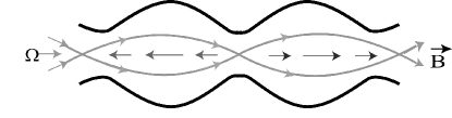
Figure 1: Jet confinement by magneto-torsional oscillations (qualitative picture).

2 Dynamic confinement of jets by magnetotorsional oscillations

We consider jet stabilization by pure magneto-hydrodynamic mechanism associated with torsional oscillations. Jets are relativistically moving objects, and the whole analysis of present paper takes place at the rest frame of the bulk motion of the jet. We suggest that matter in the jet is rotating, and different parts of the jet rotate in different directions (see Fig. 1). Such distribution of rotational velocity produces azimuthal magnetic field, which prevents the disruption of the jet. The jet is represented by a periodic, or quasi-periodic structure along the axis, and its radius oscillates with time all along the axis. Space and time periods of oscillations depend on the conditions of jet formation: the length-scale, the amplitude of the rotational velocity, and the strength of the magnetic field. Time period of oscillations can be calculated in the framework of the dynamical model. The range of parameters, for which dynamical stabilization occurs, should also be inferrible from the model. Two-dimensional non-stationary MHD calculations are needed to solve the problem numerically. A very simplified model of this phenomenon was constructed by Bisnovatyi-Kogan (2007). This model allowed to confirm the possibility of such stabilization, to estimate the interval of parameters when it takes place and to establish the connection between time and space scales, magnetic field strength, and amplitude of rotational velocity.

Let us consider a long cylinder with magnetic field directed along its axis. This cylinder will expand without limit under the action of pressure and magnetic forces. It is possible, however, that a limiting value of the cylinder radius could be reached in a dynamic state, when the whole cylinder undergoes magneto-torsional oscillations. Such oscillations produce a toroidal field (magnetic field lines are frozen into matter), which prevents radial expansion. There is therefore a competition between the induced toroidal field, compressing the cylinder in the radial direction, and the gas pressure, together with the field along the cylinder axis (poloidal), tending to increase its radius. During magneto-torsional oscillations there are phases when either compression or expansion force prevails, and, depending on the input parameters, there are three possible kinds of behaviour of such a cylinder that has negligible self-gravity.

(1) The oscillation amplitude is low, so the cylinder suffers unlimited expansion (no confinement).

(2) The oscillation amplitude is high, so the pinch action of the toroidal field destroys the cylinder and leads to the formation of separated blobs.

(3) The oscillation amplitude is moderate, so the cylinder, in absence of any damping, survives for an unlimited time, and its parameters (radius, density, magnetic field, etc.) change periodically, or quasi-periodically, or chaotically in time.

These phenomena can be described in general by the system of axially symmetric MHD equations (Bisnovatyi-Kogan, 2007). The system of equations was simplified in the paper of Bisnovatyi-Kogan (2007) to investigate the most important property of dynamical competition between different forces in order to check for the possibility of dynamical confinement. A profiling procedure was used for this purpose. In particular, gravity in the direction of the cylinder axis was neglected, approximate uniform density along the radius was assumed, and adiabatic case with polytropic equation of state was considered. Approximate system allowed to investigate linear oscillations (around the equilibrium state in presence of gravity) of infinite, self-gravitating cylinder with uniform magnetic field and rotation along its axis.

For further simplification gravity was neglected, because in a relativistic jet the self-gravitating force is expected to be much lower than the magnetic and pressure forces. In this approximation we have the following feature of problem. Without gravity the equilibrium static state of the cylinder does not exist. But it turns out that nevertheless bounded solutions exist, where cylinder radius oscillates and remains finite (dynamic confinement). Confinement by magneto-torsional oscillations is therefore physically realizable. Similar situation is observed for instance in the simulations of electron-positron discharges in the polar cap of pulsar – the pair cascade settles down to a stable state where it has a limiting cycle type of behaviour (Timokhin, 2010).

After considerable simplifications, details of which may be found in the paper of Bisnovatyi-Kogan (2007), the equation, describing the magneto-torsional oscillations of a long cylinder, takes the following form:

$$\frac{d^{2}\,y}{d\,\tau^{2}}=\frac{1-D\,\sin^{2}\,\tau}{y}.$$ (1)

This equation describes approximately time dependence of the outer radius of the cylinder $R(t)$ in the symmetry plane, where the rotational velocity remains zero. The cylinder has magnetic field $B_{z}(t)$, isothermal equation of state of matter $P=K\rho$, maximal amplitude of the angular velocity of oscillations $\Omega_{0}$, and angular frequency of oscillations $\omega$. The oscillating cylinder has a periodic structure along the $z$ axis, with space period $z_{0}$. The nodes with zero amplitude of oscillations are situated at $z=\pm n\frac{z_{0}}{2}$, and the oscillations with maximal angular amplitude $\Omega_{0}$ are situated at $z=\frac{z_{0}}{4}\pm n\frac{z_{0}}{2}$, $n=0,1,2...$. Axial motion of the matter in the cylinder is neglected, and density $\rho(t)$ is supposed to be uniform along the radius. Under these conditions the equations for conservation of mass and magnetic flux (we assume infinite electrical conductivity) determine the constant values $C_{m}$ and $C_{b}$:

$$\rho\,R^{2}=C_{m}=\rho_{0}R_{0}^{2},\quad B_{z}\,R^{2}=C_{b}=B_{z,0}R_{0}^{2},$$ (2)

where $\rho_{0}$, $R_{0}$, and $B_{z,0}$ are some characteristic values. The dimensionless variables and the parameter $D$ in (1) are defined as

$$\tau=\omega\,t,\quad y=\frac{R}{R_{0}},$$ (3)

$$\hbox{with}\quad R_{0}=\frac{\sqrt{K}}{\omega},\quad D=\frac{1}{2\pi KC_{m}}\left(\frac{C_{b}\Omega_{0}}{z_{0}\omega}\right)^{2}.$$

The frequency of oscillations $\omega$ may be represented as

$$\omega=\alpha_{n}kV_{A}=\alpha_{n}\frac{B_{z,0}}{z_{0}}\sqrt{\frac{\pi}{\rho_{0}}},$$ (4)

where $k$ is the wave number, $k=2\pi/z_{0}$, and $V_{A}$ is the Alfven velocity, $V_{A}=B_{z,0}/\sqrt{4\pi\rho_{0}}$; $\alpha_{n}<1$ is a coefficient determining the frequency of non-linear Alfven oscillations, which are identical to magneto-torsional oscillations under investigation. In our problem there are no static solutions. In a balanced non-compressible cylinder the frequency of magneto-torsional oscillations is defined by (4) with $\alpha_{n}=1$.

3 General types of solutions of dynamic confinement equation

Equation (1) was solved numerically in the paper of Bisnovatyi-Kogan (2007) for different values of parameter $D$, and fixed initial conditions $y(0)=1,y^{\prime}(0)=0$. The following three regimes of the behaviour were found in these calculations.

(1) $D<2.1$ The oscillation amplitude is low, so the cylinder should suffer unlimited expansion (no confinement). This regime corresponds to small $D$. For example at $D=2$ there is no confinement, and radius grows to infinity after several low-amplitude oscillations, Fig. 2.

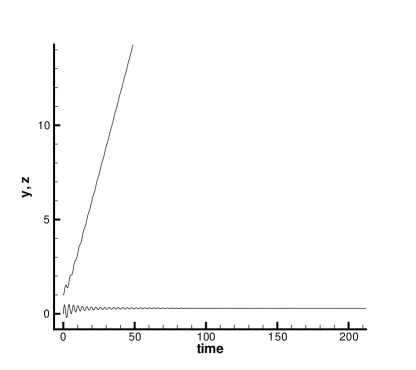
Figure 2: Time dependence of non-dimensional radius $y$ (upper curve), and non-dimensional velocity $z=y^{\prime}$ (lower curve), for $D=2.0$.

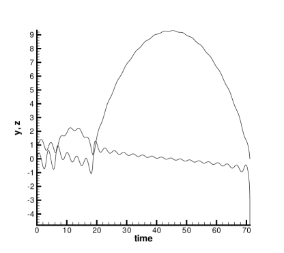
Figure 3: Time dependence of non-dimensional radius $y$ (upper curve), and non-dimensional velocity $z=y^{\prime}$ (lower curve), for $D=2.4$.

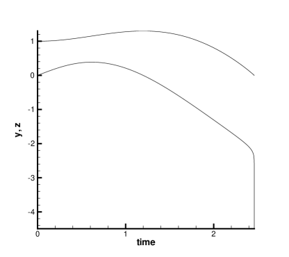
Figure 4: Time dependence of non-dimensional radius $y$ (upper curve), and non-dimensional velocity $z=y^{\prime}$ (lower curve), for $D=3.0$.

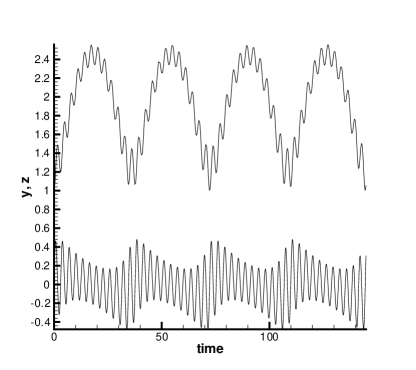
Figure 5: Time dependence of non-dimensional radius $y$ (upper curve), and non-dimensional velocity $z=y^{\prime}$ (lower curve), for $D=2.1$.

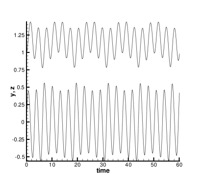
Figure 6: Time dependence of non-dimensional radius $y$ (upper curve), and non-dimensional velocity $z=y^{\prime}$ (lower curve), for $D=2.25$.

(2) $D>2.28$ The oscillation amplitude is too high, so the pinch action of the toroidal field destroys the cylinder, and leads to formation of separated blobs. The calculations show (Bisnovatyi-Kogan, 2007), that at $D=2.28$ and larger, the radius finally goes to zero with time, but with different behaviour, depending on $D$. At $D$ between 2.28 and 2.9 time dependence of the radius $y$ may be very complicated, consisting of low-amplitude and large-amplitude oscillations, which finally decay to zero. The time at which radius becomes zero depends on $D$ in a rather peculiar way, and it may happen at $\tau<100$, like at $D=2.4$ (Fig. 3), $2.6$, or at $\tau\sim 10^{7}$ like at $D=2.5$ (in the last case the radius passes through very large values and then returns back to zero). For $D=3$ and larger the solution is very simple: the radius goes to zero at $\tau<2.5$, before the return of the right hand side of (1) to a positive value, Fig. 4.

(3) For the intermediate interval $2.1<D<2.28$ the radius is not growing to infinity, but is oscillating around some average value. The cylinder survives for a unlimited time, and its parameters (radius, density, magnetic field, etc.) change periodically or quasi-periodically in time, Figs 5, 6.

The above results from the paper of Bisnovatyi-Kogan (2007) have been obtained for solutions only with initial radius $y_{0}=1$. The solutions at moderate $D$ are not pure periodic, but it is not clear from the figures, whether are they regular or chaotic.

In the current paper we investigate the solutions of (1) for different values of $D$ and different initial radii $y_{0}$, mainly for moderate $D$’s. Solutions of principal interest are those that do not go neither to 0 nor to infinity. Such solutions correspond to stabilized jets. We use averaging method and Poincaré sections to investigate the properties of these solutions.

4 Dynamics for large radii

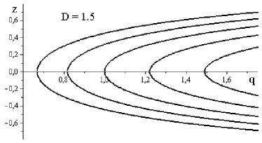
Figure 7: Phase curves of the system with Hamiltonian (9) for $D=1.5$, and ${\cal H}=-0.1,-0.05,0,0.05,0.1$.

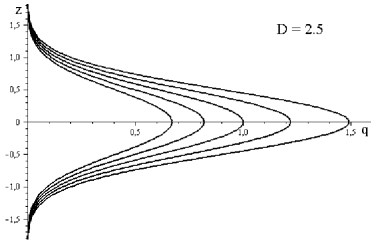
Figure 8: Phase curves of the system with Hamiltonian (9) for $D=2.5$, and ${\cal H}=-0.1,-0.05,0,0.05,0.1$.

Let us denote $z=y^{\prime}\equiv dy/d\tau$. Equation (1) is equivalent to the system

$$y^{\prime}=z,\quad z^{\prime}=\frac{1-D\,\sin^{2}\,\tau}{y}.$$ (5)

We consider a motion for large values of $y$. In this limit let us introduce a small number $\varepsilon$ and denote $q=\varepsilon y$. We will assume that $y\sim 1/\varepsilon$, and therefore $q\sim 1$. The equation system for $q,\,z$ is

$$q^{\prime}=\varepsilon z,\quad z^{\prime}=\varepsilon\frac{1-D\,\sin^{2}\,\tau}{q}.$$ (6)

This is a Hamiltonian system with Hamiltonian

$$\varepsilon H=\varepsilon\left[\frac{z^{2}}{2}-(1-D\sin^{2}\tau)\ln q\right]$$ (7)

and equations of motion

$$q^{\prime}=\varepsilon{\partial H}/{\partial z},\quad z^{\prime}=-\varepsilon{\partial H}/{\partial q}.$$ (8)

For small $\varepsilon$ the variables $q,z$ are changing slowly with respect to changing of $\tau$. The averaging method (Bogolyubov & Mitropolskii, 1961) prescribes to average Hamiltonian (7) over the fast variable $\tau$ for an approximate description of the behaviour of the slow variables $q,z$. We get the averaged Hamiltonian

$$\varepsilon{\cal H}=\varepsilon\left[\frac{z^{2}}{2}-\left(1-\frac{D}{2}\right)\ln q\right].\\$$ (9)

Phase curves of the system with Hamiltonian (9) for $D<2$, and for $D>2$ are shown in Figs 7 and 8, respectively.

If $D<2$, then for Hamiltonian (9) $q(t)$ and $y(t)\to\pm\infty,z(t)\to\pm\infty$ as $t\to\pm\infty$ for all solutions of the averaged system. This situation corresponds to the unlimited expansion of the jet (no collimation). If $D>2$, then $q(t)$ and $y(t)\to 0,z(t)\to\pm\infty$ as $t\to\mp\tau_{*}$, where $\tau_{*}$ is some finite moment of time that depends on the chosen solution. This corresponds to strong initial amplitude of pulsations leading to the fragmentation of the jet into separate clumps.

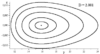
Figure 9: Poincaré section near the stable fixed point, $z=y^{\prime}\equiv dy/d\tau$, $D=2.001$. One periodic and five quasi-periodic solutions are shown. This figure is constructed numerically by solutions of equations (5). Difference between curves in this figure and phase curves from approximate formula (12) is about thickness of line on figure, therefore we do not show the latter curves here.

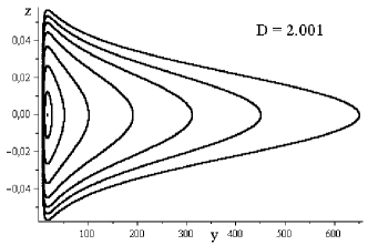
Figure 10: Poincaré section for $D=2.001$. This figure is constructed numerically by solutions of equations (5). Difference between curves in this figure and phase curves from approximate formula (12) is about thickness of line on figure, therefore we do not show the latter curves here.

Solutions of the averaged system describe approximately the solutions of the exact system for large values of $y$ provided that $(D-2)$ is not small.

It turns out that for small $(D-2)>0$ the exact system has a stable periodic solution, which is described approximately by the formulas

$$y=\frac{1}{2\sqrt{D-2}}-\frac{1}{2}\sqrt{D-2}\cos 2\tau,\quad z=\sqrt{D-2}\sin 2\tau.$$ (10)

(see Appendix). In the Poincaré section $\{\tau=0\,{\rm mod}\,\,\pi\,\}$ this solution is depicted as a fixed point of the Poincaré return map. This fixed point is located on the axis $z=0$, its $y$-coordinate is given approximately by the formula

$$y=\frac{1}{2\sqrt{D-2}}-\frac{1}{2}\sqrt{D-2}.$$ (11)

This fixed point is surrounded by a family of invariant curves of the Poincaré return map. The approximate equation for these invariant curves is

$$\frac{1}{2}z^{2}+\frac{1}{16y^{2}}+\frac{1}{2}(D-2)\ln y={\rm const}$$ (12)

(see Appendix). The fixed point and surrounding it invariant curves are shown in Fig. 9 for $D=2.001$.

The Poincaré sections are constructed numerically in this paper. For the same value of D, we solve equations (5) for different initial $y_{0}$ and $z_{0}$. During the numerical integration of equations, we mark moments $\tau=0\,\,{\rm mod}\,\,\pi$. For each integration, we put the points on the plane $(y,z)$ at the moments $\tau=0\,\,{\rm mod}\,\,\pi$. The regular oscillations are represented by closed lines (invariant curves) on the Poincaré maps: closed curves correspond to regular quasi-periodic solutions, points in the centers of families of such curves correspond to stable regular periodic solutions. Chaotic behaviour fills regions of finite area with dots on the Poincaré maps.

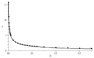
Figure 11: $y$-coordinate of the stable fixed point as a function of $D$. In this figure the separated points are obtained by numerical calculations, the curve is plotted analytically with formula (11).

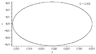
Figure 12: Phase trajectory corresponding to periodic solution for $D=2.001$; initial data $y(0)=15.8034860625$, $z(0)=0$. Phase trajectory is constructed by numerical solution of equations (5) at given initial values and putting all dots of solution on the plane $(y,z)$.

For this value of $D=2.001$ the family of invariant curves covers rather a big domain in the Poincaré section, see Fig. 10. For initial conditions on the invariant curves the solution of the equation (1) is represented by quasi-periodic functions of $\tau$. The values of $y$-coordinate of the fixed point, obtained theoretically (see (11)) and numerically, are shown in Fig. 11.

One can see that the obtained asymptotic expression for the coordinates (radii) of the stable fixed points works very well even for $D$ not very close to 2 (and therefore when $y$ is not very big). The projection onto the plane $y,z$ (in another words, phase trajectory) of the periodic solution corresponding to the fixed point in Fig. 9 is shown in Fig. 12.

5 Poincaré sections for different values of parameter $D$

In order to find bounded regular solutions we have constructed a Poincaré section for the system (5) for $\tau=0\,\,{\rm mod}\,\,\pi$ for different values of parameter $D$. We use such construction of the Poincaré section because the right-hand side of the equation (1) is a periodic function of $\tau$ with period $\pi$. Recall that in Bisnovatyi-Kogan (2007) such solutions with $y_{0}=1$ were found to exist only for $\sim 2.1<D<\sim 2.28$. We will concentrate here on the behaviour of the invariant curves on the Poincaré section around the stable fixed point of the Poincaré return map, and on the transition to chaotic behaviour in this region with increasing of parameter $D$.

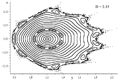
Figure 13: Poincaré section for $D=2.15$. Central point corresponds to a stable periodic solution of period $\pi$.

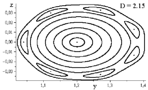
Figure 14: Zoom of the part of Fig. 13: islands on Poincaré section for $D=2.15$.

In Figs 13, 14 the Poincaré section for $D=2.15$ is presented. The closed invariant curves cross axis $z=0$ in the interval $0.8\sim<y_{0}<\sim 1.80$. Outside this interval solutions of equations (5) show non-regular chaotic behaviour, with unbounded trajectories. Central point in Fig. 13 corresponds to the periodic solution with period $\pi$. One can see a chain of seven stability islands, centres of which determine periodic solution with period $7\pi$; zoom of this chain is presented in Fig. 14. In Fig. 13 one can also see a chain of fifteen stability islands, centres of these islands correspond to periodic solution with period $15\pi$.

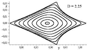
Figure 15: Invariant curves on Poincaré section for $D=2.25$. The stable fixed point in the centre has coordinates $y=0.887$, $z=0$.

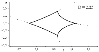
Figure 16: Appearance of chaos on Poincaré section for $D=2.25$.

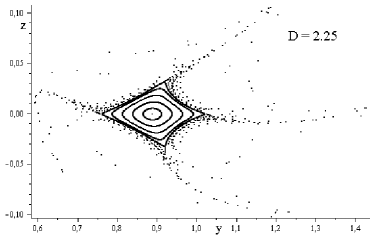
Figure 17: Invariant curves and chaotic trajectories on Poincaré section for $D=2.25$.

Invariant curves around the periodic solution for $D=2.25$ are plotted in Fig. 15. In Fig. 16 the appearance of a chaotic solution is shown. The last shown invariant curve corresponds to the solution with initial values $y(0)=0.757$, $z(0)=0$, while the solution with $y(0)=0.756$, $z(0)=0$ is already chaotic. In Fig. 17 a general picture of regular and chaotic trajectories is represented.

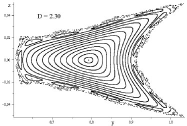
Figure 18: Invariant curves and chaotic trajectories on Poincaré section for $D=2.30$. Central point corresponds to a stable periodic solution of period $\pi$.

Invariant curves and chaotic trajectories on the Poincaré section are plotted for $D=2.30$ in Fig. 18, and for $D=2.35$ in Fig. 19.

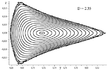
Figure 19: Invariant curves and chaotic trajectories on Poincaré section for $D=2.35$. Central point corresponds to a stable periodic solution of period $\pi$.

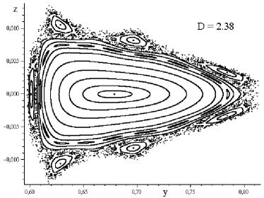
Figure 20: Invariant curves and chaotic trajectories on Poincaré section for $D=2.38$. Central point corresponds to a stable periodic solution of period $\pi$.

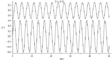
Figure 21: Time dependence of non-dimensional radius $y$ (upper curve) and non-dimensional velocity $z=y^{\prime}$ (lower curve) for periodic solution of period $\pi$, see central point in Fig. 20; $D=2.38$.

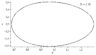
Figure 22: Phase trajectory in the plane $y,z$ for periodic solution of period $\pi$, see central point in Fig. 20; $D=2.38$.

The case $D=2.38$ is represented in Fig. 20. Layers with both regular and chaotic trajectories are situated around periodic solutions. In Figs 21, 22 time evolution $y(\tau)$, $z(\tau)$ and phase trajectory in the plane $y,z$ are shown for a periodic solution with period $\pi$.

6 Transition to chaos via cascade of period doublings

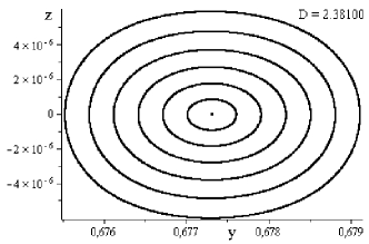
Figure 23: Poincaré section for $D=2.38100$.

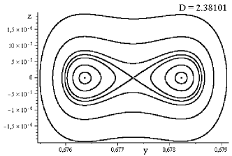
Figure 24: Poincaré section for $D=2.38101$. This value of $D$ corresponds to first period doubling. The left central point maps to the right central point after time $\pi$, then visa versa. Compare with Fig. 23, where Poincaré section just before this doubling is shown.

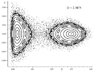
Figure 25: Poincaré section after first period-doubling; $D=2.3875$. Two points in centres of concentric curves correspond to the periodic solution of the period $2\pi$.

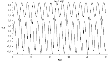
Figure 26: Time dependence of non-dimensional radius $y$ (upper curve) and non-dimensional velocity $z=y^{\prime}$ (lower curve) for the periodic solution of period $2\pi$, see points in Fig. 25; $D=2.3875$.

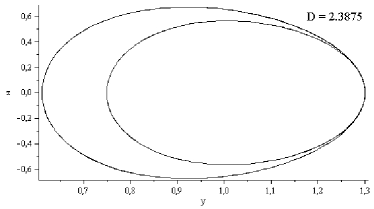
Figure 27: Phase trajectory in the plane $y,z$ for periodic solution of period $2\pi$, see points in Fig. 25; $D=2.3875$.

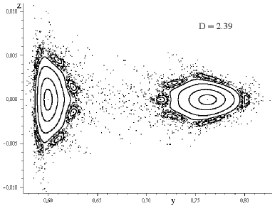
Figure 28: Poincaré section for $D=2.39$. Two points in the centres of concentric curves correspond to a periodic solution of period $2\pi$.

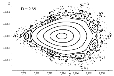
Figure 29: Zoom of left part of right island in Fig. 28. The island at the Poincaré section for $D=2.39$. The point in the centre of the island corresponds to the periodic solution of the period $12\pi$.

With increasing $D$ the stable periodic solution considered in Sections 4 and 5 loses its stability via period doubling bifurcation. The first period doubling occurs at $D_{1}=2.38101$. At this value $D_{1}$ the solution with period $\pi$ becomes unstable, and a stable periodic solution of period $2\pi$ appears.

The subsequent points of period doubling $D_{1}$, $D_{2}$, … can be found by constructing Poincaré sections for different values of $D$. In Fig. 23 the central part of the Poincaré section for value of $D$ before the first bifurcation is shown. In Fig. 24 the central part of the Poincaré section for value $D$ soon after doubling is shown. Periodic solution with period $\pi$ is now unstable, but there is a stable periodic solution of period $2\pi$. On Poincaré section this solution is represented by two points surrounded by closed curves (Fig. 24). Under one iteration of Poincaré return map the left point and surrounding it curves are mapped, respectively, onto right point and surrounding it curves, and vice versa. With increasing $D$ the distance between the points of periodic solution on Poincaré section increases.

In Fig.25 the Poincaré section for a slightly greater value of $D$, namely $D=2.3875$ is shown. In Figs 26, 27 time evolution $y(\tau)$, $z(\tau)$ and phase trajectory in $y,z$ plane for the periodic solution with period $2\pi$ are shown.

At $D_{2}=2.410172$ the periodic solution with period $2\pi$ becomes unstable, and a stable periodic solution of period $4\pi$ appears. The following doubling points found by the Poincaré section construction are:

$$D_{1}\simeq 2.38101,\quad\pi\rightarrow 2\pi,$$

$$D_{2}\simeq 2.410172,\quad 2\pi\rightarrow 4\pi,$$

$$D_{3}\simeq 2.4137115,\quad 4\pi\rightarrow 8\pi,$$

$$D_{4}\simeq 2.4141168,\quad 8\pi\rightarrow 16\pi,$$

$$D_{5}\simeq 2.4141633,\quad 16\pi\rightarrow 32\pi.$$

The values $D_{1}$, $D_{2}$, $D_{3}$, $D_{4}$ have also been obtained with the help of of AUTO-07P: Continuation and Bifurcation Software for Ordinary Differential Equations (Doedel & Oldeman (2009), http://cmvl.cs.concordia.ca/auto/).

According to Greene et al. (1981) the limiting constant

$$q=\frac{D_{n}-D_{n-1}}{D_{n+1}-D_{n}}$$ (13)

should for large $n$ approach the constant $FH=8.721$ for Hamiltonian systems. We obtain the following values:

$$q_{123}=\frac{D_{2}-D_{1}}{D_{3}-D_{2}}\simeq 8.24,$$

$$q_{234}=\frac{D_{3}-D_{2}}{D_{4}-D_{3}}\simeq 8.73,$$

$$q_{345}=\frac{D_{4}-D_{3}}{D_{5}-D_{4}}\simeq 8.72.$$

We conclude that this behaviour agrees with the expected one for Hamiltonian systems, despite of the additional symmetry $z\rightarrow-z$, $t\rightarrow-t$.

We can find approximately the value of parameter $D_{\infty}$ for which stable periodic solutions disappear after an infinite cascade of period doublings using the value $q\simeq 8.721$:

$$D_{\infty} = D_{4}+(D_{5}-D_{4})+(D_{6}-D_{5})+(D_{7}-D_{6})+...$$ (14)

$$= D_{4}+(D_{5}-D_{4})+\frac{D_{5}-D_{4}}{q}+\frac{D_{5}-D_{4}}{q^{2}}+...$$

$$= D_{4}+\frac{D_{5}-D_{4}}{1-1/q}\simeq 2.4141693.$$

In Table 1 we summarize the figures of the present article.

Table 1: Values of parameter $D$ and numbers of corresponding figures.

Values of parameter $D$	Numbers of figures
1.5	7
2.0	2
2.001	9, 10, 12
2.1	5
2.15	13, 14
2.25	6, 15, 16, 17
2.30	18
2.35	19
2.38	20, 21, 22
2.38100	23
2.38101	24
2.3875	25, 26, 27
2.39	28, 29
2.4	3
2.5	8
3.0	4

7 Discussion

In this section we would like to address the issue of a jet angular velocity oscillations generation. Jets are associated with accretion and consist of ejected matter from accretion disc. Jet matter inherits angular momentum from the accretion disc matter.

The jet matter may have a periodically (or quasi-periodically) varying sign of the angular momentum of the accretion disc matter around a supermassive black hole. In a dense stellar cluster around the SMBH, the accretion disc can change its direction of rotation due to different sign of the angular momentum of matter of the disrupted accreting stars. In this situation the magneto-torsional oscillations should be inevitably generated in the outflowing jets.

In the case, when stellar cluster is rotating, the disrupted stars will preserve the excess of the angular momentum, and the jet may rotate, and there should be oscillations of the angular velocity around the regular rotation. The presence of these oscillations will lead to effects similar to ones described in our model. But the presence of regular rotation makes the physical picture of phenomenon more complicated, because of the centrifugal force created by regular rotation and leading to jet expansion in radial direction.

In the framework of our model we have demonstrated that for a narrow range of the parameter $D$ the cylinder radius remains finite for a long time. This can potentially lead to a long-live jets. Due to complicated nature of the problem, we can not estimate the number of jets collimated by this mechanism. In the case of $D<2$ the jet collimation does not occur. We can tell that if $D>2$ then jet exists in a continuous form or in the form of blobs, both configurations corresponding to observations.

We can estimate value of $D$

$$D=\frac{1}{2\pi KC_{m}}\left(\frac{C_{b}\Omega_{0}}{z_{0}\omega}\right)^{2}$$ (15)

in the following way:

$$\Omega_{0}\simeq\frac{c}{R_{0}},\quad z_{0}\simeq R_{0},\quad C_{m}\simeq\rho_{0}R_{0}^{2},\quad C_{b}\simeq B_{z,0}R_{0}^{2},$$ (16)

$$\omega\simeq\alpha_{n}\frac{B_{z,0}}{z_{0}}\sqrt{\frac{\pi}{\rho_{0}}},\quad K\simeq\frac{c^{2}}{A}.$$ (17)

Here $c$ is the speed of light, $R_{0}$, $\rho_{0}$ and $B_{z,0}$ are some characteristic values of length, density and magnetic field correspondingly, $A$ is the non-dimensional constant. We obtain:

$$D=\frac{A}{2\pi^{2}\alpha_{n}^{2}}.$$ (18)

For estimation of $A$ we can write: $P=nkT$, $n=\frac{\rho_{0}}{m_{p}}$, where $P$ is the pressure, $n$ is the concentration, $T$ is the temperature, $m_{p}$ is the proton mass, $k$ is the Boltzmann constant. Comparing with $P=K\rho_{0}$ we obtain:

$$A=\frac{m_{p}c^{2}}{kT}.$$ (19)

For estimation in a nonlinear regime of oscillations we can put $\alpha_{n}^{2}=0.1$ (see Bisnovatyi-Kogan (2007)).

We see that for a sufficiently large proton loading ($A>1$) we can have $D>2$.

Appendix A Approximate formulas for periodic solutions and invariant curves

We will use a standard approach for the averaging method. We will make a canonical time-periodic transformation of variables such that the Hamiltonian for the new variables will not depend on time in the principal approximation. Discarding small time-depending terms in the Hamiltonian we will get a Hamiltonian for some autonomous system. We will find an equilibrium position of this system. The exact system in the new variables has a periodic solution close to this equilibrium position. Then we will find formulas for this periodic solution in the old variables making use of the formulas for the transformation of variables.

We will construct the required transformation of variables as a composition of several transformations of variables. In the system with Hamiltonian (7) we make a canonical transformation of variables $(q,z)\mapsto(\bar{q},\bar{z})$ with a generating function of the form

$$q\bar{z}+\varepsilon S_{1}(q,\bar{z},\tau).$$ (20)

The old variables $(q,z)$ and the new variables $(\bar{q},\bar{z})$ are related via formulas

$$z=\bar{z}+\varepsilon\frac{\partial S_{1}}{\partial q},\quad\bar{q}=q+\varepsilon\frac{\partial S_{1}}{\partial\bar{z}}.$$ (21)

The dynamics of the new variables is described by the Hamiltonian

$$\varepsilon\bar{H} = \varepsilon H+\varepsilon\frac{\partial S_{1}}{\partial\tau}=\varepsilon\left[\frac{1}{2}\left(\bar{z}+\varepsilon\frac{\partial S_{1}}{\partial q}\right)^{2}\right.-$$ (22)

$$- \left.\left(1-\frac{D}{2}\left(1-\cos 2\tau\right)\right)\ln q+\frac{\partial S_{1}}{\partial\tau}\right].$$

Let us choose $S_{1}$ such that the terms of order $\varepsilon$ in this Hamiltonian will be independent on $\tau$:

$$-\frac{D}{2}\ln q\cos 2\tau+\frac{\partial S_{1}}{\partial\tau}=0$$ (23)

One can take

$$S_{1}=\frac{D}{4}\ln q\sin 2\tau.$$ (24)

Then

$$z=\bar{z}+\varepsilon\frac{D}{4q}\sin 2\tau,\quad\bar{q}=q.$$ (25)

The new Hamiltonian is

$$\varepsilon\bar{H} = \varepsilon\left[\frac{1}{2}\left(\bar{z}+\varepsilon\frac{D}{4\bar{q}}\sin 2\tau\right)^{2}+\frac{1}{2}(D-2)\ln\bar{q}\right]$$ (26)

$$= \varepsilon\left[\frac{1}{2}\bar{z}^{2}+\varepsilon\frac{D\bar{z}}{4\bar{q}}\sin 2\tau+\varepsilon^{2}\frac{D^{2}}{32\bar{q}^{2}}\sin^{2}2\tau\right.$$

$$+ \left.\frac{1}{2}(D-2)\ln\bar{q}\right].$$

Now we make a canonical transformation of variables $(\bar{q},\bar{z})\mapsto(\tilde{q},\tilde{z})$ in the system with Hamiltonian $\varepsilon\bar{H}$ with the generating function of the form

$$\bar{q}\tilde{z}+\varepsilon^{2}S_{2}(\bar{q},\tilde{z},\tau).$$ (27)

The old variables $(\bar{q},\bar{z})$ and the new variables $(\tilde{q},\tilde{z})$ are related via formulas

$$\bar{z}=\tilde{z}+\varepsilon^{2}\frac{\partial S_{2}}{\partial\bar{q}},\quad\tilde{q}=\bar{q}+\varepsilon^{2}\frac{\partial S_{2}}{\partial\tilde{z}}.$$ (28)

The dynamics of the new variables is described by the Hamiltonian

$$\varepsilon\bar{\bar{H}} = \varepsilon\bar{H}+\varepsilon^{2}\frac{\partial S_{2}}{\partial\tau}$$

$$= \varepsilon\left[\frac{1}{2}\left(\tilde{z}+\varepsilon^{2}\frac{\partial S_{2}}{\partial\bar{q}}\right)^{2}+\varepsilon\frac{D}{4\bar{q}}\left(\tilde{z}+\varepsilon^{2}\frac{\partial S_{2}}{\partial\bar{q}}\right)\sin 2\tau\right.$$

$$+ \left.\varepsilon^{2}\frac{D^{2}}{32\bar{q}^{2}}\sin^{2}2\tau+\frac{1}{2}(D-2)\ln\bar{q}+\varepsilon\frac{\partial S_{2}}{\partial\tau}\right].$$

Let us choose $S_{2}$ in such a form that the terms of order $\varepsilon^{2}$ in this Hamiltonian will be independent on $\tau$:

$$\frac{D\tilde{z}}{4\bar{q}}\sin 2\tau+\frac{\partial S_{2}}{\partial\tau}=0.$$ (29)

One can take

$$S_{2}=\frac{D\tilde{z}}{8\bar{q}}\cos 2\tau.$$ (30)

Then

$$\bar{z}=\tilde{z}-\varepsilon^{2}\frac{D\tilde{z}}{8\bar{q}^{2}}\cos 2\tau,\quad\tilde{q}=\bar{q}+\varepsilon^{2}\frac{D}{8\bar{q}}\cos 2\tau.$$ (31)

The new Hamiltonian is

$$\varepsilon\bar{\bar{H}} = \varepsilon\left[\frac{1}{2}(\tilde{z}-\varepsilon^{2}\frac{D\tilde{z}}{8\bar{q}^{2}}\cos 2\tau)^{2}-\varepsilon^{3}\frac{D^{2}\tilde{z}}{32\bar{q}^{3}}\cos 2\tau\sin 2\tau\right.$$ (32)

$$+ \left.\frac{\varepsilon^{2}D^{2}}{32\bar{q}^{2}}\frac{1-\cos 2\tau}{2}+\frac{1}{2}(D-2)\ln\bar{q}\right].$$

In this relation one should express $\bar{q}$ through $\tilde{q}$. Let us suppose that $(D-2)\sim\varepsilon^{2}$ (only for such values of $D$ the periodic solution will exist). Then we will just replace $\bar{q}$ with $\tilde{q}$; this will lead to the error $O(\varepsilon^{5})$ in the Hamiltonian. Thus we have

$$\varepsilon\bar{\bar{H}} = \varepsilon\left[\frac{1}{2}\tilde{z}^{2}-\varepsilon^{2}\frac{D\tilde{z}^{2}}{8\tilde{q}^{2}}\cos 2\tau+\frac{\varepsilon^{2}D^{2}}{32\tilde{q}^{2}}\frac{1-\cos 2\tau}{2}\right.$$ (33)

$$+ \left.\frac{1}{2}(D-2)\ln\tilde{q}\right]+O(\varepsilon^{4}).$$

Now we make a canonical, $O(\varepsilon^{3})$-close to the identical transformation of variables $(\tilde{q},\tilde{z})\mapsto(\hat{q},\hat{z})$ in the system with Hamiltonian $\varepsilon\bar{\bar{H}}$ such that the terms of order $\varepsilon^{3}$ in the new Hamiltonian will be independent on $\tau$. The new Hamiltonian in the principal approximation is just the average of the old Hamiltonian over $\tau$. Thus the new Hamiltonian is

$$\varepsilon\bar{\bar{\bar{H}}}=\varepsilon\left[\frac{1}{2}\hat{z}^{2}+\frac{\varepsilon^{2}D^{2}}{64\hat{q}^{2}}+\frac{1}{2}(D-2)\ln\hat{q}\right]+O(\varepsilon^{4}).$$ (34)

Let us neglect the term $O(\varepsilon^{4})$ in this Hamiltonian. We obtain an autonomous Hamiltonian system. Let us demonstrate that this system has an equilibrium position. We should calculate partial derivatives of the Hamiltonian and find a point where they vanish. Thus for the coordinates of the equilibrium position we have

$$\hat{z}=0,\quad-\frac{\varepsilon^{2}D^{2}}{32\hat{q}^{3}}+\frac{1}{2\hat{q}}(D-2)=0.$$ (35)

Thus we have

$$\hat{q}^{2}=\frac{\varepsilon^{2}D^{2}}{16(D-2)}.$$ (36)

In the numerator of this formula we can put $D=2$ as this will lead to an error $O(\varepsilon^{2})$ in $q$. Thus for an approximate position $\hat{q}_{*}$ of the equilibrium we have

$$\hat{q}_{*}=\frac{\varepsilon}{2\sqrt{D-2}}.$$ (37)

Plugging into previous formulas for transformation of variables the coordinate of the equilibrium $(\hat{q},\hat{z})=(\hat{q}_{*},0)$ we find a periodic solution of the original system. Approximate formulas for this solution are

$$q \approx \frac{\varepsilon}{2\sqrt{D-2}}-\varepsilon^{2}\frac{D}{8q_{*}}\cos{2\tau}\approx\frac{\varepsilon}{2\sqrt{D-2}}-\varepsilon^{2}\frac{2\cos 2\tau}{\frac{8\varepsilon}{2\sqrt{D-2}}}=$$

$$= \frac{\varepsilon}{2\sqrt{D-2}}-\frac{\varepsilon}{2}\sqrt{D-2}\cos 2\tau,$$

$$z \approx \varepsilon\frac{D}{4q_{*}}\sin 2\tau=\varepsilon\frac{2\sin 2\tau}{4\varepsilon/{2}\sqrt{D-2}}=\sqrt{D-2}\sin 2\tau.$$

Returning to $y=q/\varepsilon$ we get

$$y=\frac{1}{2\sqrt{D-2}}-\frac{1}{2}\sqrt{D-2}\cos 2\tau,\;\;z=\sqrt{D-2}\sin 2\tau.$$ (38)

The function $\bar{\bar{\bar{H}}}$ is an approximate first integral of motion: $\bar{\bar{\bar{H}}}\approx{\rm const}$. From this relation we obtain an approximate expression for the invariant curves of the Poincaré return map:

$$\frac{1}{2}z^{2}+\frac{1}{16y^{2}}+\frac{1}{2}(D-2)\ln y={\rm const}.$$ (39)

References

- Bisnovatyi-Kogan et al. (1969) Bisnovatyi-Kogan G.S., Komberg B.V., Fridman A.M., 1969, Astron. Zh., 46, 465.
- Bisnovatyi-Kogan (2007) Bisnovatyi-Kogan G.S., 2007, Month. Not. R.A.S., 376, 457.
- Doedel & Oldeman (2009) Doedel E.J., Oldeman B., 2009, AUTO07P: Continuation and Bifurcation software for ordinary differential equations, Concordia University, Montreal, Canada.
- Feigenbaum (1980) Feigenbaum M.J., 1980, Los Alamos Science, 1, No.1, 4.
- Greene et al. (1981) Greene J.M., MacKay R.S., Vivaldi F., Feigenbaum M.J., Physica 3D, 1981, pp. 468-486.
- Bogolyubov & Mitropolskii (1961) Bogolyubov N.N., Mitropolskii Yu. A. Asymptotic methods in the theory of nonlinear oscillations, Gordon and Breach Science Publishers, New York (1961), pp. 537
- Timokhin (2010) Timokhin A.N., 2010, MNRAS, 408, 2092.