Landau levels, edge states, and strained magnetic waveguides in graphene monolayers with enhanced spin-orbit interaction

Abstract

The electronic properties of a graphene monolayer in a magnetic and a strain-induced pseudo-magnetic field are studied in the presence of spin-orbit interactions (SOI) that are artificially enhanced, e.g., by suitable adatom deposition. For the homogeneous case, we provide analytical results for the Landau level eigenstates for arbitrary intrinsic and Rashba SOI, including also the Zeeman field. The edge states in a semi-infinite geometry are studied in the absence of the Rashba term. For a critical value of the magnetic field, we find a quantum phase transition separating two phases with spin-filtered helical edge states at the Dirac point. These phases have opposite spin current direction. We also discuss strained magnetic waveguides with inhomogeneous field profiles that allow for chiral snake orbits. Such waveguides are practically immune to disorder-induced backscattering, and the SOI provides non-trivial spin texture to these modes.

I Introduction

The physics of graphene monolayers continues to attract a lot of attention and to provide a rich source of interesting phenomena.review1 ; beenakker ; review2 By studying the effects of the spin-orbit interaction (SOI) in a graphene layer, where symmetry allows for an “intrinsic” ($\Delta$) and a “Rashba” ($\lambda$) term in the SOI, Kane and Melekane made a remarkable discovery that sparked the exciting field of topological insulators:hasan For $\Delta>\lambda/2$, there is a bulk gap with topologically protected edge states near the boundary of the sample. This is similar to the quantum Hall (QH) effect but happens in a time-reversal invariant system. The resulting “quantum spin Hall” (QSH) edge states form a one-dimensional (1D) helical liquid, where right- and left-movers have opposite spin polarization and spin-independent impurity backscattering is strongly suppressed. The QSH state has been observed in HgTe quantum wells,qsh but several workshuertas06 ; min ; yao showed that $\Delta$ is probably too small to allow for the experimental verification of this novel phase of matter in pristine graphene. Consequently, other material classes have been employed to demonstrate that topologically insulating behavior is indeed possible.hasan However, graphene experimentsdedkov ; vary have also demonstrated that the Rashba coupling $\lambda$ can be increased significantly by depositing graphene on Ni surfaces. Moreover, very recent theoretical predictionsfranz suggest that already moderate indium or thallium adatom deposition will dramatically enhance $\Delta$ by several orders of magnitude. By using suitable adatoms, it is expected that in the near future both SOI parameters $\Delta$ and $\lambda$ can be varied over a wide range in experimentally accessible setups.

In view of these developments, in this paper we study the electronic properties of a graphene monolayer with artificially enhanced SOI. Besides the SOI, we include piecewise constant electrostatic potentials, orbital and Zeeman magnetic fields, and strain-induced vector potentials. The latter cause pseudo-magnetic fields but do not violate time reversal invariance; for a review, see Ref. strain, . While the interplay of the Rashba term $\lambda$ with (pseudo-)magnetic fields in graphene has been studied in several theory works before,castro09 ; huertas09 ; rashba the intrinsic SOI $\Delta$ did not receive much attention so far. However, the transmission properties of graphene’s Dirac-Weyl (DW) quasiparticles through barriers with arbitrary SOI have been studied recentlydario1 ; dario2 in the absence of (pseudo-)magnetic fields.

The structure of this article is as follows. In Sec. II we formulate the model and construct the general solution for piecewise constant fields. On top of the orbital magnetic field, we allow for arbitrary SOI parameters $\Delta$ and $\lambda$, Zeeman energy $b$, and we also take into account aspects of strain-induced fields. The homogeneous case is addressed in Sec. III, where we determine the Landau level states for this problem in closed and explicit form. In particular, the fate of the zero modes residing at the Dirac point (energy $E=0$) will be discussed in the presence of the SOI. Our results also apply to the case of a strain-induced homogeneous pseudo-magnetic field.guineanp Next, in Sec. IV we study edge states near the boundary of a semi-infinite sample for vanishing Rashba coupling, $\lambda=0$. For weak magnetic fields, one then expects to have helical (spin-filtered) QSH edge states. Interestingly, at the Dirac point, upon increasing the magnetic field, we find that a quantum phase transition takes place between the QSH phase and a second QSH-like phase with spin-filtered edge states, considered previously by Abanin et al.,abanin where the spin current direction is reversed. This spin current reversal should allow for an experimental detection of this quantum phase transition, on top of the obvious consequences for QH quantization rules.gus ; fertig1 ; abanin ; peres In Sec. V, we turn to a mesoscopic waveguide geometry, where a suitable inhomogeneous magnetic field (or exchange field produced by lithographically deposited ferromagnetic films) defines the waveguide.ademarti ; masir1 ; lambert ; ghosh ; haus1 ; luca1 ; luca2 ; ssc ; heinz ; luca3 We show that the SOI parameters $\Delta$ and $\lambda$ give rise to interesting spin texture of the resulting propagating chiral states in such a waveguide. Finally, we conclude in Sec. VI.

II Model and general solution

II.1 Model

Unless many-body effects are of crucial importance, the low-energy electronic properties of a graphene monolayer are well captured by two copies of a DW Hamiltonian supplemented with various terms describing SOI, (pseudo-)magnetic fields, and electrostatic potentials.review2 The wavefunction corresponds to a spinor comprising eight components,

$$\Psi(x,y)=\left(\begin{array}[]{c}\Psi_{A\uparrow K}\\ \Psi_{B\uparrow K}\\ \Psi_{A\downarrow K}\\ \Psi_{B\downarrow K}\\ \Psi_{A\uparrow K^{\prime}}\\ \Psi_{B\uparrow K^{\prime}}\\ \Psi_{A\downarrow K^{\prime}}\\ \Psi_{B\downarrow K^{\prime}}\end{array}\right)(x,y)=e^{ik_{x}x}\left(\begin{array}[]{c}\phi^{K}(y)\\ \phi^{K^{\prime}}(y)\end{array}\right).$$ (1)

The Pauli matrices $\sigma_{i=x,y,z}$ below act in sublattice space corresponding to the two carbon atoms ($A/B$) in the basis of the honeycomb lattice, while Pauli matrices $s_{i}$ act in physical spin ($\uparrow,\downarrow$) space. Finally, the valley degree of freedom ($K,K^{\prime}$) corresponds to the two $K$ pointsreview2 and Pauli matrices $\tau_{i}$ refer to that space. Specifically, we here consider models where the mentioned extra terms in the Hamiltonian are piecewise constant along the $y$-direction and homogeneous along the $x$-axis. Consequently, the momentum $p_{x}$ is conserved, and we have an effectively 1D problem in terms of the four-spinors $\phi^{K,K^{\prime}}(y)$. The orbital magnetic field $B_{z}=\epsilon B$ (with $\epsilon=\pm$ and $B\geq 0$) is expressed in terms of the vector potential ${\bf A}(x,y)$, where we choose the gauge

$$A_{x}=-\epsilon B(y-c_{0}),\quad A_{y}=0.$$ (2)

Inclusion of the constant $c_{0}$ is necessary when connecting regions with different magnetic fields in order to make $A_{x}$ continuous. Assuming that the magnetic field is perpendicular to the graphene sheet, the Zeeman field couples to $s_{z}$ and determines the coupling constant $b=g_{s}\mu_{B}B/2$ , where $g_{s}\approx 2$ is the Landé factor and $\mu_{B}$ denotes the Bohr magneton. The full Hamiltonian then readsreview2 ($e>0$)

$$H = v_{F}\left[\sigma_{x}\tau_{z}\left(p_{x}+\frac{e}{c}\left(A_{x}+\tau_{z}{\cal A}_{x}\right)\right)+\sigma_{y}\left(p_{y}+\frac{e}{c}\tau_{z}{\cal A}_{y}\right)\right]$$ (3)

$$+ V+\epsilon bs_{z}+\frac{\lambda}{2}(\sigma_{x}s_{y}\tau_{z}-\sigma_{y}s_{x})+\Delta\sigma_{z}s_{z}\tau_{z}.$$

In Eq. (3) $p_{x}=\hbar k_{x}$ is the conserved momentum in the $x$-direction, while $p_{y}=-i\hbar\partial_{y}$ is still an operator. The constant $c_{0}$ in Eq. (2) can be included by shifting $p_{x}$, and we suppose that this shift has been carried out in the remainder of this section. The Fermi velocity is $v_{F}\approx 10^{6}$ m$/$s, while the SOI couplings $\Delta$ and $\lambda$ (both are assumed non-negative) correspond to the intrinsic and Rashba terms, respectively. In wrinkled graphene sheets the coupling $\lambda$ also captures curvature effects.huertas06 A constant electrostatic potential, $V$, has been included in Eq. (3). Strain-induced forcesstrain lead to a renormalization of $V$ as well as to the appearance of an effective vector potential,

$$\left(\begin{array}[]{c}{\cal A}_{x}\\ {\cal A}_{y}\end{array}\right)=\kappa\left(\begin{array}[]{c}u_{xx}-u_{yy}\\ -2u_{xy}\end{array}\right),$$

expressed in terms of the in-plane strain tensor $u_{ij}$, see Ref. landau, .The constant $\kappa$ can be found in Refs. strain, ; ando, . As discussed by Fogler et al.,fogler in many cases it is sufficient to consider a piecewise constant strain configuration. Assuming that the $x$-axis is oriented along the zig-zag direction, strain causes only a finite but constant ${\cal A}_{x}$ while ${\cal A}_{y}=0$. This can be taken into account by simply shifting $p_{x}$ in this region. Below we suppose that also this shift has already been done. Estimates for ${\cal A}_{x}$ in terms of physical quantities can be found in Refs. strain, ; fogler, . The resulting pseudo-magnetic field then consists of $\delta$-barriers at the interfaces between regions of different strain. An alternative situation captured by our model is given by a constant pseudo-magnetic field, whose practical realization has been described recently.guineanp In that case, ${\cal A}_{x}$ is formally identical to $A_{x}$ in Eq. (2). Unless specified explicitly, we consider the case of constant ${\cal A}_{x}$ below.

II.2 Symmetries

Let us briefly comment on the symmetries of this Hamiltonian. In position representation, the time reversal transformation is effected by the antiunitary operatorfootnote1

$${\cal T}=\tau_{x}(-is_{y}){\cal C}$$ (4)

with complex conjugation operator ${\cal C}$ and implies the relation

$${\cal T}H_{\epsilon}(k_{x}){\cal T}^{-1}=H_{-\epsilon}(-k_{x})$$ (5)

for $H$ in Eq. (3) with $\epsilon={\rm sgn}(B_{z})$. Since $H$ is diagonal in valley space, Eq. (5) implies that the Hamiltonian $H^{K^{\prime}}$ near the $K^{\prime}$ point is related to $H^{K}$ by the relation

$$H^{K^{\prime}}_{-\epsilon}(-k_{x})=s_{y}[H^{K}_{\epsilon}(k_{x})]^{*}s_{y}.$$ (6)

By solving the eigenvalue problem at the $K$ point, we could thus obtain the eigenstates at $K^{\prime}$ via Eq. (6). A simpler way to achieve this goal is sketched at the end of this subsection.

From now on we switch to dimensionless quantities by measuring all energies in units of the cyclotron energy $\hbar\omega_{c}$, where we define $\omega_{c}=v_{F}/\ell_{B}$. The magnetic length $\ell_{B}=(\hbar c/2eB)^{1/2}$ sets the unit of length. A field of 1 Tesla corresponds to $\hbar\omega_{c}\approx 36$ meV and $\ell_{B}\approx 18$ nm. Measuring $B$ in units of Tesla, we get for the Zeeman coupling $b=(g_{s}\mu_{B}B/2)/\hbar\omega_{c}\approx 1.6\times 10^{-3}\sqrt{B[{\rm T}]}$. With the dimensionless coordinate

$$\eta=y-2\epsilon k_{x}$$ (7)

and the auxiliary quantities

$$\mu_{\pm}=E-V+b\pm\Delta,\quad\nu_{\pm}=E-V-b\pm\Delta,$$ (8)

we find the representation

$$E-H^{K}_{\epsilon=+1} = \left(\begin{array}[]{cccc}\nu_{-}&a&0&0\\ a^{\dagger}&\nu_{+}&i\lambda&0\\ 0&-i\lambda&\mu_{+}&a\\ 0&0&a^{\dagger}&\mu_{-}\end{array}\right),$$ (13)

$$E-H^{K}_{\epsilon=-1} = \left(\begin{array}[]{cccc}\mu_{-}&-a^{\dagger}&0&0\\ -a&\mu_{+}&i\lambda&0\\ 0&-i\lambda&\nu_{+}&-a^{\dagger}\\ 0&0&-a&\nu_{-}\end{array}\right).$$ (18)

Here we introduced the standard ladder operators

$$a=\frac{\eta}{2}+\partial_{\eta},\quad a^{\dagger}=\frac{\eta}{2}-\partial_{\eta},$$ (19)

with $[a,a^{\dagger}]=1$.

According to the above discussion, eigenstates at the $K^{\prime}$ point for $\epsilon=\pm 1$ could be obtained from the corresponding solutions at the $K$ point with $\epsilon=\mp 1$. Alternatively, there is a simpler way to obtain the $K^{\prime}$ states as follows. The 1D Hamiltonians $H^{K,K^{\prime}}$ (for given $\epsilon$) can be written in dimensionless notation as

$$H^{K} = -\frac{\epsilon\eta}{2}\sigma_{x}-i\sigma_{y}\partial_{\eta}+\Delta\sigma_{z}s_{z}+$$

$$+ \frac{\lambda}{2}(\sigma_{x}s_{y}-\sigma_{y}s_{x})+{\cal A}_{x}\sigma_{x}+\epsilon bs_{z},$$

$$H^{K^{\prime}} = \frac{\epsilon\eta}{2}\sigma_{x}-i\sigma_{y}\partial_{\eta}-\Delta\sigma_{z}s_{z}+$$

$$+ \frac{\lambda}{2}(-\sigma_{x}s_{y}-\sigma_{y}s_{x})+{\cal A}_{x}\sigma_{x}+\epsilon bs_{z}.$$

Both Hamiltonians are therefore related by the transformation

$$H^{K^{\prime}}({\cal A}_{x})=\sigma_{y}H^{K}(-{\cal A}_{x})\sigma_{y},$$ (20)

without the need to invert the real magnetic field since this is not a time reversal transformation. As a consequence, the 1D eigenstates $\phi^{K^{\prime}}(\eta)$ follow from the solutions at the $K$ point by multiplying with $-i\sigma_{y}$ and inverting the sign of ${\cal A}_{x}$,

$$\phi^{K^{\prime}}(\eta,{\cal A}_{x})=-i\sigma_{y}\phi^{K}(\eta,-{\cal A}_{x}).$$ (21)

II.3 General solution

We now determine the spinors $\phi$ solving the DW equation for energy $E$,

$$(E-H^{K})\phi(\eta)=0,$$ (22)

with $E-H^{K}$ in Eq. (13). We construct the solution to Eq. (22) within a spatial region where all parameters (magnetic fields, strain, SOI, etc.) are constant but arbitrary. This general solution will be employed in later sections, where specific geometries are considered by matching wavefunctions in adjacent parts. Now Eq. (22) is a system of four coupled linear differential equations that admits precisely four linearly independent solutions derived in App. A. In order to solve Eq. (22), it is instructive to realize that the parabolic cylinder functions,abram ; grad $D_{p}(z)$, obey the recurrence relations

$$aD_{p}(\eta)=pD_{p-1}(\eta),\quad a^{\dagger}D_{p}(\eta)=D_{p+1}(\eta),$$ (23)

with the ladder operators $a,a^{\dagger}$ in Eq. (19). Similar relations for $\eta\to-\eta$ or $\eta\to i\eta$ are given in App. A. For given energy $E$, the order $p$ can only take one of the two values

$$p=\frac{1}{2}\left[\mu+\nu-1\pm\sqrt{(\mu+\nu-1)^{2}+4\lambda^{2}\mu_{-}\nu_{-}}\right],$$ (24)

where we define [cf. Eq. (8)]

$$\mu = \mu_{+}\mu_{-}=(E-V+b)^{2}-\Delta^{2},$$ (25)

$$\nu = \nu_{+}\nu_{-}=(E-V-b)^{2}-\Delta^{2}.$$

For each of the two possible values for $p$, we then have two basis states, $\phi_{p}$ and $\psi_{p}$, which results in four linearly independent solutions. We show in App. A that the (unnormalized) solution $\phi_{p}$ can be chosen as

$$\phi_{\epsilon=+1,p} = \left(\begin{array}[]{c}pD_{p-1}(-\eta)\\ \nu_{-}D_{p}(-\eta)\\ \frac{i(\nu-p)}{\lambda}D_{p}(-\eta)\\ \frac{i(\nu-p)}{\lambda\mu_{-}}D_{p+1}(-\eta)\end{array}\right),$$ (30)

$$\phi_{\epsilon=-1,p} = \left(\begin{array}[]{c}D_{p+1}(\eta)\\ \mu_{-}D_{p}(\eta)\\ \frac{i(\mu-p-1)}{\lambda}D_{p}(\eta)\\ \frac{i(\mu-p-1)}{\lambda\mu_{-}}pD_{p-1}(\eta)\end{array}\right),$$ (35)

while $\psi_{p}$ is taken in the form

$$\psi_{\epsilon=+1,p} = \left(\begin{array}[]{c}-iD_{-p}(-i\eta)\\ \nu_{-}D_{-p-1}(-i\eta)\\ \frac{i(\nu-p)}{\lambda}D_{-p-1}(-i\eta)\\ -\frac{(\nu-p)(p+1)}{\lambda\mu_{-}}D_{-p-2}(-i\eta)\end{array}\right),$$ (40)

$$\psi_{\epsilon=-1,p} = \left(\begin{array}[]{c}i(p+1)D_{-p-2}(i\eta)\\ \mu_{-}D_{-p-1}(i\eta)\\ \frac{i(\mu-p-1)}{\lambda}D_{-p-1}(i\eta)\\ \frac{\mu-p-1}{\lambda\mu_{-}}D_{-p}(i\eta)\end{array}\right).$$ (45)

Next, we analyze the spatially homogeneous case.

III Homogeneous case

In this section we study an unstrained infinitely extended graphene monolayer where the magnetic field $B_{z}=B$ (we assume $\epsilon=+1$) and the SOI parameters $\Delta$ and $\lambda$ are constant everywhere. (The electrostatic potential $V$ just shifts all states and is set to zero here.) We are thus concerned with the relativistic Landau level structure for graphene in the presence of arbitrary SOI parameters, including also the Zeeman field $b$. This problem was solved for the special case $\Delta=b=0$ by Rashba,rashba see also Ref. huertas09, , and below we reproduce and generalize this solution. We focus on the $K$ point only, since the spectrum and the eigenstates at the $K^{\prime}$ point follow from Eqs. (6) and (21). We also allow for a constant pseudo-magnetic field. When only an orbital or a strain-induced pseudo-magnetic field is present but not both, each energy level below has an additional twofold valley degeneracy.

In the homogeneous case, normalizability of the spinors $\phi_{p}$ [Eq. (30)] can only be satisfied if the order $p$ is constrained to integer values $p=-1,0,1,2,\ldots$, while the $\psi_{p}$ [Eq. (40)] are not normalizable. Solutions for the homogeneous problem thus have to be constructed using $\phi_{p}$ only. Expressing the energy $E$ (we remind the reader that here all energy scales are measured in units of $\hbar\omega_{c}$) in terms of $p$ [Eq. (24)], the sought (valley-degenerate) Landau levels follow as the roots of the quartic equation

$$\left[(E+b)^{2}-(p+1+\Delta^{2})\right]\left[(E-b)^{2}-(p+\Delta^{2})\right]=$$

$$=\lambda^{2}\left[(E-\Delta)^{2}-b^{2}\right].$$ (46)

For $b=\lambda=\Delta=0$ this recovers the standard relativistic spin-degenerate Landau levels,review2 $E_{\pm,n}=\pm\sqrt{n}$ for $n=1,2,3,\ldots$ (with $n=p$ for spin up and $n=p+1$ for spin down states), plus a spin-degenerate zero mode $E_{0}=0$ (for $p=0,-1$). We notice from Eq. (46) that for $b=0$, the combination of $\Delta$ and $\lambda$ breaks particle-hole symmetry, while the two couplings individually keep it. Furthermore, zero-energy solutions are generally not possible except for special fine-tuned parameters. Eq. (46) also predicts that if $E$ is a solution for the parameter set $\{p,\lambda,\Delta,b\}$ then $-E$ is a solution for the set $\{p,\lambda,-\Delta,-b\}$. The $\phi_{p}(\eta)$ thus represent Landau level states in the presence of SOI and Zeeman coupling. The normalization constant $1/\sqrt{{\cal N}_{p}}$, entering as a prefactor in Eq. (30), can be computed analytically since $D_{p}(z)$ can be expressed in terms of Hermite functions for integer $p$.grad For $p=1,2,3,\ldots$, we find

$${\cal N}_{p} = \frac{\sqrt{2\pi}\ p!}{(\lambda\mu_{-})^{2}}\Bigl{[}(\lambda\mu_{-})^{2}p+$$

$$\quad+\mu_{-}^{2}(\lambda^{2}\nu_{-}^{2}+(\nu-p)^{2})+(\nu-p)^{2}(p+1)\Bigr{]}.$$

Remarkably, for $p=-1$, we find the exact normalized state for arbitrary system parameters,

$$\phi_{-1}(\eta)=\frac{1}{(2\pi)^{1/4}}\left(\begin{array}[]{c}0\\ 0\\ 0\\ D_{0}(-\eta)\end{array}\right),$$ (48)

with the eigenvalue

$$E_{p=-1}=\Delta-b.$$ (49)

This unique admissible eigenstate for $p=-1$ is endowed with full spin polarization in the $\downarrow$ direction. For $p=0$, the secular equation (46) becomes effectively a cubic equation: the solution $E=\Delta+b$ (i.e., $\nu_{-}=0$) does not correspond to any admissible eigenstate. The three allowed states are described by

$$\phi_{p=0}(\eta) = \frac{1}{\sqrt{{\cal N}_{0}}}\left(\begin{array}[]{c}0\\ \lambda\mu_{-}\nu_{-}D_{0}(-\eta)\\ i\mu_{-}\nu D_{0}(-\eta)\\ i\nu D_{1}(-\eta)\end{array}\right),$$ (54)

$${\cal N}_{0} = \sqrt{2\pi}\left[\nu^{2}(1+\mu_{-}^{2})+\lambda^{2}\mu_{-}^{2}\nu^{2}_{-}\right].$$

This includes a “zero-mode” partner of the $p=-1$ state, plus a pair of states obtained by mixing the spin-up $n=0$ and spin-down $n=\pm 1$ Landau orbitals via the Rashba SOI.

III.1 Rashba SOI only

For $\Delta=b=0$ but allowing for a finite Rashba SOI parameter $\lambda$, Eq. (46) admits a simple solution, previously given in Ref. rashba, and briefly summarized here for completeness. For $p=-1$ we have the solution (48), which now is a zero mode, while for $p=0,1,2,\ldots$, the eigenenergies are given by

$$E_{p,\alpha,\beta} = \alpha\Biggl{[}\frac{1+\lambda^{2}}{2}+p+$$

$$+ \beta\sqrt{\left(\frac{1+\lambda^{2}}{2}+p\right)^{2}-p(p+1)}\ \Biggr{]}^{1/2},$$

with $\alpha,\beta=\pm$. According to our discussion above, here $E_{0,\pm,-}=0$ should be counted only once, with eigenstate $\phi_{0,\;,-}^{T}\propto(0,D_{0}(-\eta),0,-i\lambda D_{1}(-\eta))$, while $E_{0,\pm,+}=\pm\sqrt{1+\lambda^{2}}$ correspond to a particle/hole pair of first Landau levels modified by the Rashba SOI, with eigenstates $\phi_{0,\pm,+}^{T}\propto(0,\lambda D_{0}(-\eta),\pm i\sqrt{1+\lambda^{2}}D_{0}(-\eta),iD_{1}(-\eta))$. We thus get precisely two zero-energy states.

For small $\lambda$, we find the expansion

$$E_{p-1,\pm,+} = \pm(1+\lambda^{2}/2)\sqrt{p}+{\cal O}(\lambda^{4}),$$

$$E_{p,\pm,-} = \pm(1-\lambda^{2}/2)\sqrt{p}+{\cal O}(\lambda^{4}),$$

which shows that the states $E_{p,\pm,+}$ and $E_{p+1,\pm,-}$, which form a degenerate Landau level for $\lambda=0$, are split by a finite $\lambda$.

III.2 Intrinsic SOI only

Let us next consider the case $\lambda=0$, where one has a QSH phasekane for $B=0$ and $\Delta\neq 0$. Now the Hamiltonian is block diagonal in spin space and the eigenstates become quite simple even for finite Zeeman coupling, since we can effectively work with the bi-spinors $\phi^{K,K^{\prime}}_{\uparrow,\downarrow}(y)$ for spin $s=\uparrow/\downarrow=\pm$. We easily obtain the (unnormalized) eigenstates with $p\in\mathbb{N}_{0}$ in the formfoot5

$$\phi^{K}_{p,\pm,s}(\eta) = \left(\begin{array}[]{c}\nu_{p,\pm,s}D_{p-1}(-\eta)\\ D_{p}(-\eta)\end{array}\right),$$ (58)

$$\phi^{K^{\prime}}_{p,\pm,s}(y) = \left(\begin{array}[]{c}-D_{p}(-\eta)\\ \nu_{p,\pm,s}D_{p-1}(-\eta)\end{array}\right),$$ (61)

where the eigenenergies follow from Eq. (46),

$$E_{p,\pm,s}=sb\pm\sqrt{p+\Delta^{2}}.$$ (62)

We employ the notation

$$\nu_{p,\pm,s}\equiv E_{p,\pm,s}-E_{0,-s,s}=\pm\sqrt{p+\Delta^{2}}-s\Delta.$$ (63)

For $p=0$, the second index in $\phi_{p,\pm,s}$ and $E_{p,\pm,s}$ should be replaced by $-s$, i.e., there is only one solution for given spin (and valley). Note that $E_{0,+,\downarrow}$ in the present notation correspondsfoot5 to the solution (48). When $b=0$, interestingly enough, $\Delta$ does not lift the spin degeneracy of the Landau levels except for the zero mode ($p=0$).foot2 A Zeeman term with $b=\Delta$ restores a true doubly-degenerate zero-energy state for $p=0$ again. In Sec. IV we show that this implies a quantum phase transition.

III.3 General case

Although the quartic equation (46) can be solved analytically when both SOI couplings are finite, the resulting expressions are not illuminating and too lengthy to be quoted here. Only the $p=-1$ state in Eq. (48) remains exact for arbitrary parameters. We here specify the leading perturbative corrections around the special cases above, and then show the generic behavior in two figures.

Expanding around the Rashba limit of Sec. III.1, which is justified for $b,\Delta\ll 1$, we get the lowest-order perturbative correction to the finite-energy (i.e., $p\neq 0,-1$) Landau levels (III.1) in the form

$$\delta E_{p,\pm,+}=-\delta E_{p,\pm,-}=\frac{(\lambda^{2}\Delta+b)}{\sqrt{(1+\lambda^{2})^{2}+4p\lambda^{2}}}.$$ (64)

Expanding instead around the intrinsic SOI limit of Sec. III.2, we find the following small-$\lambda$ corrections to the Landau levels in Eq. (62):foot5 For $p=0$, the state $E_{0,+,\downarrow}$ corresponding to the exact solution (48) is not changed by $\lambda$ to any order, while $E_{0,-,\uparrow}$ obtains the lowest-order correction

$$\delta E_{0,-,\uparrow}=\frac{2(\Delta-b)\lambda^{2}}{4b(b-\Delta)+1}.$$

The corresponding eigenstate is, however, not a spin-$\uparrow$ state anymore. For $p>0$, the eigenenergy $E_{p,\pm,s}$ [Eq. (62)] acquires the perturbative correction

$$\delta E_{p,\pm,s}=\pm\frac{s\lambda^{2}}{2\sqrt{p+\Delta^{2}}}\frac{p+2(\Delta-sb)(\Delta\mp\sqrt{p+\Delta^{2}})}{1+4b\left(sb\pm\sqrt{p+\Delta^{2}}\right)}.$$ (65)

We now consider two different SOI parameter sets consistent with the estimates in Ref. franz, , and show the complete evolution of the Landau levels from the weak- to the strong-field limit. In Fig. 1, numerical results for the few lowest-energy Landau levels are depicted for $\Delta>\lambda/2$, corresponding to a QSH phase for $B=0$. The (valley-degenerate) spin-split levels corresponding to the $\Delta=\lambda=b=0$ zero mode exhibit a zero-energy crossing at $B\approx 11$ T for the chosen SOI parameters. This crossing signals a quantum phase transition from the QSH phase, which survives for sufficiently small $B$ and $\Delta>\lambda/2$, to a peculiar QH phase for large $B$. As we discuss in Sec. IV, one then again has helical edge statesabanin but with reversed spin current. Similar crossings can occur for higher Landau states as well, as is shown in Fig. 2 for a parameter set with $\Delta<\lambda/2$ where no QSH physics is expected. For even larger $B$ not displayed in Fig. 2, we find an $E=0$ crossing where the Rashba-dominated small-$B$ phase turns into the helical QH phase.

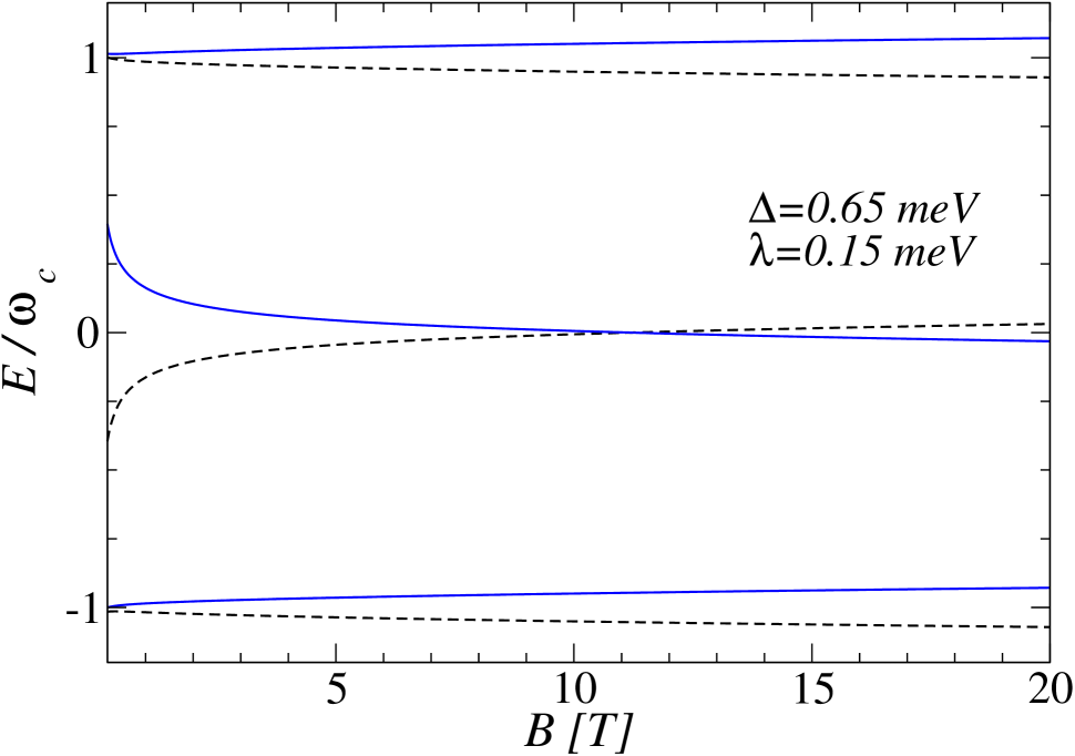
Figure 1: (Color online) Low-lying Landau level energies (in units of the cyclotron energy $\hbar\omega_{c}$) vs magnetic field $B$ (in Tesla) for the SOI parameters $\Delta=0.65$ meV and $\lambda=0.15$ meV. For small $B$, this corresponds to the QSH phase, $\Delta>\lambda/2$. For better visibility, the deviation from the respective $\Delta=\lambda=b=0$ level has been magnified by a factor 10 for each curve.

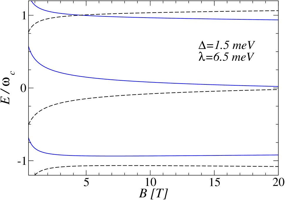
Figure 2: (Color online) Same as in Fig. 1 but for $\Delta=1.5$ meV and $\lambda=6.5$ meV.

III.4 Spin polarization

Given the Landau level eigenstates, it is straightforward to compute the spin-polarization densities $S_{i}(y)=\Psi^{\dagger}\frac{s_{i}}{2}\Psi$ ($i=x,y,z$). We find $S_{x}(y)=0$, while

$$S_{y}(y) = \frac{\nu-p}{\lambda{\cal N}_{p}}\left(pD_{p-1}D_{p}+\frac{\nu_{-}}{\mu_{-}}D_{p}D_{p+1}\right),$$ (66)

$$S_{z}(y) = \frac{1}{2{\cal N}_{p}}\Biggl{[}p^{2}D_{p-1}^{2}+\left(\nu_{-}^{2}-\frac{(\nu-p)^{2}}{\lambda^{2}}\right)D_{p}^{2}$$

$$-\quad\frac{(\nu-p)^{2}}{\lambda^{2}\mu_{-}^{2}}D_{p+1}^{2}\Biggr{]},$$

where $D_{p}\equiv D_{p}(-\eta)$. In the absence of the Rashba term ($\lambda=0)$, the in-plane component $S_{y}$ vanishes identically, since then the eigenstates are simultaneously eigenstates of $s_{z}$. For finite $\lambda$, integration over $y$ yields a vanishing expectation value for the overall in-plane polarization, but the Rashba coupling still induces local in-plane spin polarization. The case $\Delta=b=0$ has been discussed in detail by Rashba.rashba

IV QH edge states for intrinsic SOI

In this section, we consider the edge states corresponding to the relativistic Landau level problem in Sec. III when a boundary at $y=0$ is present. We focus on the case of purely intrinsic SOI, $\lambda=0$, but the physics should be qualitatively unchanged for $\lambda\ll\Delta$. In the region $y<0$ we then have a homogeneous magnetic field $B_{z}=+B$, i.e, $\epsilon=+1$. (For a pseudo-magnetic field, this holds at the $K$ point while at the $K^{\prime}$ point, $B_{z}\to-B_{z}$.)

Since the problem of edge states in graphene has been studied extensively before, some remarks are in order at this point. In fact, putting $\Delta=b=\lambda=0$, our results are consistent with those of Refs. fertig1, ; peres, ; kormanyos1, ; mont, ; landman, reporting chiral QH edge states in graphene. On the other hand, the $B=0$ model is equivalent to the continuum limit of the Kane-Mele modelkane and thus exhibits helical QSH edge states.qsh (The helical state has a pair of counterpropagating 1D modes with opposite spin polarization.) The Kane-Mele model with $(\Delta,b)\neq 0$ but without orbital magnetic field has recently been studied,yang and a quantum phase transition from a (generalized) QSH phase for $b<\Delta$ to a quantum anomalous Hall (QAH) phase for $b>\Delta$ has been predicted. It is worthwhile to stress that the QSH effect survives even when time-reversal symmetry is broken. In the QAH phase, one has chiral edge states moving in the same direction for both spin polarizations.alan The valley analogue of this quantum phase transition has also been studied.niu Furthermore, for the 2D topological insulator realized in HgTe quantum well structures, a related transition has been predictedtkachov by including the orbital field but omitting the Zeeman term.

However, the Zeeman term is crucial in graphene near the Dirac point: for $\Delta=0$ and $b\neq 0$, spin-filtered helical edge states (similar to the QSH case) emerge again.abanin ; arikawa Our results below show that this QSH-like phase is separated from the “true” QSH phase by a quantum phase transition at $b=\Delta$. Albeit both phases have spin-filtered edge states, they differ in the direction of the spin current. This feature should allow to experimentally distinguish both phases and to identify the quantum phase transition separating them. In practice, one may reach this transition simply by changing the magnetic field.

Normalizability of the wavefunctions for $y\to-\infty$ impliesabram that the only allowed solutions follow from the $\phi_{p}$ spinors in Eq. (30), while the $\psi_{p}$ solutions [Eq. (40)] have to be discarded. Since we do not have to impose normalizability at $y\to\infty$, the order $p$ is not constrained to integer values and can now take any real value consistent with suitable boundary conditions at $y=0$. For given conserved momentum $k_{x}$ and spin $s$, the solutions for $p$ yield the edge state spectrum, $E_{s}(k_{x})$. Note that for finite magnetic field and $k_{x}<0$, the distance from the boundary is set by $|k_{x}|$. Putting $\lambda=0$, possible solutions $\phi^{K,K^{\prime}}_{p,\pm,s}(y)$ must be of the form in Eq. (58), with energy $E_{p,\pm,s}$ given by Eq. (62). While $p\in\mathbb{N}_{0}$ in Sec. III.2, we now consider arbitrary real $p$. To make progress, we have to specify boundary conditions at $y=0$. We investigate two widely used boundary conditions, namely the zig-zag edge and the armchair edge.review2 ; abanin ; fertig ; akh

IV.1 Zig-zag edge

For a zig-zag edge with the last row of carbon atoms residing on, say, sublattice $A$, the microscopic wavefunction must vanish on the next row outside the sample, belonging to sublattice $B$. In the continuum limit, since the $x$-axis here points in the zig-zag direction, the lower component of the spinor $\phi^{K}_{p,\pm,s}$ [Eq. (58)] has to vanish at $y=0$.abanin ; fertig1 For both spin directions $s=\pm$, this yields the condition

$$D_{p}(2k_{x})=0,$$ (67)

which has to be solved for the energy, expressed in terms of $p$ as $E_{s}=sb\pm\sqrt{p+\Delta^{2}}$. At the other Dirac point, the lower component of the spinor $\phi^{K^{\prime}}_{p,\pm,s}$ should vanish at $y=0$, where Eq. (21) implies the condition

$$\nu_{p,\pm,s}D_{p-1}(2k_{x})=0,$$ (68)

with $\nu_{p,\pm,s}$ in Eq. (63). It is not possible to find simultaneous solutions to both Eqs. (67) and (68). Possible states are thus confined to a single valley: the boundary condition does not mix the valleys but lifts the $KK^{\prime}$ degeneracy. Remarkably, for $s=\pm$ and arbitrary $k_{x}$, Eq. (68) is satisfied by the $K^{\prime}$ solution for $p=0$ in Sec. III.2, with $E_{s}(k_{x})=s(b-\Delta)$, i.e., we find a pair of “flat” states. For all other states, Eq. (68) simplifies to condition (67) with $p\to p-1$ (and $K\to K^{\prime}$). We mention in passing that for $\Delta=0$ this condition reduces to Eq. (9) in Ref. landman, . Equation (67) can be solved in closed form for $k_{x}\to-\infty$ using asymptotic properties of the parabolic cylinder function. To exponential accuracy, with $n\in\mathbb{N}_{0}$ we find

$$p=n+\frac{|2k_{x}|^{2n+1}}{\sqrt{2\pi}n!}e^{-2k_{x}^{2}}.$$ (69)

Numerical analysis of the above equations recovers the expected spin-filtered helical edge statesabanin for $b>\Delta$, but the continuum approach used in this paper fails to give clear evidence for the helical QSH edge states for $b<\Delta$. As pointed out in Ref. arikawa, , under the zig-zag boundary condition one needs a more microscopic description in order to capture these states. The “flat” states above are remnants of the sought QSH edge states, but the continuum model is not sufficient to describe their proper dispersion relation. We therefore turn to the armchair boundary condition.

IV.2 Armchair edge

Under the armchair boundary condition, we instead impose $\Psi_{A}^{K}+\Psi_{A}^{K^{\prime}}=0$ and $\Psi_{B}^{K}+\Psi_{B}^{K^{\prime}}=0$ at the boundary, with $\Psi$ in Eq. (1). This boundary condition mixes the valleys and involves both sublattices. Since in our coordinate system the $x$-axis is parallel to the zig-zag direction, we first rotate the system by $\pi/2$ and then impose the boundary condition at $y=0$. Written in the original coordinates, we find (for each spin direction $s$)

$$\nu_{p,\pm,s}D_{p-1}(2k_{x})\pm D_{p}(2k_{x})=0.$$ (70)

We note that the relative phase between the $K$ and $K^{\prime}$ components is not fixed by the Dirac equation, which is diagonal in valley space. However, the only relative phase compatible with the boundary condition imposed simultaneously on both sublattices is $\pm 1$. Each of the two conditions in Eq. (70) may thus be imposed separately. We have checked that the numerical solution of Eq. (70) for $\Delta=0$ recovers the known results for the QH edge state spectrum.abanin ; landman In addition, for $B=0$, the armchair edge is known fertig ; sandler to yield QSH edge states.

Our numerical results for the dispersion relation $E_{s,\pm}(k_{x})$ for the armchair edge are shown in Fig. 3, where $\pm$ corresponds to the symmetric or antisymmetric linear combination in Eq. (70) and the magnetic field is $B=15$ T. The main panel shows results for $\Delta=6$ meV. Then $\Delta>b$, and we have the (generalized) QSH phase. Indeed, for $E=0$ we find the helical edge state, where the right- (left-)mover has spin $s=\uparrow$ $(s=\downarrow)$. The inset of Fig. 3 is for $\Delta=0.3$ meV, where $\Delta<b$ and the spin-filtered helical QH phaseabanin is found. Here we have spin $s=\downarrow$ ($s=\uparrow$) for the right- (left-)mover. Hence the spin current differs in sign for $\Delta>b$ and $\Delta<b$, with a quantum phase transition at $\Delta=b$ separating both phases. This feature should allow for an experimentally observable signature of the transition.

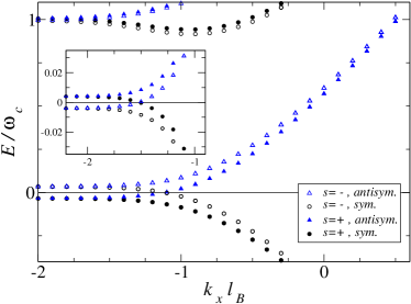
Figure 3: (Color online) Dispersion relation $E_{s,\pm}(k_{x})$ of a semi-infinite graphene sheet with an armchair edge at $y=0$, obtained numerically from Eq. (70). We use $\lambda=0$, $B=15$ T, $\Delta=6$ meV, and the $+$ ($-$) sign is for the symmetric (antisymmetric) valley combination in Eq. (70). Inset: Same for $\Delta=0.3$ meV.

V Spin structure in magnetic waveguides

In this section, a spatially inhomogeneous situation is considered, where a magnetic waveguidelambert ; ghosh ; haus1 along the $x$-direction can be realized. Since the problem remains homogeneous along the $x$-direction, $p_{x}=\hbar k_{x}$ is still conserved. For the physics described below, the Zeeman coupling $b$ gives only tiny correctionshaus1 and will be neglected. Moreover, there are no valley-mixing terms such that we can focus on a single valley.

We distinguish a central strip of width $2L$ (the “waveguide”), $-L<y<L$, and two outer regions $y<-L$ and $y>L$. In the central strip, we shall allow for arbitrary SOI parameters $\Delta$ and $\lambda$. In addition, strain may cause a constant contribution to the vector potential, ${\cal A}_{x}$, and a scalar potential, $V$. The magnetic field in the central strip is denoted by $B_{c}$. For $|y|>L$, we assume that all strain- or SOI-related effects can be neglected, $\Delta=\lambda={\cal A}_{x}=V=0$. In principle, by lithographic deposition of adatoms, one may realize this configuration experimentally. For $y<-L$, the magnetic field is $B_{z}=B>0$, while for $y>L$, we set $B_{z}=\epsilon B$, where $\epsilon=1$ ($\epsilon=-1$) corresponds to the parallel (antiparallel) field orientation on both sides. For $\epsilon=-1$, we take $B_{c}=0$, while for $\epsilon=+1$, we set $B_{c}=-B$.

The setup with $\epsilon=-1$ could be realized by using a “folded” geometry,folded ; rainis cf. recent experimental studies.fold2 Note that when the magnetic field changes sign, one encounters “snake orbits,” which have been experimentally observed in graphene $pn$ junctions.snake For the $\epsilon=-1$ configuration, we have uni-directional snake orbits mainly localized along the waveguide, while for $\epsilon=+1$, we get two counterpropagating snake states centered near $y=\pm L$. For $\Delta=\lambda={\cal A}_{x}=V=0$, both cases ($\epsilon=\pm 1$) have been studied in detail in Ref. ghosh, . Technically, one determines the eigenstates and the spectrum, $E(k_{x})$, by matching the wavefunctions in the three different regions, which results in an energy quantization condition. This method can be straightforwardly extended to the more complex situation studied here by employing the general solution in Sec. II for the central strip.

Before turning to results, we briefly summarize the parameter values chosen in numerical calculations. We take a magnetic field value $B=0.2$ T, and the waveguide width is $2L=\sqrt{8}\ell_{B}\approx 40$ nm. The strain-induced parameters in the central strip are taken as ${\cal A}_{x}=-16\mu$m^-1 and $V=-20$ meV. These values have been estimated for a folded setup,rainis where $V$ comes from the deformation potential. We consider two different parameter choices for the SOI couplings: Set (A) has $\Delta=13$ meV and $\lambda=3$ meV, corresponding to the QSH phase. For set (B), we exchange both values, i.e., $\Delta=3$ meV and $\lambda=13$ meV.

V.1 Antiparallel case: Snake orbit

Let us first discuss the $\epsilon=-1$ configuration, where the magnetic field $B_{z}$ differs in sign in the regions $y<-L$ and $y>L$. The dispersion relation of typical low-energy 1D waveguide modes is shown in Fig. 4. For $k_{x}\to-\infty$ the centers of the quantum states are located deep in the left and right magnetic regions, far from the waveguide. Thus one has doubly-degenerate dispersionless “bulk” Landau states. With increasing $k_{x}$ these states are seen to split up. The dominant splitting, which is already present for $\Delta=\lambda=0$, comes from the splitting of symmetric and anti-symmetric linear combinations of the Landau states for $y<-L$ and $y>L$ with increasing overlap in the waveguide region.ghosh Asymptotically, the dispersion relation of all positive-energy snake states is $E(k_{x}\to+\infty)\simeq\hbar v_{F}k_{x}$.ghosh For intermediate $k_{x}$ and $(\Delta,\lambda)\neq 0$, however, we get spin-split snake states out of the previously spin-degenerate states. The spin splitting is mainly caused by the Rashba coupling $\lambda$ and disappears for $\lambda\to 0$, cf. the inset of Fig. 4.

The zero-energy bulk Landau state (for $k_{x}\to-\infty$) shows rich and interesting behavior in this setup. While for $k_{x}\to+\infty$, we expect one pair of snake states with positive slope and one pair with negative slope, for the studied parameter set and range of $k_{x}L$, there is just one state with negative slope while three branches first move down and then have a positive slope. Accordingly, at the Dirac point ($E=0$), Fig. 4 shows that there are three right-movers with different Fermi momenta and different spin texture. Two of those states are indicated by stars (*) in the main panel of Fig. 4 and their local spin texture is shown in Fig. 5. Evidently, they are mainly localized inside the waveguide and have antiparallel spin polarization. We find spin densities with $S_{x}=0$ for both states. For the Rashba-dominated situation in Fig. 5, spin is polarized perpendicular to the current direction and has a rather complex spatial profile.

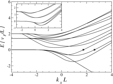
Figure 4: Dispersion relation of the lowest few energy branches for a strained magnetic waveguide with $\epsilon=-1$ and SOI in the central strip of width $2L$. Energies are given in units of $\hbar v_{F}/L$. The main panel is for parameter set (B). The stars refer to the states further studied in Fig. 5. Inset: Same for set (A). (See main text for details.)

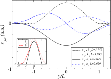
Figure 5: (Color online) Spin density profile $S_{y,z}$ (in arbitrary units) vs $y/L$ for the two $E=0$ right-moving states indicated by stars in the main panel of Fig. 4. The left star corresponds to $k_{x}L=1.745$, the right star to $k_{x}L=2.629$. Inset: Particle density, $\rho$, and current density, $J_{x}$ (which is the only non-vanishing component), in arbitrary units vs $y/L$. We show the result only for $k_{x}L=1.745$, since $k_{x}L=2.629$ yields practically the same.

V.2 Parallel configuration

Next we come to the $\epsilon=+1$ configuration, where the magnetic field is $+B$ for $|y|>L$ and $-B$ for $|y|<L$. One therefore expects two counterpropagating snake states in the $x$-direction localized around $y=\pm L$. The corresponding spectrum is shown in Fig. 6. We focus on parameter set (B), since for set (A), the spin splitting is minimal and less interesting. The spectrum consists of two qualitatively different states, namely states of bulk Landau character for large $|k_{x}|L$, and a set of propagating waveguide modes.ghosh The spectral asymmetry seen in Fig. 6 for all propagating modes, $E(-k_{x})\neq E(k_{x})$, is caused by the strain (${\cal A}_{x}$)-induced shift of $k_{x}$. Such a spectral asymmetry may give rise to interesting chirality and magnetoasymmetry effects.tsvelik The spin texture is shown in Fig. 7 for a pair of right- and left-moving states with $E=1.2\hbar v_{F}/L$, cf. the stars in Fig. 6. We observe from the main panel in Fig. 7 that the spin polarization of both states is approximately antiparallel. Because of their spatial separation and the opposite spin direction, elastic disorder backscattering between these counterpropagating snake modes should be very strongly suppressed. The inset of Fig. 7 shows the current density profile across the waveguide. Although the profile is quite complex, we observe that the current has opposite sign for both modes.

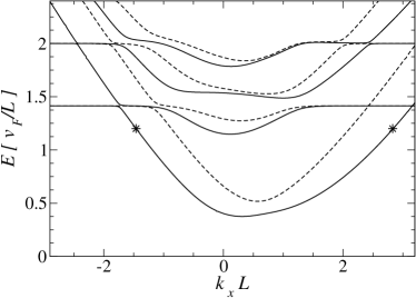
Figure 6: Same as Fig. 4 but for the setup with $\epsilon=+1$ and parameter set (B). Solid and dashed curves are for better visibility only. The two states indicated by stars are studied in Fig. 7.

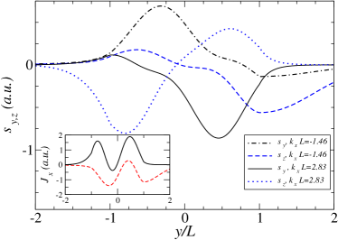
Figure 7: (Color online) Spin density $S_{y,z}$ (in arbitrary units) vs $y/L$ for the two states indicated by stars in Fig. 6. The left (right) star corresponds to a left- (right-)mover with $k_{x}L=-1.46$ ($k_{x}L=2.83$). Note that the spin polarizations of both states are approximately antiparallel. Inset: Particle current profile $J_{x}$ (in arbitrary units) vs $y/L$ for both states. Black solid curve: $k_{x}L=2.83$. Dashed red curve: $k_{x}L=-1.46$.

VI Concluding remarks

In this work, we have studied the magnetoelectronic properties of monolayer graphene in the presence of strong intrinsic and Rashba-type spin-orbit couplings. According to a recent proposal,franz large intrinsic couplings may be realized by suitable adatom deposition on graphene. We have presented an exact solution for the Landau level states for arbitrary SOI parameters. When the intrinsic SOI dominates, by increasing the magnetic field, we predict a quantum phase transition from the quantum spin Hall phase to a helical quantum Hall phase at the Dirac point. In both phases, one has spin-filtered edge states but with opposite spin current direction. Thus the transition could be detected by measuring the spin current either in a transport experiment (e.g., along the lines of Ref. tombros, ) or via a magneto-optical experiment.

In inhomogeneous magnetic fields, especially when also strain-induced pseudo-magnetic fields are present, interesting waveguides can be envisioned. Such setups allow for snake states, where spin-orbit couplings result in a spin splitting. In a double-snake setup, there is a pair of counterpropagating snake states that carry (approximately) opposite spin polarization. This implies that scattering by elastic impurities is drastically suppressed. The resulting spin textures can in principle be detected by spin resolved ARPES (see, e.g., Refs. dedkov, and bostwick, ) or spin-polarized STM measurements.

We hope that our predictions can soon be tested experimentally.

Appendix A Derivation of the eigenstates

Here we provide some details concerning the derivation of Eq. (30); the notation below is explained in Sec. II. First, additional relations like Eq. (23) can be stated,

$$aD_{p}(-\eta) = -pD_{p-1}(-\eta),\quad a^{\dagger}D_{p}(-\eta)=-D_{p+1}(-\eta),$$

$$aD_{p}(i\eta) = -iD_{p+1}(i\eta),\quad a^{\dagger}D_{p}(i\eta)=-ipD_{p-1}(i\eta).$$

We wish to construct the solution $\phi=(\phi_{1},\phi_{2},\phi_{3},\phi_{4})^{T}$ satisfying Eq. (22),

$$\left(\begin{array}[]{cccc}\nu_{-}&a&0&0\\ a^{\dagger}&\nu_{+}&i\lambda&0\\ 0&-i\lambda&\mu_{+}&a\\ 0&0&a^{\dagger}&\mu_{-}\end{array}\right)\left(\begin{array}[]{c}\phi_{1}\\ \phi_{2}\\ \phi_{3}\\ \phi_{4}\end{array}\right)=0.$$

We here show only the case $\epsilon=+1$ near the $K$ point; all other cases follow analogously. Solving the first and last equations for $\phi_{1}$ and $\phi_{4}$, respectively, we find

$$\phi_{1}=-\frac{1}{\nu_{-}}a\phi_{2},\quad\phi_{4}=-\frac{1}{\mu_{-}}a^{\dagger}\phi_{3}.$$

For $\mu_{-}=0$, one has the solution (48) instead, while for $\nu_{-}=0$ there are no solutions. The second and third equations then yield two coupled second-order ordinary differential equations for $\phi_{2}$ and $\phi_{3}$,

$$(a^{\dagger}a-\nu)\phi_{2}-i\lambda\nu_{-}\phi_{3} = 0,$$

$$i\lambda\mu_{-}\phi_{2}+(a^{\dagger}a+1-\mu)\phi_{3} = 0.$$

Solving for $\phi_{3}$ yields

$$\phi_{3}=\frac{1}{i\lambda\nu_{-}}(a^{\dagger}a-\nu)\phi_{2},$$

and we thus arrive at the equation

$${\cal D}\phi_{2}\equiv\left[(a^{\dagger}a+1-\mu)(a^{\dagger}a-\nu)-\lambda\mu_{-}\nu_{-}\right]\phi_{2}=0.$$

Since the operator ${\cal D}$ commutes with the “number operator” $a^{\dagger}a$, the sought solutions for $\phi_{2}$ span the kernel of ${\cal D}$ where the $\phi_{2}$ are eigenstates of $a^{\dagger}a$,

$$a^{\dagger}a\ \phi_{2,p}(\eta)=p\ \phi_{2,p}(\eta).$$

This leads to an algebraic equation for the eigenvalue $p$,

$$(p+1-\mu)(p-\nu)=\lambda^{2}\mu_{-}\nu_{-},$$

which implies the two solutions in Eq. (24). With $a^{\dagger}a=(\eta/2)^{2}-1/2-d^{2}/d\eta^{2}$, the eigenvalue equation for $\phi_{2}$ is just the differential equation of the parabolic cylinder functions,abram

$$\left(\frac{d^{2}}{d\eta^{2}}+p+\frac{1}{2}-\frac{\eta^{2}}{4}\right)\phi_{2}(\eta)=0,$$

which has the four (linearly dependent) solutions $\{D_{p}(\eta),D_{p}(-\eta),D_{-p-1}(i\eta),D_{-p-1}(-i\eta)\}$. Given the solution for $\phi_{2}$, all other components in $\phi$ follow by using the recurrence relations of the $D_{p}$ functions, see, e.g., Eq. (23). After straightforward but lengthy algebra, we obtain the four solutions (also quoted for $\epsilon=-1$)

$$\phi_{\epsilon=+1,p} = \left(\begin{array}[]{c}-pD_{p-1}(\eta)\\ \nu_{-}D_{p}(\eta)\\ \frac{i(\nu-p)}{\lambda}D_{p}(\eta)\\ \frac{-i(\nu-p)}{\lambda\mu_{-}}D_{p+1}(\eta)\end{array}\right),\quad\left(\begin{array}[]{c}pD_{p-1}(-\eta)\\ \nu_{-}D_{p}(-\eta)\\ \frac{i(\nu-p)}{\lambda}D_{p}(-\eta)\\ \frac{i(\nu-p)}{\lambda\mu_{-}}D_{p+1}(-\eta)\end{array}\right),$$

$$\psi_{\epsilon=+1,p} = \left(\begin{array}[]{c}-iD_{-p}(-i\eta)\\ \nu_{-}D_{-p-1}(-i\eta)\\ \frac{i(\nu-p)}{\lambda}D_{-p-1}(-i\eta)\\ \frac{-(\nu-p)(p+1)}{\lambda\mu_{-}}D_{-p-2}(-i\eta)\end{array}\right),\quad\left(\begin{array}[]{c}-iD_{-p}(i\eta)\\ \nu_{-}D_{-p-1}(i\eta)\\ \frac{i(\nu-p)}{\lambda}D_{-p-1}(i\eta)\\ \frac{(\nu-p)(p+1)}{\lambda\mu_{-}}D_{-p-2}(i\eta)\end{array}\right),$$

$$\phi_{\epsilon=-1,p} = \left(\begin{array}[]{c}-D_{p+1}(-\eta)\\ \mu_{-}D_{p}(-\eta)\\ \frac{i(\mu-p-1)}{\lambda}D_{p}(-\eta)\\ \frac{-i(\mu-p-1)}{\lambda\nu_{-}}D_{p-1}(\eta)\end{array}\right),\quad\left(\begin{array}[]{c}D_{p+1}(\eta)\\ \mu_{-}D_{p}(\eta)\\ \frac{i(\mu-p-1)}{\lambda}D_{p}(\eta)\\ \frac{i(\mu-p-1)}{\lambda\nu_{-}}D_{p-1}(\eta)\end{array}\right),$$

$$\psi_{\epsilon=-1,p} = \left(\begin{array}[]{c}-i(p+1)D_{-p}(-i\eta)\\ \mu_{-}D_{-p-1}(-i\eta)\\ \frac{i(\mu-p-1)}{\lambda}D_{-p-1}(-i\eta)\\ \frac{(\mu-p-1)}{\lambda\nu_{-}}D_{-p-2}(-i\eta)\end{array}\right),\quad\left(\begin{array}[]{c}i(p+1)D_{-p}(i\eta)\\ \mu_{-}D_{-p-1}(i\eta)\\ \frac{i(\mu-p-1)}{\lambda}D_{-p-1}(i\eta)\\ -\frac{(\mu-p-1)}{\lambda\nu_{-}}D_{-p-2}(i\eta)\end{array}\right).$$

For a given energy $E$, Eq. (22) admits precisely four linearly independent solutions for $\phi$. However, Eq. (24) implies two possible values for $p$, i.e., we have the freedom to choose just two out of the four quoted eigenstates (for given $\epsilon$) and then allow both values of $p$ in Eq. (24). Our conventions for these two basis states are specified in Eqs. (30) and (40) in the main text. Thereby we have obtained all possible solutions to Eq. (22).

References

- (1) A.K. Geim, Science 324, 1530 (2009).
- (2) C.W.J. Beenakker, Rev. Mod. Phys. 80, 1337 (2008).
- (3) A.H. Castro Neto, F. Guinea, N.M.R. Peres, K.S. Novoselov, and A. Geim, Rev. Mod. Phys. 81, 109 (2009).
- (4) C.L. Kane and E.J. Mele, Phys. Rev. Lett. 95, 226801 (2005).
- (5) M.Z. Hasan and C.L. Kane, Rev. Mod. Phys. 82, 3045 (2010).
- (6) M. König, H. Buhmann, L.W. Molenkamp, T. Hughes, C.X. Liu, X.L. Qi, and S.C. Zhang, J. Phys. Soc. Jpn. 77, 031007 (2008).
- (7) D. Huertas-Hernando, F. Guinea, and A. Brataas, Phys. Rev. B 74, 155426 (2006).
- (8) H. Min, J.E. Hill, N.A. Sinitsyn, B.R. Sahu, L. Kleinman, and A.H. MacDonald, Phys. Rev. B 74, 165310 (2006).
- (9) Y. Yao, F. Ye, X.L. Qi, S.C. Zhang, and Z. Fang, Phys. Rev. B 75, 041401(R) (2007).
- (10) Yu.S. Dedkov, M. Fonin, U. Rüdiger, and C. Laubschat, Phys. Rev. Lett. 100, 107602 (2008).
- (11) A. Varykhalov, J. Sánchez-Barriga, A.M. Shikin, C. Biswas, E. Vescovo, A. Rybkin, D. Marchenko, and O. Rader, Phys. Rev. Lett. 101, 157601 (2008).
- (12) C. Weeks, J. Hu, J. Alicea, M. Franz, and R. Wu, preprint arXiv:1104.3282.
- (13) M.A.H. Vozmediano, M.I. Katsnelson, and F. Guinea, Phys. Rep. 496, 109 (2010).
- (14) A.H. Castro Neto and F. Guinea, Phys. Rev. Lett. 103, 026804 (2009).
- (15) D. Huertas-Hernando, F. Guinea, and A. Brataas, Phys. Rev. Lett. 103, 146801 (2009).
- (16) E.I. Rashba, Phys. Rev. B 79, 161409(R) (2009).
- (17) D. Bercioux and A. De Martino, Phys. Rev. B 81, 165410 (2010).
- (18) L. Lenz and D. Bercioux, arXiv:1106.4242.
- (19) F. Guinea, M.I. Katsnelson, and A.K. Geim, Nat. Phys. 6, 30 (2010).
- (20) D.A. Abanin, P.A. Lee, and L.S. Levitov, Phys. Rev. Lett. 96, 176803 (2006); D.A. Abanin, P.A. Lee, and L.S. Levitov, Sol. St. Comm. 143, 77 (2007).
- (21) V.P. Gusynin and S.G. Sharapov, Phys. Rev. Lett. 95, 146801 (2005).
- (22) L. Brey and H.A. Fertig, Phys. Rev. B 73, 195408 (2006).
- (23) N.M.R. Peres, A.H. Castro Neto, and F. Guinea, Phys. Rev. B 73, 241403 (2006).
- (24) A. De Martino, L. Dell’Anna, and R. Egger, Phys. Rev. Lett. 98, 066802 (2007).
- (25) M. Ramezani Masir, P. Vasilopoulos, A. Matulis, and F.M. Peeters, Phys. Rev. B 77, 235443 (2008).
- (26) L. Oroszlány, P.K. Rakyta, A. Kormányos, C.J. Lambert, and J. Cserti, Phys. Rev. B 77, 081403(R) (2008).
- (27) T.K. Ghosh, A. De Martino, W. Häusler, L. Dell’Anna, and R. Egger, Phys. Rev. B 77, 081404(R) (2008).
- (28) W. Häusler, A. De Martino, T.K. Ghosh, and R. Egger, Phys. Rev. B 78, 165402 (2008).
- (29) L. Dell’Anna and A. De Martino, Phys. Rev. B 79, 045420 (2009).
- (30) L. Dell’Anna and A. De Martino, Phys. Rev. B 80, 155416 (2009).
- (31) A. De Martino and R. Egger, Semicond. Sci. Techn. 25, 034006 (2010).
- (32) R. Egger, A. De Martino, H. Siedentop, and E. Stockmeyer, J. Phys. A 43, 215202 (2010).
- (33) L. Dell’Anna and A. De Martino, Phys. Rev. B 83, 155449 (2011).
- (34) L.D. Landau and E.M. Lifshitz, Elasticity Theory (Pergamon, New York, 1986).
- (35) H. Suzuura and T. Ando, Phys. Rev. B 65, 235412 (2002).
- (36) M.M. Fogler, F. Guinea, and M.I. Katsnelson, Phys. Rev. Lett. 101, 226804 (2008).
- (37) A different representation for has been given in Ref. beenakker, because of a different arrangement of the sublattice components in the spinor [Eq. (1)].
- (38) M. Abramowitz and I.A. Stegun, Handbook of Mathematical Functions, ch. 19 (Dover, New York, 1965).
- (39) I.S. Gradshteyn and I.M. Ryzhik, Table of Integrals, Series, and Product (Academic Press, Inc., New York, 1980).
- (40) For notational convenience, we shift for in the discussion of the purely intrinsic SOI.
- (41) We note that we made a wrong statement in Ref. ssc, in that direction: For the case on page 3 therein, we stated that for there are two normalizable states with which for coalesce into a single zero-energy Landau level. However, only the state is allowed, and the other one is not normalizable.
- (42) P. Rakyta, A. Kormányos, J. Cserti, and P. Koskinen, Phys. Rev. B 81, 115411 (2010).
- (43) P. Delplace and G. Montambaux, Phys. Rev. B 82, 205412 (2010).
- (44) I. Romanovsky, C. Yannouleas, and U. Landman, Phys. Rev. B 83, 045421 (2011).
- (45) Y. Yang, Z. Xu, L. Sheng, B. Wang, D.Y. Xing, and D.N. Sheng, Phys. Rev. Lett. 107, 066602 (2011).
- (46) Z. Qiao, S.A. Yang, W. Feng, W.K. Tse, J. Ding, Y. Yao, J. Wang, and Q. Niu, Phys. Rev. B 82, 161414(R) (2010); W.K. Tse, Z. Qiao, Y. Yao, A.H. MacDonald, and Q. Niu, Phys. Rev. B 83, 155447 (2011).
- (47) W. Yao, S.A. Yang, and Q. Niu, Phys. Rev. Lett. 102, 096801 (2009).
- (48) G. Tkachov and E.M. Hankiewicz, Phys. Rev. Lett. 104, 166803 (2010); Phys. Rev. B 83, 155412 (2011).
- (49) M. Arikawa, Y. Hatsugai, and H. Aoki, Phys. Rev. B 78, 205401 (2008).
- (50) K. Nakada, M. Fujita, G. Dresselhaus, and M.S. Dresselhaus, Phys. Rev. B 54, 17954 (1996); L. Brey and H.A. Fertig, Phys. Rev. B 73, 235411 (2006).
- (51) A.R. Akhmerov and C.W.J. Beenakker, Phys. Rev. B 77, 085423 (2008).
- (52) J. Tworzydlo, B. Trauzettel, M. Titov, A. Rycerz, and C.W.J. Beenakker, Phys. Rev. Lett. 96, 246802 (2006); M. Zarea and N. Sandler, Phys. Rev. Lett. 99, 256804 (2007).
- (53) E. Prada, P. San-Jose, and L. Brey, Phys. Rev. Lett. 105, 106802 (2010).
- (54) D. Rainis, F. Taddei, M. Polini, G. León, F. Guinea, and V.I. Fal’ko, Phys. Rev. B 83, 165403 (2011).
- (55) K. Kim, Z. Lee, B.D. Malone, K.T. Chan, B. Alemán, W. Regan, W. Gannett, M.F. Crommie, M.L. Cohen, and A. Zettl, Phys. Rev. B 83, 245433 (2011).
- (56) J.R. Williams and C.M. Marcus, Phys. Rev. Lett. 107, 046602 (2011).
- (57) A. De Martino, R. Egger, and A.M. Tsvelik, Phys. Rev. Lett. 97, 076402 (2006).
- (58) N. Tombros, C. Josza, M. Popinciuc, H.T. Jonkman, and B.J. van Wees, Nature 448, 571 (2007).
- (59) A. Bostwick et al., Science 328, 999 (2010).