Superfluid density and phase relaxation in superconductors with strong disorder

Abstract

As a prototype of a disordered superconductor we consider the attractive Hubbard model with on-site disorder. We solve the Bogoljubov-de-Gennes equations on two-dimensional finite clusters at zero temperature and evaluate the electromagnetic response to a vector potential. We find that the standard decoupling between transverse and longitudinal response does not apply in the presence of disorder. Moreover the superfluid density is strongly reduced by the relaxation of the phase of the order parameter already at mean-field level when disorder is large. We also find that the anharmonicity of the phase fluctuations is strongly enhanced by disorder. Beyond mean-field, this provides an enhancement of quantum fluctuations inducing a zero-temperature transition to a non-superconducting phase of disordered preformed pairs. Finally, the connection of our findings with the glassy physics for extreme dirty superconductors is discussed.

In the last few years renewed interest emerged in the behavior of disordered superconductors at the verge of the metal-insulator transition. On the experimental side recent studies of disordered superconducting films at low-temperatures sacepe09 ; mondal10 have revealed the existence of a striking “pseudogap” behavior at large disorder, with the tunneling conductance at zero bias starting to develop a suppression at temperatures much larger than $T_{c}$. These findings suggest quite generically a separation between the energy scales associated to local pairing (gap and pseudogap) and superconducting phase coherence (superfluid density) with different dependencies on disorder. In particular, it is this second energy scale (to be more specific, the superfluid stiffness) which is expected to control the stability of the superconducting phase in the proximity to the superconductor-insulator (SC-I) transition.

From the theoretical point of view the study of disordered superconductors near the SC-I transitionfeigelman10 has been based either on a bosonic approachfisher90 , where the role of phase fluctuations emerges naturally, or on a more microscopic fermionic approachranderia01 ; feigelman07 ; dubi07 ; randeria10 , which has put the focus on the emergence of a short-scale inhomogeneity induced by the strong disorder. In particular, in the latter case the appearance of two characteristics features of the disordered SC state has been demonstrated: the spontaneous emergence of spatial structures in the local pairing gap and a general suppression of the phase coherence, which reflects in a decrease of the global superfluid stiffnessranderia01 ; dubi07 ; feigelman07 ; randeria10 . These results appear already at mean-field level, as it has been shown by the Bogoljubov-de-Gennes (BdG) solution for a 2D SC system in the presence of on-site disorderranderia01 , which serves also as comparison for more refined Monte Carlo results including thermaldubi07 or quantumranderia10 phase fluctuations. Recently it has been argued that eventually a non self-averaging character typical of glassy physics will appear at very strong disorderIMFIM .

In the presence of disorder a non-trivial problem is posed by the correct computation of the superfluid stiffness $D_{s}$ and by the understanding of the processes leading to the supression of $D_{s}$. In the clean translational invariant case the superfluid behavior of the system reflects the “rigidity” of the phase against an applied transverse vector potential. This leads to a purely diamagnetic response of the current, which is the hallmark of the Meissner effect and the superfluid behavior of clean superconductors. At small disorder a paramagnetic response appears and the superfluid stiffness decreases with respect to the pure diamagnetic case. This paramagnetic current is the response of BdG quasiparticles to the external vector potential, while keeping the phase of the order parameter unchanged. Within the BdG approach, one can then account for this effect by evaluating $D_{s}$ as a disorder average over the BCS response function (the BCS current-current correlation function with no vertex corrections), computed with the BdG solution for the disordered system (cf. e.g. Ref. randeria01 ). This procedure, which for small disorder is equivalent to the dirty-BCS limit, relies on the decoupling between longitudinal and transverse electromagnetic response: the phase of the order parameter does (does not) react to a longitudinal (transverse) field. However, this decoupling holds exactly only in clean systems. Our main results in this work are: i) For strong disorder we show that such a decoupling is strongly violated, leading to a dramatic decrease of the phase stiffness with respect to the dirty BCS case, due to the additional paramagnetic suppression coming from the phase relaxation to the applied transverse vector potential. ii) We discuss the behavior of this paramagnetic phase response in connection to the formation of self-organized structures of the current in real space at scales much larger than the lattice spacing and the SC coherence length [cf. Fig. 1(b)], which share some analogies with the glassy features discussed in Refs. IMFIM . iii) We show that the anharmonic phase fluctuations become strongly enhanced already at intermediate disorder with respect to the clean case, leading to a sizeable increase of quantum corrections to the superfluid stiffness due to phase fluctuations, with respect to a clean system. These results can account for the recently observed deviation of the superfluid stiffness from the dirty-BCS limit in NbN filmsmondal10 , and offer new insight for the understanding of the SC-I transition.

Our starting hamiltonian is the attractive Hubbard model with local disorder:

$$H=-t\sum_{\langle ij\rangle\sigma}c^{\dagger}_{i\sigma}c_{j\sigma}+h.c.-|U|\sum_{i}n_{i\uparrow}n_{i\downarrow}+\sum_{i\sigma}V_{i}n_{i\sigma},$$ (1)

which we solve using the BdG equations degennes by allowing for a site dependent SC order parameter $\Delta_{i}=|U|\langle c_{i\downarrow}c_{i\uparrow}\rangle$. The first sum is over nearest-neighbors pairs and we work on a $L\times L$ system using units such that lattice spacing and $\hbar=c=e=1$. The local potential $V_{i}$ is randomly distributed between $-V_{0}\leq V_{i}\leq V_{0}$. We present results for density $n=0.875$ and at large SC coupling ($U/t=-5$), where the phase-relaxation effects and the connection to the glassy physics become more evident. Similar results are found in a wide parameter range.

The superfluid stiffness $D_{s}$ in the $a=x,y$ direction (corresponding in the continuum limit to $D_{s}=n_{s}/m$ with $n_{s}$ being the superfluid density) is defined as the static limit of the transverse part, $K_{T}$, of the electromagnetic kernel, $K_{ab}$, which describes the current response, $j_{a}=K_{ab}A_{b}$, to an applied electromagnetic field $A_{b}$ (summation over repeated indices is implicit)schrieffer ; scalapino93 .

In principle, the correct evaluation of the superfluid stiffness requires the knowledge of the electromagnetic kernel $K_{ab}$ within a so-called conserving approximation, i.e. an approximation that respects the gauge invariance of the theory. As it is well know, the BCS approximation for $K^{BCS}_{ab}$ is not conserving since, by neglecting the vertex corrections, it does not include the contribution of the phase relaxation to the current-current correlation function schrieffer ; scalapino93 . This is not a problem in the clean case as far as the transverse response is concerned, since phase fluctuations contribute only to the longitudinal part of $K_{ab}$schrieffer . It is easy to check that this no longer holds in the presence of disorder. Indeed, upon considering also the non-local character of the BCS kernel for a disordered system, the effective action for phase fluctuationsbenfatto01 can in general be written at Gaussian level as:

$$S_{g}=\frac{1}{8}\int d^{2}{\bf r}d^{2}{\bf r}^{\prime}(\nabla\theta_{\bf r}-2{\bf A}_{\bf r})_{a}K^{BCS}_{ab}({\bf r},{\bf r}^{\prime})(\nabla\theta_{{\bf r}^{\prime}}-2{\bf A}_{{\bf r}^{\prime}})_{b}.$$ (2)

In the absence of disorder the above expression simplifies considerably, since the BCS kernel $K^{BCS}_{ab}$ depends only on the difference ${\bf r}-{\bf r}^{\prime}$, so that by making the Fourier transform and approximating the BCS kernel with its (constant) long-wavelenght limit $K^{BCS}_{0}\equiv K^{BCS}_{aa}(0)$, the action reduces to:

$$S_{g}=\frac{1}{8}\int d^{2}{\bf r}K^{BCS}_{0}(\nabla\theta-2{\bf A})^{2}.$$ (3)

Integrating by parts the term $\nabla\theta\cdot{\bf A}$, one finds that $\theta$ couples only with the longitudinal part of the electromagnetic field. Integrating out the phase one finds $D_{s}=K_{T}=K^{BCS}_{0}$ i.e. the stiffness is given by the BCS kernel. Modeling disorder by a position dependent kernel in Eq. (3) one sees that the integration by parts leads to a coupling of the phase with both the longitudinal and the transverse part of the gauge field. The same is true if Eq. (2) is used which now depends separately on ${\bf r}$ and ${\bf r}^{\prime}$. For strong disorder one is not allowed to substitute the BCS kernel in Eq. (2) with its space-disordered average which will restore translational invariance and erroneously lead to the simplified Eq. (3). The consequences of this transverse-longitudinal decoupling breakdown are: (i) a change in the SC order-parameter phase even in the presence of a transverse field, contrary to the clean case; (ii) a failure of the BCS response function to compute the superfluid stiffness.

In order to put these arguments on a quantitative basis we first show explicitly the behavior of the current in the presence of a constant vector potential $A$ in the $x$ direction. Using the Peierls substitution, this corresponds to a change in the hopping term of Eq. (1) along $x$:

$$T_{x}(A)=-t\sum_{i\sigma}\left[e^{-iA}c_{i+x,\sigma}^{\dagger}c_{i\sigma}+h.c.\right].$$ (4)

In a torus geometry (periodic boundary conditions) a constant $A$ cannot be gauged away, and it corresponds to a flux $\Phi=AL$ through the torus. For a given disorder configuration the microscopic current along $x$ at finite $A$ is then the sum of the paramagnetic and diamagnetic contribution $j_{x}=-\frac{\partial T_{x}(A)}{\partial(A)}=\langle j_{x}^{P}\rangle+\langle j_{x}^{D}\rangle$. In the clean case $j_{x}$ can be directly derived from Eq. (3), and is proportional to the gauge-invariant phase gradient $\nabla\tilde{\theta}\equiv\nabla\theta-2{\bf A}$. Here $\tilde{\theta}$ is the phase of the order parameter if we would eliminate ${\bf A}$ by a gauge transformation. Since for an applied transverse field $\nabla\theta=0$, then $j_{x}$ reduces to the constant value $-AD_{s}$.

For the disordered system the result is radically different. If one neglects phase relaxation (BCS), each piece of the system responds according to its local stiffness, which is essentially determined by the local order parameter [Fig. 1(a)]. Because this solution is not a saddle point, the current violates charge conservation and is clearly unphysical. Allowing for the phase to relax [Fig. 1(b)] both the current and the gauge invariant phase gradient [proportional to the line density in Fig. 1(a)] are strongly space dependent. This dependence is still correlated to the order parameter but now it is also conditioned by the existence of a percolative path. This means that the current response at one point can be strongly influenced by the local stiffness at very far points. Notice that isolated regions with a robust order parameter have practically zero current in panel (b).

The gauge-invariant phase gradient $\nabla\tilde{\theta}$ is large predominantly in regions with minimum values of the order parameter $\Delta_{i}$. This can be understood by mapping the problem to a random resistor networkpar98 ; kir73 where the bad SC regions map into poor conducting regions and $\tilde{\theta}$ maps into the electrostatic potential, so large “potential” drops concentrate in the “poor” conducting regions. Moreover, in contrast to the clean isotropic case, where $j_{x}$ has the same direction than the gauge-invariant $\nabla\tilde{\theta}$ (see Eq. (3)), here one expects a tensorial relation between the two, as given in Eq. (2) and confirmed by the results of Fig. 1. It is worth stressing that while the local SC order parameter can be quite small, the local density of states always shows a sizable gap, as found in various previous analysesranderia01 ; randeria10 , supporting the view that coherent superconductivity takes place in Fig. 1 on a system of localized preformed pairs.

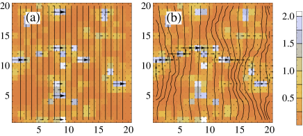
Figure 1: (Color online) Distribution of the local current (arrows) and lines of constant $\tilde{\theta}$ superimposed to the map of the order parameter, neglecting phase relaxation (a) and allowing for it (b). We applied a transverse field $A=0.003$, for a disorder amplitude $V_{0}/t$=2. Notice that in (b), while the percolative pattern of the current goes along the pattern of largest $\Delta_{i}$ values, the gauge-invariant phase gradient is larger along the locations of smaller $\Delta_{i}$ values.

A direct procedure to compute the superfluid stiffness beyond BCS that accounts for the SC-phase relaxation, like those shown in Fig. 1, is given by the change in the ground-state energy $E$ in the presence of the constant vector potential of Eq. (4),khon ; scalapino93

$${D_{s}}=\frac{1}{L^{2}}\frac{\partial^{2}E(A)}{\partial A^{2}}.$$ (5)

The resulting values of $D_{s}$ are shown in Fig. 2, along with their BCS counterparts. While the effects seem not dramatic at the scale of the bare stiffness they are gigantic when the stiffness is small due to strong disorder, as can be seen in the right inset. Such a dramatic difference is clearly due to the global reorganization of the current, i.e. only good SC regions that are along the percolative path contributes to the stiffness. In the BCS case instead the global stiffness results to be a simple spatial average of the local stiffness.

As the stiffness decreses due to increasing disorder also quantum phase fluctuations beyond Gaussian level become relevantranderia01 ; benfatto01 . In general, in the presence of a constant gauge field $A$ the expansion of the energy per unit surface, up to fourth order can be written as:

$$\frac{E}{L^{2}}=\frac{D_{s}}{2}A^{2}-\frac{Qa^{2}}{6}A^{4}=\frac{J}{2}(\delta\theta)^{2}-\frac{J^{\prime}}{24}\xi_{0}^{2}(\delta\theta)^{4}$$ (6)

where $\delta\theta$ is the phase gradient in a given ($x$ or $y$) direction and we have restored explicitly the lattice spacing $a$. From Eq. (6) it is evident that while $D_{s}$ provides the stiffness the coupling $Q$ measures the anharmonicity of the phase fluctuations. The second part of Eq. (6) translates the expansion into an analogus expression for the phase gradient by means of the mininal-coupling substitution $A\rightarrow\delta\theta/2$.

In Eq. (6) we also introduced the couplings $J\equiv D_{s}/4$ and $J^{\prime}\equiv Qa^{2}/(4\xi_{0}^{2})$ in order to make a closer analogy with the $XY$ model, $H=J\sum_{\langle ij\rangle}(1-\cos(\theta_{i}-\theta_{j}))$ that is usually considered as the prototype model for phase fluctuations in a superconductor. The latter is defined in a coarse-grained scale $\xi_{0}$ given by the coherence length. Notice that contrary to $J$, the characteristic energy for anharmonic fluctuations $J^{\prime}$ in Eq. (6) depends on the coarse-grained scale $\xi_{0}$. For the $XY$ model the gradient expansion is given by Eq. (6) with $J^{\prime}=J$.

Quantum corrections to $D_{s}$ can be computed with a perturbative approximation from Eq. (6):

$$D_{s}=D_{s}^{0}\left[1-\frac{J^{\prime}}{J}\frac{\xi_{0}^{2}}{2}\langle(\delta\theta)^{2}\rangle\right]$$ (7)

where $D_{s}^{0}$ is the (bare) value obtained by the Gaussian expansion in Eq. (6) and $\langle(\delta\theta)^{2}\rangle$ is computed including the dynamics of the phase (cf. e.g. benfatto01 ; noi ).

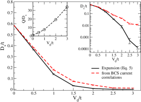
Figure 2: (Color online) Main panel: Comparison between the superfluid stiffness computed using Eq. (5) and its BCS counterpart as a function of disorder. Upper right inset: Same data plotted on a log-log scale to demonstrate increasing deviations for large $V_{0}/t$. Upper left inset: Ratio between anharmonic ($Q$) and quadratic coefficient ($D_{s}$) of the expansion Eq. (6) (with $Q/D_{s}=1.01$ at $V=0$). Note that for the given parameter set $\xi_{0}\approx 1a$ so that $J^{\prime}/J\approx Q/D_{s}$.

The coherence length has been determined from the decay of the gap amplitude correlations which yields $\xi_{0}\approx 1a$, so that for the present parameters $Q/D_{s}\approx J^{\prime}/J$. The upper left inset to Fig.2 shows the ratio $Q/D_{s}$ as obtained from the fit of $E(A)$ to Eq. (6). For increasing disorder $Q/D_{s}\approx J^{\prime}/J$ becomes strongly enhanced leading rapidly to a larger phase-fluctuation correction within the Hubbard as compared to the $XY$ model where $J^{\prime}/J=1$. Above a critical value of the disorder strength $V_{0}/t\approx 3$ a SC-I transition is obtained when $D_{s}=0$. Within an RPA analysis of the full model on small clusters we have also checked seibold that $\langle(\delta\theta)^{2}\rangle$ is increasing with disorder, however, the dependence on $V_{0}$ being much weaker than that for $Q/D_{s}$.

The above discussion shows that the $XY$ model fails in general to describe quantitatively corrections of the superfluid stiffness due to numerical differences in the quartic coefficient. Notwithstanding a disordered version of it can help to get some insight on the anomalously large increase of the $J^{\prime}/J$ ratio as a function of disorder. Let us consider for simplicity a one-dimensional XY-model in the presence of a constant gauge field, $H=\sum_{i}J_{i,i+1}(1-\cos(\theta_{i}-\theta_{i+1}-2A))$. In order to describe a disordered model we consider a random distribution of couplings $J_{i,i+1}$. To derive the coefficients $J,J^{\prime}$ of the expansion (6) we can use the fact that in 1D the current in each link, $j(A)$, must be conserved, so that $-J_{i,i+1}\sin(\theta_{i}-\theta_{i+1}-2A)=j(A)/2$. By inverting this relation, summing over the index $i$ and expanding $j(A)/2\approx JA-\frac{J^{\prime}}{6}A^{3}$ we then obtain that the coefficients are given by the spatial averages, $J^{-1}=\overline{1/J_{i,i+1}}$ (see also Ref. par98 ), and $J^{\prime}=J^{4}\;\overline{1/J_{i,i+1}^{3}}$. By computing for example the ratio $J^{\prime}/J$ for a Gaussian distribution of local coupling values one can see that it increases very rapidly as the distribution width increases, leading to a non-vanishing occurrence probability for very low values of $J_{i,i+1}$, which have a much stronger effect on $J^{\prime}$ than on $J$. As a byproduct this computation also shows the importance of phase relaxation, without which $J$ would be defined as $J=\overline{J_{i,i+1}}$. Obviously, in 2D the current in each link is not constant. Thus in principle the current would try to avoid links with very low $J_{ij}$ couplings to avoid coexistence of large phase change and large current, which from Fig. 1 seems to be indeed the case. However, these patterns have an almost one dimensional character so that the above argument could be still qualitatively correct even in 2D. Nevertheless the variation of local $J_{ij}$ values along the active paths (i.e. paths with current) can be smaller than along paths with vanishing current.

In conclusion, we have analyzed from a real space BdG approach for the attractive Hubbard model, the reaction of a strongly disordered SC system to an applied transverse vector potential. The first main result concerns the standard decoupling between transverse and longitudinal response which does not apply in the presence of disorder. We have evaluated the corrections of the superfluid stiffness to the dirty BCS limit (cf. Fig. 2) and obtained a strong reduction of the superfluid stiffness due to the relaxation of the order parameter phase for large disorder. We also find that the anharmonicity of the phase fluctuations is increased by disorder. Beyond mean-field, this enhances the effect of quantum fluctuations in producing a zero-temperature transition to a non-SC phase. Both effects can explain the deviations of the zero-temperature superfluid stiffness from the BCS dirty limit reported recently for strongly disordered NbN filmsmondal10 .

Secondly, our calculations have revealed that the stiffness for strong disorder is dominated by quasi one-dimensional percolative paths along sites with large gap parameters. In some sense this mimics the finding of Ref. IMFIM where the phase diagram of a model, similar to the present one in the large $U/t$ limit, has been analyzed within the so-called cavity mean-field approximation. Interestingly it was found that there is a regime of broken-replica symmetry where the partition function is determined by a small number of paths. Taking that a similar glassy physics is at work in our model, where the response is governed by a few number of percolative paths, then this should also appear in the distribution functions of order parameters and energy level spacings. An analysis of this issue is in progress.

References

- (1) B.Sacepe et al., Nature Communications 1, 140 (2010).
- (2) M. Mondal et al., Phys. Rev. Lett. 106 047001 (2011).
- (3) For a recent review see e.g. M. V. Feigel’man et al., Annals of Physics 325, 1368 (2010) and references therein.
- (4) M. P. A. Fisher, G. Grinstein and S. M. Girvin, Phys. Rev. Lett. 64, 587 (1990).
- (5) A. Ghosal, M. Randeria and N. Trivedi, Phys. Rev. B65, 014501 (2001).
- (6) M. V. Feigel’man et al., Phys. Rev. Lett. 98, 027001 (2007).
- (7) Y Dubi, Y. Meir and Y. Avishai, Nature 449, 876 (2007).
- (8) K. Bouadim et al., arXiv:1011.3275.
- (9) L. B. Ioffe and M. Mezard Phys. Rev. Lett. 105, 037001 (2010); M. V. Feigel’man, L. B. Ioffe, and M. Mézard Phys. Rev. B82, 184534 (2010).
- (10) P.G. de Gennes, Superconductivity in Metals and Alloys (Benjamin, New York, 1966).
- (11) J. R. Schrieffer, Theory Of Superconductivity (Perseus Books, Reading, 1999).
- (12) A. Paramekanti, N. Trivedi, M. Randeria, Phys. Rev. B 57, 11639 (1998).
- (13) S. Kirkpatrick, Rev. Mod. Phys. 45,574 (1973).
- (14) D. J. Scalapino, S. R. White and S. Zhang, Phys. Rev. B47, 7995 (1993).
- (15) W.Kohn, Phys. Rev. B133, A171 (1964)
- (16) L. Benfatto, A. Toschi, and S. Caprara, Phys. Rev. B. 69, 184510 (2004).
- (17) L. Benfatto et al., Phys. Rev. B 63, 174513 (2001).
- (18) G. Seibold, et al. in preparation.