Conditioned Poisson distributions
and the concentration of chromatic numbers

Abstract.

The paper provides a simpler method for proving a delicate inequality that was used by Achlioptis and Naor to establish asymptotic concentration for chromatic numbers of Erdös-Rényi random graphs. The simplifications come from two new ideas. The first involves a sharpened form of a piece of statistical folklore regarding goodness-of-fit tests for two-way tables of Poisson counts under linear conditioning constraints. The second idea takes the form of a new inequality that controls the extreme tails of the distribution of a quadratic form in independent Poissons random variables.

1. Introduction

Recently, AchlioptasNaor05AM established a most elegant result concerning colorings of the Erdös-Rényi random graph, which has vertex set $V=\{1,2,\dots,n\}$ and has each of the $\binom{n}{2}$ possible edges included independently with probability $d/n$, for a fixed parameter $d$. They showed that, as $n$ tends to infinity, the chromatic number concentrates (with probability tending to one) on a set of two values, which they specified as explicit functions of $d$. The main part of their argument used the “second moment method” [Alon and SpencerAlon and Spencer2000, Chapter 4] to establish existence of desired colorings with probability bounded away from zero. Most of their paper was devoted to a delicate calculation bounding the ratio of a second moment to the square of a first moment.

More precisely, A&N considered the quantity

$$A_{n}(c):=\frac{n^{k-1}}{k^{2n}}\left(1-\frac{1}{k}\right)^{-2nc}\sum_{\ell\in{\mathcal{H}}_{k}}\frac{n!}{\prod_{i,j}\ell_{ij}!}\left(1-\frac{2}{k}+\sum\nolimits_{i,j}\left(\frac{\ell_{ij}}{n}\right)^{2}\right)^{nc},$$

where ${\mathcal{H}}_{k}$ denotes the set of all $k\times k$ matrices with nonnegative entries for which each row and column sum equals $B:=n/k$. (With no loss of generality, A&N assumed that $n$ is an integer multiple of $k$.) They needed to show, for each fixed $k\geq 3$, that

(1) $$A_{n}(c)=O(1)\qquad\text{when $c<(k-1)\log(k-1)$.}$$

In this paper we show how the A&N calculations can be simplified by using results about conditioned Poisson distributions. More precisely, we show that the desired behaviour of $A_{n}(c)$ follows from a sharpening of a conditional limit theorem due to Haberman74book together with some elementary facts about the Poisson distribution.

In Section 2 we will establish some basic notation and record some elementary facts about the Poisson distribution. In Section 3 we will explain how $A_{n}(c)$ can be bounded by a conditional expectation of an exponential function of the classical goodness-of-fit statistic for two-way tables. We will outline our proof of (1), starting from a $\chi^{2}$ heuristic that can be sharpened (Section 4) into a rigorous proof that handles the contributions to $A_{n}(c)$ from all except some extreme values of $\ell$. To control the contributions from the extreme $\ell$ we will use an inequality (Lemma 2) that captures the large deviation behaviour of conditioned Poissons. The proof of the Lemma (in Section 5) is actually the most delicate part of our argument.

2. Facts about the Poisson distribution

Many of the calculations in our paper involve the convex function

(2) $$h(t)=(1+t)\log(1+t)-t\qquad\text{for $-1\leq t$},$$

which achieves its minimum value of zero at $t=0$. Near its minimum, $h(t)=t^{2}/2+O(|t|^{3})$. In fact, $h(t)=\tfrac{1}{2}t^{2}\psi(t)$ where $\psi$ is a decreasing function with $\psi(0)=1$ and $\psi^{\prime}(0)=-1/3$. See [page 312]PollardUGMTP for a simple derivation of these facts.

Define $\mathbb{N}_{0}=\{0,1,2,\dots\}$, the set of all nonnegative integers.

Lemma 1.

Suppose $W$ has a $\text{Poisson}(\lambda)$ distribution, with $\lambda\geq 1$.

1. If $\ell=\lambda+\lambda u\in\mathbb{N}_{0}$ then

   $$\sqrt{2\pi\lambda}\mathbb{P}\{W=\ell\} =\exp\left(-\lambda h(u)-\tfrac{1}{2}\log(1+u)+O(1/\ell)\right)$$

   $$=\exp\left(-\tfrac{1}{2}\lambda{u^{2}}+O\left(|u|+\lambda|u|^{3}\right)\right).$$

2. $\mathbb{P}\{W=\ell\}\leq\exp(-\lambda h(u))$ for all $\ell=\lambda(1+u)\in\mathbb{N}_{0}$.

3. For all $w\geq 0$,

   $$\mathbb{P}\{|W-\lambda|\geq\lambda w\} \leq 2\exp(-\lambda h(w))=2\exp\left(-\tfrac{1}{2}\lambda{w^{2}}+O\left(\lambda|w|^{3}\right)\right)$$

Proof.

By Stirling’s formula,

$$\log(\ell!/\sqrt{2\pi})=(\ell+\tfrac{1}{2})\log(\ell)-\ell+r_{\ell}\qquad\text{where }\frac{1}{12\ell+1}\leq r_{\ell}\leq\frac{1}{12\ell}.$$

Thus

$$\log\bigl{(}\sqrt{2\pi\lambda}\mathbb{P}\{W=\ell\}\bigr{)} =-\lambda+\ell\log(\lambda)-\log(\ell!/\sqrt{2\pi})+\tfrac{1}{2}\log(\lambda)$$

$$=-\lambda h(u)-\tfrac{1}{2}\log(1+u)+O(\ell^{-1}),$$

which gives (i).

For (ii), first note that $\mathbb{P}\{W=0\}=e^{-\lambda}=\exp(-\lambda h(-1))$. For $\ell\geq 1$ we have

$$\log\left(\sqrt{2\pi}\mathbb{P}\{W=\ell\}\right) =-\lambda+\ell\log(\lambda)-(\ell+\tfrac{1}{2})\log(\ell)+\ell-r_{\ell}$$

$$\leq-\lambda+\ell\log(\lambda)-\ell\log(\ell)+\ell=\lambda h(u).$$

Inequality (iii) comes from two appeals to the usual trick with the moment generating function $\mathbb{P}e^{tW}=\exp(\lambda(e^{t}-1))$. For $w\geq 0$,

$$\mathbb{P}\{W\geq\lambda+\lambda w\}\leq\inf_{t\geq 0}\mathbb{P}e^{t(W-\lambda-\lambda w)}=\inf_{t\geq 0}\exp\left(-t\lambda(1+w)+\lambda(e^{t}-1)\right)$$

The infimum is achieved at $t=\log(1+w)$, giving the bound $\exp(-\lambda h(w))$. Similarly

$$\mathbb{P}\{W\leq\lambda-\lambda w\}\leq\inf_{t\geq 0}\mathbb{P}e^{t(\lambda-\lambda w-W)}=\inf_{t\geq 0}\exp\left(t(\lambda-\lambda w)+\lambda(e^{-t}-1)\right)$$

with the infimum achieved at $t=-\log(1-w)$ if $0\leq w<1$ or as $t\to\infty$ if $w=1$. The inequality is trivial for $w>1$. ∎

3. Heuristics and an outline of the proof of (1)

We first show that $A_{n}(c)$ is almost a conditional expectation involving a set of independent random variables, $Y=\{Y_{ij}:1\leq i,j,\leq k\}$, each distributed Poisson$(\lambda_{ij})$ with $\lambda_{ij}=n/k^{2}$ for all $i,j$. For $\ell\in{\mathcal{H}}_{k}$,

$$p(\ell):=\mathbb{P}\{Y=\ell\}=\frac{e^{-n}(n/k^{2})^{n}}{\prod_{i,j}\ell_{ij}!}=\frac{n!}{\prod_{i,j}\ell_{ij}!}\frac{n^{n}e^{-n}}{n!}k^{-2n}$$

The standardized variables $X_{ij}:=(Y_{ij}-\lambda_{ij})/\sqrt{\lambda_{ij}}$ are approximately independent standard normals.

As we show in Section 4, the quantity

$$\beta_{n}:=n^{(2k-1)/2}\mathbb{P}\{Y\in{\mathcal{H}}_{k}\}$$

converges to a strictly positive constant as $n$ tends to infinity. Thus

$$p_{2}(\ell):=\mathbb{P}\{Y=\ell\mid Y\in{\mathcal{H}}_{k}\} =p(\ell)/\mathbb{P}\{Y\in{\mathcal{H}}_{k}\}$$

$$=n^{k-1}k^{-2n}\dfrac{n!}{\prod_{i,j}\ell_{ij}!}\dfrac{n^{n+1/2}e^{-n}}{n!\,\beta_{n}}.$$

By Stirling’s approximation, the final fraction converges to a nonzero constant. The quantity $A_{n}(c)$ is bounded by a constant multiple of

(3) $$\left(1-\frac{1}{k}\right)^{-2nc}\sum\nolimits_{\ell\in{\mathcal{H}}_{k}}p_{2}(\ell)\left(1-\frac{2}{k}+\sum\nolimits_{i,j}(\ell_{ij}/n)^{2}\right)^{nc}.$$

That is, for some constant $C_{0}$,

$$A_{n}(c)\leq C_{0}\left(1-\frac{1}{k}\right)^{-2nc}\mathbb{P}_{2}\left(1-\frac{2}{k}+\sum\nolimits_{i,j}(Y_{ij}/n)^{2}\right)^{nc},$$

where $\mathbb{P}_{2}(\cdot)$ denotes expectations with respect to the conditional probability distribution $\mathbb{P}(\cdot\mid Y\in{\mathcal{H}}_{k})$.

Note the similarily to the usual chi-squared goodness-of-fit statistic,

$$|X|^{2}:=\sum\nolimits_{i,j}X_{ij}^{2}=-n+nk^{2}\sum\nolimits_{i,j}(Y_{ij}/n)^{2}.$$

The quantity in (3) equals the $\mathbb{P}_{2}$ expectation of

$$\left(1-\frac{1}{k}\right)^{-2nc}\left(\left(1-\frac{1}{k}\right)^{2}+\frac{|X|^{2}}{nk^{2}}\right)^{nc}\leq\exp\left(\frac{c|X|^{2}}{(k-1)^{2}}\right).$$

Our task has become: for a fixed $J_{k}:=c/(k-1)^{2}<\rho_{k}:=\log(k-1)/(k-1)$, show that

(4) $$\mathbb{P}_{2}\exp\left({J_{k}|X|^{2}}\right)=O(1)\qquad\text{as $n\to\infty$. }$$

Under $\mathbb{P}_{2}$, the random vector $X$ has a limiting normal distribution ${\mathcal{N}}$ that concentrates on a $(k-1)^{2}$-dimensional subspace of $\mathbb{R}^{k\times k}$. The random variable $|X|^{2}$ has an asymptotic $\chi^{2}_{R}$ distribution with $R=(k-1)^{2}$. If we could assume that $|X|^{2}$ were exactly $\chi^{2}_{R}$-distributed, we could bound the conditional expectation in (4) by a constant times

$$\int_{0}^{\infty}t^{R/2-1}\exp\left(ct/R-t/2)\right)\,dt,$$

which would be finite for $c<R/2=(k-1)^{2}/2$.

To make the argument rigorous we will need to consider the contributions from the large $|Y_{ij}-n/k^{2}|$’s more carefully. As a special case of Theorem 3 in Section 4, we know that for each fixed $\theta>1$ there exists a $\delta=\delta_{\theta}$ for which

(5) $$\mathbb{P}_{2}\exp\left(J_{k}|X|^{2}\right)\{|X|\leq\delta\sqrt{n}\}\leq\theta{\mathcal{N}}\exp(\theta^{2}J_{k}|x|^{2}).$$

The expectation with respect to the normal distribution ${\mathcal{N}}$ can be bounded as in the previous paragraph because $|x|^{2}\sim\chi^{2}_{(k-1)^{2}}$ under ${\mathcal{N}}$.

To control the contribution from $\{|X|>\delta\sqrt{n}\}$ it is notationally cleaner to work with the variables $U_{ij}:=(Y_{ij}-\lambda_{ij})/\lambda_{ij}$, that is, $U=kX/\sqrt{n}$. Write ${\mathcal{U}}$ for the set of all $u$ in $\mathbb{R}^{k\times k}$ for which $\lambda_{ij}(1+u_{ij})\in\mathbb{N}_{0}$ for all $i,j$ and (because $Y$ is constrained to lie in ${\mathcal{H}}_{k}$),

(6) $$-1\leq u_{ij}\leq k-1\qquad\text{and}\quad\sum\nolimits_{i}u_{ij}=0=\sum\nolimits_{j}u_{ij}.$$

We need to bound

$$\mathbb{P}\exp\left(nJ_{k}|U|^{2}/k^{2}\right)\{|U|>k\delta\}/\mathbb{P}\{Y\in{\mathcal{H}}_{k}\}$$

$$\qquad=O(n^{(2k-1)/2})\sum\nolimits_{u\in{\mathcal{U}}}\{|u|>k\delta\}\mathbb{P}\{U=u\}\exp(nJ_{k}|u|^{2}/k^{2})$$

From Lemma 1,

$$\mathbb{P}\{U=u\}\leq\prod\nolimits_{ij}\exp(-nh(u_{ij})/k^{2}),$$

which leads us to the task of showing that

(7) $$\sum\nolimits_{u\in{\mathcal{U}}}\{|u|>k\delta\}\exp\left(\frac{n}{k^{2}}\sum\nolimits_{ij}\left(J_{k}u_{ij}^{2}-h(u_{ij})\right)\right)=O(n^{-(2k-1)/2}).$$

Here we can make use of an inequality (proved in Section 5) that controls the exponent in (7). Recall that $h(t)=(1+t)\log(1+t)-t$ and $\rho_{k}=\log(k-1)/(k-1)$.

Lemma 2.

For each $u=(u_{1},\dots,u_{k})\in\mathbb{R}^{k}$ for which $\sum_{j}u_{j}=0$ and $-1\leq u_{j}\leq k-1$ for all $j$, we have $\sum_{j}h(u_{j})\geq\rho_{k}\sum_{j}u_{j}^{2}$.

When invoked for the sum over $j$ for each fixed $i$, the Lemma bounds (7) by

$$\sum\nolimits_{u\in{\mathcal{U}}}\{|u|>k\delta\}\exp\left(-n\epsilon_{0}|u|^{2}\right)\qquad\text{where $\epsilon_{0}:=(\rho_{k}-J_{k})/k^{2}>0$.}$$

The set $\{u\in{\mathcal{U}}:2^{b}k\delta<|u|\leq 2^{b+1}k\delta\}$ has cardinality of order $O((n2^{b})^{k^{2}})$. The last sum is less than

$$O(n^{k^{2}})\sum\nolimits_{b\in\mathbb{N}_{0}}\exp\left(k^{2}b-n\epsilon_{0}4^{b}\right)$$

which decreases exponentially fast with $n$.

The bound asserted in (4) follows.

4. Limit theory for conditioned Poisson distributions

The main result in this Section is Theorem 3, which shows that the contributions to the left-hand side of (4) from a large range of $X$ values can actually be bounded using the $\chi^{2}$-approximation.

Suppose $\mathbf{Y}=(Y_{1},\dots,Y_{q})$ is a vector of independent random variables with $Y_{i}$ distributed $\text{Poisson}(\lambda_{i})$. Define

$$\lambda:=(\lambda_{1},\dots,\lambda_{q})\qquad\text{and}\quad D:=\mbox{diag}(\lambda^{1/2}_{1},\dots,\lambda^{1/2}_{q}).$$

For the rest of this section assume that $\nu:=\sum_{i}\lambda_{i}$ converges to infinity and that there exists some fixed constant $\tau>0$ for which

(8) $$\nu\geq\max\nolimits\lambda_{i}\geq\min\nolimits_{i}\lambda_{i}\geq\tau\nu.$$

The various constants that appear throughout the section might depend on $\tau$.

Suppose ${\mathbf{V}}_{1},\dots,{\mathbf{V}}_{s}$ are fixed vectors in ${\mathbb{Z}}^{q}$ that are linearly independent, spanning a subspace ${\mathcal{L}}$ of $\mathbb{R}^{q}$. The linear independence implies the existence of nonzero constants $C_{1}$ and $C_{2}$ for which

(9) $$C_{1}\max\nolimits_{\alpha}|t_{\alpha}|\leq|\sum\nolimits_{\alpha}t_{\alpha}V_{\alpha}|\leq C_{2}\max\nolimits_{\alpha}|t_{\alpha}|\qquad\text{for all $t_{\alpha}\in\mathbb{R}$}.$$

We also assume that

(10) $${\mathbb{Z}}^{q}\cap({\mathbf{\lambda}}\oplus{\mathcal{L}})\neq\emptyset.$$

Under similar assumptions, [Chapter 1]Haberman74book proved a central limit theorem for the random vector $X:=D^{-1}(Y-\lambda)$ conditional on the event $\{Y\in\lambda\oplus{\mathcal{L}}\}$. The limit distribution ${\mathcal{N}}_{\lambda}$ is that of a $N(0,I_{q})$ conditioned to lie in the $s$-dimensional subspace $D^{-1}{\mathcal{L}}$. More precisely, ${\mathcal{N}}_{\lambda}$ has density $\phi(x)=(2\pi)^{-s/2}\exp(-\left|x\right|^{2}/2)$ with respect to Lebesgue measure $\mathbf{m}_{\lambda}$ on the subspace $D^{-1}{\mathcal{L}}$.

We will write $\mathbb{Q}(\cdot)$ to denote expectations under $\mathbb{P}(\cdot\mid Y\in\lambda\oplus{\mathcal{L}}\}$. That is, for the conditional expectation of a function of $Y$,

$$\mathbb{Q}f(Y)=\frac{\mathbb{P}f(Y)\{Y\in\lambda\oplus{\mathcal{L}}\}}{\mathbb{P}\{Y\in\lambda\oplus{\mathcal{L}}\}}.$$

For the calculations leading to inequality (5), the $q\times 1$ vectors are more naturally written as $k\times k$ tables. The vector of means becomes a table $\lambda=\{\lambda_{ij}:1\leq i,j\leq k\}$ with $\lambda_{ij}=n/k^{2}$ for all $i,j$. The constraints on row and column sums can be written using the $2k$ tables with ones in a single row or column, zeros elsewhere, but only $2k-1$ of those tables are linearly independent. Thus $q=k^{2}$ and $s=k^{2}-(2k-1)=(k-1)^{2}$ and $\nu=n$. The $\mathbb{Q}$ in this Section corresponds to the $\mathbb{P}_{2}$ from Section 3.

For each $w\in{\mathbb{Z}}^{s}$ define $\mathbf{z}_{w}:=\sum_{\alpha\leq s}w_{\alpha}{\mathbf{V}}_{\alpha}$, a point of ${\mathbb{Z}}^{q}$. The key idea in Haberman’s argument is that the space ${\mathcal{L}}$ is partitioned into disjoint boxes

$$B_{w}:=\{\sum\nolimits_{i\leq s}t_{i}{\mathbf{V}}_{i}:\lfloor t_{i}\rfloor=w_{i}\}=\mathbf{z}_{w}\oplus B_{0}\qquad\text{for $w\in{\mathbb{Z}}^{s}$},$$

each containing the same number, $\kappa_{V}$, of lattice points from ${\mathbb{Z}}^{q}$. Assumption (10) ensures that $\kappa_{V}>0$.

Theorem 3.

Suppose $g$ is a uniformly continuous, increasing function. Then for each $\theta>1$ there exists a $\delta>0$ and a subset ${\mathcal{L}}_{\delta}$ of ${\mathcal{L}}$ for which

1. $\{x\in D^{-1}{\mathcal{L}}:|x|\leq\delta\sqrt{\nu}\}\subseteq D^{-1}{\mathcal{L}}_{\delta}$

2. $\mathbb{Q}\exp\left(g(|X|^{2})\right)\{X\in D^{-1}{\mathcal{L}}_{\delta}\}\leq\theta{\mathcal{N}}_{\lambda}\exp\left(g(\theta^{2}|x|^{2})\right)\{x\in D^{-1}{\mathcal{L}}_{\delta}/\theta\}$

The proof of the Theorem will be given at the end of this Section, as the culmination of a sequence of lemmas based on the elementary facts from Section 2. We first show that most of the contributions to the $\mathbb{P}_{2}$ and ${\mathcal{N}}_{\lambda}$ probabilities come from a large, bounded subset of ${\mathcal{L}}$.

Lemma 4.

For each $\delta>0$ define ${\mathcal{W}}_{\delta}:=\{w\in{\mathbb{Z}}^{s}:\max_{\alpha}|w_{\alpha}|\leq\delta\nu\}$ and ${\mathcal{L}}_{\delta}:=\cup_{w\in{\mathcal{W}}_{\delta}}B_{w}$. There exists a constant $C_{\delta}>0$ for which

$$\mathbb{P}\{Y\notin\lambda\oplus{\mathcal{L}}_{\delta}\}+{\mathcal{N}}_{\lambda}(D^{-1}{\mathcal{L}}_{\delta}^{c})\}=O(e^{-C_{\delta}\nu}).$$

Proof.

If $y\in\lambda\oplus({\mathcal{L}}\backslash{\mathcal{L}}_{\delta})$ then $y-\lambda\in\mathbf{z}_{w}\oplus B_{0}$ for some $w$ with $\max_{\alpha}|w_{\alpha}|>\delta\nu$, which implies

$$\sqrt{k}\max_{i}|y_{i}-\lambda_{i}|\geq|y-\lambda|\geq|\mathbf{z}_{w}|-\text{diam}(B_{0})\geq C_{1}\delta\nu-C_{4}.$$

Define $\delta_{0}:=C_{1}\delta/(2\sqrt{k})$. When $\nu$ is large enough we have $(C_{1}\delta\nu-C_{4})/\sqrt{k}>\delta_{0}\nu\geq\delta_{0}\max_{i}\lambda_{i}$, so that

$$\mathbb{P}\{Y\notin\lambda\oplus{\mathcal{L}}_{\delta}\}\leq\sum\nolimits_{i}\mathbb{P}\{|Y_{i}-\lambda_{i}|>\delta_{0}\lambda_{i}\}.$$

Invoke Lemma 1 to bound the $i$th summand by $2\exp\left(-\lambda_{i}\delta_{0}^{2}/2+O(\delta_{0}^{3}\lambda_{i})\right)$. With a possible decrease in $\delta_{0}$ we can ensure that the $\lambda_{i}\delta_{0}^{2}/2$ is at least twice the other contribution to the exponent.

Similarly, if ${\mathbf{x}}\in D^{-1}({\mathcal{L}}\backslash{\mathcal{L}}_{\delta})$ and $\nu$ is large enough then $|{\mathbf{x}}|>\delta_{0}\sqrt{\nu}$ and the contribution from ${\mathcal{N}}_{\lambda}$ is bounded by a sum of tail probabilities for the standard normal. ∎

Next we use Lemma 1 to get good pointwise approximations for $\mathbb{P}\{Y=\ell\}$ when $|\ell-\lambda|$ is not too large.

Lemma 5.

For each $\theta>1$ there exists a $\delta>0$ such that, for all $\ell=\lambda+Dx$ in $\mathbb{N}_{0}^{q}$ for which $\max_{i}\lambda_{i}^{-1}|\ell_{i}-\lambda_{i}|\leq\delta$,

$$\theta^{-1}\phi\left(\theta{\mathbf{x}}\right)\leq\nu^{q/2}\mathbb{P}\{\mathbf{Y}=\ell\}/\gamma(\lambda)\\ \leq\theta\phi\left({\mathbf{x}}/\theta\right)$$

where $\gamma(\lambda):=(2\pi)^{s/2}\prod\nolimits_{i}(2\pi\lambda_{i}/\nu)^{-1/2}$, a factor that stays bounded away from zero and infinity as $\nu\to\infty$.

Proof.

From Lemma 1,

$$\left(\prod\nolimits_{i}\sqrt{2\pi\lambda_{i}}\right)\mathbb{P}\{\mathbf{Y}=\ell\}=\prod\nolimits_{i}\exp\left(-\tfrac{1}{2}x_{i}^{2}+r_{i}\right)$$

where, for some constant $C_{3}$,

$$|r_{i}|\leq C_{3}(|x_{i}|+|x_{i}|^{3})/\sqrt{\nu}\leq C_{3}\delta(1+x_{i}^{2}).$$

The asserted inequalities follow if $\delta$ is small enough. ∎

Next we sum over the pointwise approximations to get bounds for the probability that $Y$ lies in one of the boxes that partition $\lambda\oplus{\mathcal{L}}$. The sum for the box $\lambda\oplus B_{w}$ will run over the lattice points of the form $\lambda+Dx$ with $x$ in the set

$${\mathcal{X}}_{w}=\{x\in D^{-1}B_{w}:\lambda+Dx\in\mathbb{N}_{0}^{q}\}.$$

Lemma 6.

For each $\theta>1$ there exists a $\delta>0$ such that, for all $w$ in ${\mathcal{W}}_{\delta}$ and $\nu$ large enough,

$$\theta^{-1}{\mathcal{N}}_{\lambda}\left(D^{-1}B_{w}\theta\right) \leq\nu^{(q-s)/2}\mathbb{P}\{Y\in\lambda\oplus B_{w}\}/\beta(\lambda)$$

$$\leq\theta{\mathcal{N}}_{\lambda}\left(D^{-1}B_{w}/\theta\right)$$

where $\beta(\lambda)$ is a factor that stays bounded away from zero and infinity as $\nu\to\infty$.

Proof.

As the proofs for the two inequalities are similar, we consider only the upper bound.

Define ${\mathbf{x}}_{w}:=D^{-1}\mathbf{z}_{w}$. By inequality (9) we have $|\mathbf{z}_{w}|\leq C_{2}\delta\nu$ and hence $|{\mathbf{x}}_{w}|\leq C_{4}\delta\sqrt{\nu}$ for some constant $C_{4}$. Similarly, for each $\mathbf{y}=\lambda+D{\mathbf{x}}$ in $\lambda\oplus B_{w}$ we have $|y-\lambda-\mathbf{z}_{w}|$ bounded by a constant, which implies $|{\mathbf{x}}-{\mathbf{x}}_{w}|\leq C_{5}/\sqrt{\nu}$ and hence

$$|\,|{\mathbf{x}}|^{2}-|{\mathbf{x}}_{w}|^{2}\,|\leq\delta_{0}:=C_{5}^{2}/\nu+2(C_{5}/\sqrt{\nu})C_{4}\delta\sqrt{\nu}.$$

It follows that for each $\epsilon>0$ and $\sigma$ close enough to $1$,

$$\sup\{|\phi({\mathbf{x}}/\sigma)/\phi({\mathbf{x}}_{w}/\sigma)-1|:{\mathbf{x}}\in D^{-1}B_{w}\}<\epsilon$$

if $\nu$ is large enough and $\delta$ is small enough.

Taking $\sigma$ equal to the $\theta$ from Lemma 5 we then have

$$\mathbb{P}\{Y\in\lambda\oplus B_{w}\} =\sum\nolimits_{x\in{\mathcal{X}}_{w}}\mathbb{P}\{Y=\lambda+Dx\}$$

$$\leq\theta\gamma(\lambda)\nu^{-q/2}\sum\nolimits_{x\in{\mathcal{X}}_{w}}\phi(x/\theta)$$

$$\leq\theta\gamma(\lambda)\nu^{-q/2}\kappa_{V}(1+\epsilon)\phi({\mathbf{x}}_{w}/\theta).$$

Similarly,

$${\mathcal{N}}_{\lambda}(D^{-1}B_{w}/\theta) =\int\{\theta\mathbf{t}\in D^{-1}B_{w}\}\phi(\mathbf{t})\mathbf{m}_{\lambda}(d\mathbf{t})$$

$$=\theta^{-s}\int\{{\mathbf{x}}\in D^{-1}B_{w}\}\phi({\mathbf{x}}/\theta)\mathbf{m}_{\lambda}(d{\mathbf{x}})$$

$$\geq\theta^{-s}\phi({\mathbf{x}}_{w}/\theta)(1-\epsilon)\mathbf{m}_{\lambda}(D^{-1}B_{0}).$$

The invariance properties of Lebesgue measure imply existence of some function $\mu(\lambda)$ that stays bounded away from zero and infinity as $\nu$ tends to infinity, for which $\mathbf{m}_{\lambda}(D^{-1}B_{0})=\nu^{-s/2}\mu(\lambda)$. Thus

$$\mathbb{P}\{Y\in\lambda\oplus B_{w}\}\leq\theta^{s+1}\frac{1+\epsilon}{1-\epsilon}\nu^{-(q-s)/2}\frac{\kappa_{V}\gamma(\lambda)}{\mu(\lambda)}{\mathcal{N}}_{\lambda}(D^{-1}B_{w}/\theta).$$

Choose $\epsilon$ small enough and replace $\theta$ by a value closer to $1$ to get the upper half of the asserted inequality, with $\beta(\lambda)=\kappa_{V}\gamma(\lambda)/\mu(\lambda)$. ∎

Corollary 7.

$\mathbb{P}\{Y\in\lambda\oplus{\mathcal{L}}\}=\nu^{-(q-s)/2}\left(\beta(\lambda)+o(1)\right)$

Proof.

From Lemmas 4 and 6, for each $\theta>1$,

$$\mathbb{P}\{Y\in\lambda\oplus{\mathcal{L}}\} =\mathbb{P}\{Y\notin\lambda\oplus{\mathcal{L}}_{\delta}\}+\sum\nolimits_{w}\{w\in{\mathcal{W}}_{\delta}\}\mathbb{P}\{Y\in\lambda\oplus B_{w}\}$$

$$\leq O(e^{-C_{\delta}\nu})+\theta\beta(\lambda)\nu^{-(q-s)/2}\sum\nolimits_{w}\{w\in{\mathcal{W}}_{\delta}\}{\mathcal{N}}_{\lambda}\left(D^{-1}B_{w}/\theta\right)$$

$$\leq\theta\nu^{-(q-s)/2}\left(\beta(\lambda)+o(1)\right)$$

The argument for the lower bound is similar. ∎

Corollary 8.

For all $\nu$ large enough,

$$\theta^{-1}{\mathcal{N}}_{\lambda}(D^{-1}B_{w}\theta)\leq\mathbb{Q}\{Y\in\lambda\oplus B_{w}\}\leq\theta{\mathcal{N}}_{\lambda}(D^{-1}B_{w}/\theta)$$

for all $w\in{\mathcal{W}}_{\delta}$.

We now have all the facts needed to prove Theorem 3. The argument is a slight modification of the method used to prove Lemma 6. Start with the $\delta$ and ${\mathcal{L}}_{\delta}$ from that Lemma. Assertion (i), modulo an unimportant constant, was established at the start of the proof of the Lemma.

Define $f(x):=\exp(g(|x|^{2}))$. From the proof of the Lemma we know that $|\,|{\mathbf{x}}|^{2}-|{\mathbf{x}}_{w}|^{2}\,|\leq\delta_{0}$. By uniform continuity of $g$, if $\delta$ is small enough we then have

$$|g(|x|^{2}/\sigma^{2})-g(|x_{w}|^{2}/\sigma^{2})|<\epsilon\qquad\text{all $x\in D^{-1}B_{w}$, all $\sigma\approx 1$}$$

and hence

$$e^{-\epsilon}f(x_{w}/\sigma)\leq f(x/\sigma)\leq e^{\epsilon}f(x_{w}/\sigma)\qquad\text{all $x\in D^{-1}B_{w}$, all $\sigma\approx 1$.}$$

Use the bounds on $f$ on $D^{-1}B_{w}$ to deduce that

$$\mathbb{Q}f(X)\{Y\in\lambda\oplus B_{w}\} \leq e^{\epsilon}f(x_{w})\mathbb{Q}\{Y\in\lambda\oplus B_{w}\}$$

$$\leq e^{\epsilon}f(\theta x_{w})\theta{\mathcal{N}}_{\lambda}(D^{-1}B_{w}/\theta)\qquad\text{as $g$ is increasing}$$

$$\leq e^{2\epsilon}\theta{\mathcal{N}}_{\lambda}f(\theta x)\{x\in D^{-1}B_{w}/\theta\}$$

Sum over $w$ in ${\mathcal{W}}_{\delta}$. to complete the argument.

5. Proof of Lemma 2

At a key step in the argument we will need the inequality

(11) $$\psi(t)\geq 2\log(1+2t)/(1+2t)\qquad\text{for all $t\geq 0$},$$

for which, unfortunately, we have no direct analytic proof. However, the assertion is trivially true near the origin because the lower bound tends to zero as $t$ tends to zero. For large $t$ the ratio of $\psi(t)$ to the lower bound tends to $2$. For intermediate values we have only a proof based on an analytic bound on derivatives together with numerical calculation on a suitably fine grid. It would be satisfying to have a completely analytic proof for (11).

Define $g_{k}(s):=h(s)-\rho_{k}s^{2}$. We need to show that the function $G_{k}(u):=\sum\nolimits_{j\leq k}g_{k}(u_{j})$ is nonnegative on the constraint set. Suppose the minimum is achieved at $t=(t_{1},\dots,t_{k})$. Without loss of generality, we may suppose $-1\leq t_{1}\leq t_{2}\leq\dots\leq t_{k}\leq k-1$. We cannot have $t_{1}=-1$ because $h^{\prime}(-1)=\infty$. Indeed,

$$g_{k}(t_{1}+\epsilon)+g_{k}(t_{k}-\epsilon)-g_{k}(t_{1})-g_{k}(t_{k})=\epsilon\log\epsilon+O(\epsilon),$$

which would be negative for small $\epsilon>0$. It then follows that $t_{k}<k-1$ for otherwise the constraint $\sum_{j}t_{j}=0$ would force $t_{j}=-1$ for $j<k$.

Use Lagrange multipliers (or argue directly regarding the first order effects of perturbations $\epsilon$ with $\sum\nolimits_{j}\epsilon_{j}=0$) to deduce existence of some constant $\theta$ for which $g^{\prime}_{k}(t_{j})=\theta$ for all $j$.

Note that $g^{\prime}_{k}(s)=\log(1+s)-2\rho_{k}s$ is concave (because $g^{\prime\prime}(s)$ is decreasing) with $g^{\prime}_{k}(0)=0$ and $g^{\prime\prime}_{k}(0)=1-2\rho_{k}>0$. It follows that $\theta\leq 0$ and that there are numbers $-1<a_{\theta}\leq 0\leq b_{\theta}<k-1$ with $g^{\prime}_{k}(a_{\theta})=\theta=g^{\prime}_{k}(b_{\theta})$ such that $t_{j}$ equals $j=a_{\theta}$ for $j\leq k-r$ and $b_{\theta}$ otherwise. That is $(k-r)a_{\theta}+rb_{\theta}=0$ and $G_{k}(t)=rg_{k}(b_{\theta})+(k-r)g_{k}(a_{\theta})$. Thus it suffices for us to show that the functions

$$M_{r,k}(b):=rg_{k}(b)+(k-r)g_{k}(-rb/(k-r))\qquad\text{for $0\leq b<(k-r)/r$}$$

are nonnegative for $r=1,2,\dots,k-2$.

For $r\geq 2$ and $0\leq b\leq(k-2)/2$, inequality (11) shows that $g_{k}(b)$ is nonnegative:

$$g_{k}(b) =b^{2}\left(\frac{1}{2}\psi(b)-2\rho_{k}\right)\geq b^{2}\left(\dfrac{\log(1+2b)}{1+2b}-\dfrac{\log(k-1)}{k-1}\right)\geq 0$$

because $b\mapsto\log(1+2b)/(1+2b)$ is a decreasing function. The function $M_{r,k}(b)$ is then a sum of nonnegative functions on $[0,(k-r)/r]$.

It remains only to consider the case where $r$ equals $1$. To simplify notation, write $k_{1}$ for $k-1$ and abbreviate $M_{1,k}$ to $M_{k}$. That is,

$$M_{k}(b) =h(b)+k_{1}h(-b/k_{1})-\rho_{k}\left(b^{2}+k_{1}(b/k_{1})^{2}\right)$$

$$=(1+b)\log(1+b)+(k_{1}-b)\log(1-b/k_{1})-k\rho_{k}b^{2}/k_{1},$$

whence

$$M_{k}^{\prime}(b) =\log\left(\frac{1+b}{1-b/k_{1}}\right)-\frac{2k\rho_{k}b}{k_{1}},\qquad M_{k}^{\prime\prime}(b)=\frac{k}{(1+b)(k_{1}-b)}-\frac{2k\rho_{k}}{k_{1}}.$$

Notice that $M_{k}^{\prime\prime}(b)\geq 0$ except on an interval  $I_{k}:=(b_{k},b_{k}^{\prime})$ in which the inequality $2(1+b)(k_{1}-b)>k_{1}/\rho_{k}$ holds.

For $k=3$ or $4$ the interval $I_{k}$ is empty. The functions $M_{3}$ and $M_{4}$ are convex. They achieve their minima of zero at $b=0$ because $M_{k}^{\prime}(0)=0$.

For $k\geq 5$, the interval $I_{k}$ is nonempty. The derivative $M_{k}^{\prime}(b)$ achieves its maximum value at $b=b_{k}$ and its the minimum value at $b_{k}^{\prime}$. For $k=5$ we have $b_{5}^{\prime}\approx 2.19$ and $M_{5}^{\prime}(b_{5}^{\prime})\approx 0.055$. Thus $M_{5}$ is an increasing function on $[0,4]$, achieving its minimum value of zero at $b=0$.

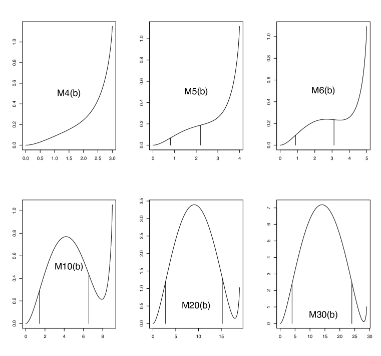
Figure 1. Plots of $M_{k}(b)$ for various values of $k$. The vertical lines mark off the intervals $I_{k}$ where the functions are concave.

For $k\geq 6$ a more delicate analysis is required. The function $M_{k}$ is concave on the segment $I_{k}$ and convex on each of the segments $[0,b_{k}]$ and $[b_{k}^{\prime},k_{1}]$. The global minimum is achieved either at $b=0$, with $M_{k}(0)=0$, or at the local minimum $b^{*}\in(b_{k}^{\prime},k_{1})$ where $M_{k}^{\prime}(b^{*})=0$ and $M_{k}^{\prime\prime}(b^{*})>0$. From the change in sign of the derivative,

$$M_{k}^{\prime}(k_{1}-1) =2\log(k_{1})/k_{1}^{2}>0\qquad\text{for all $k$}$$

$$M_{k}^{\prime}(k_{1}-2) =\frac{2(k_{1}+2)\log(k_{1})}{k_{1}^{2}}+\log\left(\frac{k_{1}-1}{2k_{1}}\right)<0\qquad\text{for $k\geq 6$},$$

we deduce that $k_{1}-2<b^{*}<k_{1}-1$. The convexity of $M_{k}$ on $[b_{k}^{\prime},k_{1}]$ then gives a linear lower bound,

$$M_{k}(b^{*}) \geq M_{k}(k_{1}-1)+(b^{*}-k_{1}+1)M_{k}^{\prime}(k_{1}-1)$$

$$\geq\dfrac{k_{1}-1}{k_{1}^{2}}\log(k_{1})-\dfrac{2\log(k_{1})}{k_{1}^{2}}$$

$$\geq 0\qquad\text{for $k\geq 4$}.$$

It follows that $M_{k}$ is nonnegative also for $k\geq 6$.

References

[\citeauthoryearAchlioptis and NaorAchlioptis and
Naor2005]
Achlioptis, D. and A. Naor (2005).
The two possible values of the chromatic number of a random graph.
Annals of Mathematics162, 1335–1351.
[\citeauthoryearAlon and SpencerAlon and
Spencer2000]
Alon, N. and J. H. Spencer (2000).
The Probabilistic Method (second ed.).
Wiley.
[\citeauthoryearHabermanHaberman1974]
Haberman, S. J. (1974).
The Analysis of Frequency Data.
University of Chicago Press.
[\citeauthoryearPollardPollard2001]
Pollard, D. (2001).
A User’s Guide to Measure Theoretic Probability.
Cambridge University Press.