Abstract

Double-well optical lattices are considered, each cite of which is formed by a double-well potential. The lattice is assumed to be in an insulating state and order and disorder are defined with respect to the displacement of atoms inside the double-well potential. It is shown that in such lattices, in addition to purely ordered and disordered states, there can exist an intermediate mixed state, where, inside a generally ordered lattice, there appear disordered regions of mesoscopic size.

E-mail: yukalov@theor.jinr.ru

1 Introduction

Cold atoms, loaded into optical lattices, form the systems that are unique with regard to the controllability of their properties (see the review articles [1-5] and references therein). One can vary the sorts of atoms as well as the lattice types and lattice spacing. For the given kind of atoms, one can vary their interactions by means of the Feshbach resonance techniques [5-7]. It is also possible to change the lattice properties by imposing external fields or shaking the lattice. This is why, one is able to create a variety of different system states in the lattice [1-5].

A special type of lattices are the double-well lattices, whose experimental realization has become possible in recent years [8-12]. In such lattices, each lattice site is formed by a double-well potential, which makes it feasible to create novel states that would be impossible in the standard single-well lattices. The phase diagram of bosons in double-well lattices has been studied [13,14], with the emphasis on the boundary of the insulator-superfluid transition. Double-well lattices in an insulator state have been analyzed [15-17], with the emphasis on collective excitations in these lattices [15], the order-disorder transition [15], dynamics of atomic loading in the lattice [15,16], and the feasibility of regulating atomic imbalance by varying the double-well potential shape [17]. The possibility of transferring atoms between the wells of a double-well potential by means of the stimulated Raman adiabatic passage scheme has been suggested [18].

In the present paper, the possibility of creating another state in a double-well optical lattice is advanced. We consider an insulating double-well lattice, with a single atom per cite, which is a setup that would be typical for the Mott insulator in a single-well lattice. Because of the insulating state and the unity filling factor, the atom statistics are not crucial; the atoms can be bosons as well as fermions. In such a system, there can exist an ordered state, when all atoms are unidirectionally shifted into one of the wells of each of the double-well potentials [15]. Such a state is schematically shown in Fig. 1. It may also happen a disordered state, when atoms are randomly located in one of the wells of the double-well potential [15]. We analyze under what conditions there could arise an intermediate mixed state, when inside a generally ordered lattice there could appear mesoscopic regions of disordered states, as is illustrated in Fig. 2. The term mesoscopic refers to the characteristic size $l_{mes}$ of the disordered regions, as compared to the lattice spacing $a$ and to the total system size $L$. Of course, the disordered regions can be of different sizes and shapes, but it is always possible to define their characteristic, or average, size $l_{mes}$. This size is mesoscopic in the sense of being intermediate between the lattice spacing and system sizes:

$$a\ll l_{mes}\ll L\;.$$

We show that there exist such system parameters, when the intermediate mixed state of a lattice with mesoscopic disorder can arise. Since optical lattices allow for extremely wide possibilities in varying the system parameters, the suggested mixed state can be realized experimentally. And, as far as the properties of the mixed state can be regulated, it can be used for a variety of applications.

2 Random Region Configurations

In order to understand whether and when the mixed state could appear, it is necessary to take into account its possible existence, so that the probability of this state could be defined self-consistently. A system, formed by subregions corresponding to different thermodynamic states, having different orders, can be described by using the local-equilibrium Gibbs ensembles [19,20]. The regions of competing thermodynamics phases can arise in a self-organized way in arbitrary spatial locations, that is, their locations are randomly distributed in space. Therefore, it is necessary to average over these random configurations. Such a procedure has been suggested in Refs. [21-27] and reviewed in Ref. [28]. All mathematical details of this approach has been thoroughly described in these references. To better understand the following, in this section, we briefly delineate the main points of the approach as applied to a lattice system.

Let us consider the lattice

$$\mathbb{Z}=\left\{{\bf a}_{i}:\;i=1,2,\ldots,N_{L}\right\}$$ (1)

composed of $N_{L}$ lattice cites characterized by the vectors ${\bf a}_{i}$. Suppose that there can exist two different thermodynamic states corresponding to an ordered and disordered phases. Meanwhile, it is not essential what kind of order is assumed. But for what follows, we keep in mind that each lattice cite is formed by a double-well potential and that the order is understood in the sense of the existence of an average atomic imbalance, as is explained in the Introduction.

When a part of the lattice, say $\mathbb{Z}_{1}$, is filled by an ordered state and a part $\mathbb{Z}_{2}$, by a disordered one, the whole lattice is represented as the union

$$\mathbb{Z}=\mathbb{Z}_{1}\bigcup\mathbb{Z}_{2}\qquad\left(\mathbb{Z}_{1}\bigcap\mathbb{Z}_{2}=0\right)\;,$$ (2)

in which

$$N_{L}=N_{1}+N_{2}\qquad(N_{\nu}\equiv{\rm mes}\;\mathbb{Z}_{\nu})\;.$$

This is what is called the orthogonal covering. Each manifold covering can be characterized [29] by the manifold characteristic functions, or manifold indicators

$$\xi_{i\nu}=\left\{\begin{array}[]{ll}1\;,&{\bf a}_{i}\in\mathbb{Z}_{\nu}\;,\\ 0\;,&{\bf a}_{i}\not\in\mathbb{Z}_{\nu}\;,\end{array}\right.$$ (5)

describing the lattice separation into sublattices. The collection of the given manifold indicators composes the covering configuration

$$\xi\equiv\{\xi_{i\nu}:\;i=1,2,\ldots,N_{\nu};\;\nu=1,2\}\;.$$ (6)

Each thermodynamic state is characterized by the corresponding space of typical microstates $\mathcal{H}_{\nu}$ that is a weighted Hilbert space, the complete metric space with a weighted norm induced by the inner product [28]. The latter implies that, if $\{\varphi_{n}\}$ is an orthonormal basis in $\mathcal{H}_{\nu}$ and $f\in\mathcal{H}_{\nu}$, so that the inner product $(\varphi,f)$ be given, then the weighted norm of $f$ over $\mathcal{H}_{\nu}$ is

$$||f||_{\nu}\equiv\sqrt{\sum_{n}p_{n\nu}|(\varphi_{n},f)|^{2}}\;,$$

with the set $\{p_{n\nu}\}$ composing a probability measure:

$$0\leq p_{n\nu}\leq 1\;,\qquad\sum_{n}p_{n\nu}=1\;.$$

The statistical average, with a statistical operator $\hat{\rho}_{\nu}$, of an operator $\hat{A}$ on $\mathcal{H}_{\nu}$ is defined as

$$\langle\hat{A}\rangle_{\nu}={\rm Tr}_{{\cal H}_{\nu}}\hat{\rho}_{\nu}\hat{A}=\sum_{n}p_{n\nu}\left(\varphi_{n},\hat{\rho}_{\nu}\hat{A}\varphi_{n}\right).$$

The ordered and disordered states are distinguished as follows. There should exist an order operator $\hat{\eta}$ such that the averages

$$\eta_{\nu}\equiv\langle\hat{\eta}\rangle_{\nu}$$ (7)

define the order parameters for the corresponding ordered ($\eta_{1}\neq 0$) and disordered ($\eta_{2}=0$) states.

For each fixed configuration $\xi$, the Hamiltonian energy operator, containing the single-atom terms $H_{i}$ and the binary interaction terms $H_{ij}$, possesses the representations

$$\hat{H}_{\nu}(\xi)=\sum_{i}H_{i}\xi_{i\nu}\;+\;\sum_{i\neq j}H_{ij}\xi_{i\nu}\xi_{j\nu}$$ (8)

defined on the related spaces $\mathcal{H}_{\nu}$. The system as a whole is described by the Hamiltonian

$$H(\xi)=\hat{H}_{1}(\xi)\bigoplus\hat{H}_{2}(\xi)$$ (9)

defined on the mixture space

$${\cal M}={\cal H}_{1}\bigotimes{\cal H}_{2}\;.$$ (10)

The regions of disorder can arise in arbitrary locations and have different shapes. Therefore, it is necessary to invoke an averaging procedure over the random configuration set (4). Denoting the stochastic averaging by the double angle brackets $<<\cdots>>$, one has the free energy

$$F=-T\ln\langle\langle{\rm Tr}e^{-\beta H(\xi)}\rangle\rangle\;,$$ (11)

where the trace is over space (8) and $\beta=1/T$ is inverse temperature. This corresponds to annealed disorder, since the disorder regions are not fixed in space by an external force, but appear in the system in a self-organized way. The stochastic averaging of an operator $\hat{A}(\xi)$ over the random configurations $\xi$ can be rigorously defined [28] as a functional integration over the manifold indicators,

$$\langle\langle\hat{A}(\xi)\rangle\rangle=\int\hat{A}(\xi)\;{\cal D}\xi.$$ (12)

Physically, the procedure of averaging over the random configurations is based on the existence of different spatial scales related to atoms (microscopic scale) and to the regions of disorder (mesoscopic scale). Different spatial scales also are often connected with different temporal scales of slow and fast motion [30-33]. Technically, the averaging over configurations reminds the renormalization procedure [34,35]. All exact mathematical details of the configuration averaging is given in the review article [28].

Introducing the effective renormalized Hamiltonian

$$\widetilde{H}\equiv-T\ln\langle\langle e^{-\beta H(\xi)}\rangle\rangle$$ (13)

makes it possible to rewrite the free energy (9) as

$$F=-T\ln{\rm Tr}e^{-\beta\widetilde{H}}\;.$$ (14)

Thus, the basic point is to find the effective Hamiltonian (11). For the Hamiltonian representation (6), there has been proved [27,28] the following statement.

Theorem. The effective Hamiltonian (11), where $H(\xi)$ is given by the sum (7) of the Hamiltonian representations (6), takes the form

$$\widetilde{H}=\hat{H}_{1}\bigoplus\hat{H}_{2}\;,$$ (15)

in which

$$\hat{H}_{\nu}=w_{\nu}\sum_{i}H_{i}\;+\;w_{\nu}^{2}\sum_{i\neq j}H_{ij}\;,$$ (16)

with the weights $w_{\nu}$ being the minimizers of the free energy (12), under the conditions

$$w_{1}+w_{2}=1\;,\qquad 0\leq w_{\nu}\leq 1\;.$$ (17)

The Hamiltonian form (13) is similar to the channel Hamiltonian representation in scattering theory [36,37].

3 Double-Well Insulating Lattice

The detailed derivation of the Hamiltonian for a double-well insulating lattice has been done in Ref. [15]. It is convenient to resort to pseudospin representation. To remind the reader the physical meaning of the pseudospin operators to be used in what follows, let us recall how they are constructed.

We start with the operators of destruction and creation, $c_{nj}$ and $c_{nj}^{\dagger}$, associated with the $n$-th energy level $E_{n}$ of an atom in the $j$-th lattice cite. Considering an insulating lattice implies that atomic transitions between different lattice cites are suppressed, so that

$$c_{mi}^{\dagger}c_{nj}=\delta_{ij}c_{mi}^{\dagger}c_{ni}\;.$$ (18)

A lattice with the unity filling factor is assumed, when the number of atoms $N$ coincides with the number of lattice cites $N_{L}$. Then, limiting the consideration by two lowest energy levels of an atom in a double-well potential, one has the unipolarity condition

$$c_{1j}^{\dagger}c_{1j}+c_{2j}^{\dagger}c_{2j}=1\;,\qquad c_{nj}c_{nj}=0\;.$$ (19)

The pseudospin operators are introduced through the transformations

$$c_{1j}^{\dagger}c_{1j}=\frac{1}{2}+S_{j}^{x}\;,\qquad c_{2j}^{\dagger}c_{2j}=\frac{1}{2}-S_{j}^{x}\;,$$

$$c_{1j}^{\dagger}c_{2j}=S_{j}^{z}-iS_{j}^{y}\;,\qquad c_{2j}^{\dagger}c_{1j}=S_{j}^{z}+iS_{j}^{y}\;.$$ (20)

The pseudospin operators $S^{\alpha}_{j}$ satisfy the standard spin commutation relations for both the cases, when the operators $c_{nj}$ are either bosonic or fermionic. From the atomic operators, associated with the energy levels, one can pass to the operators, associated with the left and right positions of an atom in a double-well potential, by means of the transformations

$$c_{1j}=\frac{1}{\sqrt{2}}(c_{jL}+c_{jR})\;,\qquad c_{2j}=\frac{1}{\sqrt{2}}(c_{jL}-c_{jR})\;.$$ (21)

As a result, the pseudospin operators take the form

$$S_{j}^{x}=\frac{1}{2}\left(c_{jL}^{\dagger}c_{jR}+c_{jR}^{\dagger}c_{jL}\right)\;,\qquad S_{j}^{y}=-\;\frac{i}{2}\left(c_{jL}^{\dagger}c_{jR}-c_{jR}^{\dagger}c_{jL}\right)\;,$$

$$S_{j}^{z}=\frac{1}{2}\left(c_{jL}^{\dagger}c_{jL}-c_{jR}^{\dagger}c_{jR}\right)\;.$$ (22)

The latter representation makes it clear the meaning of the pseudospin operators, showing that $S^{x}_{j}$ describes the atomic tunneling between the wells of a double-well potential in the $j$-th lattice cite, $S^{y}_{j}$ corresponds to the Josephson current between the wells, and the operator $S^{z}_{j}$ defines the atomic imbalance between the left and right wells in the $j$-the lattice cite.

Employing these pseudospin operators yields [15] the single-atom energy part

$$H_{i}=E_{0}-\Omega S_{i}^{x}\;,$$ (23)

in which $E_{0}=(E_{1}+E_{2})/2$ and $\Omega\approx E_{2}-E_{1}$ is the interwell tunneling frequency. The binary interactions enter the part

$$H_{ij}=\frac{1}{2}\;A_{ij}+B_{ij}S_{i}^{x}S_{j}^{x}-I_{ij}S_{i}^{z}S_{j}^{z}\;,$$ (24)

with $A_{ij}$ being the direct interaction between atoms in the $i$-th and $j$-th cites, $B_{ij}$, the interactions of atoms in the process of their tunneling between the wells, and $I_{ij}$, the interactions of atoms shifted in one of the wells. All these quantities are explicitly expressed through the corresponding matrix elements of atomic interaction potentials over Wannier functions, as is done in Ref. [15].

For creating different states, it is important to have the possibility of varying atomic interactions in a wide range. In this regard, trapped atoms in optical lattices provide a unique opportunity. First of all, nowadays one is able to trap degenerate atomic clouds of a variety of atomic species possessing different scattering lengths. These are the whole series of bosonic atoms, ¹H, ⁴He, ⁷Li, ²³Na, ³⁹K, ⁴¹K, ⁵²Cr, ⁸⁵Rb, ⁸⁷Rb, ¹³³Cs, ¹⁷⁰Yb, ¹⁷⁴Yb (see the summary in Refs. [1-5,38-44] and references therein) and also ⁴⁰Ca [45], ⁸⁴Sr [46,47], and ⁸⁸Sr [48]. There are experiments with several degenerate trapped Fermi gases, ³He, ⁶Li, ⁴⁰K, and ¹⁷³Yb (see review articles [49-51]). It is also possible to create different atomic molecules, made either of bosons, ²³Na₂, ⁸⁵Rb₂, ⁸⁷Rb₂, ¹³³Cs₂, or fermions, ⁶Li₂, ⁴⁰K₂, as well as heteronuclear molecules, such as Bose-Fermi molecules ⁸⁷Rb-⁴⁰K or Bose-Bose molecules ⁸⁵Rb-⁸⁷Rb and ⁴¹K-⁸⁷Rb [52]. The strength of atomic interactions can be varied in a very wide range by means of the Feshbach resonance techniques [6,7,38,52,53]. Finally, there are atoms with long-range dipolar interactions, such as ⁵²Cr possessing large magnetic moments [54,55], and also Rydberg atoms [56] and polar molecules [57]. Moreover, in optical lattices, it is admissible to regulate the shape of the double-well potential, varying by this the tunneling frequency [15,58]. Therefore, the system parameters can really be varied in the range of several orders of magnitude.

Employing the pseudospin representation, discussed above, for the effective Hamiltonian (14), we obtain

$$\hat{H}_{\nu}=w_{\nu}NE_{0}+\frac{w_{\nu}^{2}}{2}\sum_{i\neq j}A_{ij}\;-\;w_{\nu}\Omega\sum_{j}S_{j}^{x}\;+\;w_{\nu}^{2}\sum_{i\neq j}\left(B_{ij}S_{i}^{x}S_{j}^{x}-I_{ij}S_{i}^{z}S_{j}^{z}\right)\;.$$ (25)

To some extent, this Hamiltonian is analogous to the effective Hamiltonian describing solids with pores and cracks [59], in which the latter are the mesoscopic regions of disorder inside a regular solid matrix.

For the insulating double-well lattice, the role of the order operator is played by the pseudospin operator $S^{z}_{j}$, whose average gives the mean atomic imbalance. According to Sec. I, there are two kinds of averages, one defining the ordered state and another, disordered state. For an operator $\hat{A}$, these two types of the averages are

$$\langle\hat{A}\rangle_{\nu}=\frac{{\rm Tr}_{{\cal H}_{\nu}}\hat{A}\exp(-\beta\hat{H}_{\nu})}{{\rm Tr}_{{\cal H}_{\nu}}\exp(-\beta\hat{H}_{\nu})}\;,$$ (26)

where $\nu=1,2$. For the order operator, one has

$$\langle S_{j}^{z}\rangle_{1}\neq 0\;,\qquad\langle S_{j}^{z}\rangle_{2}=0\;.$$ (27)

This means that the ordered state is characterized by a nonzero order parameter, while the disordered state, by the zero order parameter.

4 Mixture Order Parameters

It is convenient to define the reduced transverse averages

$$x_{\nu}\equiv 2\langle S_{i}^{x}\rangle_{\nu}\;,\qquad y_{\nu}\equiv 2\langle S_{i}^{y}\rangle_{\nu}\;,$$ (28)

and the normalized order parameter

$$s_{\nu}\equiv 2\langle S_{i}^{z}\rangle_{\nu}\;.$$ (29)

To study the behavior of these averages under varying system parameters, let us resort to the mean-field approximation. Then, by using the standard mean-field techniques (see, e.g., [60]), for the free energy (12), we find

$$F=F_{1}+F_{2}\;,\qquad F_{\nu}=\widetilde{E}_{\nu}-NT\ln\left(2\cosh\;\frac{\Lambda_{\nu}}{2T}\right)\;,$$ (30)

where the first term in $F_{\nu}$ is

$$\widetilde{E}_{\nu}\equiv w_{\nu}E_{0}N+\frac{w_{\nu}^{2}}{2}\left(A-Bx_{\nu}^{2}+Is^{2}_{\nu}\right)N$$ (31)

and in the second term, the notations

$$\Lambda_{\nu}\equiv w_{\nu}\sqrt{\Omega^{2}_{\nu}+w_{\nu}^{2}I^{2}s_{\nu}^{2}}\;,\qquad\Omega_{\nu}\equiv\Omega-w_{\nu}Bx_{\nu}$$ (32)

are used. The parameters $A,B$, and $I$ are given by the averages

$$A\equiv\frac{1}{N}\;\sum_{i\neq j}A_{ij}\;,\qquad B\equiv\frac{1}{N}\;\sum_{i\neq j}B_{ij}\;,\qquad I\equiv\frac{1}{N}\;\sum_{i\neq j}I_{ij}\;.$$ (33)

For the mean tunneling intensity, defined in Eq. (26), we get

$$x_{\nu}=w_{\nu}\;\frac{\Omega_{\nu}}{\Lambda_{\nu}}\;\tanh\left(\frac{\Lambda_{\nu}}{2T}\right)\;.$$ (34)

The average Josephson current is zero,

$$y_{\nu}=0\;,$$ (35)

as it should be in equilibrium. And for the order parameter (27), we find

$$s_{\nu}=w_{\nu}^{2}s_{\nu}\;\frac{I}{\Lambda_{\nu}}\;\tanh\left(\frac{\Lambda_{\nu}}{2T}\right)\;.$$ (36)

Let us introduce the dimensionless tunneling frequency and the tunneling interaction parameter, respectively,

$$\omega\equiv\frac{\Omega}{I+B}\;,\qquad b\equiv\frac{B}{I+B}\;.$$ (37)

Also, let us define the dimensionless quantities

$$\omega_{\nu}\equiv\frac{\Omega_{\nu}}{I+B}=\omega-bw_{\nu}x_{\nu}\;,\qquad h_{\nu}\equiv\frac{\Lambda_{\nu}}{I+B}=w_{\nu}\sqrt{\omega_{\nu}^{2}+(1-b)^{2}w_{\nu}^{2}s_{\nu}^{2}}\;,$$ (38)

corresponding to Eqs. (30). In what follows, let us measure temperature in units of $I+B$. Then the tunneling intensity (32) reads as

$$x_{\nu}=w_{\nu}\;\frac{\omega_{\nu}}{h_{\nu}}\;\tanh\left(\frac{h_{\nu}}{2T}\right)$$ (39)

and the order parameter (34) becomes

$$s_{\nu}=w_{\nu}^{2}s_{\nu}\;\frac{1-b}{h_{\nu}}\;\tanh\left(\frac{h_{\nu}}{2T}\right)\;.$$ (40)

In view of the definition of the ordered and disordered states, symbolized in conditions (25), we have

$$s_{1}\neq 0\;,\qquad s_{2}=0\;.$$ (41)

Therefore for the ordered state, from Eqs. (38) and (39), we get the tunneling intensity

$$x_{1}=\frac{\omega}{w_{1}}\;,$$ (42)

while the mean atomic imbalance $s_{1}$ is defined by the equation

$$h_{1}=w_{1}^{2}(1-b)\tanh\left(\frac{h_{1}}{2T}\right)\;.$$ (43)

For the disordered state, for which the mean imbalance is zero, $s_{2}=0$, the tunneling intensity is

$$x_{2}=\tanh\left(\frac{w_{2}\omega_{2}}{2T}\right)\;.$$ (44)

In addition to the order parameters $s_{1}$ and $s_{2}$, the mixed system is characterized by the quantities $w_{1}$ and $w_{2}$, playing the role of the geometric weights of the corresponding states. These weights, according to the theorem of Sec. 2, are defined as the minimizers of the free energy (12), under the normalization conditions (15). This minimization yields

$$w_{1}=\frac{2u+\omega_{1}x_{1}-\omega_{2}x_{2}}{4u-(1-b)s_{1}^{2}}\;,\qquad w_{2}=\frac{2u-\omega_{1}x_{1}+\omega_{2}x_{2}-(1-b)s_{1}^{2}}{4u-(1-b)s_{1}^{2}}\;,$$ (45)

where the notation

$$u\equiv\frac{A}{I+B}$$ (46)

is used. The inequality $d^{2}F/dw_{1}^{2}>0$ results in the condition

$$4u+b\left(x_{1}^{2}+x_{2}^{2}\right)-(1-b)s_{1}^{2}>0\;.$$ (47)

The thermodynamics of the mixed system is described by the set of Eqs. (39) to (43).

5 Quantum Phase Transition

Setting $T=0$ in the above equations gives the tunneling intensities

$$x_{1}=\frac{\omega}{w_{1}}\;,\qquad x_{2}=1$$ (48)

and the order parameters

$$s_{1}=\sqrt{1-\;\frac{\omega^{2}}{w_{1}^{2}}}\;,\qquad s_{2}=0\;.$$ (49)

The state weights (43) become

$$w_{1}=\frac{2u+b-\omega}{4u+2b-1}\;,\qquad w_{2}=\frac{2u+b+\omega-1}{4u+2b-1}\;.$$ (50)

At zero temperature, the free energy coincides with the internal energy:

$$F=\langle\widetilde{H}\rangle\qquad(T=0)\;.$$ (51)

It is convenient to introduce the dimensionless internal energy

$$E(w_{1})\equiv\frac{\langle\widetilde{H}\rangle}{N(I+B)}\;,$$ (52)

for which we find

$$E(w_{1})=e_{0}+\frac{1}{4}\left(2u+b-2\omega-\omega^{2}\right)-\;\frac{w_{1}}{2}(2u+b-\omega)+\frac{w_{1}^{2}}{4}(4u+2b-1)\;,$$ (53)

where

$$e_{0}\equiv\frac{E_{0}}{I+B}\;.$$ (54)

The minimization procedure now implies that

$$\frac{\partial E(w_{1})}{\partial w_{1}}=0\;,\qquad\frac{\partial^{2}E(w_{1})}{\partial w_{1}^{2}}>0\;.$$ (55)

The first of these equations leads to Eqs. (48), while the second gives the inequality

$$4u+2b-1>0\;.$$ (56)

By its definition as a matrix element over Wannier functions [15], the interaction strength $B$ is assumed to be positive and less than $I$. Then, in view of definition (35), one has

$$0<b<\frac{1}{2}\qquad(0<B<I)\;.$$ (57)

Taking into account condition (54) yields

$$0<u_{0}<\frac{1}{4}\qquad\left(u_{0}\equiv\frac{1-2b}{4}\right)\;.$$ (58)

In order that $s_{1}$ in Eq. (47) be real, it is necessary that $\omega$ be less than $w_{1}$. With $w_{1}$ from Eq. (48), we have

$$\omega<\frac{1}{2}\qquad(s_{1}>0)\;.$$ (59)

Inequalities (54) to (57) specify the region of the system parameters, when mesoscopic disorder can arise in a double-well optical lattice.

For the double-well lattice with mesoscopic disorder, under the state weights (48), the internal energy (51) takes the form

$$E(w_{1})=e_{0}+\frac{1}{4}\left(2u+b-2\omega-\omega^{2}\right)-\;\frac{(2u+b-\omega)^{2}}{4(4u+2b-1)}\;.$$ (60)

The energy of the mixed state should be compared with that of the pure states. If the system would be completely ordered, so that $w_{1}=1$ while $w_{2}=0$, then the energy would be

$$E(1)=e_{0}+\frac{1}{4}\left(2u+b-\omega^{2}-1\right)\;.$$ (61)

And, if the system would be absolutely disordered, so that $w_{1}=0$ while $w_{2}=1$, then we would have

$$E(0)=e_{0}+\frac{1}{4}\left(2u+b-2\omega-\omega^{2}\right)\;.$$ (62)

From Eqs. (59) and (60), we get

$$E(0)-E(1)=\frac{1-2\omega}{4}\;,$$ (63)

which shows that, under condition (57), the energy of the pure ordered state is lower than that of the pure disordered state, that is, the ordered state is preferable, being more stable.

To compare the pure states with the mixed state, we consider the differences between the related energies,

$$E(1)-E(w_{1})=(u-u_{0})(1-w_{1})^{2}\;,\qquad E(0)-E(w_{1})=(u-u_{0})w_{1}^{2}\;.$$ (64)

These equations tell us that the quantum phase transition could occur either at $u=u_{0}$ or when $w_{1}=1$. From Eqs. (48) and (56), we see that the weight $w_{1}$ can be written as

$$w_{1}=\frac{1}{2}+\frac{1-2\omega}{8(u-u_{0})}\;.$$ (65)

Since, by definition (15), $w_{1}\geq 0$ and $w_{1}\leq 1$, we find that

$$u\geq u_{0}\qquad(w_{1}\geq 0)\;,$$

$$u\geq u_{c}\qquad(w_{1}\leq 1)\;,$$ (66)

where

$$u_{c}\equiv u_{0}+\frac{1-2\omega}{4}\;.$$ (67)

Under condition (57), $u_{c}>u_{0}$. Hence, the mixed state exists only if $u>u_{c}$.

In this way, the quantum phase transition occurs at $u=u_{c}$, given by Eq. (65), when $w_{1}=1$. For $u>u_{c}$, the mixed state is more stable, while for $u<u_{c}$, the pure ordered state becomes preferable. When $u\rightarrow u_{c}$, then $w_{1}\rightarrow 1$. And if $u\rightarrow\infty$, then $w_{1}\rightarrow 1/2$.

The parameter $u$, defined in Eq. (44), has the meaning of the disorder parameter. For sufficiently large $u>u_{c}$, the regions of mesoscopic disorder appear in the system, making this mixed state preferable as compared to the pure ordered state.

6 Temperature Phase Transition

In the pure system without mesoscopic disorder, when $w_{1}\equiv 1$, the order parameter $s_{1}$, describing the mean imbalance between the wells of a double-well potential, tends to zero at the temperature

$$T_{c}=\frac{(1-b)\omega}{2{\rm arctanh}(\omega)}\;.$$ (68)

But, if the system is mixed, such that $w_{1}$ is described by Eq. (48), then the transition temperature, at which $s_{1}\rightarrow 0$, is

$$T_{c}^{*}=\frac{(1-b)\omega}{4{\rm arctanh}(2\omega)}\;,$$ (69)

which is lower than temperature (66). Moreover, the situation for the mixed lattice is not as simple. The phase transition, at rising temperature, can happen not as a second-order transition at $T^{*}_{c}$ but as a first-order transition at some intermediate temperature $T_{0}$ between temperatures (66) and (67), provided that at this temperature $T_{0}$ the mixed state becomes less favorable as compared to the disordered state.

To study the behavior of the mixed state at finite temperatures, we take into account that the tunneling parameters $\omega$ and $b$ are small, in agreement with inequalities (55) and (57). Hence, for numerical calculations, these parameters can be neglected. Then Eqs. (66) and (67) reduce to

$$T_{c}=\frac{1}{2}\;,\qquad T_{c}^{*}=\frac{1}{8}\;.$$ (70)

For convenience, we define the weights as

$$w_{1}\equiv w\;,\qquad w_{2}=1-w\;.$$ (71)

And we solve numerically the equations for the order parameters

$$s_{1}=\tanh\left(\frac{w^{2}s_{1}}{2T}\right)\;,\qquad w=\frac{2u}{4u-s_{1}^{2}}\;.$$ (72)

These equations, generally, can possess several branches of solutions. Among them, we have to choose that one corresponding to the smaller free energy. Also, we need to compare the free energy of the mixed state with that of the pure system, for which $w\equiv 1$ and the order parameter is given by the equation

$$s_{1}=\tanh\left(\frac{s_{1}}{2T}\right)\qquad(w=1)\;.$$ (73)

In addition, we have to consider the disordered state, for which $s_{1}=0$ and $w\rightarrow 1/2$. Comparing the free energies of all possible solutions, we select that solution whose free energy is minimal, which corresponds to the most stable system.

In Figs. 3 and 4, we show the behavior of the stable branches of solutions as functions of temperature for different disorder parameters $u$. Figure 5 presents the dependence on the disorder parameter $u$ of the order-disorder transition temperature $T_{0}$. The overall picture is as follows.

(i) Nonpositive disorder parameter:

$$u\leq 0\;.$$ (74)

Mesoscopic disorder does not appear at all. For temperatures below the critical $T_{c}$, the pure ordered state is stable,

$$w=1\qquad(0\leq T\leq T_{c})\;.$$ (75)

At $T_{c}$, the second-order phase transition takes place from the ordered state, where $s_{1}\neq 0$, to the disordered state, where $s_{1}=0$.

(ii) In the region of the disorder parameter

$$0<u\leq u_{n}\;,$$ (76)

where $u_{n}\approx 0.45$, the pure ordered state remains till the temperature $T_{0}$,

$$w=1\qquad(0\leq T\leq T_{0})\;,$$ (77)

where there happens a first-order phase transition to the disordered state. The transition temperature is in the interval

$$T_{c}^{*}<T_{0}<T_{c}\;,$$ (78)

depending on the value of $u$, as is shown in Fig. 5.

(iii) In the region of the parameter

$$u_{n}<u<\frac{1}{2}\;,$$ (79)

there exists the nucleation temperature

$$T_{n}=\frac{\sqrt{2u}}{2{\rm arctanh}\sqrt{2u}}\;,$$ (80)

below which the pure ordered state is stable,

$$w=1\qquad(0\leq T\leq T_{n})\;.$$ (81)

But, at $T_{n}$, there appears mesoscopic disorder, and the system becomes mixed,

$$w<1\qquad(T_{n}<T\leq T_{0})\;.$$ (82)

At $T_{0}$, such that

$$T_{n}<T_{0}<T_{c}\;,$$ (83)

there occurs a first-order phase transition from the mixed state to the disordered state. When $u\rightarrow u_{n}$, then $T_{n}\rightarrow T_{0}$.

(iv) For the parameter

$$u=\frac{1}{2}\;,$$ (84)

the nucleation temperature $T_{n}=0$. At zero temperature, the system is purely ordered,

$$w=1\qquad(T=0)\;.$$ (85)

But it is mixed for all temperatures above zero up to $T_{0}$,

$$w<1\qquad(0<T\leq T_{0})\;.$$ (86)

At $T_{0}$, there is a first-order phase transition from the mixed state to the disordered state.

(v) In the region

$$\frac{1}{2}<u<\frac{3}{2}\;,$$ (87)

the system is always mixed,

$$w<1\qquad(0\leq T\leq T_{0})\;,$$ (88)

up to the temperature $T_{0}$, where a first-order phase transition happens.

(vi) For the value

$$u=\frac{3}{2}\;,$$ (89)

the system is mixed up to the temperature $T_{c}^{*}$,

$$w<1\qquad(0\leq T\leq T_{c}^{*})\;.$$ (90)

The temperature $T_{c}^{*}$ corresponds to a tricritical point that is the end-point on the line of first-order phase transitions, separating these from the line of second-order transitions.

(vii) At large values of the disorder parameter, such that

$$u>\frac{3}{2}\;,$$ (91)

the system is always mixed,

$$w<1\qquad(0\leq T\leq T_{c}^{*})\;.$$ (92)

At temperature $T_{c}^{*}$, there occurs a second-order phase transition to the disordered state, where $s_{1}=0$.

This analysis shows that the regions of mesoscopic disorder arise in a double-well lattice when the disorder parameter $u$ is sufficiently large. By its definition, the parameter $u$ is the ratio of the disordering interactions to the effectively ordering ones. The appearance of the mesoscopic disorder is due to the competition between the ordering and disordering interactions.

7 Conclusion

The double-well optical lattice in the insulating state has been considered. In such a lattice, depending on the system parameters, there can exist the ordered state, when the mean atomic imbalance is nonzero and the disordered state, with the zero atomic imbalance.

We have shown, that, in addition to these pure states, there can arise an intermediate, mixed, state, when, inside a generally ordered lattice, there develop the regions of mesoscopic disorder. These regions are mesoscopic in the sense of their typical sizes being intermediate between the lattice spacing and the total system size. The shapes and locations of the mesoscopic regions of disorder are random, which requires to invoke the averaging over all their random spatial configurations. Accomplishing this averaging allows one to define an effective renormalized Hamiltonian and to calculate all thermodynamic characteristics. All mathematical details, describing the configuration averaging have been given in the earlier papers [21-28,61,62].

The considered mesoscopic disorder appears in a self-organized way and may happen without any external random forces. The stability of this kind of disorder is due to the existence in the system of different types of pair interactions, among which there should exist the interactions that do not favor the ordering. The ratio of the competing disordering to ordering interactions plays the role of a disorder parameter. The latter has to be sufficiently large in order to stabilize the mixed state with the mesoscopic disorder.

As is discussed in Sec. 3, the optical lattices of trapped atoms provide a unique opportunity of regulating practically all system parameters. This can be done by varying the types of atoms, by creating atomic molecules, and by changing the lattice parameters. It is also possible to regulate the shape of the double-well potential, varying by this the tunneling frequency [15,58]. The strength of atomic interactions can be varied in a very wide range by means of the Feshbach resonance techniques [6,7,38,52,53]. Some atoms possess interactions with long-range dipolar forces, such as ⁵²Cr [54,55] and Rydberg atoms [56]. There are also polar molecules with long-range forces [57]. It is admissible to create molecules of large size, whose interactions also have long-range nature, such as the interactions in liquids and plasmas [63], having, for instance, the Lennard-Jones form [64].

One more possibility of influencing the system states is by invoking external fields. Pumping energy into the system can produce effects that are similar to increasing the system temperature. It is known [65,66] that sometimes even weak external temporal perturbations essentially change the system behavior. The stationary action of alternating external fields can be described as the effective rise of temperature, which can lead to the appearance of mixed states, as in the statistical approach to quantum turbulence [67]. It may also be possible to excite a part of atoms out of the bound states and to create different asymmetric localized states above the double-well lattice, such as exist in bichromatice lattices [68]. The localization should occur in the disordered spacial regions.

In order to give an understanding of how the effective temperature can be estimated, in the case of a stationary action of an external alternating potential, let us give an example. Suppose the system is subject to the action of an external modulating potential $V(t)$, with amplitude $V_{mod}$, alternating with a period $t_{mod}$ during the time $\Delta t$. If the modulation period is much longer than the local equilibration time, then the system is in quasi-equilibrium at each instant of time. If there exists a thermostate with temperature $T$ and, in addition, the modulating potential pumps energy into the system, then the effective temperature can be estimated as

$$T_{eff}=T+T_{mod}\;,$$

where the modulation temperature is

$$T_{mod}=\frac{\Delta t}{t_{mod}}V_{mod}=\frac{V_{mod}}{2\pi}\omega_{mod}\Delta t\;.$$

The observation of the arising mesoscopic disorder and the level of disordering can be realized by optical measurements [69] or scattering experiments [70].

In this way, there are many possibilities to vary the system parameters. Therefore, it seems feasible to find the conditions favoring the appearance of the mesoscopic disorder. The level of disorder can also be regulated, which can be used in applications.

Figure Captions

Fig. 1 Scheme of the ordered state in an insulating double-well optical lattice.

Fig. 2 Scheme of the intermediate mixed state, with mesoscopic disordered regions inside the ordered matrix denoted by arrows.

Fig. 3 Imbalance order parameter as a function of temperature (in dimensionless units), with the marked points of the order-disorder phase transitions, for different disorder parameters: (1) $u=0$; (2) $u=0.1$; (3) $u=0.3$; (4) $u=0.4$; (5) $u=0.51$; (6) $u=0.75$; (7) $u=1$; (8) $u=1.5$.

Fig. 4 Geometric weight of the ordered phase in the mixed system as a function of temperature (in dimensionless units), with the marked points of the order-disorder phase transitions, for the same disorder parameters as in Fig. 3.

Fig. 5 Order-disorder transition temperature (in dimensionless units) as a function of the disorder parameter $u$. The phase transition is of second order for $u=0$ and $u>3/2$; it is of first order for $0<u<3/2$; and $u=3/2$ corresponds to a tricritical point.

Figure 1: Scheme of the ordered state in an insulating double-well optical lattice.

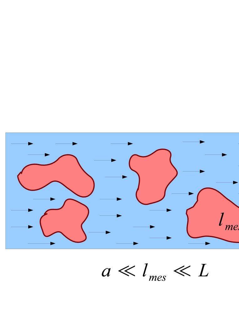
Figure 2: Scheme of the intermediate mixed state, with mesoscopic disordered regions inside the ordered matrix denoted by arrows.

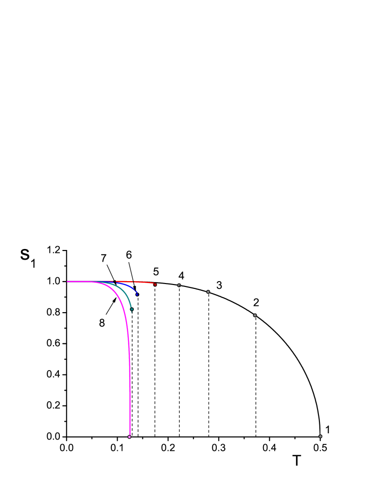
Figure 3: Imbalance order parameter as a function of temperature (in dimensionless units), with the marked points of the order-disorder phase transitions, for different disorder parameters: (1) $u=0$; (2) $u=0.1$; (3) $u=0.3$; (4) $u=0.4$; (5) $u=0.51$; (6) $u=0.75$; (7) $u=1$; (8) $u=1.5$.

Figure 4: Geometric weight of the ordered phase in the mixed system as a function of temperature (in dimensionless units), with the marked points of the order-disorder phase transitions, for the same disorder parameters as in Fig. 3.

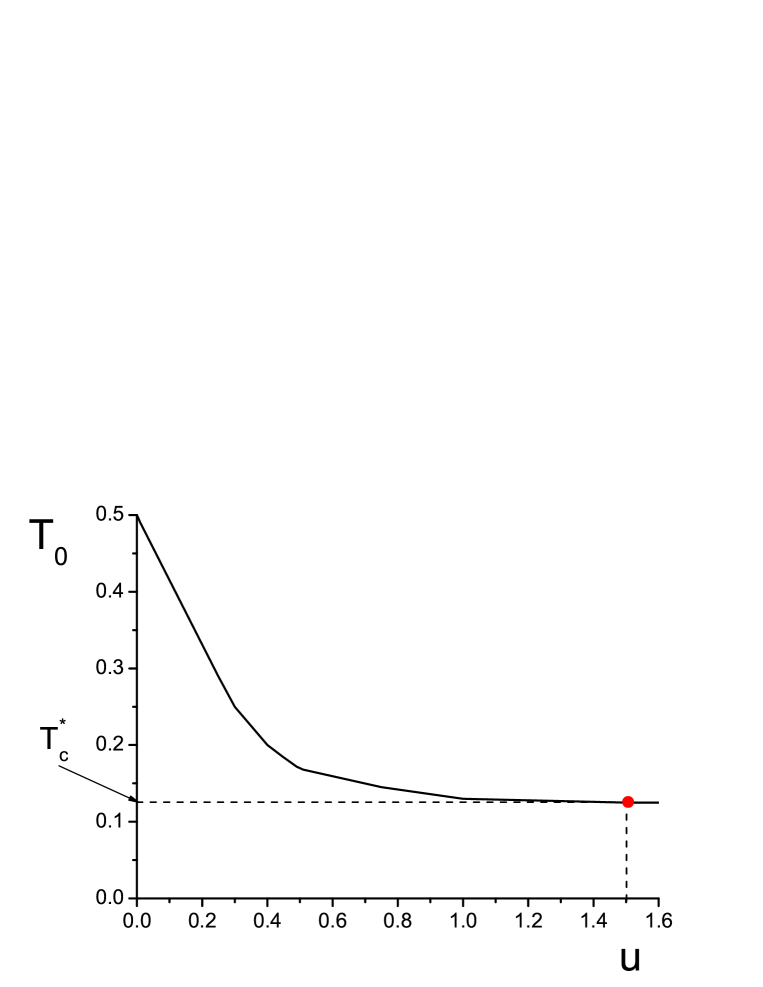
Figure 5: Order-disorder transition temperature (in dimensionless units) as a function of the disorder parameter $u$. The phase transition is of second order for $u=0$ and $u>3/2$; it is of first order for $0<u<3/2$; and $u=3/2$ corresponds to a tricritical point.

References

- [1] D. Jaksch and P. Zoller, Ann. Phys. (N.Y.) 315, 52 (2005).
- [2] O. Morsch and M. Oberthaler, Rev. Mod. Phys. 78, 179 (2006).
- [3] C. Moseley, O. Fialko, and K. Ziegler, Ann. Phys. (Berlin) 17, 561 (2008).
- [4] I. Bloch, J. Dalibard, and W. Zwerger, Rev. Mod. Phys. 80, 885 (2008).
- [5] V.I. Yukalov, Laser Phys. 19, 1 (2009).
- [6] R.A. Duine and H.T.C. Stoof, Phys. Rep. 396, 115 (2004).
- [7] V.A. Yurovsky, M. Olshanii, and D.S. Weiss, Adv. At. Mol. Opt. Phys. 55, 61 (2008).
- [8] J. Sebby-Strabley, M. Anderlini, P.S. Jessen, and J.V. Porto, Phys. Rev. A 73, 033605 (2006).
- [9] J. Sebby-Strabley, B.L. Brown, M. Anderlini, P.J. Lee, W.D. Phillips, J.V. Porto, and P.R. Johnson, Phys. Rev. Lett. 98, 200405 (2007).
- [10] P.J. Lee, M. Anderlini, B.L. Brown, J. Sebby-Strabley, W.D. Phillips, and J.V. Porto, Phys. Rev. Lett. 99, 020402 (2007).
- [11] S. Fölling, S. Trotzky, P. Cheinet, M. Feld, R. Saers, A. Widera, T. Müller, and I, Bloch, Nature 448, 1029 (2007).
- [12] P. Cheinet, S. Trotzky, M. Feld, U. Schnorrberger, M. Moreno-Cardoner, S. Fölling, and I. Bloch, Phys. Rev. Lett. 101, 090404 (2008).
- [13] I. Danshita, J.E. Williams, C.A.R. Sa de Melo, and C.W. Clark, Phys. Rev. A 76, 043606 (2007).
- [14] I. Danshita, C.A.R. Sa de Melo, and C.W. Clark, Phys. Rev. A 77, 063609 (2008).
- [15] V.I. Yukalov and E.P. Yukalova, Phys. Rev. A 78, 063610 (2008).
- [16] V.I. Yukalov and E.P. Yukalova, Laser Phys. Lett. 6, 235 (2009).
- [17] V.I. Yukalov and E.P. Yukalova, Phys. Lett. A 373, 1301 (2009).
- [18] V.O. Nesterenko, A.N. Novikov,, F.F. de Souza Cruz, and E.L. Lapolli, Laser Phys. 19, 616 (2009).
- [19] J.W. Gibbs, Collected Works, Vol. 1 (Longmans, New York, 1928).
- [20] J.W. Gibbs, Collected Works, Vol. 2 (Longmans, New York, 1931).
- [21] V.I. Yukalov, Theor. Math. Phys. 26, 274 (1976).
- [22] V.I. Yukalov, Theor. Math. Phys. 28, 652 (1976).
- [23] V.I. Yukalov, Phys. Lett. A 81, 249 (1981).
- [24] V.I. Yukalov, Phys. Lett. A 81, 433 (1981).
- [25] V.I. Yukalov, Phys. Lett. A 85, 68 (1981).
- [26] V.I. Yukalov, Physica A 108, 402 (1981).
- [27] V.I. Yukalov, Phys. Lett. A 125, 95 (1987).
- [28] V.I. Yukalov, Phys. Rep. 208, 395 (1991).
- [29] N. Bourbaki, Théorie des Ensembles (Hermann, Paris, 1958).
- [30] N.S. Krylov, Works on Foundations of Statistical Physics (Princeton University, Princeton, 1979).
- [31] N.N. Bogolubov, Problems of Dynamical Theory in Statistical Physics (North-Holland, Amsterdam, 1962).
- [32] N.N. Bogolubov, Dynamical Theory (Gordon and Breach, New York, 1990).
- [33] N.N. Bogolubov, Quantum and Classical Statistical Mechanics (Gordon and Breach, New York, 1991).
- [34] K.G. Wilson, Rev. Mod. Phys. 47, 773 (1975).
- [35] T.S. Cheng, D.D. Vvedensky, and J.F. Nicoll, Phys. Rep. 217, 279 (1992).
- [36] H. Baumgärtel and M. Wollenberg, Mathematical Scattering Theory (Birkhäuser, Basel, 1983).
- [37] S.P. Merkuriev and L. D. Faddeev, Quantum Scattering Theory for Several Particle Systems ( Kluwer, Dordrecht, 1993).
- [38] P.W. Courteille, V.S. Bagnato, and V.I. Yukalov, Laser Phys. 11, 659 (2001).
- [39] V.I. Yukalov, Laser Phys. Lett. 1, 435 (2004).
- [40] K. Bongs and K. Sengstock, Rep. Prog. Phys. 67, 907 (2004).
- [41] V.I. Yukalov and M.D. Girardeau, Laser Phys. Lett. 2, 375 (2005).
- [42] V.I. Yukalov, Laser Phys. Lett. 4, 632 (2007).
- [43] N.P. Proukakis and B. Jackson, J. Phys. B 41, 203002 (2008).
- [44] C.J. Pethik and H. Smith, Bose-Einstein Condensation in Dilute Gases (Cambridge University, Cambridge, 2008).
- [45] S. Kraft, F. Vogt, O. Appel, F. Riehle, and U. Sterr, Phys. Rev. Lett, 103, 130401 (2009).
- [46] S. Stellmer, M.K. Tey, B. Huang, R. Grimm, and F. Schreck, Phys. Rev. Lett. 103, 200401 (2009).
- [47] Y.N. Martinez de Escobar, P.G. Mickelson, M. Yan, G.J. DeSalvo, S.B. Nagel, and T.C. Killian, Phys. Rev. Lett. 103, 200402 (2009).
- [48] P.G. Mickelson, Y.N. Martinez de Escobar, M. Yan, B.J. DeSalvo, and T.C. Killian, Phys. Rev. A 81, 051601 (2010).
- [49] S. Giorgini, L.P. Pitaevskii, and S. Stringari, Rev. Mod. Phys. 80, 1215 (2008).
- [50] W. Ketterle and M.W. Zwierlein, Riv. Nuovo Cimento 31, 247 (2008).
- [51] F. Chevy and C. Mora, arXiv:1003.0801 (2010).
- [52] C. Chin, R. Grimm, P. Julienne, and E. Tiesinga, Rev. Mod. Phys. 82, 1225 (2010).
- [53] V. Yurovsky, arXiv:cond-mat/0611054 (2006).
- [54] A. Griesmaier, J. Phys. B 40, 91 (2007).
- [55] M.A. Baranov, Phys. Rep. 464, 71 (2008).
- [56] T.F. Gallagher, Rydberg Atoms (Cambridge University, Cambridge, 1994).
- [57] Ultracold Polar Molecules: Formation and Collisions, edited by J. Doyle, B. Friedrich, R.V. Krems, and F. Masnou-Seeuws [Eur. Phys. J. D 31, No. 2 (2004)].
- [58] V.I. Yukalov and E.P. Yukalova, J. Phys. A 29, 6429 (1996).
- [59] V.I. Yukalov, Int. J. Mod. Phys. B 3, 311 (1989).
- [60] V.I. Yukalov and A.S. Shumovsky, Lectures on Phase Transitions (World Scientific, Singapore, 1990).
- [61] V.I. Yukalov, Physica A 141, 352 (1987).
- [62] V.I. Yukalov, Physica A 144, 369 (1987).
- [63] M. Sangster and M. Dixon, Adv. Phys. 25, 247 (1976).
- [64] T. Köhler, T. Gasenzer, P.S. Julienne, and K. Burnett, Phys. Rev. Lett. 91, 230401 (2003).
- [65] H.G. Shuster, Deterministic Chaos (Physik, Weinheim, 1984).
- [66] Y.I. Neimark and P.S. Landa, Stochastic and Chaotic Oscillations (Kluwer, Dordrecht, 1992).
- [67] V.I. Yukalov, Laser Phys. Lett. 7, 467 (2010).
- [68] Y. Cheng and S.K. Adhikari, Laser Phys. Lett. 7, 824 (2010).
- [69] I.B. Mekhov and H. Ritsch, Laser Phys. 20, 694 (2010).
- [70] C. Weiss, Laser Phys. 20, 665 (2010).